Efficient Black-box Checking of Snapshot Isolation in Databases

Abstract.

Snapshot isolation (SI) is a prevalent weak isolation level that avoids the performance penalty imposed by serializability and simultaneously prevents various undesired data anomalies. Nevertheless, SI anomalies have recently been found in production cloud databases that claim to provide the SI guarantee. Given the complex and often unavailable internals of such databases, a black-box SI checker is highly desirable.

In this paper we present PolySI, a novel black-box checker that efficiently checks SI and provides understandable counterexamples upon detecting violations. PolySI builds on a novel characterization of SI using generalized polygraphs (GPs), for which we establish its soundness and completeness. PolySI employs an SMT solver and also accelerates SMT solving by utilizing the compact constraint encoding of GPs and domain-specific optimizations for pruning constraints. As demonstrated by our extensive assessment, PolySI successfully reproduces all of 2477 known SI anomalies, detects novel SI violations in three production cloud databases, identifies their causes, outperforms the state-of-the-art black-box checkers under a wide range of workloads, and can scale up to large-sized workloads.

PVLDB Reference Format:
PVLDB, 16(6): 1264 - 1276, 2023.
doi:10.14778/3583140.3583145

PVLDB Artifact Availability:
The source code, data, and/or other artifacts have been made available at %leave␣empty␣if␣no␣availability␣url␣should␣be␣sethttps://github.com/hengxin/PolySI-PVLDB2023-Artifacts.

1. Introduction

Database systems are an essential building block of many software systems and applications. Transactional access to databases simplifies concurrent programming by providing an abstraction for executing concurrent computations on shared data in isolation (Bernstein et al., 1986). The gold-standard isolation level, serializability (SER) (Papadimitriou, 1979), ensures that all transactions appear to execute serially, one after another. However, providing SER, especially in geo-replicated environments like modern cloud databases, is computationally expensive (Bailis et al., 2013; Lu et al., 2020).

Many databases provide weaker guarantees for transactions to balance the trade-off between data consistency and system performance. Snapshot isolation (SI) (Berenson et al., 1995) is one of the prevalent weaker isolation levels used in practice, which avoids the performance penalty imposed by SER and simultaneously prevents undesired data anomalies such as fractured reads, causality violations, and lost updates (Cerone and Gotsman, 2018). In addition to classic centralized databases such as Microsoft SQL Server (Server, 2022) and Oracle Database (Database, 2022), SI is supported by numerous production cloud database systems like Google’s Percolator (Peng and Dabek, 2010), MongoDB (MongoDB, 2022), TiDB (TiDB, 2022), YugabyteDB (YugabyteDB, 2022), Galera (Cluster, 2022), and Dgraph (Dgraph, 2022).

Unfortunately, as recently reported in (Kingsbury and Alvaro, 2020; testing of MongoDB 4.2.6, 2022; testing of TiDB 2.1.7, 2022), data anomalies have been found in several production cloud databases that claim to provide SI. This raises the question of whether such databases actually deliver the promised SI guarantee in practice. Given that their internals (e.g., source code) are often unavailable to the outsiders or hard to digest, a black-box SI checker is highly desirable.

A natural question then to ask is “What should an ideal black-box SI checker look like?” The SIEGE principle (Kingsbury and Alvaro, 2020) has already provided a strong baseline: an ideal checker would be sound (return no false positives), informative (report understandable counterexamples), effective (detect violations in real-world databases), general (compatible with different patterns of transactions), and efficient (add modest checking time even for workloads of high concurrency). Additionally, (i) we expect an ideal checker to be complete, thus missing no violations; and (ii) we also augment the generality criterion by requiring the checker to be compatible not only with general (read-only, write-only, and read-write) transaction workloads but also with standard key-value/SQL APIs. We call this extended principle SIEGE+.

None of the existing SI checkers, to the best of our knowledge, satisfies SIEGE+ (see Section 7 for the detailed comparison). For example, dbcop (Biswas and Enea, 2019) is incomplete, incurs exponentially increasing overhead under higher concurrency (Section 5.4), and returns no counterexamples upon finding a violation; Elle (Kingsbury and Alvaro, 2020) relies on specific database APIs such as lists and the (internal) timestamps of transactions to infer isolation anomalies, thus not conforming to our black-box setting.

The PolySI Checker. We present PolySI, a novel, black-box SI checker designed to achieve all the SIEGE+ criteria. PolySI builds on three key ideas in response to three major challenges.

First, despite previous attempts to characterize SI (Berenson et al., 1995; Adya, 1999; Xiong et al., 2020), its semantics is usually explained in terms of low-level implementation choices invisible to the database outsiders. Consequently, one must guess the dependencies (aka uncertain/unknown dependencies) between client-observable data, for example, which of the two writes was first recorded in the database.

We introduce a novel dependency graph, called generalized polygraph (GP), based on which we present a new sound and complete characterization of SI. There are two main advantages of a GP: (i) it naturally models the guesses by capturing all possible dependencies between transactions in a single compacted data structure; and (ii) it enables the acceleration of SMT solving by compacting constraints (see below) as demonstrated by our experiments.

Second, there have been recent advances in SAT and SMT solving for checking graph properties such as the MonoSAT solver (Bayless et al., 2015) and its successful application to the black-box checking of SER (Tan et al., 2020). The idea is to search for an acyclic graph where the nodes are transactions in the history and the edges meet certain constraints. We show that SMT techniques can also be applied to build an effective SI checker. This application is nontrivial as a brute-force approach would be inefficient due to the high computational complexity of checking SI (Biswas and Enea, 2019): the problem is NP-complete in general and $O(n^{c})$ with $c$ (resp. $n$) a fixed, yet in practice large, number of clients (resp. transactions), even for a single transaction history. In fact, checking SI is known to be asymptomatically more complex than checking SER (Biswas and Enea, 2019). In the context of SMT solving over graphs, SI leads to much larger search space due to its specific anomaly patterns (Cerone and Gotsman, 2018) while checking SER simply requires finding a cycle.

Thanks to our GP-based characterization of SI, we leverage its compact encoding of constraints on transaction dependencies to accelerate MonoSAT solving. Moreover, we develop domain-specific optimizations that further prune constraints, thereby reducing the search space. For example, PolySI prunes a constraint if an associated uncertain dependency would result in an SI violation with known dependencies.

Finally, although MonoSAT outputs cycles upon detecting a violation, they are still uninformative with respect to understanding how the violation actually occurred. Locating the actual causes of violations would facilitate debugging and repairing the defective implementations. For example, if an SI checker were to identify a lost update anomaly from the returned counterexample, developers could then focus on investigating the write-write conflict resolution mechanism. Hence, we design and integrate into PolySI a novel interpretation algorithm that explains the counterexamples returned by MonoSAT. More specifically, PolySI (i) recovers the violating scenario by bringing back any potentially involved transactions and dependencies eliminated during pruning and solving and (ii) finalizes the core participants to highlight the violation cause.

Main Contributions. In summary, we provide:

1. a new GP-based characterization of SI that both facilitates the modeling of uncertain transaction dependencies inherent to black-box testing and also enables the acceleration of constraint solving (Section 3);

2. a sound and complete GP-based checking algorithm for SI with domain-specific optimizations for pruning constraints (Section 4);

3. the PolySI tool comprising both our new checking algorithm and the interpretation algorithm for debugging; and

4. an extensive assessment of PolySI that demonstrates its fulfilment of SIEGE+ (Section 5). In particular, PolySI successfully reproduces all of 2477 known SI anomalies, detects novel SI violations in three production cloud databases, identifies their causes, outperforms the state-of-the-art black-box checkers under a wide range of workloads, and can scale up to large-sized workloads.

2. Preliminaries

2.1. Snapshot Isolation in a Nutshell

Snapshot isolation (SI) (Berenson et al., 1995) is one of the most prominent weaker isolation levels that modern (cloud) databases usually provide to avoid the performance penalty imposed by serializability (SER). Figure 1 shows a hierarchy of isolation levels where SI sits inbetween transactional causal consistency (Lloyd et al., 2013) and SER, and is not comparable to repeatable read (Adya, 1999).

Figure 1. A hierarchy of isolation levels. $A\rightarrow B$: $A$ is strictly weaker than $B$. CI: cut isolation (Bailis et al., 2013); RC: read committed (Berenson et al., 1995); RA: read atomicity (Bailis et al., 2016); RR: repeatable read (Adya, 1999); TCC: transactional causal consistency (Lloyd et al., 2013); SI: snapshot isolation (Cerone and Gotsman, 2018); SER: serializability (Berenson et al., 1995).

A transaction with SI always reads from a snapshot that reflects a single commit ordering of transactions and is allowed to commit if no concurrent transaction has updated the data that it intends to write. SI prevents various undesired data anomalies such as fractured reads, causality violations, lost updates, and long fork (Berenson et al., 1995; Cerone and Gotsman, 2018). The following examples illustrate two kinds of anomalies disallowed by SI. As we will see in Section 5, both anomalies have been detected by our PolySI checker in production cloud databases.

Example 1 (Causality Violation).

Alice posts a photo of her birthday party. Bob writes a comment to her post. Later, Carol sees Bob’s comment but not Alice’s post.

Example 2 (Lost Update).

Dan and Emma share a banking account with 10 dollars. Both simultaneously deposit 50 dollars. The resulting balance is 60, instead of 110, as one of the deposits is lost.

In this paper we focus on the prevalent strong session variant of SI (Daudjee and Salem, 2006; Cerone and Gotsman, 2018), which additionally requires a transaction to observe all the effects of the preceding transactions in the same session (Terry et al., 1994). Many production databases, including DGraph (Dgraph, 2022), Galera (Cluster, 2022), and CockroachDB (CockroachDB, 2022), provide this isolation level in practice.

2.2. Snapshot Isolation: Formal Definition

We recall the formalization of SI over dependency graphs, which serves as the theoretical foundation of PolySI. The following account is standard, see for example (Cerone and Gotsman, 2018), and Table 1 summarizes the notation used throughout the paper.

We consider a distributed key-value store managing a set of keys ${\sf Key}=\{\mathit{x},\mathit{y},\mathit{z},\dots\}$, which are associated with values from a set ${\sf Val}$. We denote by ${\sf Op}$ the set of possible read or write operations on keys: ${\sf Op}=\{{\sf R}_{\iota}(\mathit{x},\mathit{v}),{\sf W}_{\iota}(\mathit{x},\mathit{v})\mid\iota\in\mathsf{OpId},\mathit{x}\in{\sf Key},\mathit{v}\in{\sf Val}\}$, where $\mathsf{OpId}$ is the set of operation identifiers. We omit operation identifiers when they are unimportant.

Table 1. Notation

Category	Notation	Meaning
KV Store	${\sf Key}$	set of keys
	${\sf Val}$	set of values
	${\sf Op}$	set of operations
Relations	$R?$	reflexive closure of $R$
	$R^{+}$	transitive closure of $R$
	$R\;;\;S$	composition of $R$ with $S$
Dependency	SO, WR, WW, RW	dependency relations/edges
Graph	$G=(V,E,C)$	(generalized) polygraph
	$V_{G}$, $E_{G}$, $C_{G}$	components of $G$
	$G|_{F}$	digraph with set $F$ of edges
Algorithm	$\mathcal{H}=(\mathcal{T},\textsf{SO})$	history to check
	$\mathit{I}$	SI induced graph
	$\mathsf{BV}$	set of Boolean variables
	$\mathsf{CL}$	set of clauses

2.2.1. Relations, Orderings, Graphs, and Logics

A binary relation $R$ over a given set $A$ is a subset of $A\times A$, i.e., $R\subseteq A\times A$. For $a,b\in A$, we use $(a,b)\in R$ and $a\xrightarrow{R}b$ interchangeably. We use $R{?}$ and $R^{+}$ to denote the reflexive closure and the transitive closure of $R$, respectively. A relation $R\subseteq A\times A$ is acyclic if $R^{+}\cap I_{A}=\emptyset$, where $I_{A}\triangleq\{(a,a)\mid a\in A\}$ is the identity relation on $A$. Given two binary relations $R$ and $S$ over set $A$, we define their composition as $R\;;\;S=\{(a,c)\mid\exists b\in A:a\xrightarrow{R}b\xrightarrow{S}c\}$. A strict partial order is an irreflexive and transitive relation. A strict total order is a relation that is a strict partial order and total.

For a directed labeled graph $G=(V,E)$, we use $V_{G}$ and $E_{G}$ to denote the set of vertices and edges in $G$, respectively. For a set $F$ of edges, $G|_{F}$ denotes the directed labeled graph that has the set $V$ of vertices and the set $F$ of edges.

In logical formulas, we write $\_$ for irrelevant parts that are implicitly existentially quantified. We use $\exists!$ to mean “unique existence.”

2.2.2. Transactions and Histories

Definition 3.

A transaction is a pair $(\mathit{O},{\sf po})$, where $\mathit{O}\subseteq{\sf Op}$ is a finite, non-empty set of operations and ${\sf po}\subseteq\mathit{O}\times\mathit{O}$ is a strict total order called the program order.

For a transaction $T$, we let $T\vdash{\sf W}(\mathit{x},\mathit{v})$ if $T$ writes to $\mathit{x}$ and the last value written is $\mathit{v}$, and $T\vdash{\sf R}(\mathit{x},\mathit{v})$ if $T$ reads from $\mathit{x}$ before writing to it and $\mathit{v}$ is the value returned by the first such read. We also use ${\sf WriteTx}_{\mathit{x}}=\{T\mid T\vdash{\sf W}(\mathit{x},\_)\}$.

Clients interact with the store by issuing transactions during sessions. We use a history to record the client-visible results of such interactions. For conciseness, we consider only committed transactions in the formalism (Cerone and Gotsman, 2018); see further discussions in Section 4.5.

Definition 4.

A history is a pair $\mathcal{H}=(\mathcal{T},\textsf{SO})$, where $\mathcal{T}$ is a set of transactions with disjoint sets of operations and the session order $\textsf{SO}\subseteq\mathcal{T}\times\mathcal{T}$ is the union of strict total orders on disjoint sets of $\mathcal{T}$, which correspond to transactions in different sessions.

2.2.3. Dependency Graph-based Characterization of SI

A dependency graph extends a history with three relations (or typed edges, in terms of graphs): WR, WW, and RW, representing three possibility of dependencies between transactions in this history (Cerone and Gotsman, 2018). The WR relation associates a transaction that reads some value with the one that writes this value. The WW relation stipulates a strict total order (aka the version order (Adya, 1999)) among the transactions on the same key. The RW relation is derived from WR and WW, relating a transaction that reads some value to the one that overwrites this value, in terms of the version orders specified by the WW relation.

Definition 5.

A dependency graph is a tuple $\mathcal{G}=(\mathcal{T},\textsf{SO},\textsf{WR},\\ \textsf{WW},\textsf{RW})$, where $(\mathcal{T},\textsf{SO})$ is a history and

1. $\textsf{WR}:{\sf Key}\to 2^{\mathcal{T}\times\mathcal{T}}$ is such that

   • $\forall\mathit{x}\in{\sf Key}.\;\forall S\in\mathcal{T}.\;S\vdash{\sf R}(\mathit{x},\_)\!\!\implies\!\!\exists!T\in\mathcal{T}.\;T\xrightarrow{\textsf{WR}(\mathit{x})}S$

   • $\forall\mathit{x}\in{\sf Key}.\;\forall T,S\in\mathcal{T}.\;T\xrightarrow{\textsf{WR}(x)}S\implies T\neq S\land\exists\mathit{v}\in{\sf Val}.\;T\vdash{\sf W}(\mathit{x},\mathit{v})\land S\vdash{\sf R}(\mathit{x},\mathit{v})$.

2. $\textsf{WW}:{\sf Key}\to 2^{\mathcal{T}\times\mathcal{T}}$ is such that for every $\mathit{x}\in{\sf Key}$, $\textsf{WW}(\mathit{x})$ is a strict total order on the set ${\sf WriteTx}_{\mathit{x}}$;

3. $\textsf{RW}:{\sf Key}\to 2^{\mathcal{T}\times\mathcal{T}}$ is such that $\forall T,S\in\mathcal{T}.\;\forall\mathit{x}\in{\sf Key}.\;T\xrightarrow{\textsf{RW}(\mathit{x})}S\iff T\neq S\land\exists T^{\prime}\in\mathcal{T}.\;T^{\prime}\xrightarrow{\textsf{WR}(\mathit{x})}T\land T^{\prime}\xrightarrow{\textsf{WW}(\mathit{x})}S$.

We denote a component of $\mathcal{G}$, such as WW, by $\textsf{WW}_{\mathcal{G}}$. We write $T\xrightarrow{\textsf{WR}/\textsf{WW}/\textsf{RW}}S$ when the key $\mathit{x}$ in $T\xrightarrow{\textsf{WR}(\mathit{x})/\textsf{WW}(\mathit{x})/\textsf{RW}(\mathit{x})}S$ is irrelevant or the context is clear.

Intuitively, a history satisfies SI if and only if it can be extended to a dependency graph that contains only cycles (if any) with at least two adjacent RW edges. Formally,

Theorem 6 (Dependency Graph-based Characterization of SI (Theorem 4.1 of (Cerone and Gotsman, 2018))).

For a history $\mathcal{H}=(\mathcal{T},\textsf{SO})$,

$$\mathcal{H}\models\textsc{SI} \iff\mathcal{H}\models\textsc{Int}\;\land$$

$$\exists\textsf{WR},\textsf{WW},\textsf{RW}.\;\mathcal{G}=(\mathcal{H},\textsf{WR},\textsf{WW},\textsf{RW})\;\land$$

$$\quad(((\textsf{SO}_{\mathcal{G}}\cup\textsf{WR}_{\mathcal{G}}\cup\textsf{WW}_{\mathcal{G}})\;;\;\textsf{RW}_{\mathcal{G}}?)\text{\it\; is acyclic}).$$

The internal consistency axiom Int ensures that, within a transaction, a read from a key returns the same value as the last write to or read from this key in the transaction.

2.3. The SI Checking Problem

Definition 7.

The SI checking problem is the decision problem of determining whether a given history $\mathcal{H}$ satisfies SI, i.e., is $\mathcal{H}\models\textsc{SI}$?

We take the common “UniqueValue” assumption on histories (Adya, 1999; Biswas and Enea, 2019; Crooks et al., 2017; Bouajjani et al., 2017; Tan et al., 2020): for each key, every write to the key assigns a unique value. For database testing, we can produce such histories by ensuring the uniqueness of the values written on the client side (or workload generator) using, e.g., the client identifier and local counter. Under this assumption, each read can be associated with the transaction that issues the corresponding write (Cerone and Gotsman, 2018).

Theorem 6 provides a brute-force approach to the SI checking problem: enumerate all possible WW relations and check whether any of them results in a dependency graph that contains only cycles with at least two adjacent RW edges. This approach is, however, prohibitively expensive.

2.4. Polygraphs

A dependency graph extending a history represents one possibility of dependencies between transactions in this history. To capture all possible dependencies between transactions in a single structure, we rely on polygraphs (Papadimitriou, 1979). Intuitively, a polygraph can be viewed as a family of dependency graphs.

(a) A polygraph

(b) A generalized polygraph

Figure 2. Examples of polygraphs and generalized polygraphs. WR, WW, and RW relations are represented by solid, dashed, and dotted arrows, respectively.

Definition 8.

A polygraph $G=(V,E,C)$ associated with a history $\mathcal{H}=(\mathcal{T},\textsf{SO})$ is a directed labeled graph $(V,E)$ called the known graph, together with a set $C$ of constraints such that

• $V$ corresponds to all transactions in the history $\mathcal{H}$;

• $E=\{(T,S,\textsf{SO})\mid T\xrightarrow{\textsf{SO}}S\}\cup\{(T,S,\textsf{WR})\mid T\xrightarrow{\textsf{WR}}S\}$, where SO and WR, when used as the third component of an edge, are edge labels (i.e., types); and

• $C=\{\langle(T_{k},T_{i},\textsf{WW}),(T_{j},T_{k},\textsf{RW})\rangle\mid(T_{i}\xrightarrow{\textsf{WR}(\mathit{x})}T_{j})\land T_{k}\in{\sf WriteTx}_{\mathit{x}}\land T_{k}\neq T_{i}\land T_{k}\neq T_{j}\}$.

As shown in Figure 2(a), for a pair of transactions $T_{i}$ and $T_{j}$ such that $T_{i}\xrightarrow{\textsf{WR}(\mathit{x})}T_{j}$ and a transaction $T_{k}$ that writes $\mathit{x}$, the constraint $\langle(T_{k},T_{i},\textsf{WW}),(T_{j},T_{k},\textsf{RW})\rangle$ captures the unknown dependencies that “either $T_{k}$ happened before $T_{i}$ or $T_{k}$ happened after $T_{j}$.”

3. Characterizing SI using Generalized Polygraphs

In this section we introduce generalized polygraphs with generalized constraints and use them to characterize SI. By compacting several constraints together, using generalized constraints leads to a compact encoding which in turn helps accelerate the solving process (see Section 5.4.3).

3.1. Generalized Polygraphs

In a polygraph, a constraint involves only a single pair of transactions related by WR, like $T_{i}$ and $T_{j}$ on $\mathit{x}$ in Figure 2(a). Thus, several constraints are needed when there are multiple transactions reading the value of $\mathit{x}$ from $T_{i}$. To compact these constraints, we introduce generalized polygraphs with generalized constraints.

Definition 1.

A generalized polygraph $G=(V,E,C)$ associated with a history $\mathcal{H}=(\mathcal{T},\textsf{SO})$ is a directed labeled graph $(V,E)$ called the known graph, together with a set $C$ of generalized constraints such that

• $V$ corresponds to all transactions in the history $\mathcal{H}$;

• $E\subseteq V\times V\times\mathcal{L}$ is a set of edges with labels (i.e., types) from $\mathcal{L}=\{\textsf{SO},\textsf{WR},\textsf{WW},\textsf{RW}\}$; and

• $C=\big{\{}\big{\langle}\mathit{either}\triangleq\{(T,S,\textsf{WW})\}\;\cup\bigcup\limits_{T^{\prime}\in\textsf{WR}(\mathit{x})(T)}\!\!\{(T^{\prime},S,\textsf{RW})\},\\ \mathit{or}\triangleq\{(S,T,\textsf{WW})\}\;\cup\bigcup\limits_{S^{\prime}\in\textsf{WR}(\mathit{x})(S)}\!\!\{(S^{\prime},T,\textsf{RW})\}\big{\rangle}\mid T\in{\sf WriteTx}_{\mathit{x}}\land S\in{\sf WriteTx}_{\mathit{x}}\land T\neq S\big{\}}$.

A generalized constraint is a pair of sets of edges of the form $\langle\mathit{either},\mathit{or}\rangle$. The $\mathit{either}$ part handles the possibility of $T$ being ordered before $S$ via a WW edge. This forces each transaction $T^{\prime}$ that reads the value of $\mathit{x}$ from $T$ to be ordered before $S$ via an RW edge. Symmetrically, the $\mathit{or}$ part handles the possibility of $S$ being ordered before $T$ via a WW edge. This forces each transaction $S^{\prime}$ that reads the value of $\mathit{x}$ from $S$ to be ordered before $T$ via an RW edge.

Example 2 (Generalized Polygraphs vs. Polygraphs).

In Figure 2(b), both transactions $T$ and $S$ write to $\mathit{x}$, and $T^{\prime}$ and $S^{\prime}$ read the values of $\mathit{x}$ from $T$ and $S$, respectively. The possible dependencies between these transactions can be compactly expressed as a single generalized constraint $\langle\{(T,S,\textsf{WW}),(T^{\prime},S,\textsf{RW})\},\{(S,T,\textsf{WW}),(S^{\prime},T,\textsf{RW})\}\rangle$, which corresponds to two constraints: $\langle(T,S,\textsf{WW}),(S^{\prime},T,\textsf{RW})\rangle$ and $\langle(S,T,\textsf{WW}),(T^{\prime},S,\textsf{RW})\rangle$.

Note that a generalized polygraph may contain edges of any type in $E$ such that a “pruned” generalized polygraph (Section 4.3) is still a generalized polygraph. For a generalized polygraph $G=(V,E,C)$ and a label $L\in\mathcal{L}$, we use $V_{G}$, $E_{G}$, $C_{G}$, and $L_{G}$ to denote the set $V$ of vertices, the set $E$ of known edges, the set $C$ of constraints, and the set of known edges with label $L$ in $E$, respectively. For a generalized polygraph $G=(V,E,C)$ and a set $F$ of edges, we use $G|_{F}$ to denote the directed labeled graph that has the set $V$ of vertices and the set $F$ of edges. For any two subsets $R,S\subseteq E$, we define their composition as $R\;;\;S=\{(a,c,L_{1}\;;\;L_{2})\mid\exists b\in V:(a,b,L_{1})\in R\land(b,c,L_{2})\in S\}$, where $L_{1}\;;\;L_{2}$ is a newly introduced label used when composing edges. In the sequel, we use generalized polygraphs, but sometimes we still refer to them as polygraphs.

3.2. Characterizing SI

According to Theorem 6, we are interested in the induced graph of a generalized polygraph $\mathit{G}$, obtained by composing the edges of $\mathit{G}$ according to the rule $((\textsf{SO}\cup\textsf{WR}\cup\textsf{WW})\;;\;\textsf{RW}?)$.

Definition 3.

The induced SI graph of a polygraph $\mathit{G}=(V,E,C)$ is the graph $G^{\prime}=(V,E,C,\mathcal{R})$, where $\mathcal{R}=(\textsf{SO}\cup\textsf{WR}\cup\textsf{WW})\;;\;\textsf{RW}?$ is the induce rule.

The concept of compatible graphs gives a meaning to polygraphs and their induced SI graphs. A graph is compatible with a polygraph when it is a resolution of the constraints of the polygraph. Thus, a polygraph corresponds to a family of its compatible graphs.

Definition 4.

A directed labeled graph $G^{\prime}=(V^{\prime},E^{\prime})$ is compatible with a generalized polygraph $G=(V,E,C)$ if

• $V^{\prime}=V$;

• $E^{\prime}\supseteq E$; and

• $\forall\langle\mathit{either},\mathit{or}\rangle\in C.\;(\mathit{either}\subseteq E^{\prime}\land\mathit{or}\cap E^{\prime}=\emptyset)\lor(\mathit{or}\subseteq E^{\prime}\land\mathit{either}\cap E^{\prime}=\emptyset)$.

By applying the induce rule $\mathcal{R}$ to a compatible graph of a polygraph, we obtain a compatible graph with the induced SI graph of this polygraph.

Definition 5.

Let $G^{\prime}=(V^{\prime},E^{\prime})$ be a compatible graph with a polygraph $G$. Then $G^{\prime}|_{(\textsf{SO}_{G^{\prime}}\;\cup\;\textsf{WR}_{G^{\prime}}\;\cup\;\textsf{WW}_{G^{\prime}})\;;\;\textsf{RW}_{G^{\prime}}?}$ is a compatible graph with the induced SI graph of $G$.

Example 6 (Compatible Graphs).

There are two compatible graphs with the generalized polygraph of Figure 2(b): one is with the edge set $\{(T,T^{\prime},\textsf{WR}),(S,S^{\prime},\textsf{WR}),(T,S,\textsf{WW}),(T^{\prime},S,\textsf{RW})\}$, and the other is with $\{(T,T^{\prime},\textsf{WR}),(S,S^{\prime},\textsf{WR}),(S,T,\textsf{WW}),(S^{\prime},T,\textsf{RW})\}$.

Accordingly, there are also two compatible graphs with the induced SI graph of the polygraph of Figure 2(b): one is with the edge set $\{(T,T^{\prime},\textsf{WR}),(S,S^{\prime},\textsf{WR}),(T,S,\textsf{WW}),(T,S,\textsf{WR}\;;\;\textsf{RW})\}$. The edge $(T,S,\textsf{WR}\;;\;\textsf{RW})$ is obtained from $(T,T^{\prime},\textsf{WR})\;;\;(T^{\prime},S,\textsf{RW})$. It is identical to $(T,S,\textsf{WW})$ if the edge types are ignored. The other is with $\{(T,T^{\prime},\textsf{WR}),(S,S^{\prime},\textsf{WR}),(S,T,\textsf{WW}),(S,T,\textsf{WR}\;;\;\textsf{RW})\}$. Similarly, $(S,T,\textsf{WR}\;;\;\textsf{RW})$ is identical to $(S,T,\textsf{WW})$ if the edge types are ignored.

We are concerned with the acyclicity of polygraphs and their induced SI graphs.

Definition 7.

An induced SI graph is acyclic if there exists an acyclic compatible graph with it, when the edge types are ignored. A polygraph is SI-acyclic if its induced SI graph is acyclic.

Finally, we present the generalized polygraph-based characterization of SI. Its proof can be found in Appendix B. The key lies in the correspondence between compatible graphs of polygraphs and dependency graphs.

Theorem 8 (Generalized Polygraph-based Characterization of SI).

A history $\mathcal{H}$ satisfies SI if and only if $\mathcal{H}\models\textsc{Int}$ and the generalized polygraph of $\mathcal{H}$ is SI-acyclic.

4. The Checking Algorithm for SI

Given a history $\mathcal{H}$, PolySI encodes the induced SI graph of the generalized polygraph of $\mathcal{H}$ into an SAT formula and utilizes the MonoSAT solver (Bayless et al., 2015) to test its acyclicity. We choose MonoSAT mainly because, compared to conventional SMT solvers such as Z3, it is more efficient in checking graph properties (Bayless et al., 2015).

The main challenge is that the size (measured as the number of variables and clauses) of the resulting SAT formula may be too large for MonoSAT to solve in reasonable time. Hence, PolySI prunes constraints of the generalized polygraph of $\mathcal{H}$ before encoding. As we will see in Section 5.4, this pruning process is crucial to PolySI’s high performance. Additionally, solving is accelerated by utilizing, instead of original polygraphs, generalized polygraphs with compact generalized constraints.

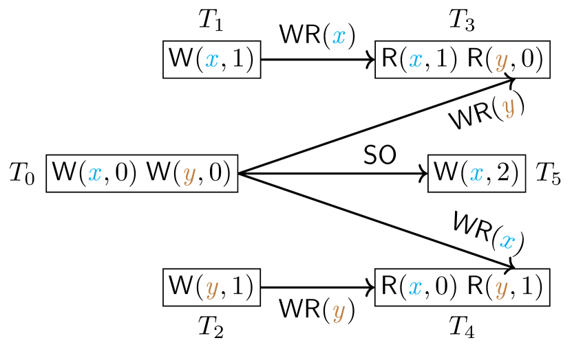
(a) A “long fork” history with SO and WR edges. $T_{0}$ and $T_{5}$ are on the same session.

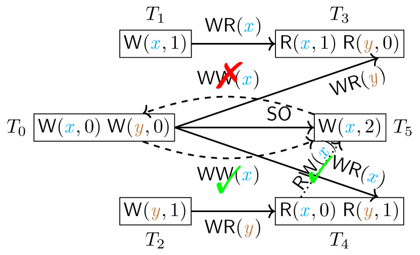
(b) The $T_{5}\xrightarrow{\textsf{WW}(\mathit{x})}T_{0}$ case is pruned due to the cycle $T_{0}\xrightarrow{\textsf{SO}}T_{5}\xrightarrow{\textsf{WR}(\mathit{x})}T_{0}$.

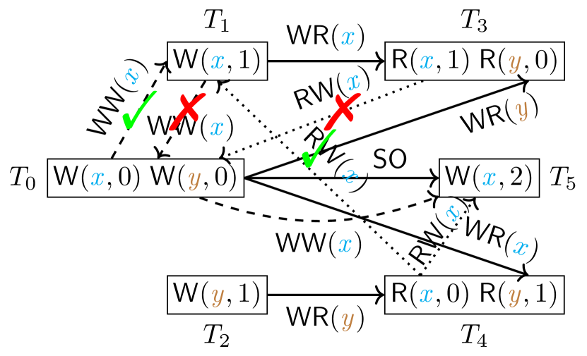
(c) The $T_{1}\xrightarrow{\textsf{WW}(\mathit{x})}T_{0}$ case is pruned due to the cycle $T_{3}\xrightarrow{\textsf{RW}(\mathit{x})}T_{0}\xrightarrow{\textsf{WR}(\mathit{y})}T_{3}$.

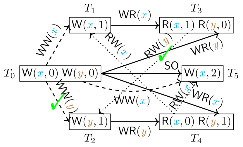
(d) The $T_{2}\xrightarrow{\textsf{WW}(\mathit{y})}T_{0}$ case is pruned and the $T_{0}\xrightarrow{\textsf{WW}(\mathit{y})}T_{2}$ case become known.

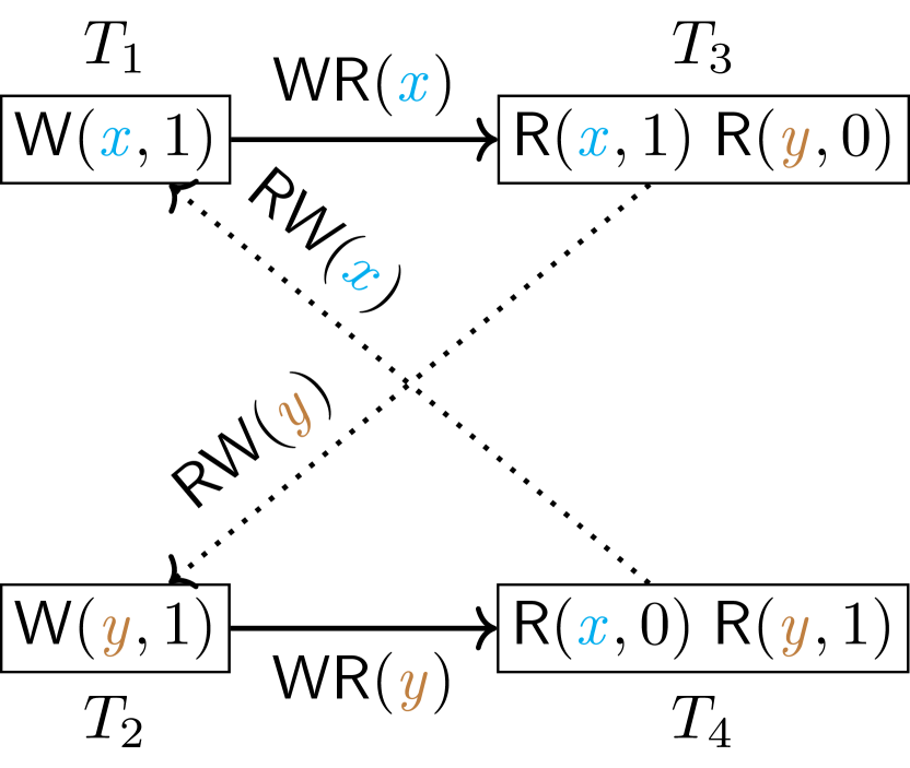
(e) The undesired and violating cycle found by MonoSAT.

Figure 3. The “long fork” anomaly: an illustrating example of PolySI.

4.1. Overview

The procedure CheckSI (line 1 of Algorithm 1) outlines the checking algorithm. First, if $\mathcal{H}$ does not satisfy the Int axiom, the checking algorithm terminates and returns false (line 2; see Section 4.5 for the predicates AbortedReads and IntermediateReads). The algorithm proceeds otherwise in the following three steps:

• construct the generalized polygraph $\mathit{G}$ of $\mathcal{H}$ (lines 4 and 5);

• prune constraints in the polygraph $\mathit{G}$ (line 6); and

• encode the induced SI graph, denoted $\mathit{I}$, of $\mathit{G}$ after pruning into an SAT formula (line 8), and call MonoSAT to test whether $\mathit{I}$ is acyclic (line 9).

Algorithm 1 depicts the core procedures of pruning and encoding. The remaining procedures are given in Appendix A.

Before diving into details, we illustrate our algorithm using the example history in Figure 3(a), which exemplifies the well-known “long fork” anomaly in SI (Sovran et al., 2011; Cerone and Gotsman, 2018). Specifically, transaction $T_{0}$ writes to both keys $\mathit{x}$ and $\mathit{y}$. Transactions $T_{1}$ and $T_{2}$ concurrently write to $\mathit{x}$ and $\mathit{y}$, respectively. Transaction $T_{3}$ sees the write by $T_{1}$, but not the write by $T_{2}$, while $T_{4}$ sees the write by $T_{2}$, but not the write by $T_{1}$. The session committing $T_{0}$ then issues $T_{5}$ to update $\mathit{x}$.

Pruning Constraints. To check whether this history satisfies SI, we must determine the order between $T_{0}$, $T_{1}$, and $T_{5}$ (on $\mathit{x}$) and the order between $T_{0}$ and $T_{2}$ (on $\mathit{y}$). Consider first the constraint on the order between $T_{0}$ and $T_{5}$ shown in Figure 3(b). Due to $T_{0}\xrightarrow{\textsf{SO}}T_{5}$, the $T_{5}\xrightarrow{\textsf{WW}(\mathit{x})}T_{0}$ case would introduce an undesired cycle. Therefore, this case can be safely pruned and the other case of $T_{0}\xrightarrow{\textsf{WW}(\mathit{x})}T_{5}$, along with the edge $T_{4}\xrightarrow{\textsf{RW}(\mathit{x})}T_{5}$, become known.

Figure 3(c) shows the constraint on the order between $T_{0}$ and $T_{1}$: $\langle\mathit{either}=\{(T_{1},T_{0},\textsf{WW}),(T_{3},T_{0},\textsf{RW}\},\mathit{or}=\{(T_{0},T_{1},\textsf{WW}),(T_{4},T_{1},\textsf{RW})\}\rangle$. Consider first the $\mathit{either}$ case. Note that the edge $T_{3}\xrightarrow{\textsf{RW}(\mathit{x})}T_{0}$ is in an undesired cycle $T_{3}\xrightarrow{\textsf{RW}(\mathit{x})}T_{0}\xrightarrow{\textsf{WR}(\mathit{y})}T_{3}$, which contains only a single RW edges. Hence, the $\mathit{either}$ case could be safely pruned, without SAT encoding and solving. Conversely, the $\mathit{or}$ case does not introduce undesired cycles. Thus, the edges in the $\mathit{or}$ case become known, before SAT encoding and solving.

Similarly, the $\mathit{either}$ case of the constraint on the order between $T_{0}$ and $T_{2}$, namely $\langle\mathit{either}=\{(T_{2},T_{0},\textsf{WW}),(T_{4},T_{0},\textsf{RW}\},\mathit{or}=\\ \{(T_{0},T_{2},\textsf{WW}),(T_{4},T_{2},\textsf{RW})\}\rangle$, could be safely pruned (not shown in Figure 3(d)), and the edges in the $\mathit{or}$ case become known.

SAT Encoding. The order between $T_{1}$ and $T_{5}$ is still uncertain after pruning in Figure 3(d). We encode the constraint $\langle\mathit{either}=\{(T_{1},T_{5},\textsf{WW}),(T_{3},T_{5},\textsf{RW})\},\mathit{or}=\{(T_{5},T_{1},\textsf{WW})\}\rangle$ on the order as a SAT formula

$$(\mathsf{BV}_{1,5}\land\mathsf{BV}_{3,5}\land\lnot\mathsf{BV}_{5,1})\lor(\mathsf{BV}_{5,1}\land\lnot\mathsf{BV}_{1,5}\land\lnot\mathsf{BV}_{3,5}),$$

where $\mathsf{BV}_{i,j}$ is a Boolean variable indicating the existence of the edge from $T_{i}$ to $T_{j}$ in the pruned polygraph. We then encode the induced SI graph, denoted $\mathit{I}$. Since $T_{2}\xrightarrow{\textsf{WR}(\mathit{y})}T_{4}\xrightarrow{\textsf{RW}(\mathit{x})}T_{5}$, we have $\mathsf{BV}^{\mathit{I}}_{2,5}=\mathsf{BV}_{2,4}\land\mathsf{BV}_{4,5}$, where $\mathsf{BV}^{\mathit{I}}_{i,j}$ is a Boolean variable indicating the existence of the edge from $T_{i}$ to $T_{j}$ in $\mathit{I}$. Similarly, we have $\mathsf{BV}^{\mathit{I}}_{1,2}=\mathsf{BV}_{1,3}\land\mathsf{BV}_{3,2}$ and $\mathsf{BV}^{\mathit{I}}_{2,1}=\mathsf{BV}_{2,4}\land\mathsf{BV}_{4,1}$. In contrast, since it is possible that $T_{3}\xrightarrow{\textsf{RW}(\mathit{x})}T_{5}$, we have $\mathsf{BV}^{\mathit{I}}_{1,5}=\mathsf{BV}_{1,3}\land\mathsf{BV}_{3,5}$.

MonoSAT Solving. Finally, we feed the SAT formula to MonoSAT for an acyclicity test of the graph $\mathit{I}$. MonoSAT successfully finds an undesired cycle $T_{1}\xrightarrow{\textsf{WR}(\mathit{x})}T_{3}\xrightarrow{\textsf{RW}(\mathit{y})}T_{2}\xrightarrow{\textsf{WR}(\mathit{y})}T_{4}\xrightarrow{\textsf{RW}(\mathit{x})}T_{1}$, which contains two non-adjacent RW edges; see Figure 3(e). Therefore, this history violates SI.

Algorithm 1 The PolySI algorithm for checking SI

1:procedure CheckSI($\mathcal{H}$)

2:    if $\mathcal{H}\not\models\textsc{Int}\lor\textsc{AbortedReads}\lor\textsc{IntermediateReads}$ 

3:        return false    

4:    CreateKnownGraph($\mathcal{H}$) $\triangleright$ see Appendix A

5:    GenerateConstraints($\mathcal{H}$) $\triangleright$ see Appendix A

6:    if $\lnot\textsc{{PruneConstraints}}(\hbox{})$ 

7:        return false     

8:    SAT-Encode()

9:    return MonoSAT-Solve() $\triangleright$ see Appendix A

10:

11:procedure PruneConstraints()

12:    repeat

13:        $\mathit{Dep}\leftarrow\mathit{G}|_{\textsf{SO}_{\mathit{G}}\cup\textsf{WR}_{\mathit{G}}\cup\textsf{WW}_{\mathit{G}}}$

14:        $\mathit{AntiDep}\leftarrow\mathit{G}|_{\textsf{RW}_{\mathit{G}}}$

15:        $\mathit{KI}\leftarrow\mathit{Dep}\cup(\mathit{Dep}\;;\;\mathit{AntiDep})$

16:        $\mathit{reachability}\leftarrow\textsc{{Reachability}}(\mathit{KI})$ $\triangleright$ using Floyd-Warshall algorithm (Cormen et al., 2009).

17:        for all $\mathit{cons}\leftarrow\langle\mathit{either},\mathit{or}\rangle\in\mathit{C}_{\mathit{G}}$ 

18:           for all $(\mathit{from},\mathit{to},\mathit{type})\in\mathit{either}$  $\triangleright$ for the “$\mathit{either}$” possibility

19:               if $\mathit{type}=\textsf{WW}$ 

20:                  if $(\mathit{to},\mathit{from})\in\mathit{reachability}$ 

21:                      $\mathit{C}_{\mathit{G}}\leftarrow\mathit{C}_{\mathit{G}}\setminus\{\mathit{cons}\}$

22:                      $\mathit{E}_{\mathit{G}}\leftarrow\mathit{E}_{\mathit{G}}\cup\mathit{or}$

23:                      break the “for all $(\mathit{from},\mathit{to},\mathit{type})\in\mathit{either}$” loop                   

24:               else$\triangleright$ $\mathit{type}=\textsf{RW}$

25:                  for all $\mathit{prec}\in\mathit{V}_{\mathit{Dep}}$ such that $(\mathit{prec},\mathit{from},\_)\in\mathit{E}_{\mathit{Dep}}$ 

26:                      if $(\mathit{to},\mathit{prec})\in\mathit{reachability}$ 

27:                          $\mathit{C}_{\mathit{G}}\leftarrow\mathit{C}_{\mathit{G}}\setminus\{\mathit{cons}\}$

28:                          $\mathit{E}_{\mathit{G}}\leftarrow\mathit{E}_{\mathit{G}}\cup\mathit{or}$

29:                          break the “for all $(\mathit{from},\mathit{to},\mathit{type})\in\mathit{either}$” loop                                                                   

30:           for all $(\mathit{from},\mathit{to},\mathit{type})\in\mathit{or}$  $\triangleright$ for the “$\mathit{or}$” possibility

31:               the same with the “$\mathit{either}$” possibility except that it returns False

32:                if both $\mathit{either}$ and $\mathit{or}$ possibilities of a constraint are pruned                    

33:    until $\mathit{C}_{\mathit{G}}$ remains unchanged

34:    return True

35:

36:procedure SAT-Encode()

37:    for all $\mathit{v}_{i},\mathit{v}_{j}\in\mathit{V}_{\mathit{G}}$ such that $i\neq j$ 

38:        $\mathsf{BV}\leftarrow\mathsf{BV}\cup\{\mathsf{BV}_{i,j},\mathsf{BV}^{\mathit{I}}_{i,j}\}$     

39:    for all $(\mathit{v}_{i},\mathit{v}_{j})\in\mathit{E}_{\mathit{G}}$  $\triangleright$ encode the known graph of $\mathit{G}$

40:        $\mathsf{CL}\leftarrow\mathsf{CL}\cup\{\mathsf{BV}_{i,j}=\textsf{True}\}$     

41:    for all $\langle\mathit{either},\mathit{or}\rangle\in\mathit{C}_{\mathit{G}}$  $\triangleright$ encode the constraints of $\mathit{G}$

42:        $\mathsf{CL}\leftarrow\mathsf{CL}\;\cup\;\Big{\{}\bigl{(}\bigwedge\limits_{(\mathit{v}_{i},\mathit{v}_{j},\_)\in\mathit{either}}\!\!\!\!\mathsf{BV}_{i,j}\land\bigwedge\limits_{(\mathit{v}_{i},\mathit{v}_{j},\_)\in\mathit{or}}\!\!\!\!\lnot\mathsf{BV}_{i,j}\bigr{)}\;\lor\;\bigl{(}\bigwedge\limits_{(\mathit{v}_{i},\mathit{v}_{j},\_)\in\mathit{or}}\!\!\!\!\mathsf{BV}_{i,j}\land\bigwedge\limits_{(\mathit{v}_{i},\mathit{v}_{j},\_)\in\mathit{either}}\!\!\!\!\lnot\mathsf{BV}_{i,j}\bigr{)}\Big{\}}$     

43:    $\mathit{Dep}\leftarrow\mathit{G}|_{\textsf{SO}_{\mathit{G}}\cup\textsf{WR}_{\mathit{G}}\cup\textsf{WW}_{\mathit{G}}}$

44:    $\mathit{E}_{\mathit{Dep}}\leftarrow\mathit{E}_{\mathit{Dep}}\cup\{(\_,\_,\textsf{WW})\in\mathit{either}\cup\mathit{or}\mid\langle\mathit{either},\mathit{or}\rangle\in\mathit{C}_{\mathit{G}}\}$

45:    $\mathit{AntiDep}\leftarrow\mathit{G}|_{\textsf{RW}_{\mathit{G}}}$

46:    $\mathit{E}_{\mathit{AntiDep}}\leftarrow\mathit{E}_{\mathit{AntiDep}}\cup\{(\_,\_,\textsf{RW})\in\mathit{either}\cup\mathit{or}\mid\langle\mathit{either},\mathit{or}\rangle\in\mathit{C}_{\mathit{G}}\}$

47:    $\mathsf{CL}\leftarrow\mathsf{CL}\cup\Big{\{}\mathsf{BV}^{\mathit{I}}_{i,j}=\big{(}\mathsf{BV}_{i,j}\land(\mathit{v}_{i},\mathit{v}_{j},\_)\in\mathit{E}_{\mathit{Dep}}\big{)}\lor\big{(}\bigvee\limits_{\begin{subarray}{c}(\mathit{v}_{i},\mathit{v}_{k},\_)\in\mathit{E}_{\mathit{Dep}}\\ (\mathit{v}_{k},\mathit{v}_{j},\_)\in\mathit{E}_{\mathit{AntiDep}}\end{subarray}}\mathsf{BV}_{i,k}\land\mathsf{BV}_{k,j}\big{)}\bigm{|}\mathit{v}_{i},\mathit{v}_{j}\in\mathit{V}_{\mathit{G}}\Big{\}}$ $\triangleright$ encode the induced SI graph $\mathit{I}$ of $\mathit{G}$

4.2. Constructing the Generalized Polygraph

We construct the generalized polygraph $\mathit{G}$ of the history $\mathcal{H}$ in two steps. First, we create the known graph of $\mathit{G}$ by adding the known edges of types SO and WR to $\mathit{E}_{\mathit{G}}$. Second, we generate the generalized constraints of $\mathit{G}$ on possible dependencies between transactions. Specifically, for each key $\mathit{x}$ and each pair of transactions $T$ and $S$ that both write $\mathit{x}$, we generate a generalized constraint of the form $\langle\mathit{either},\mathit{or}\rangle$ according to Definition 1.

4.3. Pruning Constraints

To accelerate MonoSAT solving, we prune as many constraints as possible before encoding (line 11). A constraint can be pruned if either of its two possibilities, represented by either or or, cannot happen, i.e., adding the edges in one of the two possibilities would create a cycle in the reduced SI graph. If neither of the two possibilities in a constraint can happen, PolySI immediately returns False. This process is repeated until no more constraints can be pruned (line 33).

(a) $(\mathit{from},\mathit{to})$ is a WW edge.

(b) $(\mathit{from},\mathit{to})$ is an RW edge.

Figure 4. Two cases for pruning constraints.

In each iteration, we first construct the currently known part of the induced SI graph, denoted $\mathit{KI}$, of $\mathit{G}$. To do this, we define two auxiliary graphs, namely $\mathit{Dep}\leftarrow\mathit{G}|_{\textsf{SO}_{\mathit{G}}\cup\textsf{WR}_{\mathit{G}}\cup\textsf{WW}_{\mathit{G}}}$ and $\mathit{AntiDep}\leftarrow\mathit{G}|_{\textsf{RW}_{\mathit{G}}}$. By Definition 5, $\mathit{KI}$ is $\mathit{Dep}\cup(\mathit{Dep}\;;\;\mathit{AntiDep})$ (line 15). Then, we compute the reachability relation of $\mathit{KI}$. Next, for each constraint $\mathit{cons}$ of the form $\langle\mathit{either},\mathit{or}\rangle$, we check if $\mathit{either}$ or $\mathit{or}$ would create cycles in $\mathit{KI}$ (line 17). Consider an edge $(\mathit{from},\mathit{to},\mathit{type})$ in $\mathit{either}$ (line 18). By construction, it must be of type WW or RW. Note that $\mathit{KI}$ does not contain any RW edges by definition. Therefore, an RW edge from $\mathit{from}$ to $\mathit{to}$, together with a path from $\mathit{to}$ to $\mathit{from}$ in $\mathit{KI}$, does not necessarily create a cycle in $\mathit{KI}$. This fails the simple reachability-based strategy used in Cobra (Tan et al., 2020).

Suppose first that $(\mathit{from},\mathit{to})$ is a WW edge; see Figure 4(a). If there is already a path from $\mathit{to}$ to $\mathit{from}$ in $\mathit{KI}$ (line 20), adding the WW edge would create a cycle in $\mathit{KI}$. Thus, we can prune the constraint $\mathit{cons}$ and the edges in the other possibility $\mathit{or}$ become known.

Now suppose that $(\mathit{from},\mathit{to})$ is an RW edge; see Figure 4(b). We check if there is a path in $\mathit{KI}$ from $\mathit{to}$ to any immediate predecessor $\mathit{prec}$ of $\mathit{from}$ in $\mathit{Dep}$ (line 25). If there is a path, adding this RW edge would introduce, via composition with the edge from $\mathit{prec}$ to $\mathit{from}$, an edge from $\mathit{prec}$ to $\mathit{to}$ in $\mathit{KI}$ (the dashed arrow in Figure 4(b)). Then, with the path from $\mathit{to}$ to $\mathit{prec}$, we obtain a cycle in $\mathit{KI}$.

The pruning process of the $\mathit{or}$ possibility is same with that for $\mathit{either}$, except that it returns False if both $\mathit{either}$ and $\mathit{or}$ possibilities of a constraint are pruned.

The following theorem states that PruneConstraints is correct in that (1) it preserves the SI-(a)cyclicity of polygraphs; and (2) it does not introduce new undesired cycles, which ensures that any violation found in the pruned polygraph using MonoSAT later also exists in the original polygraph. This is crucial to the informativeness of PolySI. The theorem’s proof can be found in Appendix B.

Theorem 1 (Correctness of PruneConstraints).

Let $G$ and $G_{p}$ be the generalized polygraphs before and after PruneConstraints, respectively. Then,

1. $G$ is SI-acyclic if and only if PruneConstraints returns True and $G_{p}$ is SI-acyclic.

2. Suppose that $G_{p}$ is not SI-acyclic. Let $\mathcal{C}$ be a cycle in a compatible graph with the induced SI graph of $G_{p}$. Then there is a compatible graph with the induced SI graph of $G$ that contains $\mathcal{C}$.

Combining Theorems 8 and 1, we prove PolySI’s soundness.

Theorem 2 (Soundness of PolySI).

PolySI is sound, i.e., if PolySI returns False, then the input history indeed violates SI.

4.4. SAT Encoding

In this step we encode the induced SI graph, denoted $\mathit{I}$, of the pruned polygraph $\mathit{G}$ into an SAT formula (line 36). We use $\mathsf{BV}$ and $\mathsf{CL}$ to denote the set of Boolean variables and the set of clauses of the SAT formula, respectively. For each pair of vertices $\mathit{v}_{i}$ and $\mathit{v}_{j}$, we create two Boolean variables $\mathsf{BV}_{i,j}$ and $\mathsf{BV}^{\mathit{I}}_{i,j}$: one for the polygraph $G$, and the other for its induced SI graph $\mathit{I}$. An edge $(\mathit{v}_{i},\mathit{v}_{j})$ is in the compatible graph with $\mathit{I}$ (resp., $\mathit{G}$) if and only if $\mathsf{BV}^{\mathit{I}}_{i,j}$ (resp., $\mathsf{BV}_{i,j}$) is assigned to True by MonoSAT in testing the acyclicity of $\mathit{I}$.

We first encode the polygraph $\mathit{G}$. For each edge $(\mathit{v}_{i},\mathit{v}_{j})$ in the known graph of $\mathit{G}$, we add a clause $\mathsf{BV}_{i,j}=\textsf{True}$. For each constraint $\langle\mathit{either},\mathit{or}\rangle$, the clause $\bigl{(}\bigwedge\limits_{(\mathit{v}_{i},\mathit{v}_{j},\_)\in\mathit{either}}\!\!\!\!\mathsf{BV}_{i,j}\land\bigwedge\limits_{(\mathit{v}_{i},\mathit{v}_{j},\_)\in\mathit{or}}\!\!\!\!\lnot\mathsf{BV}_{i,j}\bigr{)}\;\lor\;\bigl{(}\bigwedge\limits_{(\mathit{v}_{i},\mathit{v}_{j},\_)\in\mathit{or}}\!\!\!\!\mathsf{BV}_{i,j}\land\bigwedge\limits_{(\mathit{v}_{i},\mathit{v}_{j},\_)\in\mathit{either}}\!\!\!\!\lnot\mathsf{BV}_{i,j}\bigr{)}$ expresses that exactly one of $\mathit{either}$ or $\mathit{or}$ happens.

Then we encode the induced SI graph $\mathit{I}$ of $\mathit{G}$. The auxiliary graph $\mathit{Dep}$ contains all the known and potential SO, WR, and WW edges of $\mathit{G}$ (lines 43 and 44), while $\mathit{AntiDep}$ contains all the known and potential RW edges of $\mathit{G}$ (lines 45 and 46). The clauses defined on $\mathsf{BV}^{\mathit{I}}$ at line 47 state that $\mathit{I}$ is the union of $\mathit{Dep}$ and the composition of $\mathit{Dep}$ with $\mathit{AntiDep}$.

4.5. Completing the SI Checking

Theorem 6 assumes histories with only committed transactions and considers the WR, WW, and RW relations over transactions rather than read/write operations inside them. This would miss non-cycle anomalies. Hence, for completeness, PolySI also checks whether a history exhibits AbortedReads or IntermediateReads anomalies (Adya, 1999; Kingsbury and Alvaro, 2020) (line 2):

• Aborted Reads: a committed transaction cannot read a value from an aborted transaction.

• Intermediate Reads: a transaction cannot read a value that was overwritten by the transaction that wrote it.

Note that PolySI’s completeness relies on a common assumption about determinate transactions (Adya, 1999; Cerone et al., 2015; Crooks et al., 2017; Cerone and Gotsman, 2018; Kingsbury and Alvaro, 2020; Biswas and Enea, 2019), i.e., the status of each transaction, whether committed or aborted, is legitimately decided. Indeterminate transactions are inherent to black-box testing: it is difficult for a client to justify the status of a transaction due to the invisibility of system internals. Together with the completeness of the dependency-graph-based characterization of SI in Theorem 6, we prove PolySI’s completeness.

Theorem 3 (Completeness of PolySI).

PolySI is complete with respect to a history that contains only determinate transactions, i.e., if such a history indeed violates SI, then PolySI returns false.

5. Experiments

We have presented our SI checking algorithm PolySI and established its soundness and completeness. In this section, we conduct a comprehensive assessment of PolySI to answer the following questions with respect to the remaining criteria of SIEGE+ (Section 1):

(1) Effective: Can PolySI find SI violations in (production) databases?

(2) Informative: Can PolySI provide understandable counterexamples for SI violations?

(3) Efficient: How efficient is PolySI (and its components)? Can PolySI outperform the state of the art under various workloads and scale up to large-sized workloads?

Our answer to (1) is twofold (Section 5.2): (i) PolySI successfully reproduces all of 2477 known SI anomalies in production databases; and (ii) we use PolySI to detect novel SI violations in three cloud databases of different kinds: the graph database Dgraph (Dgraph, 2022), the relational database MariaDB-Galera (Cluster, 2022), and YugabyteDB (YugabyteDB, 2022) supporting multiple data models. To answer (2) we provide an algorithm that recovers the violating scenario, highlighting the cause of the violation found (Section 5.3). Regarding (3), we (i) show that PolySI outperforms several competitive baselines including the most performant SI and serializability checkers to date; (ii) measure the contributions of its different components/optimizations to the overall performance under both general and specific transaction workloads (Section 5.4); and (iii) demonstrate its scalability for large-sized workloads with one billion keys and one million transactions. Note that we demonstrate PolySI’s generality along with the answers to questions (1) and (3).

5.1. Workloads, Benchmarks, and Setup

5.1.1. Workloads and Benchmarks

To evaluate PolySI on general read-only, write-only, and read-write transaction workloads, we have implemented a parametric workload generator. Its parameters are: the number of client sessions (#sess; 20 by default), the number of transactions per session (#txns/sess; 100 by default), the number of read/write operations per transaction (#ops/txn; 15 by default), the percentage of reads (%reads; 50% by default), the total number of keys (#keys; 10k by default), and the key-access distribution (dist) including uniform, zipfian (by default), and hotspot (80% operations touching 20% keys). Note that the default 2k transactions with 30k operations issued by 20 sessions are sufficient to distinguish PolySI from competing tools (see Section 5.4.1).

Among such general workloads, we also consider three representatives, each with 10k transactions and 80k operations in total (#sess=25, #txns/sess=400, and #ops/txn=8), in the comparison with Cobra and the decomposition and differential analysis of PolySI: (i) GeneralRH, read-heavy workload with 95% reads; (ii) GeneralRW, medium workload with 50% reads; and (iii) GeneralWH, write-heavy workloads with 30% reads.

We also use three synthetic benchmarks with only serializable histories of at least 10k transactions (which also satisfy SI):

• RUBiS (RUBiS, 2022): an eBay-like bidding system where users can, for example, register and bid for items. The dataset archived by (Tan et al., 2020) contains 20k users and 200k items.

• TPC-C (TPC, 2022): an open standard for benchmarking online transaction processing with a mix of five different types of transactions (e.g., for orders and payment) portraying the activity of a wholesale supplier. The dataset includes one warehouse, 10 districts, and 30k customers.

• C-Twitter (Kallen, 2022): a Twitter clone where users can, for example, tweet and follow or unfollow other users (following the zipfian distribution).

To assess PolySI’s scalability, we also consider large-sized workloads with one billion keys and one million transactions (#sess=20; #txns/sess=50k). The workloads contain both short and long transactions; the default sizes are 15 and 150, respectively.

5.1.2. Setup.

We use a PostgreSQL (v15 Beta 1) instance to produce valid histories without isolation violations: for the performance comparison with other SI checkers and the decomposition and differential analysis of PolySI itself, we set the isolation level to repeatable read (implemented as SI in PostgreSQL (PostgreSQL, 2022)); for the runtime comparison with Cobra (Section 5.4.1), we use the serializability isolation level to produce serializable histories. We co-locate the client threads and PostgreSQL (or other databases for testing; see Section 5.2.2) on a local machine. Each client thread issues a stream of transactions produced by our workload generator to the database and records the execution history. All histories are saved to a file to benchmark each tool’s performance.

We have implemented PolySI in 2.3k lines of Java code, and the workload generator, including the transformation from generated key-value operations to SQL queries (for the interactions with relational databases such as PostgreSQL), in 2.2k lines of Rust code. We ensure unique values written for each key using counters. We use a simple database schema of a two-column table storing keys and values, which is effective to find real violations in three production databases (see Section 5.2).

We conducted all experiments with a 4.5GHz Intel Xeon E5-2620 (6-core) CPU, 48GB memory, and an NVIDIA K620 GPU.

5.2. Finding SI Violations

5.2.1. Reproducing Known SI Violations

PolySI successfully reproduces all known SI violations in an extensive collection of 2477 anomalous histories (Biswas and Enea, 2019; Jepsen, 2022b; Darnell, 2022). These histories were obtained from the earlier releases of three different production databases, i.e., CockroachDB, MySQL-Galera, and YugabyteDB; see Table 2 for details. This set of experiments provides supporting evidence for PolySI’s soundness and completeness, established in Section 4.

Table 2. Summary of tested databases. Multi-model refers to relational DBMS, document store, and wide-column store.

Database	GitHub Stars	Kind	Release
New violations found:
Dgraph	18.2k	Graph	v21.12.0
MariaDB-Galera	4.4k	Relational	v10.7.3
YugabyteDB	6.7k	Multi-model	v2.11.1.0
Known bugs (Biswas and Enea, 2019; Jepsen, 2022b; Darnell, 2022):
CockroachDB	25.1k	Relational	v2.1.0
			v2.1.6
MySQL-Galera	381	Relational	v25.3.26
YugabyteDB	6.7k	Multi-model	v1.1.10.0

5.2.2. Detecting New Violations.

We use PolySI to examine recent releases of three well-known cloud databases (of different kinds) that claim to provide SI: Dgraph (Dgraph, 2022), MariaDB-Galera (Cluster, 2022), and YugabyteDB (YugabyteDB, 2022). See Table 2 for details. We have found and reported novel SI violations in all three databases which, as of the time of writing, are being investigated by the developers. In particular, as communicated with the developers, (i) our finding has helped the DGraph team confirm some of their suspicions about their latest release; and (ii) Galera has confirmed the incorrect claim on preventing lost updates for transactions issued on different cluster nodes and thereafter removed any claims on SI or “partially supporting SI” from the previous documentation.

5.3. Understanding Violations

MonoSAT reports cycles, constructed from its output logs, upon detecting an SI violation. However, such cycles are uninformative with respect to understanding how the violation actually occurred. For instance, Figure 5(a) depicts the original cycle returned by MonoSAT for an SI violation found in MariaDB-Galera, where it is difficult to identify the cause of the violation.

Hence, we have designed an algorithm to interpret the returned cycles. The key idea is to (i) bring back any potentially involved transactions and the associated dependencies, (ii) restore the violating scenario by identifying the core participants and dependencies, and (iii) remove the “irrelevant” dependencies to simplify the scenario. We have integrated into PolySI the algorithm written in 300 lines of C++ code. The pseudocode is given in Appendix C. We have also integrated the Graphviz tool (Graphviz, 2022) into PolySI to visualize the final counterexamples (e.g., Figure 5).

Minimal Counterexample. A “minimal” counterexample would facilitate understanding how the violation actually occurred. We define a minimal violation as a polygraph where no dependency can be removed; otherwise, the resulting polygraph would pass the verification of PolySI. Given a polygraph $G$ (constructed from a collected history) and a cycle $C$ (returned by MonoSAT), there may however be more than one minimal violation with respect to $G$ and $C$ due to different interpretations of uncertain dependencies. We call the one with the least number of dependencies the minimal counterexample with respect to $G$ and $C$.

PolySI guarantees the minimality of returned counterexample:

Theorem 1 (Minimality).

PolySI always returns a minimal counterexample with respect to $G$ and $C$, with $G$ the polygraph built from a history and $C$ the cycle output by MonoSAT.

We defer to Appendix E for the formal definitions of the minimal violation and counterexample and the proof of Theorem 8.

(a) Original output

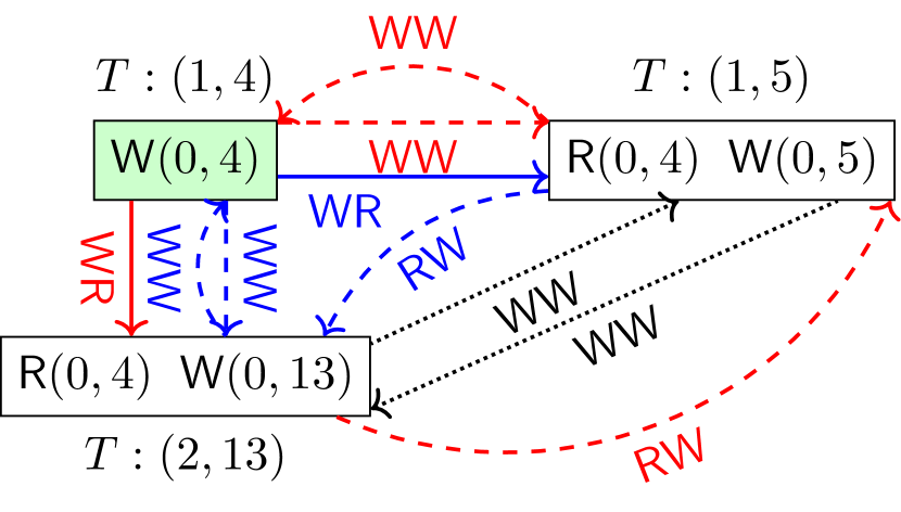
(b) Missing participants

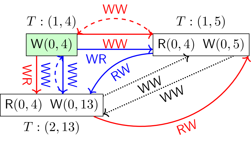
(c) Recovered scenario

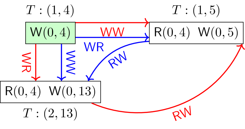
(d) Finalized scenario

Figure 5. Lost update: the SI violation found in MariaDB-Galera. The original output dependencies are represented by dotted black arrows. The recovered dependencies are colored in red/blue with dashed and solid arrows representing uncertain and certain dependencies, respectively. The missing transaction is colored in green. We omit key 0, associated with all dependencies.

Violation Found in MariaDB-Galera. We present an example violation detected in MariaDB-Galera. In particular, we illustrate how the interpretation algorithm helps us locate the violation cause: lost update. We defer the Dgraph and YugabyteDB anomalies (causality violations) to Appendix D. In the following example, we use T:$(s,n)$ to denote the $n$th transaction issued by session $s$.

Given the original cycles returned by MonoSAT in Figure 5(a), PolySI first finds the (only) “missing” transaction T:(1,4) (colored in green) and the associated dependencies, as shown in Figure 5(b). Note that some of the dependencies are uncertain at this moment, e.g., the WW dependency between T:(1,4) and T:(1,5) (in red). PolySI then restores the violating scenario by resolving such uncertainties. For example, as depicted in Figure 5(c), PolySI determines that W(0,4) was actually installed first in the database, i.e., T:(1,4)$\xrightarrow{\textsf{WW}}$T:(1,5), because there would otherwise be an undesired cycle with the known dependencies, i.e., T:(1,5)$\xrightarrow{\textsf{WW}}$T:(1,4)$\xrightarrow{\textsf{WR}}$T:(1,5). The same reasoning applies to determine the WW dependency between T:(1,4) and T:(2,13) (in blue). Finally, PolySI finalizes the violating scenario by removing any remaining uncertainties including those dependencies not involved in the actual violation (the WW dependency between T:(1,5) and T:(2,13) in this case).

The violating scenario now becomes informative and explainable: transaction T:(1,4) writes value 4 on key 0, which is read by transactions T:(2,13) and T:(1,5). Both transactions subsequently commit their writes on key 0 by W(0,13) and W(0,5), respectively, which results in a lost update anomaly.

5.4. Performance Evaluation

In this section, we conduct an in-depth performance analysis of PolySI and compare it to the following black-box checkers:

• dbcop (Biswas and Enea, 2019) is, to the best of our knowledge, the most efficient black-box SI checker that does not use an off-the-shelf solver. Note that, unlike our PolySI tool, dbcop does not check aborted reads or intermediate reads (see Section 4.5).

• Cobra (Tan et al., 2020) is the state-of-the-art SER checker utilizing both MonoSAT and GPUs to accelerate the checking procedure. Cobra serves as a baseline because (i) checking SI is more complicated than checking SER in general (Biswas and Enea, 2019), and constraint pruning and the MonoSAT encoding for SI are more challenging in particular due to more complex cycle patterns in dependency graphs (Theorem 6, Section 2.2.3); and (ii) Cobra is the most performant SER checker to date.

• CobraSI: We implement the incremental algorithm (Biswas and Enea, 2019, Section 4.3) for reducing checking SI to checking serializability (in polynomial time) to leverage Cobra. We consider two variants: (i) CobraSI without GPU for a fair comparison with PolySI and dbcop, which do not employ GPU or multithreading; and (ii) CobraSI with GPU as a strong competitor.

0.23    0.23

0.23    0.23

0.23    0.23

Figure 6. Performance comparison with the competing SI checkers under various workloads. Experiments time out at 180s; data points are not plotted for timed-out experiments.

0.23    0.23

0.23    0.23

0.23    0.23

Figure 7. Comparison on memory overhead with competing SI checkers under various workloads.

0.23    0.23

Figure 8. Comparison on time and memory overhead with Cobra with GPU acceleration under representative workloads.

Figure 9. Decomposing PolySI’s checking time into stages.

Figure 10. Diff. analysis of PolySI. Memory-exhausted runs are colored in red.

5.4.1. Performance Comparison with State of the Art.

Our first set of experiments compares PolySI with the competing SI checkers under a wide range of workloads. The input histories extracted from PostgreSQL (with the repeatable read isolation level) are all valid with respect to SI. The experimental results are shown in Figure 6: PolySI significantly surpasses not only the state-of-the-art SI checker dbcop but also CobraSI with GPU. In particular, with more concurrency, such as more sessions (a), transactions per session (b), and operations per transaction (c), CobraSI with GPU exhibits exponentially increasing checking time while PolySI incurs only moderate overhead. The result depicted in Figure 6(f) is also consistent: with the skewed key accesses representing high concurrency as in the zipfian and hotspot distributions, both dbcop and CobraSI without GPU acceleration time out. Moreover, even with the GPU acceleration, CobraSI takes 6x more time than PolySI. Finally, unlike the other SI checkers, PolySI’s performance is fairly stable with respect to varying read/write proportions (d) and keys (e).

In Figure 8(a) we compare PolySI with the baseline serializability checker Cobra. We present the checking time on various benchmarks. PolySI outperforms Cobra (with its GPU acceleration enabled) in five of the six benchmarks with up to 3x improvement (as for GeneralRH). The only exception is TPC-C, where most of the transactions have the read-modify-write pattern, for which Cobra implements a specific optimization to efficiently infer dependencies before pruning and encoding.

We also measure the memory usage for all the checkers under the same settings as in Figure 6 and Figure 8(a). As shown in Figure 7, PolySI consumes less memory (for storing both generated graphs and constraints) than the competitors in general. Note that dbcop, the only checker that does not rely on solving and stores no constraints, is not competitive with PolySI for most of the cases. Regarding the comparison on specific benchmarks (Figure 8(b)), PolySI and Cobra with GPU acceleration have similar overheads, while PolySI (resp. Cobra) requires less memory for read-heavy workloads (resp. TPC-C).

Table 3. Number of constraints and unknown dependencies before and after pruning (P) in the six benchmarks.

Benchmark	#cons.	#cons.	#unk. dep.	#unk. dep.
	before P	after P	before P	after P
TPC-C	386k	0	3628k	0
GeneralRH	4k	29	39k	77
RUBiS	14k	149	171k	839
C-Twitter	59k	277	307k	776
GeneralRW	90k	2565	401k	5435
GeneralWH	167k	6962	468k	14376

5.4.2. Decomposition Analysis of PolySI

We measure PolySI’s checking time in terms of stages: constructing, which builds up a generalized polygraph from a given history; pruning, which prunes constraints in the generalized polygraph; encoding, which encodes the graph and the remaining constraints; and solving, which runs the MonoSAT solver.

Figure 10 depicts the results on six different datasets. Constructing a generalized polygraph is relatively inexpensive. The overhead of pruning is fairly constant, regardless of the workloads; PolySI can effectively prune (resp. resolve) a huge number of constraints (resp. unknown dependencies) in this phase. See Table 3 for details. In particular, for TPC-C which contains only read-only and read-modify-write transactions, PolySI is able to resolve all uncertainties on WW relations and identify the unique version chain for each key. The encoding effort is moderate; TPC-C incurs more overhead as the number of operations in total is 5x more than the others. The solving time depends on the remaining constraints and unknown dependencies after pruning, e.g., the left four datasets incur negligible overhead (see Table 3).

5.4.3. Differential Analysis of PolySI

To investigate the contributions of PolySI’s two major optimizations, we experiment with three variants: (i) PolySI itself; (ii) PolySI without pruning (P) constraints; and (iii) PolySI without both compacting (C) and pruning the constraints. Figure 10 demonstrates the acceleration produced by each optimization. Note that the two variants without optimization exhibit (16GB) memory-exhausted runs on TPC-C, which contain considerably more uncertain dependencies (3628k) and constraints (386k) without pruning than the other datasets (see Table 3).

5.4.4. Scalability.

To assess PolySI’s scalability, we generate transaction workloads with one billion keys and one million transactions with hundreds of millions of operations. We experiment with varying read proportions and long transaction sizes (up to 450 operations per transaction). As shown in Figure 11, PolySI consumes less than 40GB memory in all cases and at most 4 hours for checking one million transactions. We also observe that the time used increases linearly with larger-sized transactions while the memory overhead is fairly stable. To conclude, large-sized workloads are quite manageable for PolySI on modern hardware. Note that the competing checkers, as expected, fail to handle such workloads.

0.20      0.20

0.20      0.20

Figure 11. PolySI’s overhead on large-sized workloads with one billion keys and one million transactions.

6. Discussion

Fault Injection. We have found SI violations in three production databases without injecting faults, such as network partition and clock drift. Since PolySI is an off-the-shelf checker, it is straightforward to integrate it into existing testing frameworks with fault injection such as Jepsen (Jepsen, 2022a) and CoFI (Chen et al., 2020); both have been demonstrated to effectively trigger bugs in distributed systems.

Database Schema. In our testing of production databases, we used a simple, yet effective, database schema adopted by most of black-box checkers (Zellag and Kemme, 2014; Biswas and Enea, 2019; Zennou et al., 2019; Tan et al., 2020): a two-column table storing key-value pairs. Extending it to multi-columns or even the column-family data model could be done by: (i) representing each cell in a table as a compound key, i.e., “TableName:PrimaryKey:ColumnName”, and a single value, i.e., the content of the cell (Lloyd et al., 2013; Biswas et al., 2021); and (ii) utilizing the compiler in (Biswas et al., 2021) to rewrite (more complex) SQL queries to key-value read/write operations.

Predicates. To the best of our knowledge, none of the state-of-the-art black-box checkers (Zellag and Kemme, 2014; Biswas and Enea, 2019; Zennou et al., 2019; Tan et al., 2020; Kingsbury and Alvaro, 2020; Biswas et al., 2021) considers predicates nor can they detect predicate-specific anomalies. Given the non-predicate violations found by PolySI (as well as dbcop (Biswas and Enea, 2019) and Elle (Kingsbury and Alvaro, 2020)), we conjecture that more anomalies would arise with predicates. It is therefore interesting future work to extend our SI characterization to represent predicates and to explore optimizations with respect to encoding and pruning.

Unique Value. As demonstrated in our experiments, guaranteeing “unique value” is a pragmatic, purely black-box technique, and effective in detecting anomalies. When this assumption is broken, the complexity of the checking problem would become higher due to inferring uncertain WR dependencies (a single read may be related to multiple “false” writes). Accordingly, we could add the encoding in PolySI for unique existence of WR dependency among all uncertainties prior to SAT solving.

Optimization for Long Histories. PolySI’s overhead when checking one million transactions with 450 operations per long transaction is manageable for modern hardware. Still, optimizing PolySI for long transaction histories would help to reduce checking overhead, especially for online transactional processing workloads. We could consider periodically taking snapshots (via read-only transactions) across all sessions in a history using an additional client session. Such snapshots carry the summary of write dependencies thus far, which discards prior transactions in the history. As a result, at any point of time, one only needs to consider a segment of the history consisting of the latest snapshot and its subsequent transactions.

7. Related Work

Characterizing Snapshot Isolation. Many frameworks and formalisms have been developed to characterize SI and its variants. Berenson et al.  (Berenson et al., 1995) considers SI as a multi-version concurrency control mechanism (described also in Section 2.1). Adya (Adya, 1999) presents the first formal definition of SI using dependency graphs, which, as pointed out by (Cerone and Gotsman, 2018), still relies on low-level implementation choices such as how to order start and commit events in transactions. Cerone et al. (Cerone et al., 2015) proposes an axiomatic framework to declaratively define SI with the dual notions of visibility (what transactions can observe) and arbitration (the order of installed versions/values). The follow-up work (Cerone and Gotsman, 2018) characterizes SI solely in terms of Adya’s dependency graphs, requiring no additional information about transactions. Crooks et al. (Crooks et al., 2017) introduces an alternative implementation-agnostic formalization of SI and its variants based on client-observed values read/written.

Driven by black-box testing of SI, we base our GP-based characterization on Cerone and Gotsman’s formal specification (Cerone and Gotsman, 2018). In particular, our new characterization:

(i) targets the prevalent strong session variant of SI (Cerone and Gotsman, 2018; Daudjee and Salem, 2006), where sessions, advocated by Terry et al. (Terry et al., 1994), have been adopted by many production databases in practice (e.g., DGraph (Dgraph, 2022), Galera (Cluster, 2022), and CockroachDB (CockroachDB, 2022));

(ii) does not rely on implementation details such as concurrency control mechanism as in (Berenson et al., 1995) and timestamps as in (Adya, 1999), and the operational semantics of the underlying database as in (Xiong et al., 2020), which are usually invisible to the outsiders; and

(iii) naturally models uncertain dependencies inherent to black-box testing using generalized constraints (Section 3) and enables the acceleration of SMT solving by compacting constraints (Section 5.4).

Regarding the comparison with (Crooks et al., 2017), despite its promising characterization of SI suitable for black-box testing, we are unaware of any checking algorithm based on it. A straightforward (suboptimal) implementation would require enumerating all permutations of the transactions in a history, e.g., 10k transactions in our experiment would require checking 10k-factorial permutations.

Dynamic Checking of SI. This technique determines whether a collected history from dynamically executing a database satisfies SI. We are unaware of any black-box SI checker that satisfies SIEGE+.

dbcop (Biswas and Enea, 2019) is the most efficient black-box SI checker to date. The underlying checking algorithm runs in time $O(n^{c})$, with $n$ and $c$ the number of transactions and clients involved in a single history, respectively. The authors devise both a polynomial-time algorithm for checking serializabilty (also with a fixed number of client sessions) and a polynomial-time algorithm for reducing checking SI to checking serializabilty. However, as demonstrated in Section 5.4, dbcop is practically not as efficient as our PolySI tool under various workloads. Moreover, dbcop is incomplete as it does not check non-cycle anomalies such as aborted reads and intermediate reads (Section 4.5). Finally, dbcop provides no details upon a violation; only a “false” answer is returned.

Elle (Kingsbury and Alvaro, 2020) is a state-of-the-art checker for a variety of isolation levels, including strong session SI, which is part of the Jepsen (Jepsen, 2022a) testing framework. Elle requires specific data models like lists in workloads to infer the WW dependencies and specific APIs to perform list-specific operations such as “append”. In contrast, PolySI is compatible with general and production workloads and uses standard key-value and SQL APIs. Elle builds upon Adya’s formalization of SI (Adya, 1999), thus relying on the start and commit timestamps of transactions for completeness. Such information may not always be available, e.g., MongoDB (MongoDB, 2022) and TiDB (TiDB, 2022) have no timestamps in their logs for read-only transactions. Nonetheless, the underlying SI characterization for PolySI does not rely on any implementation details. Finally, Elle’s actual implementation is incomplete for efficiency reasons and there are anomalies it cannot detect. We have confirmed this with the developer (Huang et al., 2022).

ConsAD (Zellag and Kemme, 2014) is a checker tailored to application servers as opposed to black-box databases in our setting. Its SI checking algorithm is also based on dependency graphs. To determine the WW dependencies, ConsAD enforces the commit order of update transactions using, e.g., artificial SQL queries, to acquire exclusive locks on the database records, resulting in additional overhead (Zellag and Kemme, 2014; Shang et al., 2018). Moreover, ConsAD is incapable of detecting non-cycle anomalies.

CAT (Liu et al., 2019) is a dynamic white-box checker for SI (and several other isolation levels). The current release is restricted to distributed databases implemented in the Maude formal language (Clavel et al., 2007). CAT must capture the internal transaction information, e.g., start/commit times, during a system run.

8. Conclusion

We have presented the design of PolySI, along with a novel characterization of SI using generalized polygraphs. We have established the soundness and completeness of our new characterization and PolySI’s checking algorithm. Moreover, we have demonstrated PolySI’s effectiveness by reproducing all of 2477 known anomalies and by finding new violations in three popular production databases, its efficiency by experimentally showing that it outperforms the state-of-the-art tools and can scale up to large-sized workloads, and its generality, operating over a wide range of workloads and databases of different kinds. Finally, we have leveraged PolySI’s interpretation algorithm to identify the causes of the violations.

PolySI is the first black-box SI checker that satisfies the SIEGE+ principle. The obvious next step is to apply SMT solving to build SIEGE+ black-box checkers for other data consistency properties such as transactional causal consistency (Lloyd et al., 2013; Didona et al., 2018) and the recently proposed regular sequential consistency (Helt et al., 2021). Moreover, we will pursue the research directions discussed in Section 6.

Appendix A The Checking Algorithm for SI

Algorithm 2 The PolySI algorithm for checking SI (the full version)

1:procedure CheckSI($\mathcal{H}$)

2:    if $\mathcal{H}\not\models\textsc{Int}\lor\textsc{AbortedReads}\lor\textsc{IntermediateReads}$ 

3:        return false    

4:    CreateKnownGraph($\mathcal{H}$)

5:    GenerateConstraints($\mathcal{H}$)

6:    if $\lnot\textsc{{PruneConstraints}}(\hbox{})$ 

7:        return false     

8:    SAT-Encode()

9:    return MonoSAT-Solve()

10:

11:procedure CreateKnownGraph($\mathcal{H}$)

12:    for all $T,S\in\mathcal{T}$ such that $T\xrightarrow{\textsf{SO}}S$ 

13:        $\mathit{E}_{\mathit{G}}\leftarrow\mathit{E}_{\mathit{G}}\cup(T,S,\textsf{SO})$     

14:    for all $T,S\in\mathcal{T}$ such that $T\xrightarrow{\textsf{WR}}S$ 

15:        $\mathit{E}_{\mathit{G}}\leftarrow\mathit{E}_{\mathit{G}}\cup(T,S,\textsf{WR})$     

16:

17:procedure GenerateConstraints($\mathcal{H}$)

18:    for all $\mathit{x}\in{\sf Key}$ 

19:        for all $T,S\in{\sf WriteTx}_{\mathit{x}}$ such that $T\neq S$ 

20:           $\mathit{either}\leftarrow\{(T,S,\textsf{WW})\}\cup\bigcup\limits_{T^{\prime}\in\textsf{WR}(\mathit{x})(T)}\!\!\{(T^{\prime},S,\textsf{RW})\}$

21:           $\mathit{or}\leftarrow\{(S,T,\textsf{WW})\}\cup\bigcup\limits_{S^{\prime}\in\textsf{WR}(\mathit{x})(S)}\!\!\{(S^{\prime},T,\textsf{RW})\}$

22:           $\mathit{C}_{\mathit{G}}\leftarrow\mathit{C}_{\mathit{G}}\cup\{\langle\mathit{either},\mathit{or}\rangle\}$             

23:

24:procedure SAT-Encode()

25:    for all $\mathit{v}_{i},\mathit{v}_{j}\in\mathit{V}_{\mathit{G}}$ such that $i\neq j$ 

26:        Create two Boolean variables $\mathsf{BV}_{i,j}$ and $\mathsf{BV}^{\mathit{I}}_{i,j}$

27:        $\mathsf{BV}\leftarrow\mathsf{BV}\cup\{\mathsf{BV}_{i,j},\mathsf{BV}^{\mathit{I}}_{i,j}\}$     

28:    for all $(\mathit{v}_{i},\mathit{v}_{j})\in\mathit{E}_{\mathit{G}}$  $\triangleright$ encode the known graph $\mathit{G}$

29:        $\mathsf{CL}\leftarrow\mathsf{CL}\cup\{\mathsf{BV}_{i,j}=\textsf{True}\}$     

30:    for all $\langle\mathit{either},\mathit{or}\rangle\in\mathit{C}_{\mathit{G}}$  $\triangleright$ encode the constraints $\mathit{G}$

31:        $\mathsf{CL}\leftarrow\mathsf{CL}\;\cup\;\bigg{\{}\bigl{(}\bigwedge\limits_{(\mathit{v}_{i},\mathit{v}_{j},\_)\in\mathit{either}}\mathsf{BV}_{i,j}\land\bigwedge\limits_{(\mathit{v}_{i},\mathit{v}_{j},\_)\in\mathit{or}}\lnot\mathsf{BV}_{i,j}\bigr{)}\;\lor\;\bigl{(}\bigwedge\limits_{(\mathit{v}_{i},\mathit{v}_{j},\_)\in\mathit{or}}\mathsf{BV}_{i,j}\land\bigwedge\limits_{(\mathit{v}_{i},\mathit{v}_{j},\_)\in\mathit{either}}\lnot\mathsf{BV}_{i,j}\bigr{)}\bigg{\}}$     

32:    $\mathit{Dep}\leftarrow\mathit{G}|_{\textsf{SO}_{\mathit{G}}\cup\textsf{WR}_{\mathit{G}}\cup\textsf{WW}_{\mathit{G}}}$

33:    $\mathit{E}_{\mathit{Dep}}\leftarrow\mathit{E}_{\mathit{Dep}}\cup\{(\_,\_,\textsf{WW})\in\mathit{either}\cup\mathit{or}\mid\langle\mathit{either},\mathit{or}\rangle\in\mathit{C}_{\mathit{G}}\}$

34:    $\mathit{AntiDep}\leftarrow\mathit{G}|_{\textsf{RW}_{\mathit{G}}}$

35:    $\mathit{E}_{\mathit{AntiDep}}\leftarrow\mathit{E}_{\mathit{AntiDep}}\cup\{(\_,\_,\textsf{RW})\in\mathit{either}\cup\mathit{or}\mid\langle\mathit{either},\mathit{or}\rangle\in\mathit{C}_{\mathit{G}}\}$

36:    $\mathsf{CL}\leftarrow\mathsf{CL}\cup\bigg{\{}\mathsf{BV}^{\mathit{I}}_{i,j}=\big{(}\mathsf{BV}_{i,j}\land(\mathit{v}_{i},\mathit{v}_{j},\_)\in\mathit{E}_{\mathit{Dep}}\big{)}\lor\big{(}\bigvee\limits_{\begin{subarray}{c}(\mathit{v}_{i},\mathit{v}_{k},\_)\in\mathit{E}_{\mathit{Dep}}\\ (\mathit{v}_{k},\mathit{v}_{j},\_)\in\mathit{E}_{\mathit{AntiDep}}\end{subarray}}\mathsf{BV}_{i,k}\land\mathsf{BV}_{k,j}\big{)}\bigm{|}\mathit{v}_{i},\mathit{v}_{j}\in\mathit{V}_{\mathit{G}}\bigg{\}}$ $\triangleright$ encode the induced SI graph $\mathit{I}$ of $\mathit{G}$

37:procedure PruneConstraints()

38:    repeat

39:        $\mathit{Dep}\leftarrow\mathit{G}|_{\textsf{SO}_{\mathit{G}}\cup\textsf{WR}_{\mathit{G}}\cup\textsf{WW}_{\mathit{G}}}$

40:        $\mathit{AntiDep}\leftarrow\mathit{G}|_{\textsf{RW}_{\mathit{G}}}$

41:        $\mathit{KI}\leftarrow\mathit{Dep}\cup(\mathit{Dep}\;;\;\mathit{AntiDep})$

42:        $\mathit{reachability}\leftarrow\textsc{{Reachability}}(\mathit{KI})$

43:        for all $\mathit{cons}\leftarrow\langle\mathit{either},\mathit{or}\rangle\in\mathit{C}_{\mathit{G}}$ 

44:           for all $(\mathit{from},\mathit{to},\mathit{type})\in\mathit{either}$  $\triangleright$ for the “$\mathit{either}$” possibility

45:               if $\mathit{type}=\textsf{WW}$ 

46:                  if $(\mathit{to},\mathit{from})\in\mathit{reachability}$ 

47:                      $\mathit{C}_{\mathit{G}}\leftarrow\mathit{C}_{\mathit{G}}\setminus\{\mathit{cons}\}$

48:                      $\mathit{E}_{\mathit{G}}\leftarrow\mathit{E}_{\mathit{G}}\cup\mathit{or}$

49:                      break the “for all $(\mathit{from},\mathit{to},\mathit{type})\in\mathit{either}$” loop                   

50:               else$\triangleright$ $\mathit{type}=\textsf{RW}$

51:                  for all $\mathit{prec}\in\mathit{V}_{\mathit{Dep}}$ such that $(\mathit{prec},\mathit{from},\_)\in\mathit{E}_{\mathit{Dep}}$ 

52:                      if $(\mathit{to},\mathit{prec})\in\mathit{reachability}$ 

53:                          $\mathit{C}_{\mathit{G}}\leftarrow\mathit{C}_{\mathit{G}}\setminus\{\mathit{cons}\}$

54:                          $\mathit{E}_{\mathit{G}}\leftarrow\mathit{E}_{\mathit{G}}\cup\mathit{or}$

55:                          break the “for all $(\mathit{from},\mathit{to},\mathit{type})\in\mathit{either}$” loop                                                                   

56:           for all $(\mathit{from},\mathit{to},\mathit{type})\in\mathit{or}$  $\triangleright$ for the “$\mathit{or}$” possibility

57:               if $\mathit{type}=\textsf{WW}$ 

58:                  if $(\mathit{to},\mathit{from})\in\mathit{reachability}$ 

59:                      if $\mathit{cons}\notin\mathit{C}_{\mathit{G}}$  $\triangleright$ neither “$\mathit{either}$” nor “$\mathit{or}$” is possible

60:                          return False                       

61:                      $\mathit{C}_{\mathit{G}}\leftarrow\mathit{C}_{\mathit{G}}\setminus\{\mathit{cons}\}$

62:                      $\mathit{E}_{\mathit{G}}\leftarrow\mathit{E}_{\mathit{G}}\cup\mathit{either}$

63:                      break the “for all $(\mathit{from},\mathit{to},\mathit{type})\in\mathit{or}$” loop                   

64:               else$\triangleright$ $\mathit{type}=\textsf{RW}$

65:                  for all $\mathit{prec}\in\mathit{V}_{\mathit{Dep}}$ such that $(\mathit{prec},\mathit{from},\_)\in\mathit{E}_{\mathit{Dep}}$ 

66:                      if $(\mathit{to},\mathit{prec})\in\mathit{reachability}$ 

67:                          if $\mathit{cons}\notin\mathit{C}_{\mathit{G}}$  $\triangleright$ neither “$\mathit{either}$” nor “$\mathit{or}$” is possible

68:                             return False                           

69:                          $\mathit{C}_{\mathit{G}}\leftarrow\mathit{C}_{\mathit{G}}\setminus\{\mathit{cons}\}$

70:                          $\mathit{E}_{\mathit{G}}\leftarrow\mathit{E}_{\mathit{G}}\cup\mathit{either}$

71:                          break the “for all $(\mathit{from},\mathit{to},\mathit{type})\in\mathit{or}$” loop                                                                           

72:    until $\mathit{C}_{\mathit{G}}$ remains unchanged

73:    return True

74:

75:procedure MonoSAT-Solve()

76:    $\mathit{solver}\leftarrow\textsc{{MonoSAT-Solver}}(\mathsf{BV},\mathsf{CL})$

77:    return $\textsc{{Solve}}(\mathit{solver},\mathit{I}\text{ is acyclic})$

The full version of the checking algorithm is given in Algorithm 2. In the following, we reference pseudocode lines using the format algorithm#:line#.

Appendix B Proofs

B.1. Proof of Theorem 8

Proof.

The proof proceeds in two directions.

(“$\implies$”) Suppose that $\mathcal{H}$ satisfies SI. By Theorem 6, $\mathcal{H}$ satisfies Int and there exist WR, WW, and RW relations with which $\mathcal{H}$ can be extended to a dependency graph $G$ such that $(\textsf{SO}_{\mathit{G}}\cup\textsf{WR}_{\mathit{G}}\cup\textsf{WW}_{\mathit{G}})\;;\;\textsf{RW}_{\mathit{G}}?$ is acyclic. We show that the generalized polygraph $G^{\prime}$ of $\mathcal{H}$ is SI-acyclic by constructing a compatible graph $G^{\prime\prime}$ with $G^{\prime}$ such that $G^{\prime\prime}|_{\mathcal{R}}$ is acyclic when the edge types are ignored: Consider a constraint $\langle\mathit{either},\mathit{or}\rangle$ in $G^{\prime}$ and any WW edge $T\xrightarrow{\textsf{WW}}S$ in $G$. If $(T,S,\textsf{WW})\in\mathit{either}$, add all the edges in $\mathit{either}$ into $G^{\prime\prime}$. Otherwise, add all the edges in $\mathit{or}$ into $G^{\prime\prime}$.

(“$\impliedby$”) Suppose that $\mathcal{H}\models\textsc{Int}$ and the generalized polygraph $G^{\prime}$ of $\mathcal{H}$ is SI-acyclic. By Definition 7, there exists a compatible graph $G^{\prime\prime}$ with $G^{\prime}$ such that $G^{\prime\prime}|_{\mathcal{R}}$ is acyclic when the edge types are ignored. We show that $\mathcal{H}$ satisfies SI by constructing suitable WR, WW, and RW relations with which $\mathcal{H}$ can be extended to a dependency graph $G$ such that $(\textsf{SO}_{\mathit{G}}\cup\textsf{WR}_{\mathit{G}}\cup\textsf{WW}_{\mathit{G}})\;;\;\textsf{RW}_{\mathit{G}}?$ is acyclic: We simply take $G$ to be $G^{\prime\prime}$ by defining, e.g., $\textsf{WW}=\{(a,b)\mid(a,b,\textsf{WW})\in E_{G^{\prime\prime}}\}$. ∎

B.2. Proof of Theorem 1

Proof.

We prove (1) by induction on the number of iterations of pruning. Consider an arbitrary iteration of pruning $\mathcal{P}$ (lines 2:39–2:71) and denote the generalized polygraphs just before and after $\mathcal{P}$ by $G_{1}$ and $G_{2}$, respectively. We should show that $G_{1}$ is SI-acyclic if and only if $\mathcal{P}$ does not return False from line 2:60 or line 2:68 and $G_{2}$ is SI-acyclic. The following proof proceeds in two directions.

(“$\implies$”) Suppose that $G_{1}$ is SI-acyclic. We then proceed by contradiction.

• Suppose that $\mathcal{P}$ returns False from line 2:60 or line 2:68. This happens when some constraint in $G_{1}$ constructed based on two write transactions, say $T$ and $S$, on the same key cannot be resolved appropriately: every compatible graph with the induced SI graph of $G_{1}$ contains a cycle without adjacent RW edges, no matter whether $T\xrightarrow{\textsf{WW}}S$ or $S\xrightarrow{\textsf{WW}}T$ is in it. That is, $G_{1}$ is not SI-acyclic. Contradiction.

• Suppose that $G_{2}$ is not SI-acyclic. $G_{1}$ is not SI-acyclic because the set of constraints in $G_{2}$ is a subset of that in $G_{1}$ and $\mathcal{P}$ prunes a constraint only if one of its two possibilities cannot happen. Contradiction.

(“$\impliedby$”) Suppose that $\mathcal{P}$ does not return False from line 2:60 or line 2:68 and $G_{2}$ is SI-acyclic. Therefore, there exists an acyclic compatible graph with the induced SI graph of $G_{2}$. This is also an acyclic compatible graph with the induced SI graph of $G_{1}$. Hence, $G_{1}$ is SI-acyclic.

The second part of the theorem holds because any compatible graph with the induced SI graph of $G_{p}$ is also a compatible graph with the induced SI graph of $G$. ∎

Appendix C The Interpretation Algorithm

In this section, we describe the interpretation algorithm, called Interpret, that helps locate the causes of violations found by PolySI; see Algorithm 3. The algorithm takes as input the undesired cycles constructed from the log generated by MonoSAT, and outputs a dependency graph demonstrating the cause of the violation.

Algorithm 3 The interpretation algorithm.

1:$\mathcal{H}=(\mathcal{T},\textsf{SO})$: the original history

2:$G=(\mathit{V}\_1,\mathit{E}\_1,\mathit{C}\_1)$: the polygraph

3:$\mathcal{C}=(\mathit{V}\_2,\mathit{E}\_2)$: The cycle found by PolySI

4:

5:procedure Interpret($\mathcal{H},G,\mathcal{C}$)

6:    $\mathit{Graph_{recovered}}$ $\leftarrow$ $\textsc{{Restore}}(\mathcal{H},G,\mathcal{C})$

7:    $\mathit{Graph_{tagged}}$ $\leftarrow$ $\textsc{{Resolve}}(\mathit{Graph_{recovered}},\mathcal{H},G,\mathcal{C})$

8:    $\mathit{Graph_{finalized}}$ $\leftarrow$ $\textsc{{Finalize}}(\mathit{Graph_{tagged}})$

9:    return $\mathit{Graph_{recovered}},\mathit{Graph_{tagged}},\mathit{Graph_{finalized}}$

10:

11:procedure Restore($\mathcal{H},G,\mathcal{C}$)

12:    $\mathit{Graph_{recovered}}\leftarrow\textsc{{Find\_ACS}}(\mathcal{C})$

13:    for all $(u\xrightarrow{\textsf{RW}}v)\in\mathit{E}\_2$ 

14:        for all $c\in\mathit{C}\_1$ 

15:           if $((u\xrightarrow{\textsf{RW}}v)\in\mathit{c})\wedge(\exists w,(w\xrightarrow{\textsf{WW}}v)\in\mathit{c})$ 

16:               $\mathit{Graph_{recovered}}$ $\leftarrow$ $\mathit{Graph_{recovered}}\cup\{w\xrightarrow{\textsf{WW}}v\}\cup\{w\xrightarrow{\textsf{WR}}u\}$                        

17:    return $\mathit{Graph_{recovered}}$

18:

19:procedure Find_ACS($\mathit{Graph_{acs}},G$)

20:    $\mathit{graph\_size}$ $\leftarrow$ number of edges in $\mathit{Graph_{acs}}$

21:    $\mathit{minimal\_extend\_deps}$ $\leftarrow$ $+\infty$

22:    $\mathit{minimal\_acs}$ $\leftarrow$ empty

23:    for all $\mathit{dep}\in(\mathit{E}\_2\cap\mathit{c}.either)$, where $\mathit{c}\in\mathit{C}\_1$ 

24:        if ($\exists\mathit{dep}^{\prime}\in\mathit{c}.or,\mathit{dep}^{\prime}\in\mathit{Graph_{recovered}}$)  continue         

25:        for all $\mathit{dep}^{\prime}\in\mathit{c}.or$ 

26:           for all ( cycle $(\mathit{V}^{\prime},\mathit{E}^{\prime})\subseteq G$) $\wedge$ ($\mathit{dep}^{\prime}\in\mathit{E}^{\prime}$ ) 

27:               $\mathit{Graph_{tested}}$ $\leftarrow$ $\mathit{Graph_{recovered}}\cup(\mathit{V}^{\prime},\mathit{E}^{\prime})$

28:               $(\mathit{extendDeps},\mathit{extendDeps})$ $\leftarrow$ $\textsc{{Find\_ACS}}(\mathit{Graph_{tested}},G)$

29:               if $\mathit{extendDeps}<\mathit{minimal\_extend\_deps}$ 

30:                  $\mathit{minimal\_extend\_deps}$ $\leftarrow$ $\mathit{extendDeps}$

31:                  $\mathit{minimal\_acs}$ $\leftarrow$ $\mathit{graph_{extended}}$                                       

32:    for all $\mathit{dep}\in(\mathit{E}\_2\cap\mathit{c}.or)$, where $\mathit{c}\in\mathit{C}\_1$ 

33:        if ($\exists\mathit{dep}^{\prime}\in\mathit{c}.either,\mathit{dep}^{\prime}\in\mathit{Graph_{recovered}}$)  continue         

34:        for all $\mathit{dep}^{\prime}\in\mathit{c}.either$ 

35:           for all ( cycle $(\mathit{V}^{\prime},\mathit{E}^{\prime})\subseteq G$) $\wedge$ ($\mathit{dep}^{\prime}\in\mathit{E}^{\prime}$ ) 

36:               $\mathit{Graph_{tested}}$ $\leftarrow$ $\mathit{Graph_{recovered}}\cup(\mathit{V}^{\prime},\mathit{E}^{\prime})$

37:               $(\mathit{extendDeps},\mathit{extendDeps})$ $\leftarrow$ $\textsc{{Find\_ACS}}(\mathit{Graph_{tested}},G)$

38:               if $\mathit{extendDeps}<\mathit{minimal\_extend\_deps}$ 

39:                  $\mathit{minimal\_extend\_deps}$ $\leftarrow$ $\mathit{extendDeps}$

40:                  $\mathit{minimal\_acs}$ $\leftarrow$ $\mathit{graph_{extended}}$                                        return $(\mathit{minimal\_extend\_deps},\mathit{minimal\_acs}+\mathit{graph\_size})$

41:procedure Resolve($\mathit{Graph_{recovered}},\mathcal{H},G,\mathcal{C}$)

42:    $\mathit{Graph_{tagged}}\leftarrow\mathit{Graph_{recovered}}$

43:    for all $\mathit{dep}\in\mathit{Graph_{tagged}}$ 

44:        if $\mathit{dep}\in\mathit{E}\_1$ 

45:           $\mathit{dep}.tag$ $\leftarrow$ ‘certain’

46:        else

47:           $\mathit{dep}.tag$ $\leftarrow$ ‘uncertain’             

48:    while $\mathit{Graph_{tagged}}$ was changed in the last loop 

49:        for all $\mathit{dep}\in\mathit{Graph_{tagged}}$ 

50:           if ($\mathit{dep}.tag$ = ‘uncertain’) $\wedge$ ($\mathit{dep}$ in a cycle $(\mathit{V}^{\prime},\mathit{E}^{\prime})$) 

51:               if $\forall\mathit{dep}^{\prime}\in\mathit{E}^{\prime}\wedge\mathit{dep}^{\prime}\neq\mathit{dep}$, $\mathit{dep}^{\prime}.tag$ = certain  

52:                  $\mathit{dep}.tag$ $\leftarrow$ ‘uncertain’

53:                  for all $\mathit{dep}_{opposite}$, where $\{\mathit{dep}/\mathit{dep}_{opposite}\}\in\mathit{C}\_1$ 

54:                      $\mathit{dep}_{opposite}.tag$ $\leftarrow$ ‘certain’                                                          return $\mathit{Graph_{tagged}}$

55:

56:procedure Finalize($\mathit{Graph_{tagged}}$)

57:    $\mathit{Graph_{finalized}}$ $\leftarrow$ $\mathit{Graph_{tagged}}$

58:    for all $\mathit{dep}\in\mathit{Graph_{finalized}}$ 

59:        if $\mathit{dep}.tag=$ ‘uncertain’ 

60:           $\mathit{Graph_{finalized}}$ $\leftarrow$ $\mathit{Graph_{finalized}}\setminus\{\mathit{dep}\}$             

61:    return $\mathit{Graph_{finalized}}$

It is often difficult to locate the cause of a violation based solely on the original cycles because the cycles may miss some crucial information such as the core participating transactions and the dependencies between transactions. Therefore, Interpret first restores such information from the generalized polygraph of the history to reproduce the whole violating scenario (line 3:6). This may bring uncertain dependencies to the resulting polygraph, which are then resolved via pruning (line 3:7). Finally, Interpret finalizes the violating scenario by removing any remaining uncertain dependencies, as they are the “effect” of the violation instead of the “cause” (line 3:8).

Restore Transactions and Dependencies.

The procedure Restore restores dependencies and the transactions involved in these dependencies in two steps (line 3:11). First, it checks each RW dependency in the input undesired cycles and restores its associated WW and WR dependencies if they are missing (lines 3:13 – 3:16). Then, for each WW dependency in an undesired cycle, it restores the other direction of this WW dependency (if missing) which may be involved in another undesired cycle (line 3:23 - line 3:40). Now it has recovered the minimal counter example. To help understand the violation more clearly, it checks each RW dependency in the input undesired cycles and restore its associated WW and WR dependencies if they are missing ((line 3:13 – 3:16).

Resolve Uncertain Dependencies.

The restored violating scenario may contain WW and RW dependencies that are still uncertain at this moment. For an uncertain dependency to be part of the cause of a violation, it must be resolved. The procedure Resolve resolves as many uncertain dependencies as possible using the same idea of pruning (Section 4.3). Specifically, if an uncertain dependency from $\mathit{either}$ (resp. $\mathit{or}$) in a constraint would create an undesired cycle with other certain dependencies, it, along with its associated dependencies in $\mathit{either}$ (resp. $\mathit{or}$) is removed and the dependencies in $\mathit{or}$ (resp. $\mathit{either}$) become certain (lines 3:48 -  3:54).

Finalize the Violating Scenario.

The procedure Finalize finalizes the violating scenario by removing all the remaining uncertain dependencies, as they are the “effect” of the violation instead of the “cause” (line 3:56).

Appendix D Causality Violations Found

D.1. A Causality Violation Found in Dgraph

(a) Original output

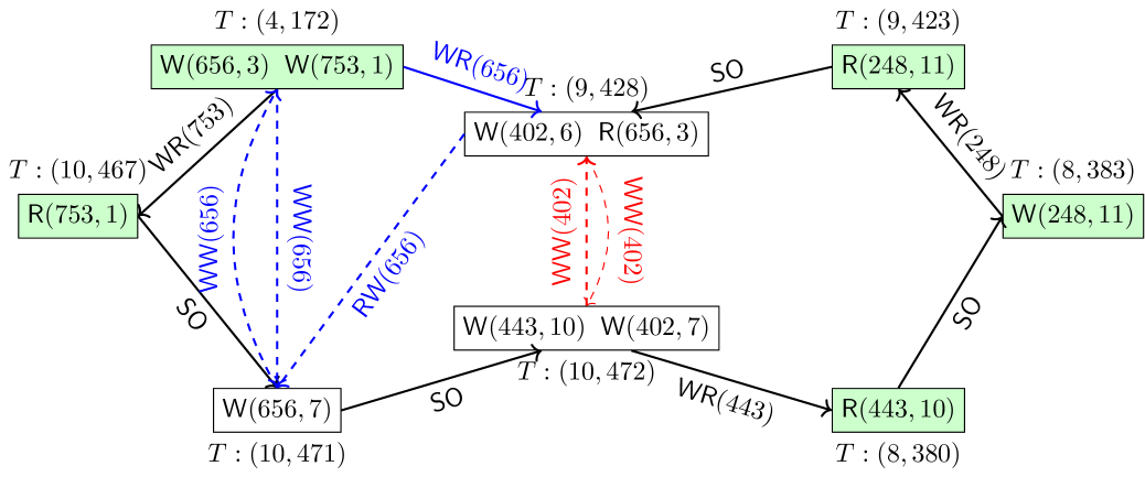
(b) Missing participants

(c) Recovered scenario

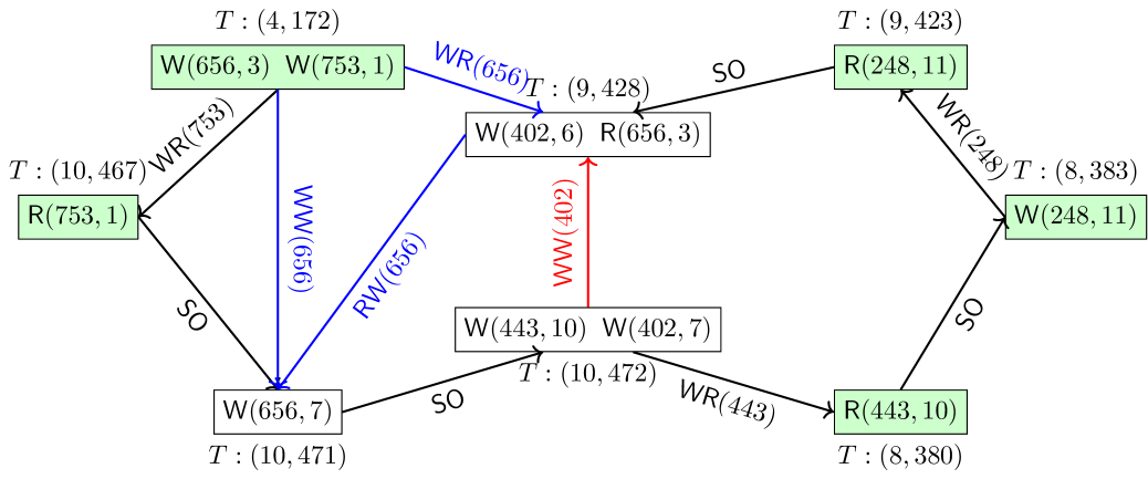
(d) Finalized scenario

Figure 12. Causality violation: the SI anomaly found in Dgraph. Dashed and solid arrows represent uncertain and certain dependencies, respectively. Recovered transactions are colored in green. The core dependencies involved in the two sub-scenarios are colored in red and blue, respectively.

There might be multiple “missing” transactions that together contribute to a violation. As depicted in Figure 12(b), PolySI restores the potentially involved five transactions (in green) and the associated dependencies from the original output cycle in Figure 12(a). In particular, two sub-scenarios are involved: the left subgraph concerns the $\textsf{RW}(656)$ dependency on key 656 (in blue) while the right subgraph concerns the dependency $\textsf{WW}(402)$ on key 402 (in red). Following the same procedure as in the MariaDB-Galera example, PolySI resolves the outstanding dependencies if no undesired cycles arise; see Figure 12(c). For example, we have T:(4,172)$\xrightarrow{\textsf{WW}}$T:(10,471) (in blue) as there would otherwise be a cycle T:(10,471)$\xrightarrow{\textsf{WW}}$T:(4,172)$\xrightarrow{\textsf{WR}}$T:(10,467)$\xrightarrow{\textsf{SO}}$T:(10,471). The final violating scenario is shown in Figure 12(d) where two impossible (dashed) dependencies in Figure 12(c) have been eliminated.

This violation occurs as the causality order is violated, which is a happens-before relationship between any two transactions in a given history (Lamport, 1978; Lloyd et al., 2013). More specifically, transaction T:(9,428) causally depends on transaction T:(10,471) (via the counterclockwise path in the right subgraph) and transaction T:(10,471) causally depends on transaction T:(4,172) (via the clockwise path in the left subgraph). Hence, transaction T:(9,428) should have fetched the value 7 of key 656 written by transaction T:(10,471), instead of the value 3 of transaction T:(4,172), to respect the causality order.

D.2. A Causality Violation Found in YugabyteDB

(a) Original output

(b) Missing participants

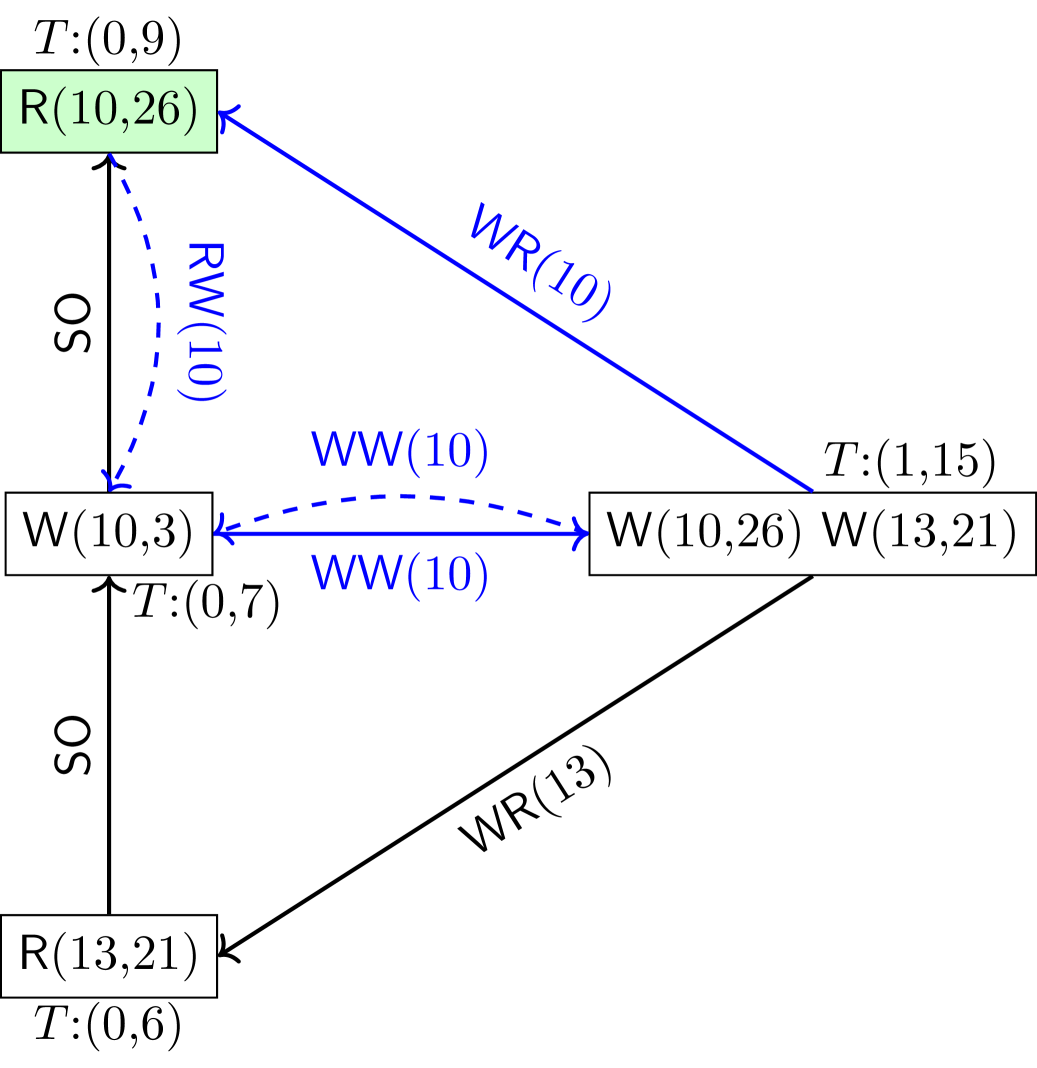
(c) Recovered scenario

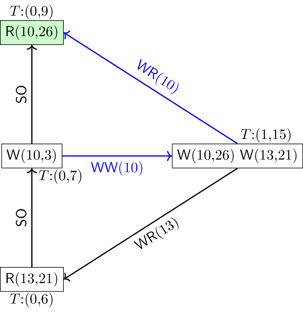
(d) Finalized scenario

Figure 13. Causality violation: the SI anomaly found in YugabyteDB. The recovered dependencies are colored in blue with dashed and solid arrows indicating uncertain and certain dependencies, respectively. The (only) missing transaction is colored in green.

Figure 13 shows how Algorithm 3 interprets a causality violation found in YugabyteDB. MonoSAT reports an undesired cycle $T:(0,7)\xrightarrow{\textsf{WW}(10)}T:(1,15)\xrightarrow{\textsf{WR}(13)}T:(0,6)\xrightarrow{\textsf{SO}}T:(0,7)$; see Figure 13(a). In this scenario, no transactions observe values that have been causally overwritten; consider the only transaction $T:(0,6)$ in Figure 13(a) that reads. To locate the cause of the causality violation, PolySI first finds the (only) “missing” transaction $T:(0,9)$ (colored in green) and the associated dependencies, as shown in Figure 13(b). The WW and RW dependencies are uncertain at this moment (represented by dashed arrows), while the WR dependency is certain (represented by solid arrows, colored in blue). PolySI then restores the violating scenario by resolving such uncertainties. Specifically, as shown in Figure 13(c), PolySI determines that $W(10,3)$ of transaction $T:(0,7)$ was actually installed before $W(10,26)$ of transaction $T:(1,15)$, i.e., $T:(0,7)\xrightarrow{\textsf{WW}(10)}T:(1,15)$. Otherwise, the other direction of dependency $T:(1,15)\xrightarrow{\textsf{WW}(10)}T:(0,7)$ would enforce the dependency $T:(0,9)\xrightarrow{\textsf{RW}(10)}T:(0,7)$, which would create an undesired cycle with the known dependency $T:(0,7)\xrightarrow{\textsf{SO}}T:(0,9)$. Finally, PolySI finalizes the violating scenario by removing the remaining uncertainties from Figure 13(c) to obtain Figure 13(d).

Thanks to the participation of transaction $T:(0,9)$, the cause of the causality violation becomes clear: Transaction $T:(0,7)$ causally depends on transaction $T:(1,15)$, via $T:(1,15)\xrightarrow{\textsf{WR}(13)}T:(0,6)\xrightarrow{\textsf{SO}}T:(0,7)$. However, transaction $T:(0,9)$ following transaction $T:(0,7)$ on the same session reads the value $26$ of key $10$ from transaction $T:(1,15)$, which should have been overwritten by transaction $T:(0,7)$.

Appendix E Minimality of Counterexamples

In this section we show that our interpretation algorithm actually returns a minimal counterexample which contains the cycle found by MonoSAT and is just informative to help understand the violation.

E.1. Definitions

Definition 1.

A violation is a polygraph that fails the checking of PolySI.

Let $C$ be the cycle found by MonoSAT in polygraph $G=\{V,E,Cons\}$. Consider the violation $vio=\{V^{\prime},E^{\prime},Cons^{\prime}\}$ returned by the interpretation algorithm. It satisfies the following properties:

• $vio\subseteq G$, which means $V^{\prime}\subseteq V,E^{\prime}\subseteq E,Cons^{\prime}\subseteq Cons$

• $C\subseteq vio$.

• $vio$ fails the checking of PolySI.

We call $vio$ a violation with respect to $\{G,C\}$.

Definition 2.

A violation $vio$ is minimal, if removing any dependency edge from $vio$ makes it no longer a violation.

There may be more than one minimal violation with respect to $\{G,C\}$. And we name the one who has the least number of dependencies the minimal counter example with respect to $\{G,C\}$, which we expect to get.

Definition 3.

Given a polygraph $G$ and a cycle $C$, there may be more than one minimal violations based on $\{G,C\}$. We name the one which has the least number of dependencies the minimal counterexample with respect to $\{G,C\}$.

E.2. Patterns of Minimal Counterexamples

A minimal counter example is a special polygraph, which consists of several cycles. We define a data structure called ”adjoining cycle set”, and prove that a minimal counterexample is exactly a minimal complete adjoining cycle set.

Definition 4.

A set of cycles $acs$ is called adjoining cycle set, if $\forall$ cycle $C_{1}\in acs$, $\exists$ a constraint $cons=\{dep_{1},.../dep_{2},...\}$ and a cycle $C_{2}\in acs$, s.t. $dep_{1}\in C_{1}$ and $dep_{2}\in C_{2}$.

• $C_{1}$ is the adjoining cycle of $C_{2}$, while $C_{2}$ is the adjoining cycle of $C_{1}$.

• If $\forall$ constraint $cons$, the two choice of $cons$ both have dependencies in $acs$ or neither have dependencies in $acs$, then $acs$ is complete.

Definition 4 describes the data structure called adjoining cycle set. Figure 14 gives an example of adjoining cycle set. When we say a adjoining cycle set is complete, it means no more cycles can be added to the set and each constraint included in the set has two choices. $\{C1,C3\}$ is an adjoining cycle set, but it is incomplete because there exists a constraint (the green one) that has only one choice in $\{C1,C3\}$. $\{C1,C2,C3\}$ is a complete adjoining cycle set, since each constraint has two choices in $\{C1,C2.C3\}$.

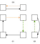
Figure 14. Complete and incomplete adjoining cycle sets. $\{C1,C2,C3\}$ is a complete adjoining cycle set. $\{C1,C2\}$ and $\{C1,C3\}$ are incomplete cycle sets.

Lemma 5.

A minimal violation is exactly a complete adjoining cycle set.

Proof.

If there exists a violation $vio$, which do not contain any complete adjoining cycle set. It contain at least one incomplete cycle set $acs_{1}$, because a violation must have at least one cycle. So there exist a cycle $C_{1}\in acs_{1}$ and a constraint $cons=\{dep_{1}...,/...\}$, where $dep_{1}\in acs_{1}$ and all dependencies in the other choice of $cons$ do not contained by $acs_{1}$. Then we let $cons$ choose the other choice, and then $dep_{1}$ will disappear and $C_{1}$ will not be a cycle any more. Next we focus on $acs_{1}-\{C_{1}\}$, (if $acs_{1}$ has more than one cycle), we will get another incomplete cycle group $acs_{2}=acs_{1}-\{C_{1}\}$. Keep doing this recurisely, all cycles in $acs_{1}$ will be broken. And this polygraph will not be a violation.

If there exists two complete adjoining cycle group in $vio$, then we can delete one complete adjoining cycle group and the left polygraph is still a violation. So it is not a minimal violation.

In conclusion, a minimal violation $vio$ contains exactly one complete adjoining cycle set $acs$. Since both choices of each constraint are in one cycle, $acs$ is a violation that cannot pass the verification of PolySI. $vio$ is a minimal violation, $acs\subseteq vio$ and $acs$ is a violation, then it is trivial that $vio=acs$. ∎

Definition 6.

A complete adjoining cycle set $acs$ is called minimal complete adjoining cycle set containing cycle $C$ if

• $C\in acs$

• $\forall$ complete adjoining cycle set $acs^{\prime}$ containing $C$, the number of dependencies in $acs^{\prime}$ $\geq$ that in $acs$

Theorem 7 (Minimal counterexample).

A minimal complete adjoining cycle set containing cycle $C$ is exactly the minimal counter example with respect to $\{G,C\}$.

Proof.

A minimal complete adjoining cycle set containing $C$ is one of complete adjoining cycle sets containing $C$ which has the least number of dependencies. By lemma 5, it is the smallest minimal violation containing cycle $C$. So it is one of minimal violations with respect to $\{G,C\}$, and has the least number of dependencies. By definition 3, it is exactly the minimal counter example with respect to $\{G,C\}$. ∎

E.3. Restoring Minimal Patterns

The core idea of our interpretation algorithm is to restore the minimal complete adjoining cycle set containing $C$. Function $Find\_ACS$ is designed to do this task. (line 3:19)

For each WW or RW dependency in an undesired cycle, it checks each dependency in the other direction (if missing), and restores the undesired cycles containing these dependencies (line 3:23 - line 3:40). Doing this recursively (line 3:28 and line 3:37), the function will detect all of the adjoining cycle sets that contain $\mathit{Graph_{acs}}$. The minimal one will be returned.

The algorithm uses the brute force and sounds inefficient. However, it works well in practical experiments. From our experience of verification, when it tries to detect a cycle, there usually exists a small cycle with only one WW or RW dependency. For example, in the violation we found in figure 12 a, we first need to find a adjoining cycle from the dependency $T:(9,428)\xrightarrow{}T:{10,471}$. There exists a simple cycle $T:(10,471)\xrightarrow{}T:(4,172)\xrightarrow{}T:(10,467)\xrightarrow{}T:(10,471)$. This cycle has a small size and only has one WW dependency, which means the function does not need to detect more cycles recursively in order to restore a complete adjoining cycle set, and can pay no attention to other possible adjoining cycle sets that contain more than 3 dependencies.

However, there still exist the worst cases that the interpretation algorithm cannot return the minimal counter example quickly. But in this case, we can be more patient to wait for it. Since we have already known the result that there exists a violation, and we just need to wait for the minimal counter example. And if it still costs too much time, we can interrupt it and output a minimal violation we have found instead of the smallest one, after the interpretation algorithm has run enough time.

Theorem 8 (Minimality).

PolySI always returns a minimal counterexample with respect to $G$ and $C$, with $G$ the polygraph built from a history and $C$ the cycle output by MonoSAT.

Proof.

Our interpretation algorithm will return a ‘minimal complete adjoining cycle set’ containing cycle $C$, which is exactly the minimal counter example. ∎

Now we have restored the minimal counter example. However, to help understand the violation, we still restore some more dependencies. For each $rw$ dependency appears in violations, it is caused by a $wr$ dependency and a $ww$ dependency. If we delete the $wr$ dependency and $ww$ dependency, it is difficult to understand the $rw$ dependency. So for each $rw$ dependency in a minimal counterexample, we recover the related $wr$ and $ww$ dependencies to the violation (Alg3:line13-16). This is very useful in our experiments. For example, in the violation we found in figure 5, the transaction $T:(1,4)$ is recovered from two $rw$ dependencies. Without the recovered transaction, it is difficult to understand the violation.

Appendix F Performance Evaluation of PolySI-List

Figure 15 shows the performance evaluation of PolySI-List, the extension to PolySI for handling Elle-like logs/histories with the “list” data structure.

0.23    0.23

0.23    0.23

0.23    0.23

Figure 15. Performance evaluation of PolySI-List.

References

- (1)
- Adya (1999) Atul Adya. 1999. Weak Consistency: A Generalized Theory and Optimistic Implementations for Distributed Transactions. Ph.D. Dissertation. USA.
- Bailis et al. (2013) Peter Bailis, Aaron Davidson, Alan Fekete, Ali Ghodsi, Joseph M. Hellerstein, and Ion Stoica. 2013. Highly Available Transactions: Virtues and Limitations. Proc. VLDB Endow. 7, 3 (nov 2013), 181–192. https://doi.org/10.14778/2732232.2732237
- Bailis et al. (2016) Peter Bailis, Alan Fekete, Ali Ghodsi, Joseph M. Hellerstein, and Ion Stoica. 2016. Scalable Atomic Visibility with RAMP Transactions. ACM Trans. Database Syst. 41, 3, Article 15 (jul 2016), 45 pages. https://doi.org/10.1145/2909870
- Bayless et al. (2015) Sam Bayless, Noah Bayless, Holger H. Hoos, and Alan J. Hu. 2015. SAT modulo Monotonic Theories. In Proceedings of the Twenty-Ninth AAAI Conference on Artificial Intelligence (AAAI’15). AAAI Press, 3702–3709.
- Berenson et al. (1995) Hal Berenson, Phil Bernstein, Jim Gray, Jim Melton, Elizabeth O’Neil, and Patrick O’Neil. 1995. A Critique of ANSI SQL Isolation Levels. In SIGMOD ’95. ACM, 1–10. https://doi.org/10.1145/223784.223785
- Bernstein et al. (1986) Philip A Bernstein, Vassos Hadzilacos, and Nathan Goodman. 1986. Concurrency Control and Recovery in Database Systems. Addison-Wesley Longman Publishing Co., Inc., USA.
- Biswas and Enea (2019) Ranadeep Biswas and Constantin Enea. 2019. On the Complexity of Checking Transactional Consistency. Proc. ACM Program. Lang. 3, OOPSLA, Article 165 (Oct. 2019), 28 pages. https://doi.org/10.1145/3360591
- Biswas et al. (2021) Ranadeep Biswas, Diptanshu Kakwani, Jyothi Vedurada, Constantin Enea, and Akash Lal. 2021. MonkeyDB: Effectively Testing Correctness under Weak Isolation Levels. Proc. ACM Program. Lang. 5, OOPSLA, Article 132 (oct 2021), 27 pages. https://doi.org/10.1145/3485546
- Bouajjani et al. (2017) Ahmed Bouajjani, Constantin Enea, Rachid Guerraoui, and Jad Hamza. 2017. On verifying causal consistency. In POPL’17. ACM, 626–638.
- Cerone et al. (2015) Andrea Cerone, Giovanni Bernardi, and Alexey Gotsman. 2015. A Framework for Transactional Consistency Models with Atomic Visibility. In CONCUR’15 (LIPIcs), Vol. 42. Schloss Dagstuhl–Leibniz-Zentrum fuer Informatik, 58–71.
- Cerone and Gotsman (2018) Andrea Cerone and Alexey Gotsman. 2018. Analysing Snapshot Isolation. J. ACM 65, 2, Article 11 (Jan. 2018), 41 pages. https://doi.org/10.1145/3152396
- Chen et al. (2020) Haicheng Chen, Wensheng Dou, Dong Wang, and Feng Qin. 2020. CoFI: Consistency-Guided Fault Injection for Cloud Systems. In ASE 2020. IEEE. https://doi.org/10.1145/3324884.3416548
- Clavel et al. (2007) Manuel Clavel, Francisco Durán, Steven Eker, Patrick Lincoln, Narciso Martí-Oliet, José Meseguer, and Carolyn Talcott. 2007. All about Maude - a High-Performance Logical Framework: How to Specify, Program and Verify Systems in Rewriting Logic. Springer-Verlag, Berlin, Heidelberg.
- Cluster (2022) MariaDB Galera Cluster. Accessed August, 2022. https://mariadb.com/kb/en/what-is-mariadb-galera-cluster/.
- CockroachDB (2022) CockroachDB. Accessed August, 2022. https://www.cockroachlabs.com/.
- Cormen et al. (2009) Thomas H. Cormen, Charles E. Leiserson, Ronald L. Rivest, and Clifford Stein. 2009. Introduction to Algorithms, Third Edition (3rd ed.). The MIT Press.
- Crooks et al. (2017) Natacha Crooks, Youer Pu, Lorenzo Alvisi, and Allen Clement. 2017. Seeing is Believing: A Client-Centric Specification of Database Isolation. In PODC ’17. ACM, 73–82. https://doi.org/10.1145/3087801.3087802
- Darnell (2022) Ben Darnell. Accessed August, 2022. Lessons Learned from 2+ Years of Nightly Jepsen Tests. https://www.cockroachlabs.com/blog/jepsen-tests-lessons/.
- Database (2022) Oracle Database. Accessed August, 2022. https://www.oracle.com/database/.
- Daudjee and Salem (2006) Khuzaima Daudjee and Kenneth Salem. 2006. Lazy Database Replication with Snapshot Isolation. In VLDB’06. VLDB Endowment, 715–726.
- Dgraph (2022) Dgraph. Accessed August, 2022. https://dgraph.io/.
- Didona et al. (2018) Diego Didona, Rachid Guerraoui, Jingjing Wang, and Willy Zwaenepoel. 2018. Causal Consistency and Latency Optimality: Friend or Foe? Proc. VLDB Endow. 11, 11 (2018), 1618–1632.
- Gan et al. (2020) Yifan Gan, Xueyuan Ren, Drew Ripberger, Spyros Blanas, and Yang Wang. 2020. IsoDiff: Debugging Anomalies Caused by Weak Isolation. Proc. VLDB Endow. 13, 12 (July 2020), 2773–2786. https://doi.org/10.14778/3407790.3407860
- Graphviz (2022) Graphviz. Accessed December, 2022. Open source graph visualization software. https://graphviz.org/.
- Helt et al. (2021) Jeffrey Helt, Matthew Burke, Amit Levy, and Wyatt Lloyd. 2021. Regular Sequential Serializability and Regular Sequential Consistency. In SOSP’21. ACM, 163–179.
- Huang et al. (2023) Kaile Huang, Si Liu, Zhenge Chen, Hengfeng Wei, David Basin, Haixiang Li, and Anqun Pan. 2023. Efficient Black-Box Checking of Snapshot Isolation in Databases. Proc. VLDB Endow. 16, 6 (apr 2023), 1264–1276. https://doi.org/10.14778/3583140.3583145
- Huang et al. (2022) Kaile Huang, Si Liu, Zhenge Chen, Hengfeng Wei, David Basin, Haixiang Li, and Anqun Pan. Accessed December, 2022. Issue #17. https://github.com/jepsen-io/elle/issues/17.
- Jepsen (2022a) Jepsen. Accessed August, 2022a. https://jepsen.io.
- Jepsen (2022b) Jepsen. Accessed August, 2022b. Issue #824. https://github.com/YugaByte/yugabyte-db/issues/824.
- Kallen (2022) Nick Kallen. Accessed August, 2022. Big Data in Real Time at Twitter. https://www.infoq.com/presentations/Big-Data-in-Real-Time-at-Twitter/.
- Kingsbury and Alvaro (2020) Kyle Kingsbury and Peter Alvaro. 2020. Elle: Inferring Isolation Anomalies from Experimental Observations. Proc. VLDB Endow. 14, 3 (Nov. 2020), 268–280.
- Lamport (1978) Leslie Lamport. 1978. Time, Clocks, and the Ordering of Events in a Distributed System. Commun. ACM 21, 7 (1978), 558–565.
- Liu et al. (2019) Si Liu, Peter Csaba Ölveczky, Min Zhang, Qi Wang, and José Meseguer. 2019. Automatic Analysis of Consistency Properties of Distributed Transaction Systems in Maude. In TACAS 2019 (LNCS), Vol. 11428. Springer, 40–57.
- Lloyd et al. (2013) Wyatt Lloyd, Michael J. Freedman, Michael Kaminsky, and David G. Andersen. 2013. Stronger semantics for low-latency geo-replicated storage. In NSDI’ 13. USENIX Association, 313–328.
- Lu et al. (2020) Haonan Lu, Siddhartha Sen, and Wyatt Lloyd. 2020. Performance-Optimal Read-Only Transactions. In OSDI 2020. USENIX Association, 333–349.
- MongoDB (2022) MongoDB. Accessed August, 2022. https://www.mongodb.com/.
- Papadimitriou (1979) Christos H. Papadimitriou. 1979. The Serializability of Concurrent Database Updates. J. ACM 26, 4 (oct 1979), 631–653. https://doi.org/10.1145/322154.322158
- Peng and Dabek (2010) Daniel Peng and Frank Dabek. 2010. Large-Scale Incremental Processing Using Distributed Transactions and Notifications. In OSDI’10. USENIX Association, USA, 251–264.
- PostgreSQL (2022) PostgreSQL. Accessed August, 2022. Transaction Isolation. https://www.postgresql.org/docs/current/transaction-iso.html.
- RUBiS (2022) RUBiS. Accessed August, 2022. Auction Site for e-Commerce Technologies Benchmarking. https://projects.ow2.org/view/rubis/.
- Server (2022) Microsoft SQL Server. Accessed August, 2022. https://www.microsoft.com/en-us/sql-server/.
- Shang et al. (2018) Zechao Shang, Jeffrey Xu Yu, and Aaron J. Elmore. 2018. RushMon: Real-Time Isolation Anomalies Monitoring. In SIGMOD ’18. ACM, 647–662. https://doi.org/10.1145/3183713.3196932
- Sovran et al. (2011) Yair Sovran, Russell Power, Marcos K. Aguilera, and Jinyang Li. 2011. Transactional Storage for Geo-Replicated Systems. In SOSP ’11. ACM, 385–400. https://doi.org/10.1145/2043556.2043592
- Tan et al. (2020) Cheng Tan, Changgeng Zhao, Shuai Mu, and Michael Walfish. 2020. COBRA: Making Transactional Key-Value Stores Verifiably Serializable. In OSDI’20. Article 4, 18 pages.
- Terry et al. (1994) Douglas B. Terry, Alan J. Demers, Karin Petersen, Mike Spreitzer, Marvin Theimer, and Brent B. Welch. 1994. Session Guarantees for Weakly Consistent Replicated Data. In PDIS. IEEE Computer Society, 140–149.
- testing of MongoDB 4.2.6 (2022) Jepsen testing of MongoDB 4.2.6. Accessed August, 2022. http://jepsen.io/analyses/mongodb-4.2.6.
- testing of TiDB 2.1.7 (2022) Jepsen testing of TiDB 2.1.7. Accessed August, 2022. https://jepsen.io/analyses/tidb-2.1.7.
- TiDB (2022) TiDB. Accessed August, 2022. https://en.pingcap.com/tidb/.
- TPC (2022) TPC. Accessed August, 2022. TPC-C: On-Line Transaction Processing Benchmark. https://www.tpc.org/tpcc/.
- Warszawski and Bailis (2017) Todd Warszawski and Peter Bailis. 2017. ACIDRain: Concurrency-Related Attacks on Database-Backed Web Applications. In SIGMOD 2017. ACM, 5–20. https://doi.org/10.1145/3035918.3064037
- Xiong et al. (2020) Shale Xiong, Andrea Cerone, Azalea Raad, and Philippa Gardner. 2020. Data Consistency in Transactional Storage Systems: A Centralised Semantics. In ECOOP’20, Vol. 166. 21:1–21:31. https://doi.org/10.4230/LIPIcs.ECOOP.2020.21
- YugabyteDB (2022) YugabyteDB. Accessed August, 2022. https://www.yugabyte.com/.
- Zellag and Kemme (2014) Kamal Zellag and Bettina Kemme. 2014. Consistency anomalies in multi-tier architectures: automatic detection and prevention. VLDB J. 23, 1 (2014), 147–172. https://doi.org/10.1007/s00778-013-0318-x
- Zennou et al. (2019) Rachid Zennou, Ranadeep Biswas, Ahmed Bouajjani, Constantin Enea, and Mohammed Erradi. 2019. Checking Causal Consistency of Distributed Databases. In NETYS 2019 (LNCS), Vol. 11704. Springer, 35–51. https://doi.org/10.1007/978-3-030-31277-0_3