Multi-compartment Neuron and Population Encoding improved Spiking Neural Network for Deep Distributional Reinforcement Learning

SUMMARY

Inspired by the information processing with binary spikes in the brain, the spiking neural networks (SNNs) exhibit significant low energy consumption and are more suitable for incorporating multi-scale biological characteristics. Spiking Neurons, as the basic information processing unit of SNNs, are often simplified in most SNNs which only consider LIF point neuron and do not take into account the multi-compartmental structural properties of biological neurons. This limits the computational and learning capabilities of SNNs. In this paper, we proposed a brain-inspired SNN-based deep distributional reinforcement learning algorithm with combination of bio-inspired multi-compartment neuron (MCN) model and population coding method. The proposed multi-compartment neuron built the structure and function of apical dendritic, basal dendritic, and somatic computing compartments to achieve the computational power close to that of biological neurons. Besides, we present an implicit fractional embedding method based on spiking neuron population encoding. We tested our model on Atari games, and the experiment results show that the performance of our model surpasses the vanilla ANN-based FQF model and ANN-SNN conversion method based Spiking-FQF models. The ablation experiments show that the proposed multi-compartment neural model and quantile fraction implicit population spike representation play an important role in realizing SNN-based deep distributional reinforcement learning.

INTRODUCTION

Spiking neural networks building the biological neuron dynamic model have advantages of energy efficiency and robustness. Recently, neuromorphic computing has successfully applied SNNs to various fields such as image classification Vaila [2021], Lee et al. [2020], Li and Zeng [2022], object detection Kim et al. [2020], Luo et al. [2021], speech recognition Dominguez-Morales et al. [2018], Ponghiran and Roy [2022], decision making Tan et al. [2021], Zhao et al. [2018], Sun et al. [2022] and robot control Balachandar and Michmizos [2020], Tang et al. [2020a]. SNNs achieves comparable performance to traditional ANNs, and the neuromorphic hardware enables SNN deploying and training with low power consumption and biological plausibility Merolla et al. [2014], Furber et al. [2014], Davies et al. [2018].

Different from conventional artificial neuron models, like Sigmoids and ReLU, the spiking neuron in SNNs process the input signal to the dynamical membrane potential. When the potential exceeds the threshold, it fires a spike as output. Although the dynamic details of spiking neuron models increase the computing capability of the network, they rarely take advantage of the structural properties of biological neurons. Moreover the role of computing power in different parts of neurons on complex tasks still needs further exploration. The Leaky Integrate-and-Fire (LIF) Gerstner and Kistler [2002] model takes neurons as point-like structures similar to the traditional artificial neuron model, which only uses the somatic membrane potential to process the input signal. Some other spiking neuron models, such as the Izhikevich neuron Izhikevich [2004] and Hodgkin-Huxley neuron Hodgkin et al. [1952], have more dynamic characteristics than the LIF model but still do not consider the neurons’ structure characteristics.

Neurobiological research has found that neuron dendrites have a unique role in integrating synaptic inputs, which can increase the information processing capacity of neurons Kampa and Stuart [2006], Smith et al. [2013], Gidon et al. [2020]. The neurons in the mammalian forebrain have relatively separate computing compartments, and a two-layer neural network model is needed to predict the cell’s firing rate for complex stimuli Poirazi et al. [2003]. The dendritic prediction method provides a two-compartment neuron model consisting of soma and dendrite modules. It optimizes the dendritic synapse weights to minimize the inconsistency between the dendritic potential and somatic firing rate Urbanczik and Senn [2014], Sacramento et al. [2018]. The three-compartment model of neocortical neurons consists of apical dendrites, basal dendrites, and soma. The multi-layer network of these segregated compartments neurons is used to classify the MNIST images Richards et al. [2019]. The target-based learning uses the apical dendrite to receive the plasticity signal, and neurons’ weights can be modified locally Lansdell et al. [2019], Capone et al. [2022]. Besides, the multi-compartment neuron models implemented on neuromorphic chips can simulate the dynamic processes of the brain’s neural circuits with extremely low power consumption Shrestha et al. [2021], Kopsick et al. [2022].

Although the multi-compartment neuron (MCN) model has been studied on many tasks, they are all focus on processing information with simple features like MNIST images and neuron spiking sequence. There is still a lack of exploration on complex decision-making tasks (such as playing computer video games) based on multi-compartment SNNs. In this work, we take inspiration from the structure of pyramidal neurons in the human cortex and propose a multi-compartment neuron model comprising apical dendrite, basal dendrite, and soma computing compartments. Different with the multi-compartment neuron model processing single source information as mentioned above, we use the the apical and basal dendrites receive decision-making signals from different sources, and the somatic potential integrate the input information of the two compartments which generates spikes output when the somatic potential exceeds the threshold Polsky et al. [2004], Makara and Magee [2013]. We introduce the multi-compartment neuron into deep distributional reinforcement learning and implement a multi-compartment spiking FQF Yang et al. [2019] model.

The population encoding plays a vital role in the brain to precisely represent continuous real-valued values and achieve robustness in functional information processing Sanger [2003], Panzeri et al. [2015]. And the dynamic population encoding helps the brain better deal with working memory tasks Meyers [2018]. Inspired by the population neural encoding mechanism in brain, we propose a spiking quantile fraction value population encoding method, which represent the quantile fraction in spike information space and further input the population spikes to the apical dendrite of MCN neuron as one of decision-making source signals.

Recently, several works use SNNs to solve reinforcement learning (RL) problems, implementing a range of work such as Spiking DQN. For further applying SNNs (with efficient binary spikes) to continuous control tasks, the PopSAN model builds a population-coded spiking actor network and is hybrid trained with a deep critic network Tang et al. [2020b, a]. SNNs are inherently challenging to be optimized, and the dynamical learning environment makes it difficult to train the SNNs directly to realize deep reinforcement learning (DRL). Tan et al. [2021] achieves comparable performance on Atari games through converting DQN to SNN. In addition, the SNNs are inherently challenging to be optimized and need more stable supervision information than ANNs. The knowledge distillation is used to train SNNs in DRL with a DQN teacher and an SNN student Zhang et al. [2021]. With the surrogate function to approximate the spike gradient, the gradient-based optimization method, Spatio-temporal Backpropagation (STBP), is used to train the Spikng-DQN model directly Liu et al. [2021], Chen et al. [2022]. The PL-SDQN Sun et al. [2022] solves the spiking vanish problem in the deep spiking convolutional layer of SNNs in DRL with a potential-based layer normalization method. However, existing works only build simple deep SNN structure like the network in vanilla DQN, which would be a great challenge for supporting more complex decision-making tasks, such as distributional reinforcement learning. In addition, more effective and biologically plausible SNN models need to be developed in order to overcome the difficulty of training SNNs, and the limitation in integrating information from point neurons.

This work introduces SNNs to the field of deep distributional reinforcement reinforcement learning for the first time, and proposes a novel MCS-FQF model that combines biologically plausible multi-compartment neuron model with a precise population encoding strategy.

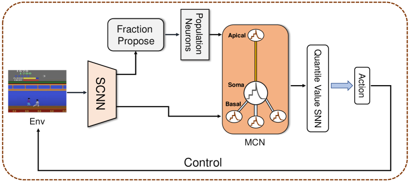
Figure S1: The overall architecture of MCS-FQF model.

We propose the multi-compartment spiking fully parameterized quantile function network (MCS-FQF) model and firstly applies SNN to the field of deep distributional reinforcement learning. Distributional reinforcement learning estimates the value distribution as returns and is more similar to the decision-making process in the human brain  Lowet et al. [2020]. Figure S1 in Supplementary Material depicts the overall architecture of our proposed MCS-FQF model, we first use a spiking convolutional network (SCNN) to embed game video observation states to spike trains and then implement a spiking neuron population encoding method to generate the implicit spiking representations of quantile fraction from the spiking state embedding. The multi-compartment neuron model integrates the state and quantile fraction information. The basal dendrite module receives the state embedding spike inputs, and the apical dendrites module processes the spiking population embedding of quantile fraction . The information in the basal and apical dendritic potentials is integrated at the somatic module. The firing outputs of the multi-compartment neuron are used as spike representations combining state and quantile fraction. Finally, a fully connected SNN processes the spike outputs of the multi-compartment neuron to generate quantile values. The other multi-compartment neural networks are relatively shallow and the training method can not been extending to deep structures in different tasks. Instead, we propose the directly training algorithm of MCN model. We use the surrogate function to approximate the MCN’s spike gradient and derive STBP method for MCN weight optimization. By training the MCS-FQF model with end-to-end gradient descent algorithm, the MCF-FQF model achieve significant performance on Atari environment.

We summarize the main contribution of this paper as follow:

• We present a brain-inspired MCS-FQF model to explores the application of SNNs on complex distributional reinforcement learning tasks.

• We provide a thorough analysis on various the functions of different structure compartment of biological neurons and build the multi-compartment neuron model to extend the computing capability of a single spiking neuron.

• The proposed MCS-FQF model takes into account a biologically plausible population encoding method that enables the spiking neural networks to precisely represent the continuous fraction values. And the experiment shows the brain-inspired population encoding method is more efficient than cosine embedding in traditional FQF model for representing the selective scalar fraction values in spiking neural networks.

• Extensive experiments demonstrate that the proposed MCS-FQF model achieves better performance than the vanilla FQF model and ANN-SNN conversion based Spiking-FQF model on Atari game experiments. Moreover, the ablation study results show that the population encoding and MCN model has irreplaceable contributions in boosting the capability of spike neurons in information representation and integration.

Methods

Multi-compartment Neuron Model for Information Integration

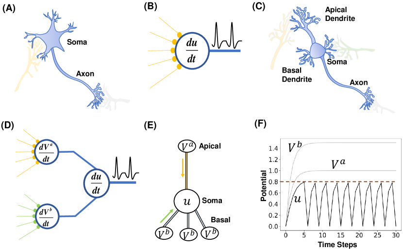
Figure 1: Point neuron model and multi-compartment neuron model. (A) Point neuron with soma compartment. (B) Computational model for point neuron with single information processing node. (C) Multi-compartment neuron with basal dendrite, apical dendrite and soma. (D) Computational model for multi-compartment neuron. (E)Structure and potentials influence of MCN. (F) Firing activity of MCN model. The potentials are recorded from constant inputs signal with $x_{a}=1.0$ and $x_{b}=1.5$ within $T=30$ time steps. The parameters of MCN model are set as $\tau_{A}=\tau_{B}=2.0$, $\tau_{L}=4.0$, $g_{A}=g_{B}=g_{L}=1.0$, and the threshold potential is $V_{th}=0.8$.

The LIF neuron is a point structures computing model described by Eq. (1). It only uses the somatic membrane potential $u_{t}$ to process the input signal $x_{t}$. When $u_{t}$ exceeds the threshold $V_{th}$, the neuron fires a spike as $s_{t}=1$, otherwise $s_{t}=0$ for no spikes.

$$\left\{\begin{array}[]{l}\tau_{L}\frac{du_{t}}{dt}=-u_{t}+x_{t},\\ s_{t}=1,u_{t}\leftarrow V_{reset}\quad\text{if}\ u_{t}>V_{th}.\end{array}\right.$$ (1)

Inspired by the dendritic integration function of pyramidal neurons in hippocampal CA3 Makara and Magee [2013], we build a multi-compartment neuron model to fuse the state and quantile fraction information. Unlike the LIF neuron model, the MCN model has three compartments, including basal dendrite, apical dendrite, and soma, as shown in Figure 1. The basal and apical dendrite modules have weighted synapses and receive information from different input sources. The apical dendrites are farther from the soma and receive modulated signals from other regions. The basal dendrites surround the soma and receive feedforward inputs.

$$\left\{\begin{array}[]{l}\tau_{B}\frac{dV_{t}^{b}}{dt}=-V_{t}^{b}+x_{t}^{b}\\ x_{t}^{b}=\sum_{j}w^{b}_{j}o^{b}_{j,t}\end{array}\right.$$ (2)

The computing process of the basal dendrite is described by Eq. 2. The $o^{b}_{j,t}$ is the spike signal neuron $j$ input to the basal dendrite at time step $t$. It is summed by the weighted synapse $w_{b}$ to the dendritic postsynaptic potential $x^{b}_{t}$. The dendritic potential $V^{b}_{t}$ integrates $x^{b}_{t}$ with time constant $\tau_{B}$.

$$\left\{\begin{array}[]{l}\tau_{A}\frac{dV^{a}_{t}}{dt}=-V^{a}_{t}+x^{a}_{t}\\ x^{a}_{t}=\sum_{j}w^{a}_{j}o^{a}_{j,t}\end{array}\right.$$ (3)

In our proposed MCN model, the apical dendrites have the same computational form as basal dendrites. The apical dendrite computing process is shown in Eq. (3). Although apical dendrites may have more unique abilities, we prefer focusing on the neuron’s ability to integrate disparate information in this work and use the MCN model to process the embedding spike signals of state and quantile fraction. The basal and apical dendrite synaptic weights are learnable parameters, making MCN an adaptable node for information integration.

The potentials of basal and apical dendrites are conducted to the soma compartment, and the MCN model integrates this information to the somatic potential $u_{t}$ as in Eq. (4).

$$\tau_{L}\frac{du_{t}}{dt}=-u_{t}+\frac{g_{B}}{g_{L}}(V^{b}_{t}-u_{t})+\frac{g_{A}}{g_{L}}(V^{a}_{t}-u_{t})$$ (4)

where the $g_{B}$, $g_{A}$ and $g_{L}$ are constant hyperparameters as basal dendrite conductance, apical dendrite conductance, and leaky conductance, respectively, the $\tau_{L}$ is the somatic leaky time constant. The neuron fires a spike when the somatic potential $u_{t}$ exceeds the threshold $V_{th}$. We omit the time step subscripts below for brevity.

Theorem 1

Let $Z=\frac{g_{B}+g_{A}+g_{L}}{\tau_{L}g_{L}}$, the somatic potential $u(t)$ is the spatial-temporal integration of the apical and basal dendritic potentials as:

$$u(t)=\int^{t}_{-\infty}\frac{e^{Zt}}{\tau_{L}}[\frac{g_{B}}{g_{L}}V^{b}(t)+\frac{g_{A}}{g_{L}}V^{a}(t)]dte^{-Zt}.$$ (5)

The proof of Theorem 5 can been seen in the supplementary materials. Compared with point neuron models, which combine input signals with the simple sum operation, the MCN model integrates apical and basal dendritic potentials at spatial-temporal dimensions as in Eq. (5). The relationship between MCN somatic and dendritic potentials is shown in Figure 1(E)(F).

Population Encoding For Quantile Fraction Implicit Representation

Quantile regression based distributional reinforcement learning needs the models take the selected quantile fractions $\tau$ as inputs and output the corresponding quantile values. The quantile fraction is proposed by a fully parameterized function with the value’s range is $\tau\in[0,1]$. To combine SNN with deep distributional reinforcement learning, we propose a population encoding method to use the neural spikes as the implicit representation of quantile fraction. We use $M$ neurons with stimulus selective sensitivity as the encoding neuron populations. Each neuron has a Gaussian receptive field, and the relationship between the $j_{th}$ neuron’s spike firing rate $r_{j}$ and its input stimulus $s_{j}$ is

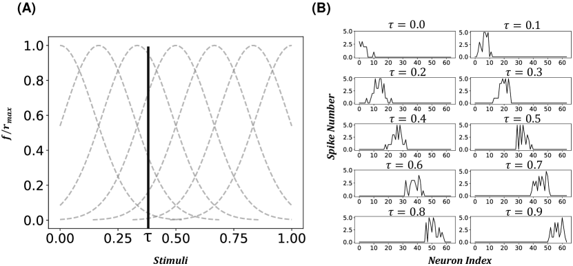
Figure 2: The spiking activity of population neuron. (A) Population neurons with Gaussian receptive field. The gray dotted line represents the relationship between the firing rate of different neurons and input stimuli. The intersection of the solid vertical line with the activity curve of each neuron is the firing rate of that neuron when encoding the corresponding quantile fraction value. (B) The spike numbers of $M=64$ neurons within $T=8$ time periods when representing different fraction values.

$$r_{j}=\phi_{j}exp(-\frac{(s_{j}-\mu_{j})^{2}}{2\sigma^{2}_{j}})$$ (6)

where $\mu_{j}$ is the input stimulus which is most consistent with the neuron’s expectations and is also the largest firing rate point. And the $\sigma_{j}$ determines the range of the receptive field; the smaller the value of $\sigma_{j}$, the more selective the neuron is for the input stimulus, as shown in Figure 2(A).

To represent the quantile fractions with population neural spikes, we encode the $i_{th}$ fraction value $\tau_{i}$ to the collaborative activities of the $M$ neurons. The firing rate of the $j_{th}$ neuron for the value $\tau_{i}$ is

$$r_{ij}=\phi_{j}exp(-\frac{(\tau_{i}-\mu_{j})^{2}}{2\sigma^{2}_{j}})$$ (7)

and each neuron has a unique preferred stimulus with $\mu_{i}=\frac{i}{N}$. Because the quantile fractions are homogeneous values ranging from 0 to 1, all neurons have same receptive characteristic as

$$\forall i\in[1,2,..,M],\sigma_{i}=C$$ (8)

The neurons’ spiking activity is a Poisson process. And the quantile fraction $\tau_{i}$ is encoded to population spike $S_{\tau_{i}}$ as Eq.(10). The neuron $j$ fires $n$ spikes within time interval $\Delta t$ with possibility $P_{ij,\Delta t}[n]$.

$$S_{\tau_{i,j}}\sim P_{ij,\Delta t}[n]=\frac{(r_{ij}\Delta t)^{2}}{n!}exp(-r_{ij}\Delta t)$$ (9)

$$S_{\tau_{i}}=\{S_{\tau_{i,j}},j=\{1,2,...,M\}\}$$ (10)

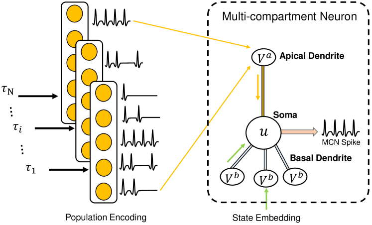
Figure S2: Encoding quantile fraction value with population neuron.

We use $M=64$ neurons to encode fraction values. Figure 2(B) depicts the firing activity of population neurons when encoding different fraction values. The spiking implicit representation of fraction value is input to the apical dendrite, and the apical dendritic potential $V^{a}$ is then integrated with observation state information in soma of multi-compartment neuron as shown in Figure S2.

Multi-compartment Spiking-FQF Model

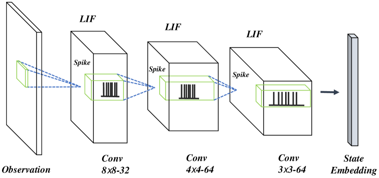
Figure S3: Spiking convolutional neural network used for encoding image observation to spike state embedding. The note ”8x8-32” means that the convolution layer has the structure of ”8x8” kernel size and 32 feature channels.

We propose MCS-FQF model based on the multi-compartment neuron and population encoding method, as shown in Figure 3, which is the first work that applies SNNs to deep distributional reinforcement learning as far as we know. The MCS-FQF model implements a spiking convolution neural network (SCNN) to extract state embedding spike trains from the games video observation as shown in Figure S3. The SCNN is built with LIF neurons and consists of three convolution layers and the spike embedding of state $O^{s}$ is generated from the outputs of SCNN.

We set the number of quantile fractions to $N$ with $\tau_{0}=0$, $\tau_{N}=1$, and for $i=[1,...,N-1]$, $\tau_{i-1}<\tau_{i}$ as in Yang et al. [2019]. And we calculate the quantile fraction with cumulative distribution probability generated from $O^{s}$ as Eq. (11-13). The state embedding is processed by learnable weight $W^{f}$, and the mean activities of SCNN neuron within $T$ time window are regarded as logits of quantile fraction probability.

$$\phi_{i}=\frac{1}{T}\sum_{t=0}^{T-1}W^{f}_{i}O^{s}_{t}$$ (11)

$$p_{k}=\frac{exp(\phi_{k})}{\sum_{j}exp(\phi_{j})}$$ (12)

$$\tau_{i}=\sum_{k=0}^{i-1}p_{k}$$ (13)

Multi-compartment neurons integrate the state and quantile fraction embeddings as Eq. (14-16). The apical dendrite receives the fraction representation spikes, and the basal dendrite receives the state embedding inputs. The somatic potential $u$ is the confluence of the basal dendritic potential $V_{s}^{b}$ and the apical dendritic potential $V_{\tau}^{a}$.

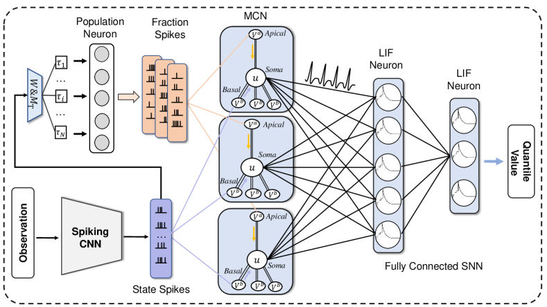
Figure 3: The framework of MCS-FQF. Multi-compartment neurons receive the state embedding inputs from spiking convolution neural network and the quantile fraction encoding inputs from population neurons. The somatic spikes of MCN input to a fully connected SNN to generate the quantile value.

$$\left\{\begin{array}[]{l}\tau_{B}\frac{dV_{s}^{b}}{dt}=-V_{s}^{b}+x^{b}\\ x^{b}=\sum_{j}w^{b}_{j}O^{s}_{j}\end{array}\right.$$ (14)

$$\left\{\begin{array}[]{l}\tau_{A}\frac{dV_{\tau}^{a}}{dt}=-V_{\tau}^{a}+x^{a}\\ x^{a}=\sum_{j}w^{a}_{j}S_{\tau,j}\end{array}\right.$$ (15)

$$\tau_{L}\frac{du}{dt}=-u+\frac{g_{B}}{g_{L}}(V_{s}^{b}-u)+\frac{g_{A}}{g_{L}}(V_{\tau}^{a}-u)$$ (16)

The MCN fires spike trains $S^{m}(t)$ when the potential $u_{t}$ exceeds the threshold potential $V_{th}$. The final two-layer fully connected LIF neuron SNN processes the MCN’s spikes, and the quantile values $F^{-1}_{w}(\tau_{i})$ are estimated from the output spikes of the final SNN as Eq. (17). The weight parameter $W^{L}$ is optimized with the whole network. The complete MCS-FQF calculating process is shown in Algorithm 1. The MCS-FQF model generates state-action value as Eq. (18).

Algorithm 1 Proceeding process of MCS-FQF

Input: Observation state $S_{t}$
Parameter: Decay factor $\tau_{L}$, $\tau_{A}$, $\tau_{B}$; conductance $g_{A}$, $g_{B}$, $g_{L}$; fraction number $N$, population number $M$; simulation time-window $T$; membrane potential threshold $V_{th}$; layers number $L$.
Output: State-action values $Q$.

1:  Initialize neuron weight $w^{l}$ and potential $u^{l}_{0}$ $\forall\ l=0,1,2,...,L-1$.

2:  // Compute the state embedding

3:  for $t=0$ to $T-1$ do

4:     $O^{s}_{t}=SCNN(S_{t})$

5:  end for

6:  // Compute the fractions

7:  for $i=1$ to $N$ do

8:     for $t=0$ to $T-1$ do

9:        $\tau_{i}=F(W^{f}O^{s}_{t})$ as in Eq. (10)-(12)

10:     end for

11:  end for

12:  // Compute the quantile values $F^{-1}_{w}$

13:  for $t=0$ to $T-1$ do

14:      // Calculate fraction embedding by population

15:      // encoding

16:     for $j=0$ to $M-1$ do

17:        $S_{\tau_{j},t}=LIF(PopEmb(\tau_{j}))$

18:     end for

19:     for $i=0$ to $N-1$ do

20:        $F^{-1}_{w}(\tau_{i},t)=SNN(MCN(S_{\tau_{j},t},O^{s}_{t}))$

21:     end for

22:  end for

23:  Calculate state-action value $Q$ as Eq. (17).

24:  return $Q$

$$F^{-1}_{w}(\tau_{i})=\frac{1}{T}\sum_{t=0}^{T-1}W^{L}O^{L}_{i,t}$$ (17)

$$Q(s,a)=\sum_{i=0}^{N-1}(\tau_{i+1}-\tau_{i})F^{-1}_{w}(\hat{\tau}_{i})$$ (18)

$$\hat{\tau}_{i}=\frac{\tau_{i}+\tau_{i+1}}{2}$$ (19)

We train the MCS-FQF model by using STBP algorithm Wu et al. [2018]. The weights of SCNN and the final fully connected SNN are optimized by minimizing the Huber quantile regression loss Huber [1992] $\mathbb{HL}(*)$:

$$\mathbb{HL}(\tau,\delta_{ij})=|\tau-(1-\mathbb{H}(\delta_{ij}))|\frac{\mathbb{L}(\epsilon,\delta_{i,j})}{\epsilon}$$ (20)

$$\mathbb{L}(\epsilon,\delta_{i,j})=\left\{\begin{array}[]{ll}\frac{1}{2}\delta^{2}_{ij},&\text{if}~{}|\delta_{ij}|\leq\epsilon\\ \epsilon(|\delta_{ij}|-\frac{1}{2}\epsilon)&\text{otherwise}.\end{array}\right.$$ (21)

$$\mathbb{H}(\delta_{ij})=\left\{\begin{array}[]{ll}0,&\text{if}~{}\delta_{ij}\leq 0\\ 1,&\text{otherwise}.\end{array}\right.$$ (22)

The $\delta_{ij}$ is the temporal difference (TD) error for quantile value distribution:

$$\delta^{t}_{ij}=r_{t}+F^{(-1)}(\hat{\tau}_{i}|s_{t+1},a_{t+1})-F^{(-1)}(\hat{\tau}_{j}|s_{t},a_{t})$$ (23)

At the time of the neuron firing a spike, the LIF and MCN models are non-differentiable; we use the surrogate function to approximate the gradient of the neuron’s spike $o_{t}$ as

$$\frac{\partial o_{t}}{\partial u_{t}}=\frac{2\tau_{L}}{4+(\pi\tau_{L}u_{t})^{2}}$$ (24)

The fraction proposing weight $W^{f}$ is optimized by minimizing the Wasserstein loss of quantile value distribution:

$$\mathbb{WL}(\tau)=\sum_{i=0}^{N-1}\int_{\tau_{i}}^{\tau_{i+1}}|F^{-1}(\theta)-F^{-1}(\hat{\tau}_{i})|d\theta$$ (25)

$$\frac{\partial\mathbb{WL}(\tau)}{\partial\tau_{i}}=[2F^{-1}(\tau_{i})-F^{-1}(\hat{\tau}_{i})-F^{-1}(\hat{\tau}_{i-1})]$$ (26)

We get the derivative of $\mathbb{WL}(\tau)$ with the fraction proposing weight

$$\frac{\partial\mathbb{WL}(\tau)}{\partial W^{f}_{i}} =\sum_{n=1}^{N}\frac{\partial\mathbb{WL}(\tau)}{\partial\tau_{n}}\frac{\partial\tau_{n}}{\partial\phi_{i}}\frac{\partial\phi_{i}}{W^{f}_{i}}$$

$$=\frac{1}{T}\sum_{n=1}^{N}\sum_{k=0}^{n-1}\sum_{t=0}^{T}\frac{\partial\mathbb{WL}(\tau)}{\partial\tau_{n}}\Delta_{i,k}O^{s}_{t}$$ (27)

$$\Delta_{i,k}=(-p_{k}p_{i})+(N-i+1)p_{i}(1-p_{i})$$ (28)

The basal dendrite synaptic weights $w^{b}$ and apical dendrite synaptic weight $w^{a}$ are trained with error signal $\delta_{o_{t}}=\frac{\partial\mathbb{HL}(\tau,\delta_{ij})}{\partial o_{t}}$ back propagated from the fully connected SNN. We get the derivative of the MCN basal dendrite synaptic weight and apical dendrite synaptic weight as Eq. (29) and Eq. (30) respectively.

$$\frac{\partial\mathbb{HL}(\tau,\delta_{ij})}{\partial w^{b}} =\frac{\partial\mathbb{HL}(\tau,\delta_{ij})}{\partial o_{t}}\frac{\partial o_{t}}{\partial u_{t}}\frac{\partial u_{t}}{\partial V^{b}_{s,t}}\frac{\partial V^{b}_{s,t}}{\partial w^{b}}$$

$$=\sum_{t=1}^{T}\sum_{k=0}^{t-1}\delta_{o_{t}}\frac{2\tau_{L}}{4+(\pi\tau_{L}u_{t})^{2}}m^{T-t}\frac{g_{B}}{g_{L}\tau_{L}}(1-\frac{1}{\tau_{B}})^{t-k-1}\frac{1}{\tau_{B}}O_{k}^{s}$$

$$=\sum_{t=1}^{T}\sum_{k=0}^{t-1}\frac{2g_{B}\delta_{o_{t}}m^{T-t}}{g_{L}\tau_{B}(4+(\pi\tau u_{t})^{2})}(1-\frac{1}{\tau_{B}})^{t-k-1}O_{k}^{s}$$ (29)

$$\frac{\partial\mathbb{HL}(\tau,\delta_{ij})}{\partial w^{a}} =\frac{\partial\mathbb{HL}(\tau,\delta_{ij})}{\partial o_{t}}\frac{\partial o_{t}}{\partial u_{t}}\frac{\partial u_{t}}{\partial V^{a}_{\tau,t}}\frac{\partial V^{a}_{\tau,t}}{\partial w^{a}}$$

$$=\sum_{t=1}^{T}\sum_{k=0}^{t-1}\delta_{o_{t}}\frac{2\tau_{L}}{4+(\pi\tau_{L}u_{t})^{2}}m^{T-t}\frac{g_{A}}{g_{L}\tau_{L}}(1-\frac{1}{\tau_{A}})^{t-k-1}\frac{1}{\tau_{A}}S_{\tau,k}$$

$$=\sum_{t=1}^{T}\sum_{k=0}^{t-1}\frac{2g_{A}\delta_{o_{t}}m^{T-t}}{g_{L}\tau_{A}(4+(\pi\tau_{L}u_{t})^{2})}(1-\frac{1}{\tau_{A}})^{t-k-1}S_{\tau,k}$$ (30)

$$m=1-\frac{1}{\tau_{L}}-\frac{g_{B}}{g_{L}\tau_{L}}-\frac{g_{A}}{g_{L}\tau_{L}}$$ (31)

Results

We compare our proposed MCS-FQF model with the vanilla ANN-based FQF model baseline on Atari games, and the experimental results show our SNN-based MCS-FQF model achieves better performance than FQF mdoel. At the same time, we compare with the Spiking-FQF model based on ANN-SNN conversion method, and demonstrate the important effect of MCN and population encoding in the model through ablation experiments.

Experiments on Atari environment.

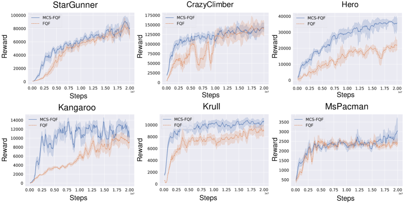
Figure 4: The performance curve on Atari games of MCS-FQF and baseline FQF models.

To illustrate the superiority of our proposed model, we conduct the experiments on Atari games and compare with vanilla FQF Yang et al. [2019]. Different from the FQF model implemented by DNN, the MCS-FQF model integrates more biologically plasubile mechaism such as multi-compartment neuron and population encoding, and is directly trained with surrogate gradient method. Thus, the comparative experiments could sufficiently demonstrate the advantages of brain-inspired model in enhancing information representation and integration.

The MCS-FQF model uses 512 multi-compartment neurons to integrates the states and quantile fractions. The final fully connected network consists of 512 neurons as a hidden layer and outputs the $N=32$ corresponding quantile values for each state-action pair. The MCS-FQF model is simulated with $T=8$ time steps and directly trained by the STBP algorithm with gradient surrogate function.

All models are learned with the same experimental settings, which can be found in Table S1, for 20 million frame steps. We use Adam optimizer to minimize the Huber quantile regression loss and RMSprop optimizer to minimize Wasserstein loss. We run ten rounds of the models’ tests, and the averaged reward and variance curve for our model and baseline are plotted in Figure 4. Experimental results show a consist performance boost of our MCF-FQF model on diverse games. Especially for the Hero, Kangroo and Krull games, our MCS-FQF model remarkably outperforms the baseline FQF model.

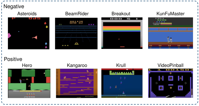
Figure S4: Game examples used in experiment. The top row shows the game in which the MCS-FQF model scores less than the FQF model. The bottom row shows the games in which the MCS-FQF model has achieved significant performance advantages.

The possible reason is that these three task scenarios are much complex, the enemies having elaborate shapes and behavior modes, the agent needing choose to attack or escape and also the game’s scenarios changing quickly over time as shown in Figure S4. This requires a stronger ability to integrate information, while the proposed MCS-FQF model with MCN exhibits better information integration capabilities, hence achieving significant superiority over FQF model. On the other three relatively simple tasks, which are designed with fixed scenes, enemies with the same form and a single behavior choice for the agent, our model achieves slight improvement on performance and accelerates learning. Overall, compared to the baseline FQF model, our MCS-FQF model learns faster and more stable, and achieves better performance on multiple games.

Comparing with ANN-SNN conversion based Spiking-FQF

Because there is no work applying the spiking neural network or multi-compartment neuron model to the DRL task, we choose to use the ANN-SNN conversion method convert the ANN in the FQF model to SNN and implement the Spiking-FQF model, which is one of the most stable and generalized methods that realize the application of deep spiking neural network on new tasks. We convert the trained FQF model to Spiking-FQF model by using the state-of-the-art ANN-SNN conversion method proposed by Li and Zeng [2022] with simulation time $T_{c}=256$ which guarantee the high performance of the Spiking-FQF model.

	FQF			ANN-SNN Conversion			MCS-FQF
Game	Score	$\pm$STD	(Score$\%$)	Score	$\pm$STD	(Score$\%$)	Score	$\pm$STD	(Score$\%$)
Asteroids	2292.0	812.9	(35.47$\%$)	1244.9	396.4	(31.84$\%$)	1666.0	718.4	(43.12$\%$)
Atlantis	2854490.0	40015.4	(1.40$\%$)	1571086.9	29768.5	(1.89$\%$)	3267690.0	120276.6	(3.68$\%$)
BeamRider	18192.0	9300.4	(51.12$\%$)	8227.6	3147.5	(38.25$\%$)	15302.2	6990.5	(45.68$\%$)
Bowling	59.7	0.9	(1.50$\%$)	37.7	3.1	(8.29$\%$)	63.5	8.5	(13.46$\%$)
Breakout	592.0	203.5	(34.38$\%$)	295.4	90.1	(30.51$\%$)	501.5	170.3	(33.96$\%$)
Centipede	7106.7	3617.9	(50.91$\%$)	5015.8	2199.2	(43.84$\%$)	7375.9	2929.6	(39.72$\%$)
CrazyClimber	157910.0	43971.0	(27.84$\%$)	2440.0	874.3	(35.83$\%$)	163010.0	21402.8	(13.13$\%$)
Enduro	3421.2	1274.0	(37.24$\%$)	2019.0	591.3	(29.29$\%$)	4156.4	874.7	(21.04$\%$)
Frostbite	7594.0	825.3	(10.87$\%$)	5269.9	797.9	(15.14$\%$)	8733.0	933.6	(10.69$\%$)
Hero	25709.5	16881.6	(65.66$\%$)	16851.7	1389.7	(8.25$\%$)	36912.5	1091.4	(2.96$\%$)
Kangaroo	11520.0	1647.3	(14.30$\%$)	7488.6	1248.4	(16.67$\%$)	15080.0	325.0	(2.15$\%$)
Krull	10207.0	773.0	(7.57$\%$)	6490.2	820.2	(12.64$\%$)	11276.0	599.5	(5.32$\%$)
KungFuMaster	44460.0	11357.1	(25.54$\%$)	18725.8	3506.5	(18.73$\%$)	34820.0	9692.9	(27.84$\%$)
MsPacman	3398.0	416.5	(12.26$\%$)	1761.9	650.2	(36.90$\%$)	3841.0	1269.7	(33.06$\%$)
Qbert	16515.0	621.5	(3.76$\%$)	8783.0	422.9	(4.82$\%$)	18042.5	1577.46	(8.74$\%$)
RoadRunner	53730.0	7760.4	(14.44$\%$)	26593.7	2458.9	(9.25$\%$)	52790.0	13469.5	(25.52$\%$)
StarGunner	97180.0	14331.4	(14.75$\%$)	56529.9	15062.0	(26.64$\%$)	103100.0	17266.19	(16.75$\%$)
Tutankham	267.9	10.5	(3.93$\%$)	157.9	15.9	(10.04$\%$)	298.5	37.0	(12.41$\%$)
VideoPinball	357333.9	282594.5	(79.08$\%$)	244185.7	203054.5	(83.16$\%$)	606765.7	250377.9	(41.26$\%$)

Table 1: Scores for Atari game experiments. The highest score for each game is bolded.

For the MCS-FQF model, the baseline FQF model, and the ANN-SNN conversion-based Spiking-FQF model, we conduct comparative experiments on 19 Atari games and record the mean scores, standard deviations (STD), and percentages of STD to Score (Score%) for ten trials, as shown in Table 1. The ANN-SNN conversion-based Spiking-FQF model is inferior to FQF model on all games, while our model achieves higher scores than FQF on most games. This illustrates the effectiveness of our SNN-based deep distributional RL model. In addition, the proposed MCS-FQF model shows a significant superiority over the conversion-based SNN model, indicating the effectiveness and robustness of our proposed direct training MCN model and population encoding method.

From Table 1, we find that the scores of our model are only slightly lower than the FQF model on 5 tasks and still significantly higher than the ANN-SNN conversion model. We analyzed why our MSF-FQF model does not perform as well as FQF in these games. Take the Asteroids, BeamRider and KungMaster as example, in which scores differ significantly between MCS-FQF model and vanilla FQF model, the game environment is relatively simple and the agent has few action choices, like ”left” or ”right” in Breakout. Comparing with this, the other 14 tasks is more complex as shown in Figure S4, and our model achieves best performance, especially on VideoPinball game, where our scores are about 1.7 $\times$ and 2.5 $\times$ higher than those of FQF and ANN-SNN conversion-based Spiking-FQF model, respectively. To sum up, our MCS-FQF model achieves comparable or even better performance compared to DNN-based FQF, and significantly outperforms the converted-based Spiking-FQF model on 19 Atari games.

The Effects of MCN and Population Encoding

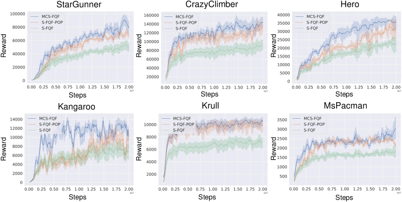
Figure 5: The effects of MCN and population encoding on models’ performance.

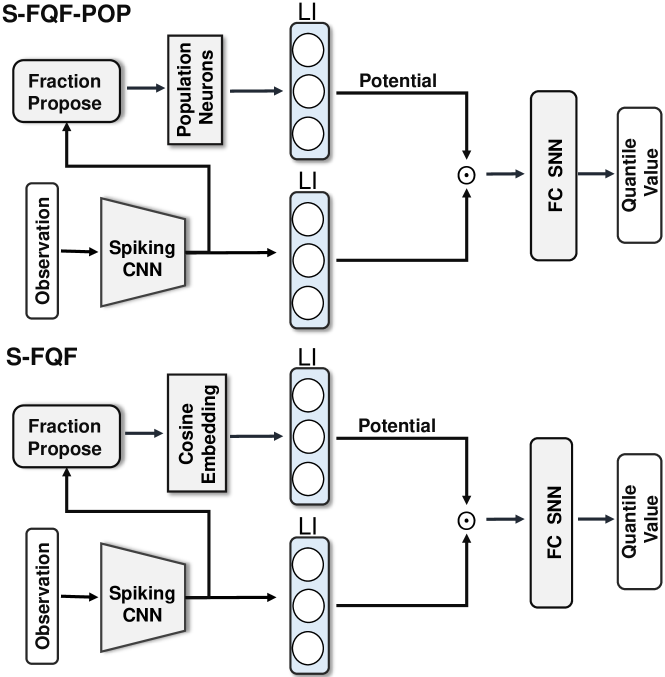
Figure S5: S-FQF-POP and S-FQF models in ablation study.

To further analyze the respective contributions of MCN and population encoding in the proposed model, we perform the model ablation studie on the Atari environment. We first replace the multi-compartment neuron module of MCS-FQF with Leaky-Integrate (LI) neuron and get the S-FQF-POP model, which can be seen as a directly training format of Spiking-FQF without MCN models. The LI neuron model is the LIF model without the spiking process, which uses the accumulated membrane potential $u(t)$ to transmit information. The SDQN model  Chen et al. [2022], which is trained directly by backpropagation, uses the membrane potential of LI neurons as the network output to represent state-action values. In the S-FQF-POP model, we use two groups of LI neuron models, each consisting of 512 LI neurons, to process state embedding spikes and quantile fraction embedding spikes respectively. Each step’s output membrane potentials $u(t)$ of these two groups of neurons are multiplied as the integration of state and fraction embedding. Then the fused information is input to the final fully connected SNN to generate quantile values. Except for replacing MCN with LI neuron, the rest of the S-FQF-POP is the same as the MCS-FQF model. Besides, we compare with the S-FQF model, which replaces the population encoding in the S-FQF-POP model with the cosine embedding as in FQF, to show the effect of population encoing method. The quantile fraction $\tau$ generated from state embedding spikes are represented by $cos(i\pi\tau)$ with $i\in\{0,1,...,M-1\}$. Figure S5 shows the structure of S-FQF-POP and S-FQF models.

	S-FQF			S-FQF-POP			MCS-FQF
Game	Score	$\pm$STD	(Score$\%$)	Score	$\pm$STD	(Score$\%$)	Score	$\pm$STD	(Score$\%$)
Asteroids	967.0	153.1	(15.83$\%$)	1517.0	406.5	(26.80$\%$)	1666.0	718.4	(43.12$\%$)
Atlantis	1545819.1	232356.4	(15.03$\%$)	2847970.0	42491.8	(1.49$\%$)	3267690.0	120276.6	(3.68$\%$)
BeamRider	8291.4	3400.6	(41.01$\%$)	12800.8	3922.3	(30.64$\%$)	15302.2	6990.5	(45.68$\%$)
Bowling	41.9	2.8	(6.67$\%$)	69.6	4.7	(6.75$\%$)	63.5	8.5	(13.46$\%$)
Breakout	280.9	123.9	(44.11$\%$)	419.8	119.3	(28.41$\%$)	501.5	170.3	(33.96$\%$)
Centipede	6619.1	2494.1	(37.68$\%$)	7979.1	2932.0	(36.75$\%$)	7375.9	2929.6	(39.72$\%$)
CrazyClimber	91873.3	23451.3	(25.53$\%$)	143020.0	19430.7	(13.59$\%$)	163010.0	21402.8	(13.13$\%$)
Enduro	1574.7	328.0	(20.83$\%$)	2965.4	1174.7	(39.61$\%$)	4156.4	874.7	(21.04$\%$)
Frostbite	3452.5	646.7	(18.73$\%$)	4889.0	894.6	(18.30$\%$)	8733.0	933.6	(10.69$\%$)
Hero	23576.8	348.6	(1.48$\%$)	36071.0	1390.9	(3.86$\%$)	36912.5	1091.4	(2.96$\%$)
Kangaroo	7111.6	1439.8	(20.25$\%$)	13100.0	2218.1	(16.93$\%$)	15080.0	325.0	(2.15$\%$)
Krull	9072.9	3149.9	(34.72$\%$)	11114.0	309.8	(2.79$\%$)	11276.0	599.5	(5.32$\%$)
KungFuMaster	20466.7	4120.2	(20.13$\%$)	35770.0	10032.2	(28.05$\%$)	34820.0	9692.9	(27.84$\%$)
MsPacman	1650.5	534.7	(32.40$\%$)	3017.0	1055.8	(34.99$\%$)	3841.0	1269.7	(33.06$\%$)
Qbert	8818.2	725.6	(8.23$\%$)	16355.0	1811.6	(11.08$\%$)	18042.5	1577.5	(8.74$\%$)
RoadRunner	32518.2	3813.8	(11.73$\%$)	50670.0	11126.9	(21.96$\%$)	52790.0	13469.5	(25.52$\%$)
StarGunner	43440.7	9515.0	(21.90$\%$)	80350.0	10540.8	(13.12$\%$)	103100.0	17266.19	(16.75$\%$)
Tutankham	104.6	20.7	(19.75$\%$)	214.4	27.3	(12.71$\%$)	298.5	37.0	(12.41$\%$)
VideoPinball	173795.0	170014.4	(97.82$\%$)	506845.2	226578.6	(44.70$\%$)	606765.7	250377.9	(41.26$\%$)

Table 2: Scores for ablation study. All models are run ten times with the same experimental settings.

We train all three models with the same parameter settings and run ten rounds of testing experiments for each model. The results are shown in Figure 5 and Table 2. Without MCN for information integration, the S-FQF-POP model shows performance degradation compared with MCS-FQF. And the population encoding method also plays a critical part in the model. The S-FQF learns more slowly and gets much small average scores than S-FQF-POP and MCS-FQF models.

Discussion

Compared with the baseline FQF model and the Spiking-FQF model based on ANN-SNN conversion, our proposed MCS-FQF model has performance advantages, and the ablation experiment proves that the multi-compartment neuron model and the population encoding method used in the model have important effect on the model’s information processing. In this section, we analyze the spiking activity of MCN in the learning process of the MCS-FQF model, and discuss the details of the cooperation between basal and apical dendrites of MCN in integrating information. According to the experimental results, we summarize the reasons for the better performance of MCS-FQF, and point out the limitations of this current study as well as the prospect of future work.

Analysis about the spiking activity of MCN

We recorded the multi-compartment neuron spiking activities when the trained model was tested on the MsPacman game to show the effect of basal dendrite and apical dendrite on the process of neuron making decision. A total of 128 multi-compartmental neurons in the MCS-FQF model were randomly selected, and their spiking activity was recorded over the testing trajectory.

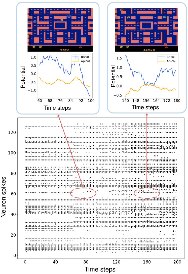
Figure 6: Records of multi-compartment neuron spikes and dendritic potential on experiments.

As shown in Figure 6, the multi-compartment neurons integrate state and quantile fraction information and have distinct spike sequences. The two block diagrams above of Figure 6 show the change in MCN basal and apical dendritic potentials. The block diagram on the left shows that the apical dendrites inhibit the effect of the basal dendrites on the somatic potential. When the potential of the basal dendrite is relatively high, due to the negative potential of the apical dendrite, there are not many neuronal spikes at this time.

In contrast, the block diagram on the right of Figure 6 shows that when the apical dendritic potential rises, even if the basal dendritic potential being small, the combined effects of the two compartments can increase the intensity of neuron spikes. We propose that this mechanisms of mutual inhibition and cooperation of neuron’s different parts promote the information computing power of a single neuron. SNNs with multi-compartment neurons can benefit from the more abundant and distinguishable neuronal spiking activities.

The ablation experiment shows that the neuron structure features play an important role in information integrating process, and the MCN model is better than the two group point neuron model combination as well as the pointwise value summation in FQF. We analyze the reason as the somatic potential of MCN integrates different source inputs from dendrites at the spatial-temporal level, as shown in Eq. (5). Its dynamic accumulation and decay mechanism are more powerful than point neuron models in processing the information represented by the spike sequences. Furthermore, compared with implicit cosine representations, encoding fractions with population spiking neurons can transform information into a high-dimensional space more suitable for spiking neural networks to distinguish.

We analyzed the factors affecting the performance of the proposed MCS-FQF model:

• Compared with the ReLU neurons in FQF, the spiking neuron model in MCS-FQF has more complex dynamic characteristics, which makes the model learn more information in the RL environment.

• Unlike pointwisely multiplying state embedding and fraction embedding in FQF and ANN-SNN conversion-based Spiking-FQF, MCS-FQF uses the multi-compartment neuron model to process them and has better information integrating capabilities.

• The directly trained MCS-FQF can learn better network weights than the Spiking-FQF model based on the ANN-SNN conversion.

• The population encoding method lets the quantile fraction information be more effectively represented in the spiking neural network.

Limitations of the study

When modeling the neuron structure, we only used the effect of dendritic potential on somatic potential, and does not include the characteristic of mutual interaction in dendrite and soma in biological neuron. Because, if containing mutual interaction of dendrite and soma in multi-compartment model, it introduces circle in computing graph, the MC neuron’s potential easily generate oscillation and exploding. Moreover, the backpropagation training method is not work for the computing circles. In future work, we will construct the MC neuron model including the somatic influence in dendrites and propose an efficient training method suiting to train SNNs with circle computing in more complex tasks. Besides, the proposed population neurons in this work has the same receptive field. How to use population neurons with different receptive fields and optimal activity to better represent spiking information is another problem that needs to be solved.

Conclusion

In this work, we propose a multi-compartment neuron model inspired from biological neuron structures, which uses dendrites to receive inputs from different sources and conduct the dendritic potential to the soma for information integration. And we apply multi-compartment spiking neural networks to deep distributional reinforcement learning and implement an SNN-based FQF model. The proposed MCS-FQF model implicitly represents quantile fractions into the spiking information space by using a Gaussian neuron population encoding method. The experiment results show that our model performs better than the vanilla FQF and the ANN-SNN conversion-based Spiking-FQF on 19 Atari game tests. In addition, we analyze the role of the proposed multi-compartment neuron and population encoding methods in the model. The ablation study shows that both of them improve the performance of spiking neural networks in distributional reinforcement learning. Compared with ANNs, brain-inspired spiking neural networks are more functional in information processing with better biological plausibility. In this paper, we introduce the structural details and information encoding characteristics of biological neurons to SNN-based reinforcement learning models, and improve the spiking neural network’s capability to handle complex learning tasks. Moreover, we hope our works will also contribute to the better neuromorphic computing model explorations.

Resource availability

Lead contact

Further information and requests for resources and reagents should be directed to and will be fulfilled by the lead contact, Yi Zeng (yi.zeng@ia.ac.cn).

Materials availability

This study did not generate new unique reagents.

Data and code availability

The Python scripts can be downloaded from the GitHub repository: https://github.com/BrainCog-X/Brain-Cog/tree/dev/examples/decision_making/RL/mcs-fqf

Supplementary Material

Proof 1

This is proof of Theory 1.

The MCN membrane potential equation

$$\tau_{L}\frac{du}{dt}=-u(t)+\frac{g_{B}}{g_{L}}(V^{b}(t)-u(t))+\frac{g_{A}}{g_{L}}(V^{a}(t)-u(t))$$ (32)

can be rewritten as

$$\frac{du}{dt}+Zu(t)+C(t)=0$$ (33)

$$Z=\frac{g_{B}+g_{A}+g_{L}}{\tau_{L}g_{L}}$$ (34)

$$C(t)=-\frac{1}{\tau_{L}}[\frac{g_{B}}{g_{L}}V^{b}(t)+\frac{g_{A}}{g_{L}}V^{a}(t)]$$ (35)

This is a first-order linear differential equation, and its general solution is

$$u(t)=A(t)e^{-\int Zdt}=A(t)e^{-Zt}$$ (36)

Substituting the solution for $u(t)$ of Eq. (36) into Eq. (33), we get

$$A(t)=\int-e^{Zt}C(t)dt$$ (37)

Thus, $u(t)$ is solved as

$$u(t)=\int^{t}_{-\infty}\frac{e^{Zt}}{\tau_{L}}[\frac{g_{B}}{g_{L}}V^{b}(t)+\frac{g_{A}}{g_{L}}V^{a}(t)]dte^{-Zt}.$$ (38)

Parameter	Value	Description	Parameter	Value	Description
$\tau_{L}$	2.0	Decay constant	$N$	32	Fraction number
$V_{th}$	1.0	Threshold potential	$M$	64	Population number
$V_{reset}$	0.0	Reset potential	$C$	0.05	receptive constant
$T$	8	Simulation Times	$lr_{a}$	$1.0e^{-4}$	Adam learning rate
$\tau_{A}$	2.0	Apical constant	$lr_{f}$	$2.5e^{-9}$	RMSprop learning rate
$\tau_{B}$	2.0	Basal constant
$g_{A}$	1.0	Apical conductance
$g_{B}$	1.0	Basal conductance
$g_{L}$	1.0	Leaky conductance

Table T1: Parameter settings for experiments.

References

- Balachandar and Michmizos [2020] Balachandar, P., Michmizos, K.P., 2020. A spiking neural network emulating the structure of the oculomotor system requires no learning to control a biomimetic robotic head, in: 2020 8th IEEE RAS/EMBS International Conference for Biomedical Robotics and Biomechatronics (BioRob), IEEE. pp. 1128–1133.
- Capone et al. [2022] Capone, C., Lupo, C., Muratore, P., Paolucci, P.S., 2022. Burst-dependent plasticity and dendritic amplification support target-based learning and hierarchical imitation learning. arXiv preprint arXiv:2201.11717 .
- Chen et al. [2022] Chen, D., Peng, P., Huang, T., Tian, Y., 2022. Deep reinforcement learning with spiking q-learning. arXiv preprint arXiv:2201.09754 .
- Davies et al. [2018] Davies, M., Srinivasa, N., Lin, T.H., Chinya, G., Cao, Y., Choday, S.H., Dimou, G., Joshi, P., Imam, N., Jain, S., et al., 2018. Loihi: A neuromorphic manycore processor with on-chip learning. Ieee Micro 38, 82–99.
- Dominguez-Morales et al. [2018] Dominguez-Morales, J.P., Liu, Q., James, R., Gutierrez-Galan, D., Jimenez-Fernandez, A., Davidson, S., Furber, S., 2018. Deep spiking neural network model for time-variant signals classification: a real-time speech recognition approach, in: 2018 International Joint Conference on Neural Networks (IJCNN), IEEE. pp. 1–8.
- Furber et al. [2014] Furber, S.B., Galluppi, F., Temple, S., Plana, L.A., 2014. The spinnaker project. Proceedings of the IEEE 102, 652–665.
- Gerstner and Kistler [2002] Gerstner, W., Kistler, W.M., 2002. Spiking neuron models: Single neurons, populations, plasticity. Cambridge university press.
- Gidon et al. [2020] Gidon, A., Zolnik, T.A., Fidzinski, P., Bolduan, F., Papoutsi, A., Poirazi, P., Holtkamp, M., Vida, I., Larkum, M.E., 2020. Dendritic action potentials and computation in human layer 2/3 cortical neurons. Science 367, 83–87.
- Hodgkin et al. [1952] Hodgkin, A.L., Huxley, A.F., Katz, B., 1952. Measurement of current-voltage relations in the membrane of the giant axon of loligo. The Journal of physiology 116, 424.
- Huber [1992] Huber, P.J., 1992. Robust estimation of a location parameter, in: Breakthroughs in statistics. Springer, pp. 492–518.
- Izhikevich [2004] Izhikevich, E.M., 2004. Which model to use for cortical spiking neurons? IEEE transactions on neural networks 15, 1063–1070.
- Kakei et al. [1999] Kakei, S., Hoffman, D.S., Strick, P.L., 1999. Muscle and movement representations in the primary motor cortex. Science 285, 2136–2139.
- Kampa and Stuart [2006] Kampa, B.M., Stuart, G.J., 2006. Calcium spikes in basal dendrites of layer 5 pyramidal neurons during action potential bursts. Journal of Neuroscience 26, 7424–7432.
- Kim et al. [2020] Kim, S., Park, S., Na, B., Yoon, S., 2020. Spiking-yolo: spiking neural network for energy-efficient object detection, in: Proceedings of the AAAI conference on artificial intelligence, pp. 11270–11277.
- Kopsick et al. [2022] Kopsick, J.D., Tecuatl, C., Moradi, K., Attili, S.M., Kashyap, H.J., Xing, J., Chen, K., Krichmar, J.L., Ascoli, G.A., 2022. Robust resting-state dynamics in a large-scale spiking neural network model of area ca3 in the mouse hippocampus. Cognitive Computation , 1–21.
- Lansdell et al. [2019] Lansdell, B.J., Prakash, P.R., Kording, K.P., 2019. Learning to solve the credit assignment problem. arXiv preprint arXiv:1906.00889 .
- Lee et al. [2020] Lee, C., Sarwar, S.S., Panda, P., Srinivasan, G., Roy, K., 2020. Enabling spike-based backpropagation for training deep neural network architectures. Frontiers in neuroscience , 119.
- Li and Zeng [2022] Li, Y., Zeng, Y., 2022. Efficient and accurate conversion of spiking neural network with burst spikes. arXiv preprint arXiv:2204.13271 .
- Liu et al. [2021] Liu, G., Deng, W., Xie, X., Huang, L., Tang, H., 2021. Human-level control through directly-trained deep spiking q-networks. arXiv preprint arXiv:2201.07211 .
- Lowet et al. [2020] Lowet, A.S., Zheng, Q., Matias, S., Drugowitsch, J., Uchida, N., 2020. Distributional reinforcement learning in the brain. Trends in Neurosciences 43, 980–997.
- Luo et al. [2021] Luo, Y., Xu, M., Yuan, C., Cao, X., Zhang, L., Xu, Y., Wang, T., Feng, Q., 2021. Siamsnn: siamese spiking neural networks for energy-efficient object tracking, in: International Conference on Artificial Neural Networks, Springer. pp. 182–194.
- Makara and Magee [2013] Makara, J.K., Magee, J.C., 2013. Variable dendritic integration in hippocampal ca3 pyramidal neurons. Neuron 80, 1438–1450.
- Merolla et al. [2014] Merolla, P.A., Arthur, J.V., Alvarez-Icaza, R., Cassidy, A.S., Sawada, J., Akopyan, F., Jackson, B.L., Imam, N., Guo, C., Nakamura, Y., et al., 2014. A million spiking-neuron integrated circuit with a scalable communication network and interface. Science 345, 668–673.
- Meyers [2018] Meyers, E.M., 2018. Dynamic population coding and its relationship to working memory. Journal of neurophysiology 120, 2260–2268.
- Panzeri et al. [2015] Panzeri, S., Macke, J.H., Gross, J., Kayser, C., 2015. Neural population coding: combining insights from microscopic and mass signals. Trends in Cognitive Sciences 19, 162–172. URL: https://www.sciencedirect.com/science/article/pii/S1364661315000030, doi:https://doi.org/10.1016/j.tics.2015.01.002.
- Poirazi et al. [2003] Poirazi, P., Brannon, T., Mel, B.W., 2003. Pyramidal neuron as two-layer neural network. Neuron 37, 989–999.
- Polsky et al. [2004] Polsky, A., Mel, B.W., Schiller, J., 2004. Computational subunits in thin dendrites of pyramidal cells. Nature neuroscience 7, 621–627.
- Ponghiran and Roy [2022] Ponghiran, W., Roy, K., 2022. Spiking neural networks with improved inherent recurrence dynamics for sequential learning, in: Proceedings of the AAAI Conference on Artificial Intelligence, pp. 8001–8008.
- Richards et al. [2019] Richards, B.A., Lillicrap, T.P., Beaudoin, P., Bengio, Y., Bogacz, R., Christensen, A., Clopath, C., Costa, R.P., de Berker, A., Ganguli, S., et al., 2019. A deep learning framework for neuroscience. Nature neuroscience 22, 1761–1770.
- Sacramento et al. [2018] Sacramento, J., Ponte Costa, R., Bengio, Y., Senn, W., 2018. Dendritic cortical microcircuits approximate the backpropagation algorithm. Advances in neural information processing systems 31.
- Sanger [2003] Sanger, T.D., 2003. Neural population codes. Current Opinion in Neurobiology 13, 238–249. URL: https://www.sciencedirect.com/science/article/pii/S0959438803000345, doi:https://doi.org/10.1016/S0959-4388(03)00034-5.
- Shivkumar et al. [2018] Shivkumar, S., Lange, R., Chattoraj, A., Haefner, R., 2018. A probabilistic population code based on neural samples, in: Bengio, S., Wallach, H., Larochelle, H., Grauman, K., Cesa-Bianchi, N., Garnett, R. (Eds.), Advances in Neural Information Processing Systems, Curran Associates, Inc. URL: https://proceedings.neurips.cc/paper/2018/file/5401acfe633e6817b508b84d23686743-Paper.pdf.
- Shrestha et al. [2021] Shrestha, A., Fang, H., Rider, D.P., Mei, Z., Qiu, Q., 2021. In-hardware learning of multilayer spiking neural networks on a neuromorphic processor, in: 2021 58th ACM/IEEE Design Automation Conference (DAC), pp. 367–372. doi:10.1109/DAC18074.2021.9586323.
- Smith et al. [2013] Smith, S.L., Smith, I.T., Branco, T., Häusser, M., 2013. Dendritic spikes enhance stimulus selectivity in cortical neurons in vivo. Nature 503, 115–120.
- Sun et al. [2022] Sun, Y., Zeng, Y., Li, Y., 2022. Solving the spike feature information vanishing problem in spiking deep q network with potential based normalization. Frontiers in Neuroscience 16. URL: https://www.frontiersin.org/articles/10.3389/fnins.2022.953368, doi:10.3389/fnins.2022.953368.
- Tan et al. [2021] Tan, W., Patel, D., Kozma, R., 2021. Strategy and benchmark for converting deep q-networks to event-driven spiking neural networks, in: Proceedings of the AAAI conference on artificial intelligence, pp. 9816–9824.
- Tang et al. [2020a] Tang, G., Kumar, N., Michmizos, K.P., 2020a. Reinforcement co-learning of deep and spiking neural networks for energy-efficient mapless navigation with neuromorphic hardware, in: 2020 IEEE/RSJ International Conference on Intelligent Robots and Systems (IROS), IEEE. pp. 6090–6097.
- Tang et al. [2020b] Tang, G., Kumar, N., Yoo, R., Michmizos, K.P., 2020b. Deep reinforcement learning with population-coded spiking neural network for continuous control. arXiv preprint arXiv:2010.09635 .
- Urbanczik and Senn [2014] Urbanczik, R., Senn, W., 2014. Learning by the dendritic prediction of somatic spiking. Neuron 81, 521–528.
- Vaila [2021] Vaila, R., 2021. Deep convolutional spiking neural networks for image classification. Boise State University.
- Wu et al. [2018] Wu, Y., Deng, L., Li, G., Zhu, J., Shi, L., 2018. Spatio-temporal backpropagation for training high-performance spiking neural networks. Frontiers in Neuroscience 12. URL: https://www.frontiersin.org/article/10.3389/fnins.2018.00331, doi:10.3389/fnins.2018.00331.
- Yang et al. [2019] Yang, D., Zhao, L., Lin, Z., Qin, T., Bian, J., Liu, T.Y., 2019. Fully parameterized quantile function for distributional reinforcement learning. Advances in neural information processing systems 32.
- Zhang et al. [2021] Zhang, L., Cao, J., Zhang, Y., Zhou, B., Feng, S., 2021. Distilling neuron spike with high temperature in reinforcement learning agents. arXiv preprint arXiv:2108.10078 .
- Zhao et al. [2018] Zhao, F., Zeng, Y., Xu, B., 2018. A brain-inspired decision-making spiking neural network and its application in unmanned aerial vehicle. Frontiers in neurorobotics 12, 56.