Additive Schwarz methods for fourth-order variational inequalities

Abstract

We consider additive Schwarz methods for fourth-order variational inequalities. While most existing works on Schwarz methods for fourth-order variational inequalities deal with auxiliary linear problems instead of the original ones, we deal with the original ones directly by using a nonlinear subspace correction framework for convex optimization. Based on a unified framework of various finite element methods for fourth-order variational inequalities, we develop one- and two-level additive Schwarz methods. We prove that the two-level method is scalable in the sense that the convergence rate of the method depends on $H/h$ and $H/\delta$ only, where $h$ and $H$ are the typical diameters of an element and a subdomain, respectively, and $\delta$ measures the overlap among the subdomains. To the best of our knowledge, the proposed two-level method is the first scalable Schwarz method for fourth-order variational inequalities. An efficient numerical method to solve coarse problems in the two-level method is also presented. Our theoretical results are verified by numerical experiments.

65N55, 65K15, 65N30, 49M27

1 Introduction

This paper is concerned with scalable parallel algorithms to solve fourth-order variational problems. Let $\Omega\subset\mathbb{R}^{2}$ be a convex polygonal domain and $S$ be a subspace of $H^{2}(\Omega)$ with a boundary condition that makes the Poincaré–Friedrichs inequality hold [31]. As a model problem, we consider the constrained optimization problem:

(1) $$\min_{u\in K}\left\{\frac{1}{2}a(u,u)-(f,u)\right\},$$

where $a(\cdot,\cdot)$ is a continuous and coercive bilinear form on $S$ derived from a fourth-order elliptic problem, $(\cdot,\cdot)$ is the standard $L^{2}(\Omega)$-inner product, and the constraint set $K$ is given by

$$K=\left\{u\in S:u\leq\psi\textrm{ in }\Omega\right\}$$

for some $\psi\in C(\overline{\Omega})\cap C^{2}(\Omega)$. It is well-known that Eq. 1 admits an equivalent fourth-order variational inequality formulation [14, 17]: find $u^{*}\in K$ such that

(2) $$a(u^{*},u-u^{*})\geq(f,u-u^{*})\quad\forall u\in K.$$

Since Eq. 1 and Eq. 2 are equivalent, we refer to the optimization problem Eq. 1 as a fourth-order variational inequality as well throughout this paper.

Problems of the form either Eq. 1 or Eq. 2 appear in diverse fields of science and engineering. For example, if we set

(3) $$S=H_{0}^{2}(\Omega),\quad a(u,v)=\int_{\Omega}\nabla^{2}u:\nabla^{2}v\,dx,$$

where $\nabla^{2}$ and $:$ denote the Hessian and the Frobenius inner product, respectively, then we obtain the displacement obstacle problem of clamped plates [12, 16, 17]. On the other hand, if we set

(4) $$S=H^{2}(\Omega)\cap H_{0}^{1}(\Omega),\quad a(u,v)=\int_{\Omega}(\beta\nabla^{2}u:\nabla^{2}v+uv)\,dx$$

for some $\beta>0$, then we get the elliptic distributed optimal control problem with pointwise constraints introduced in [14, 20, 30]. Various finite element discretizations for either Eq. 1 or Eq. 2 have been considered in a number of existing works: nonconforming methods [30], mixed methods [23], partition of unity methods [11], discontinuous Galerkin methods [13, 21], and virtual element methods [15]. In particular, unified frameworks for finite element methods including $C^{1}$ conforming methods, nonconforming methods, and discontinuous Galerkin methods were proposed in [14, 17].

We consider domain decomposition methods [41] as parallel numerical solvers for the fourth-order variational inequality Eq. 1. We were motivated by some interesting literature on domain decomposition methods for optimization problems of the form Eq. 1 and variational inequalities of the form Eq. 2. Schwarz methods for second-order variational inequalities of the form Eq. 2 were considered in [3, 4, 37], and then generalized to variational inequalities of the second kind and quasi-variational inequalities in [2]. A dual-primal nonoverlapping domain decomposition method for variational inequalities appearing in structural mechanics was proposed in [27]. Recently, the linear convergence of Schwarz methods for variational inequalities involving the $p$-Laplacian was analyzed in [29]. Meanwhile, the convergence theory of Schwarz methods for smooth convex optimization problems was developed in [40], and then extended to constrained and nonsmooth problems in [1] and [34], respectively.

In this paper, we present and analyze additive Schwarz methods for the fourth-order variational inequality Eq. 1. On the contrary that several existing works [12, 16] on additive Schwarz methods for Eq. 1 and Eq. 2 deal with auxiliary linear problems appearing in a primal-dual active set method [6, 24], our proposed methods are based on the nonlinear subspace correction framework for convex optimization problems presented in [1, 34, 40]. That is, each subdomain problem in the proposed methods is nonlinear and has the same form as the full-dimensional problem Eq. 1.

Based on a unified framework [14] of various finite element methods for Eq. 1 including $C^{1}$ finite element methods [43], nonconforming finite element methods [10], and discontinuous Galerkin methods [18], we develop a one-level additive Schwarz method and prove that its additive Schwarz condition number [34] is $O(1/H\delta^{3})$, where $H$ denotes the subdomain diameter and $\delta$ measures the overlap among the subdomains. This estimate is the same as those of one-level additive Schwarz methods for the auxiliary linear problems considered in [12, 16]. In addition, inspired by the partition of unity method for fourth-order elliptic problems [11, 12], we propose a novel coarse space suitable for the constrained problem Eq. 1. We show that the additive Schwarz condition number of a two-level additive Schwarz method equipped with the proposed coarse space is bounded by $O(C(H,h)(H/\delta)^{3})$, where $h$ is the diameter of fine elements and $C(H,h)$ a positive constant depending on $H/h$ only. We remark that, while designing appropriate coarse spaces for second-order variational inequalities was successfully done in several existing works [1, 3, 37], the case of higher-order problems such as Eq. 1 has been regarded as a rather challenging task (see, e.g., [32, 38]). To the best of our knowledge, the proposed coarse space is the first one that yields a scalable domain decomposition method for fourth-order variational inequalities.

This paper is organized as follows. In Section 2, we introduce finite element discretizations and additive Schwarz methods for the fourth-order variational inequality Eq. 1. In Section 3, we present a one-level additive Schwarz method for Eq. 1. In Section 4, we propose a novel partition of unity coarse space for Eq. 1 and analyze a two-level additive Schwarz method equipped with the proposed coarse space. In Section 5, we discuss about efficient numerical methods for local and coarse problems in the proposed additive Schwarz methods. In Section 6. we present numerical results that support our theoretical results. We conclude this paper with remarks in Section 7.

2 Preliminaries

In this section, we provide preliminaries for this paper, which are mainly borrowed from [14, 34]. We introduce finite element discretizations of the fourth-order variational inequality Eq. 1. Then, we present a general additive Schwarz method for the fourth-order variational inequality based on an abstract space decomposition.

In what follows, we use the notation $A\lesssim B$ and $B\gtrsim A$ to represent that there exists a constant $c>0$ such that $A\leq cB$, where $c$ is independent of the parameters $h$, $H$, and $\delta$ relying on discretization and domain decomposition. The notation $A\approx B$ means that $A\lesssim B$ and $A\gtrsim B$.

2.1 Finite element discretizations

We present a unified framework of finite element methods for the fourth-order variational inequality Eq. 1, where similar frameworks were introduced in [14, 17]. This framework can deal with various finite element methods for fourth-order problems such as $C^{1}$ finite element methods, nonconforming finite element methods, and discontinuous Galerkin methods. One may refer to [43] and [10] for various examples of $C^{1}$ conforming and nonconforming finite elements, respectively.

Let $\mathcal{T}_{h}$ be a quasi-uniform triangulation of $\Omega$ with $h$ the characteristic element diameter. Assume that we have the followings:

• a finite element space $S_{h}\subset L^{2}(\Omega)$ defined on $\mathcal{T}_{h}$,

• a norm $\|\cdot\|_{h}$ defined on $S_{h}+S$,

• a symmetric bilinear form $a_{h}(\cdot,\cdot)$ on $S_{h}$,

• an interpolation operator $\Pi_{h}$ onto $S_{h}$,

• an enriching operator $E_{h}$ that maps $S_{h}$ to a conforming finite element space $\widetilde{S}_{h}\subset S$.

We also assume that every function in $S_{h}$ is continuous at the vertices of $\mathcal{T}_{h}$ so that the following constraint set $K_{h}\subset S_{h}$ is well-defined:

$$K_{h}=\left\{u\in S_{h}:u\leq\psi\textrm{ at the vertices of }\mathcal{T}_{h}\right\}.$$

Under the above assumptions, the following finite element approximation of Eq. 1 defined on $S_{h}$ can be considered:

(5) $$\min_{u\in K_{h}}\left\{F_{h}(u):=\frac{1}{2}a_{h}(u,u)-(f,u)\right\}.$$

In the convergence analysis of additive Schwarz methods that will be introduced in this paper, we require several assumptions on $\|\cdot\|_{h}$, $a_{h}(\cdot,\cdot)$, $\Pi_{h}$, and $E_{h}$; these assumptions are valid for various finite element methods for Eq. 1 including all the ones covered in [14, 17]. First, we assume that the norm $\|\cdot\|_{h}$ and the bilinear form $a_{h}(\cdot,\cdot)$ are chosen such that

(6) $$a_{h}(u,u)\approx\|u\|_{h}^{2},\quad u\in S_{h},$$

i.e., $a_{h}(\cdot,\cdot)$ is equivalent to $\|\cdot\|_{h}^{2}$ in $S_{h}$ (cf. [14, equations (3.4) and (3.5)]). The interpolation operator $\Pi_{h}$ is a projection onto $S_{h}$, i.e.,

(7) $$\Pi_{h}u=u,\quad u\in S_{h},$$

and it is assumed to satisfy the following approximation and stability estimate:

(8) $$\|\zeta-\Pi_{h}\zeta\|_{L^{2}(\Omega)}+h\left(\sum_{T\in\mathcal{T}_{h}}|\zeta-\Pi_{h}\zeta|_{H^{1}(T)}^{2}\right)^{\frac{1}{2}}+h^{2}\|\Pi_{h}\zeta\|_{h}\lesssim h^{2}|\zeta|_{H^{2}(\Omega)},\hskip 2.84544pt\zeta\in S.$$

Moreover, it should preserve the function values at the vertices of $\mathcal{T}_{h}$, i.e.,

(9) $$\Pi_{h}\zeta=\zeta\text{ at the vertices of }\mathcal{T}_{h},\quad\zeta\in S.$$

Interpolation operators satisfying Eqs. 7, 8, and 9 for various finite element methods can be found in, e.g., [10, Lemma 3.1], [12, equation (2.3)], and [16, Lemma 4.1]. Finally, we assume that the enriching operator $E_{h}$ satisfies

(10) $$\|u-E_{h}u\|_{L^{2}(\Omega)}+h\left(\sum_{T\in\mathcal{T}_{h}}|u-E_{h}u|_{H^{1}(T)}^{2}\right)^{\frac{1}{2}}+h^{2}|E_{h}u|_{H^{2}(\Omega)}\lesssim h^{2}\|u\|_{h},\quad u\in S_{h},$$

and that it preserves the function values at the vertices of $\mathcal{T}_{h}$ (cf. [14, equations (3.10) and (3.11)]):

(11) $$E_{h}u=u\text{ at the vertices of }\mathcal{T}_{h},\quad u\in S_{h}.$$

Thanks to Eq. 6, the energy functional $F_{h}$ of Eq. 5 is strongly convex. Hence, Eq. 5 admits a unique solution $u_{h}\in K_{h}$. An error estimate between $u_{h}$ and the solution of the continuous problem Eq. 1 under some elliptic regularity condition can be found in [17, Theorem 4.2] and [14, Theorem 4.1].

2.2 Additive Schwarz method

We introduce a general additive Schwarz method for the discrete fourth-order variational inequality Eq. 5 based on an abstract space decomposition for the solution space $V=S_{h}$. We assume that there exist finite-dimensional spaces $V_{k}$, $1\leq k\leq N$, and bounded linear operators $R_{k}^{*}\colon V_{k}\rightarrow V$ such that

(12) $$V=\sum_{k=1}^{N}R_{k}^{*}V_{k}.$$

Note that $V_{k}$ need not be a subspace of $V$. A stable decomposition assumption [34, Assumption 4.1] associated with Eq. 12 for the problem Eq. 5 is stated below.

[stable decomposition] There exists a constant $C_{0}$ such that for any $u,v\in K_{h}$, $u-v$ admits a decomposition

$$u-v=\sum_{k=1}^{N}R_{k}^{*}w_{k},\quad w_{k}\in V_{k},\hskip 2.84544pt1\leq k\leq N,$$

that satisfies $v+R_{k}^{*}w_{k}\in K_{h}$ and

$$\sum_{k=1}^{N}a_{h}(R_{k}^{*}w_{k},R_{k}^{*}w_{k})\leq\frac{C_{0}^{2}}{2}\|u-v\|_{h}^{2}.$$

The abstract additive Schwarz method for Eq. 5 under the space decomposition Eq. 12 is presented in Algorithm 1. We note that the same algorithm appeared in several existing works [4, 34, 39]. The constant $\tau_{0}$ in Algorithm 1 is usually chosen as $\tau_{0}=1/N_{c}$, where $N_{c}$ is the minimum number of classes that is required to classify the spaces $\{V_{k}\}_{k=1}^{N}$ by the usual coloring technique [34, section 5.1].

Algorithm 1 Abstract additive Schwarz method for Eq. 5

  Choose $u^{(0)}\in K_{h}$ and $\tau\in(0,\tau_{0}]$.

  for $n=0,1,2,\dots$ do

     

$$\begin{split}w_{k}^{(n+1)}&\in\operatorname*{\arg\min}_{\begin{subarray}{c}w_{k}\in V_{k},\\ u^{(n)}+R_{k}^{*}w_{k}\in K_{h}\end{subarray}}F_{h}\left(u^{(n)}+R_{k}^{*}w_{k}\right),\quad 1\leq k\leq N,\\ u^{(n+1)}&=u^{(n)}+\tau\sum_{k=1}^{N}R_{k}^{*}w_{k}^{(n+1)}\end{split}$$

  end for

Invoking Eq. 6 and Section 2.2, one can prove the linear convergence of Algorithm 1; we state the convergence theorem by Park [34, Theorem 4.8] in a form suitable for our purposes.

Theorem 2.1.

Assume that Section 2.2 holds. In Algorithm 1, we have

$$\frac{F_{h}(u^{(n+1)})-F_{h}(u_{h})}{F_{h}(u^{(n)})-F_{h}(u_{h})}\\ \leq 1-\gamma^{-1},\quad n\geq 0,$$

where $\gamma>1$ is a constant that satisfies

$$\gamma\lesssim\frac{C_{0}^{2}}{\tau}.$$

Proof 2.2.

In [34], the following four conditions were considered to ensure the linear convergence of the general additive Schwarz method: stable decomposition, strengthened convexity, local stability, and sharpness [34, Assumptions 4.1–4.3 and 3.4]. Among them, strengthened convexity and local stability obviously hold. Sharpness of the energy functional $F$ follows from Eq. 6. Hence, verifying Section 2.2, the stable decomposition condition, is enough to obtain the desired result.

Thanks to Theorem 2.1, it suffices to prove Section 2.2 in order for the convergence analysis of Algorithm 1. In Sections 3 and 4, we will estimate the constant $C_{0}^{2}$ in Section 2.2 corresponding to one- and two-level domain decomposition settings in terms of the parameters $h$, $H$, and $\delta$, respectively.

Remark 2.3.

The practical performance of Algorithm 1 can be improved by adopting some acceleration schemes designed for first-order methods for convex optimization. If we combine Algorithm 1 with an acceleration scheme so called FISTA [5] with adaptive restart [33], then we obtain the accelerated additive Schwarz method proposed in [35]. The idea of full backtracking proposed in [19] can be incorporated with Algorithm 1 to improve the convergence rate [36]. However, we will not cover these accelerated variants since they are beyond the scope of this paper.

3 One-level method

In this section, we present a one-level additive Schwarz method for the discrete fourth-order variational inequality Eq. 5 based on an overlapping domain decomposition setting. Then we provide a convergence analysis of the one-level method. The convergence result given in this section is applicable to any finite element methods that can be interpreted in the unified framework introduced in Section 2.

3.1 Domain decomposition

Let $\mathcal{T}_{H}$ be a quasi-uniform triangulation of $\Omega$ such that $\mathcal{T}_{h}$ is a refinement of $\mathcal{T}_{H}$, where $H$ stands for the characteristic element diameter of $\mathcal{T}_{H}$. Two triangulations $\mathcal{T}_{h}$ and $\mathcal{T}_{H}$ will play roles of fine and coarse meshes, respectively. We assume that the domain $\Omega$ is decomposed into a collection of overlapping subdomains $\{\Omega_{k}\}_{k=1}^{N}$ such that each $\Omega_{k}$ is a union of elements in $\mathcal{T}_{h}$ and $\operatorname{diam}\Omega_{k}\approx H$. The overlap width among the subdomains is denoted by $\delta$.

As in [10, 18, 43], we assume that the overlapping domain decomposition $\{\Omega_{k}\}_{k=1}^{N}$ admits a $W^{2,\infty}$-partition of unity $\{\theta_{k}\}_{k=1}^{N}$ such that

(13a) $$\theta_{k}=0\quad\text{ on }\Omega\setminus\Omega_{k},$$

(13b) $$\sum_{k=1}^{N}\theta_{k}=1\quad\text{ on }\overline{\Omega},$$

(13c) $$\|\nabla\theta_{k}\|_{L^{\infty}(\Omega_{k})}\lesssim\frac{1}{\delta},\hskip 2.84544pt\|\nabla^{2}\theta_{k}\|_{L^{\infty}(\Omega_{k})}\lesssim\frac{1}{\delta^{2}}, \quad 1\leq k\leq N.$$

We assume that $\{\theta_{k}\}_{k=1}^{N}$ satisfies

(14) $$\sum_{k=1}^{N}\|\Pi_{h}(\theta_{k}u)\|_{h}^{2}\lesssim\|u\|_{h}^{2}+\frac{1}{\delta^{2}}\sum_{T\in\mathcal{T}_{h}}|u|_{H^{1}(T)}^{2}\\ +\frac{1}{H\delta^{3}}\|E_{h}u\|_{L^{2}(\Omega)}^{2}+\left(\frac{H}{\delta}\right)^{3}|E_{h}u|_{H^{2}(\Omega)}^{2},\hskip 2.84544ptu\in S_{h}.$$

The estimate Eq. 14 is usually derived using Eq. 8 and Eq. 13c. In particular, the last two terms in Eq. 14 can be obtained by a trace theorem-type argument introduced in [22]. One may refer to [10, section 8] and [18, section 5] for details for nonconforming finite element methods and discontinuous Galerkin methods, respectively; see also [12, Remark 5.3] and [16, Remark 4.2].

In Algorithm 1, we set $V=S_{h}$ and

$$V_{k}=S_{h}(\Omega_{k}),\quad 1\leq k\leq N,$$

where $S_{h}(\Omega_{k})$ is the finite element space of the same type as $S_{h}$ defined on $\Omega_{k}$. The operator $R_{k}^{*}\colon V_{k}\rightarrow V$, $1\leq k\leq N$, is given by the natural extension operator from $S_{h}(\Omega_{k})$ to $S_{h}$. Then we obtain the desired one-level additive Schwarz method for Eq. 5.

3.2 Convergence analysis

As we discussed in Section 2, it suffices to estimate the constant $C_{0}^{2}$ in Section 2.2 in order to analyze the convergence rate of the one-level additive Schwarz method. By a similar argument as [12, Theorem 5.1] and [16, Lemma 4.3], one can prove Theorem 3.1, which provides an estimate for $C_{0}^{2}$.

Theorem 3.1.

In the space decomposition Eq. 12, Section 2.2 holds with

$$C_{0}^{2}\approx\frac{1}{H\delta^{3}}.$$

Proof 3.2.

Take any $u,v\in K_{h}$ and let $w=u-v$. We define $w_{k}\in V_{k}$, $1\leq k\leq N$, as

$$w_{k}=\Pi_{h}(\theta_{k}w),$$

where $\{\theta_{k}\}_{k=1}^{N}$ is the partition of unity given in Eq. 13. Then, by Eq. 7, we readily have $w=\sum_{k=1}^{N}R_{k}^{*}w_{k}$. Moreover, Eq. 9 implies that $v+R_{k}^{*}w_{k}\in K_{h}$. By Eqs. 6 and 14, we get

(15) $$\sum_{k=1}^{N}a_{h}(R_{k}^{*}w_{k},R_{k}^{*}w_{k})\approx\sum_{k=1}^{N}\|R_{k}^{*}w_{k}\|_{h}^{2}\\ \lesssim\|w\|_{h}^{2}+\frac{1}{\delta^{2}}\sum_{T\in\mathcal{T}_{h}}|w|_{H^{1}(T)}^{2}+\frac{1}{H\delta^{3}}\|E_{h}w\|_{L^{2}(\Omega)}^{2}+\left(\frac{H}{\delta}\right)^{3}|E_{h}w|_{H^{2}(\Omega)}^{2}.$$

By the triangle inequality and Eq. 10, we obtain

(16) $$\sum_{T\in\mathcal{T}_{h}}|w|_{H^{1}(T)}^{2}\lesssim\sum_{T\in\mathcal{T}_{h}}|w-E_{h}w|_{H^{1}(T)}^{2}+|E_{h}w|_{H^{1}(\Omega)}^{2}\lesssim h^{2}\|w\|_{h}^{2}+|E_{h}w|_{H^{1}(\Omega)}^{2}.$$

Invoking the Poincaré–Friedrichs inequality for $S$ (see, e.g., [31, Theorem 1.10] for the case $S=H^{2}(\Omega)\cap H_{0}^{1}(\Omega)$) and Eq. 10 yields

(17) $$\|E_{h}w\|_{L^{2}(\Omega)}^{2}+|E_{h}w|_{H^{1}(\Omega)}^{2}\lesssim|E_{h}w|_{H^{2}(\Omega)}^{2}\lesssim\|w\|_{h}^{2}.$$

Combining Eq. 15, Eq. 16 and Eq. 17 yields

$$\sum_{k=1}^{N}a_{h}(R_{k}^{*}w_{k},R_{k}^{*}w_{k})\lesssim\left[1+\frac{1}{\delta^{2}}+\frac{1}{H\delta^{3}}+\left(\frac{H}{\delta}\right)^{3}\right]\|w\|_{h}^{2}\lesssim\frac{1}{H\delta^{3}}\|w\|_{h}^{2},$$

which completes the proof.

Theorem 3.1 says that the one-level additive Schwarz method is not scalable in the sense that $1/H\delta^{3}$ increases as the number of subdomains increases. That is, the larger the number of subdomains, the more iterations are needed in the one-level method. In order to achieve the scalability, we will deal with how to design an appropriate coarse-level correction in Section 4.

4 Two-level method

We develop a two-level additive Schwarz method for Eq. 5 by introducing a novel coarse space that is suitable for fourth-order variational inequalities. We notice that designing appropriate coarse spaces for higher-order variational inequalities has remained as an open problem for a couple of decades. In particular, it was proven in [32] that linear positivity-preserving interpolation operators for higher-order finite elements with sufficient accuracy do not exist; preserving positivity is an essential property for designing multilevel methods for constrained problems [37, 38]. In [38, section 3], a nonlinear interpolation operator that locally preserves linear functions was proposed, but is not positivity-preserving. In this section, we propose a novel positivity-preserving interpolation operator and utilize it in designing a scalable two-level method.

In the two-level method, we use a space decomposition

(18) $$V=R_{0}^{*}V_{0}+\sum_{k=1}^{N}R_{k}^{*}V_{k},$$

where $V_{0}$ is a finite-dimensional space that plays a role of the coarse space, and $R_{0}^{*}\colon V_{0}\rightarrow V$ is a bounded linear operator. The two-level additive Schwarz method based on Eq. 18 is the same as Algorithm 1 except that the index $k$ runs from $0$ to $N$, so that we do not present it separately.

4.1 Coarse space

Let $\{x^{i}\}_{i\in\mathcal{I}_{H}}$ be the collection of all vertices of $\mathcal{T}_{H}$. For each $i\in\mathcal{I}_{H}$, we define a region $\omega_{i}\subset\Omega$ as the union of the coarse elements having $x^{i}$ as its vertex:

(19) $$\overline{\omega}_{i}=\bigcup_{T\in\mathcal{T}_{H},\hskip 1.42271ptx_{i}\in\partial T}\overline{T}.$$

Clearly, $\{\omega_{i}\}_{i\in\mathcal{I}_{H}}$ forms an overlapping domain decomposition for $\Omega$. One can easily find a $W^{2,\infty}$-partition of unity $\{\phi_{i}\}_{i\in\mathcal{I}_{H}}$ subordinate to $\{\omega_{i}\}_{i\in\mathcal{I}_{H}}$ such that

(20a) $$\phi_{i}=0\quad\text{ on }\Omega\setminus\omega_{i},$$

(20b) $$\sum_{i\in\mathcal{I}_{H}}\phi_{i}=1\quad\text{ on }\overline{\omega}_{i},$$

(20c) $$\|\nabla\phi_{i}\|_{L^{\infty}(\omega_{i})}\lesssim\frac{1}{H},\hskip 2.84544pt\|\nabla^{2}\phi_{i}\|_{L^{\infty}(\omega_{i})}\lesssim\frac{1}{H^{2}}, \quad i\in\mathcal{I}_{H},$$

For example, if each $\omega_{i}$ is rectangular, we can set $\phi_{i}$ as the Bogner–Fox–Schmit [8, 42] basis function at $x^{i}$ corresponding to function evaluation. The coarse space $V_{0}$ is defined as follows:

(21) $$V_{0}=\left\{u\in\sum_{i\in\mathcal{I}_{H}}\phi_{i}\mathbb{P}_{1}(\omega_{i}):u\text{ satisfies the boundary condition of }S\right\},$$

where $\mathbb{P}_{1}(\omega_{i})$ is the collection of linear polynomials defined on $\omega_{i}$. Clearly, we have $V_{0}\subset S$. Note that $V_{0}$ can be regarded as a finite element space on $\mathcal{T}_{H}$ defined in terms of the partition of unity method [11].

Since $V_{0}\not\subset V$ in general, we need an appropriate intergrid transfer operator $I_{H}^{h}\colon V_{0}\rightarrow V$ such that the following approximation property holds:

(22) $$\|u-I_{H}^{h}u\|_{L^{2}(\Omega)}+H\left(\sum_{T\in\mathcal{T}_{h}}|u-I_{H}^{h}u|_{H^{1}(T)}^{2}\right)^{\frac{1}{2}}+H^{2}\|I_{H}^{h}u\|_{h}\lesssim H^{2}|u|_{H^{2}(\Omega)},\quad u\in V_{0}.$$

One may refer to [43, Lemma 3.2], [10, Lemma 6.1], and [18, Lemma 3.3] for intergrid transfer operators satisfying Eq. 22 for coarse spaces defined in terms of $C^{1}$ conforming finite element methods, nonconforming finite element methods, and discontinuous Galerkin methods, respectively. In our case, we can simply set $I_{H}^{h}=\Pi_{h}$; see Proposition 4.1.

Proposition 4.1.

Let $V_{0}$ be the coarse space defined in Eq. 21. If we choose the intergrid transfer operator $I_{H}^{h}\colon V_{0}\rightarrow V$ as the interpolation operator $\Pi_{h}$ defined in Eq. 8, then Eq. 22 holds.

Proof 4.2.

Since $V_{0}\subset S$, Eq. 8 directly implies Eq. 22.

In what follows, $\Pi_{h}$ and $I_{H}^{h}$ denote the same operator. Nevertheless, we keep using both notations in order to distinguish their roles. By letting $R_{0}^{*}=I_{H}^{h}$ in Eq. 18, we complete the characterization of the proposed two-level method.

4.2 Convergence analysis

As in the one-level method, the convergence analysis of the two-level method requires to find a stable decomposition stated in Section 2.2 for Eq. 18. Due to the presence of constraints, finding stable decompositions for two-level methods for variational inequalities is more challenging than that for linear problems. In particular, as in the existing works [1, 3, 37] for second-order problems, we have to find an appropriate coarse interpolation operator onto $V_{0}$ that preserves positivity, i.e., the interpolation of a nonnegative function is nonnegative.

Throughout this section, we require several additional assumptions on $\mathcal{T}_{h}$ and $\mathcal{T}_{H}$. First, we assume that each $\omega_{i}$, $i\in\mathcal{I}_{H}$ is convex. In addition, we need the following assumption on the minimum angle formed by noncollinear vertices of $\mathcal{T}_{h}$.

There exists a positive constant $\alpha(H,h)$ that depends on $H/h$ only such that, for any $i\in\mathcal{I}_{H}$, the sine of the angle formed by any three noncollinear $\mathcal{T}_{h}$-vertices in $\omega_{i}$ is bounded below by $\alpha(H,h)\in(0,1)$, where $\omega_{i}$ was defined in Eq. 19.

Section 4.2 is valid for ordinary meshes that are practically used. In particular, as proven in Proposition 4.3, uniform rectangular meshes satisfy Section 4.2.

Proposition 4.3.

If $\mathcal{T}_{h}$ and $\mathcal{T}_{H}$ are uniform rectangular meshes, then Section 4.2 holds with

$$\alpha(H,h)\approx\left(\frac{H}{h}\right)^{-2}.$$

Proof 4.4.

We may assume that each element in $\mathcal{T}_{h}$ is a square with the side length $h$ and that each $\omega_{i}$ is a square with the side length $H$. Then $\omega_{i}$ is composed of $m\times m$ $\mathcal{T}_{h}$-elements, where $m=H/h$. Since angles are preserved by scaling, we may consider the rectangular grid $\mathcal{G}_{m}=\{0,1,\dots,m\}\times\{0,1,\dots,m\}$ instead of $\mathcal{T}_{h}$ in $\omega_{i}$. Take any three noncollinear nodes $p^{1}$, $p^{2}$, $p^{3}$ in $\mathcal{G}_{m}$. Recall that the sine of the angle $\angle p^{1}p^{2}p^{3}$ formed by these nodes is given by

$$\sin\angle p^{1}p^{2}p^{3}=\frac{\left|\det\left[p^{1}-p^{2},p^{2}-p^{3}\right]\right|}{|p^{1}-p^{2}||p^{2}-p^{3}|}.$$

Since $\det[p^{1}-p^{2},p^{2}-p^{3}]$ is a nonzero integer, we have $|\det[p^{1}-p^{2},p^{2}-p^{3}]|\geq 1$. Hence, we get

(23) $$\sin\angle p^{1}p^{2}p^{3}\geq\frac{1}{\sqrt{2}m\cdot\sqrt{2}m}=\frac{1}{2m^{2}}.$$

Finally, we see that taking $p^{1}=(m-1,m)$, $p^{2}=(0,0)$, and $p^{3}=(m-2,m-1)$ yields $|\det[p^{1}-p^{2},p^{2}-p^{3}]|=1$, $|p^{1}-p^{2}|\approx m$, and $|p^{2}-p^{3}|\approx m$. This verifies that the inequality Eq. 23 is sharp.

We present some technical tools for the convergence analysis. Lemma 4.5 provides inequalities between directional derivatives and the norm of the gradient.

Lemma 4.5.

Let $e_{1}$ and $e_{2}$ are unit vectors in $\mathbb{R}^{2}$ that are not parallel, and let $\theta$ be the angle formed by $e_{1}$ and $e_{2}$. Then, for a differentiable function $\zeta\colon\mathbb{R}^{2}\rightarrow\mathbb{R}$, we have

$$\frac{1}{3}\left((\nabla_{e_{1}}\zeta)^{2}+(\nabla_{e_{2}}\zeta)^{2}\right)\leq|\nabla\zeta|^{2}\leq\frac{3}{\sin^{2}\theta}\left((\nabla_{e_{1}}\zeta)^{2}+(\nabla_{e_{2}}\zeta)^{2}\right),$$

where $\nabla_{e}$ denotes the directional derivative with respect to a unit vector $e$.

Proof 4.6.

It is elementary.

Next, we present a discrete Poincaré–Friedrichs-type inequality for $C^{1}$ conforming finite element functions on convex regions in Lemma 4.7.

Lemma 4.7.

For $u\in\widetilde{S}_{h}$ and a convex region $\omega_{i}$, $i\in\mathcal{I}_{H}$, suppose that there exists a point $p^{0}\in\overline{\omega}_{i}$ such that $u(p^{0})=0$. In addition, for $\alpha>0$, suppose that there exist three distinct points $p^{1},p^{2},p^{3}\in\overline{\omega}_{i}$ such that $u(p^{1})=u(p^{2})=u(p^{3})$ and $\sin\angle p^{1}p^{2}p^{3}\geq\alpha$. Then we have

$$\|u\|_{L^{2}(\omega)}\lesssim H|u|_{H^{1}(\omega)}\lesssim\alpha^{-1}H^{2}\left(1+\log\frac{H}{h}\right)^{\frac{1}{2}}|u|_{H^{2}(\omega)}.$$

Proof 4.8.

Let $c=\int_{\omega_{i}}u\,dx$. One can easily check that $u(p^{0})=0$ implies that $|c|\leq\|u-c\|_{L^{\infty}(\omega_{i})}$. Combining the Sobolev inequality [9, Theorem 1.4.6] and a scaling argument [41, Section 3.4], we obtain

$$|c|\leq\|u-c\|_{L^{\infty}(\omega_{i})}\lesssim H^{-\frac{d}{2}}\left(\|u-c\|_{L^{2}(\omega_{i})}+H|u-c|_{H^{1}(\omega_{i})}\right).$$

Then it follows that

(24) $$\begin{split}\|u\|_{L^{2}(\omega_{i})}&\leq\|u-c\|_{L^{2}(\omega_{i})}+\|c\|_{L^{2}(\omega_{i})}\\ &\lesssim\|u-c\|_{L^{2}(\omega_{i})}+H^{\frac{d}{2}}|c|\\ &\lesssim\|u-c\|_{L^{2}(\omega_{i})}+H|u-c|_{H^{1}(\omega_{i})}\\ &\lesssim H|u|_{H^{1}(\omega)},\end{split}$$

where the last inequality is due to the Poincaré–Friedrichs inequality.

Let $e_{1}$ and $e_{2}$ be unit vectors parallel to $\overline{p^{1}p^{2}}$ and $\overline{p^{2}p^{3}}$, respectively. Since $u(p^{1})=u(p^{2})$, the mean-value theorem ensures that there exists $q^{1}\in\overline{p^{1}p^{2}}$ such that $\nabla_{e_{1}}u(q^{1})=0$. Moreover, we have $q^{1}\in\overline{\omega}_{i}$ because $\overline{\omega}_{i}$ is convex. Similarly, we have $q^{2}\in\overline{\omega}_{i}$ such that $\nabla_{e_{2}}u(q^{2})=0$. Invoking Lemma 4.5 and the discrete Poincaré–Friedrichs inequality presented in [7, Lemma 5.1], we get

(25) $$\begin{split}\|\nabla_{e_{1}}u\|_{L^{2}(\omega_{i})}^{2}+\|\nabla_{e_{2}}u\|_{L^{2}(\omega_{i})}^{2}&\lesssim H^{2}\left(1+\log\frac{H}{h}\right)\left(\|\nabla(\nabla_{e_{1}}u)\|_{L^{2}(\omega_{i})}^{2}+\|\nabla(\nabla_{e_{2}}u)\|_{L^{2}(\omega_{i})}^{2}\right)\\ &\lesssim H^{2}\left(1+\log\frac{H}{h}\right)|u|_{H^{2}(\omega_{i})}^{2}.\end{split}$$

Combining Eq. 24, Lemma 4.5, and Eq. 25 yields

$$\begin{split}\|u\|_{L^{2}(\omega_{i})}^{2}&\lesssim H^{2}|u|_{H^{1}(\omega_{i})}^{2}\\ &\lesssim\alpha^{-2}H^{2}\left(\|\nabla_{e_{1}}u\|_{L^{2}(\omega_{i})}^{2}+\|\nabla_{e_{2}}u\|_{L^{2}(\omega_{i})}^{2}\right)\\ &\lesssim\alpha^{-2}H^{4}\left(1+\log\frac{H}{h}\right)|u|_{H^{2}(\omega_{i})}^{2},\end{split}$$

which is our desired result.

In what follows, let $\Gamma_{i}(u)$ denote the zero level curve of a function $u\in\widetilde{S}_{h}$ in a closed region $\overline{\omega}_{i}$, $i\in\mathcal{I}_{H}$, i.e.,

$$\Gamma_{i}(u)=\left\{x\in\overline{\omega}_{i}:u(x)=0\right\}.$$

We also write the collection of all $\mathcal{T}_{h}$ vertices in $\overline{\omega}_{i}$ as $\mathcal{V}_{h}^{i}$. The following lemma is useful in the construction of the desired positivity-preserving coarse interpolation operator.

Lemma 4.9.

Suppose that Section 4.2 holds. For any $u\in\widetilde{S}_{h}$ and a convex region $\omega_{i}$, $i\in\mathcal{I}_{H}$, let $p^{0}\in\operatorname*{\arg\min}_{\mathcal{V}_{h}^{i}}|u|$. If all acute angles formed by three distinct points on the curve $\Gamma_{i}(u-u(p^{0}))$ do not exceed $\sin^{-1}\alpha(H,h)/2$, then all points in $\mathcal{V}_{h}^{i}\cap\Gamma_{i}(u-u(p^{0}))$ lie on a common line $L$ and there exists a linear function $\ell\in\mathbb{P}_{1}(\overline{\omega}_{i})$ that satisfies the following:

(26a) $$\ell(p^{1})=u(p^{1})\quad\text{ for some }p^{1}\in\mathcal{V}_{h}^{i}\setminus L,$$

(26b) $$\begin{cases}\displaystyle 0\leq\ell\leq u,&\text{ if }u>0,\\ \displaystyle u\leq\ell\leq 0,&\text{ if }u<0,\\ \displaystyle\ell=0,&\text{ if }u=0,\end{cases}\quad\text{ on }\mathcal{V}_{h}^{i}.$$

Moreover, if $$u(p^{0})=0$$, then we have

(26c) $$\ell=u=0\quad\text{ on }\mathcal{V}_{h}^{i}\cap\Gamma_{i}(u).$$

Proof 4.10.

We define

$$T_{\alpha}=\left\{x\in\overline{\omega}_{i}:\text{ the angle between }\overline{xp^{0}}\text{ and }T\text{ does not exceed }\frac{\sin^{-1}\alpha(H,h)}{2}\right\},$$

where $T$ is the line tangent to the curve $\Gamma_{i}(u-u(p^{0}))$ at $p^{0}$. Then by the assumption, we have $\Gamma_{i}(u-u(p^{0}))\subset T_{\alpha}$. In addition, all points in $\mathcal{V}_{h}^{i}\cap T_{\alpha}$ must be collinear; otherwise, an acute angle formed by three noncollinear $\mathcal{T}_{h}$-vertices is less than $\sin^{-1}\alpha(H,h)$, which contradicts to Section 4.2. Hence, there exists a line $L$ inside $T_{\alpha}$ that passes through all points in $\mathcal{V}_{h}^{i}\cap T_{\alpha}$. Since $\Gamma_{i}(u-u(p^{0}))\subset T_{\alpha}$ and $L\subset T_{\alpha}$, the line $L$ separates $\mathcal{V}_{h}^{+}$ and $\mathcal{V}_{h}^{-}$, where

$$\mathcal{V}_{h}^{+} =\left\{p\in\mathcal{V}_{h}^{i}\setminus L:u(p)>0\right\},$$

$$\mathcal{V}_{h}^{-} =\left\{p\in\mathcal{V}_{h}^{i}\setminus L:u(p)<0\right\}.$$

Now, we define a linear function $\ell\in\mathbb{P}_{1}(\overline{\omega}_{i})$ as follows:

$$\ell(x)=\left(\min_{p\in\mathcal{V}_{h}^{i}\setminus L}\frac{u(p)}{(p-p^{0})\cdot e}\right)(x-p^{0})\cdot e,\quad x\in\overline{\omega}_{i},$$

where $e$ is the unit normal vector of $L$ toward the direction of $\mathcal{V}_{h}^{+}$. Then Eq. 26a holds with

$$p^{1}\in\operatorname*{\arg\min}_{p\in\mathcal{V}_{h}^{i}\setminus L}\frac{u(p)}{(p-p^{0})\cdot e}.$$

We readily obtain Eq. 26b from the definition of $\ell$. Moreover, under the assumption $u(p^{0})=0$, we get Eq. 26c because $\mathcal{V}_{h}^{i}\cap\Gamma_{i}(u)\subset L$ and $\ell$ vanishes on $L$.

Using the above ingredients, we can prove Lemma 4.11, which says that any $u\in\widetilde{S}_{h}$ can be locally approximated by a linear function $J_{i}u\in\mathbb{P}_{1}(\overline{\omega}_{i})$ that preserves positivity.

Lemma 4.11.

Suppose that Section 4.2 holds. For any $u\in\widetilde{S}_{h}$ and a convex region $\omega_{i}$, $i\in\mathcal{I}_{H}$, there exists a linear function $J_{i}u\in\mathbb{P}_{1}(\overline{\omega}_{i})$ such that

(27) $$\begin{cases}\displaystyle 0\leq J_{i}u\leq u,&\quad\text{ if }u>0,\\ \displaystyle u\leq J_{i}u\leq 0,&\quad\text{ if }u<0,\\ \displaystyle J_{i}u=0,&\quad\text{ if }u=0,\\ \end{cases}\quad\text{ on }\mathcal{V}_{h}^{i},$$

and

(28) $$\|u-J_{i}u\|_{L^{2}(\omega_{i})}\lesssim H|u-J_{i}u|_{H^{1}(\omega_{i})}\lesssim\alpha(H,h)^{-1}H^{2}\left(1+\log\frac{H}{h}\right)^{\frac{1}{2}}|u|_{H^{2}(\omega_{i})}.$$

Proof 4.12.

Let $p^{0}\in\operatorname*{\arg\min}_{\mathcal{V}_{h}^{i}}|u|$. If there exist three distinct points on the curve $\Gamma_{i}(u-u(p^{0}))$ such that an acute angle formed by them is greater than $\sin^{-1}\alpha(H,h)/2$, then we set

$$J_{i}u=u(q),\quad q\in\operatorname*{\arg\min}_{\overline{\omega}_{i}}|u|.$$

Otherwise, invoking Lemma 4.9, we obtain a linear function $\ell_{1}\in\mathbb{P}_{1}(\overline{\omega}_{i})$ such that $(u-\ell_{1})(p^{1})=0$ for some $p^{1}\in\mathcal{V}_{h}^{i}$ and

(29) $$\begin{cases}\displaystyle 0\leq\ell_{1}\leq u,&\text{ if }u>0,\\ \displaystyle u\leq\ell_{1}\leq 0,&\text{ if }u<0,\\ \displaystyle\ell_{1}=0,&\text{ if }u=0,\\ \end{cases}\quad\text{ on }\mathcal{V}_{h}^{i}.$$

If the curve $\Gamma_{i}(u-\ell_{1})$ contains three distinct points that form an acute angle greater than $\sin^{-1}\alpha(H,h)/2$, then we set $J_{i}u=\ell_{1}$. Otherwise, invoking Lemma 4.9 again, we can find a linear function $\ell_{2}\in\mathbb{P}_{1}(\overline{\omega}_{i})$ such that $(u-\ell_{1}-\ell_{2})(p^{1})=(u-\ell_{1}-\ell_{2})(p^{2})=0$ for some $p^{2}\in\mathcal{V}_{h}^{i}\setminus\{p^{1}\}$ and

(30) $$\begin{cases}\displaystyle 0\leq\ell_{2}\leq u-\ell_{1},&\text{ if }u-\ell_{1}>0,\\ \displaystyle u-\ell_{1}\leq\ell_{2}\leq 0,&\text{ if }u-\ell_{1}<0,\\ \displaystyle\ell_{2}=0,&\text{ if }u-\ell_{1}=0,\\ \end{cases}\quad\text{ on }\mathcal{V}_{h}^{i}.$$

We repeat the above argument once again; if the curve $\Gamma_{i}(u-\ell_{1}-\ell_{2})$ contains three distinct points that form an acute angle greater than $\sin^{-1}\alpha(H,h)/2$, then we set $J_{i}u=\ell_{1}+\ell_{2}$. Otherwise, using Lemma 4.9 yields a linear function $\ell_{3}\in\mathbb{P}_{1}(\overline{\omega}_{i})$ such that $u-\ell_{1}-\ell_{2}-\ell_{3}$ vanishes at three noncollinear vertices $p^{1},p^{2}$, and $p^{3}\in\mathcal{V}_{h}^{i}$ and

(31) $$\begin{cases}\displaystyle 0\leq\ell_{3}\leq u-\ell_{1}-\ell_{2},&\text{ if }u-\ell_{1}-\ell_{2}>0,\\ \displaystyle u-\ell_{1}-\ell_{2}\leq\ell_{3}\leq 0,&\text{ if }u-\ell_{1}-\ell_{2}<0,\\ \displaystyle\ell_{3}=0,&\text{ if }u-\ell_{1}-\ell_{2}=0,\\ \end{cases}\quad\text{ on }\mathcal{V}_{h}^{i}.$$

Note that, by Section 4.2, an acute angle formed by $p^{1}$, $p^{2}$, and $p^{3}$ is greater than $\sin^{-1}\alpha(H,h)$. Finally, we set $J_{i}u=\ell_{1}+\ell_{2}+\ell_{3}$. In all cases, Eq. 27 is easily verified by using Eqs. 29, 30, and 31. In addition, invoking Lemma 4.7 yields Eq. 28.

Thanks to Eq. 27, $J_{i}u$ preserves the zero boundary values of $u$ on $\omega_{i}$. For $u\in\widetilde{S}_{h}$, we define $J_{H}u\in V_{0}$ as

(32) $$J_{H}u=\sum_{i\in\mathcal{I}_{H}}(J_{i}u)\phi_{i},$$

where $J_{i}$ and $\phi_{i}$ were given in Lemma 4.11 and Eq. 20, respectively. Approximation properties of the operator $J_{H}\colon\widetilde{S}_{h}\rightarrow V_{0}$ are summarized in Lemma 4.13.

Lemma 4.13.

The operator $J_{H}\colon\widetilde{S}_{h}\rightarrow V_{0}$ defined in Eq. 32 satisfies

(33) $$\begin{cases}\displaystyle 0\leq J_{H}u\leq u,&\quad\text{ if }u>0,\\ \displaystyle u\leq J_{H}u\leq 0,&\quad\text{ if }u<0,\\ \displaystyle J_{H}u=0,&\quad\text{ if }u=0,\\ \end{cases}\quad\text{at the vertices of }\mathcal{T}_{h},$$

and

(34) $$\|u-J_{H}u\|_{L^{2}(\Omega)}+H|u-J_{H}u|_{H^{1}(\Omega)}+H^{2}|J_{H}u|_{H^{2}(\Omega)}\\ \lesssim\alpha(H,h)^{-1}H^{2}\left(1+\log\frac{H}{h}\right)^{\frac{1}{2}}|u|_{H^{2}(\Omega)},\quad u\in\widetilde{S}_{h},$$

where $\alpha(H,h)$ was given in Section 2.2.

Proof 4.14.

Since Eq. 33 is a direct consequence of Eq. 20b and Eq. 27, we provide a proof of Eq. 34 only. Take any $T\in\mathcal{T}_{H}$. Let $\{x^{i}\}_{i=1}^{m_{T}}$ be the vertices of $T$. Note that $m_{T}$ is uniformly bounded with respect to $T$ because $\mathcal{T}_{H}$ is quasi-uniform. We define a region $\omega_{T}\subset\Omega$ as

$$\overline{\omega}_{T}=\bigcup_{i=1}^{m_{T}}\overline{\omega}_{i},$$

where the definition of $\omega_{i}$ was given in Eq. 19. For $1\leq i\leq m_{T}$ and $0\leq j\leq 2$, we have

(35) $$\begin{split}|(u-J_{i}u)\phi_{i}|_{H^{j}(\omega_{i})}&\lesssim\sum_{l=0}^{j}|u-J_{i}u|_{H^{l}(\omega_{i})}\|\nabla^{j-l}\phi_{i}\|_{L^{\infty}(\omega_{i})}\\ &\lesssim\alpha(H,h)^{-1}H^{2-j}\left(1+\log\frac{H}{h}\right)^{\frac{1}{2}}|u|_{H^{2}(\omega_{i})},\end{split}$$

where the last inequality is due to Eq. 20c and Eq. 28. It follows that

(36) $$\begin{split}|u-J_{H}u|_{H^{j}(T)}&\stackrel{{\scriptstyle\lx@cref{creftype~refnum}{pou_basis2}}}{{=}}\left|\sum_{i=1}^{m_{T}}(u-J_{i}u)\phi_{i}\right|_{H^{j}(T)}\\ &\leq\sum_{i=1}^{m_{T}}|(u-J_{i}u)\phi_{i}|_{H^{j}(\omega_{i})}\\ &\stackrel{{\scriptstyle\lx@cref{creftype~refnum}{Lem:J_H_3}}}{{\lesssim}}\alpha(H,h)^{-1}H^{2-j}\left(1+\log\frac{H}{h}\right)^{\frac{1}{2}}|u|_{H^{2}(\omega_{T})}.\end{split}$$

Summing Eq. 36 over all $T$ yields

(37) $$|u-J_{H}u|_{H^{j}(\Omega)}\lesssim\alpha(H,h)^{-1}H^{2-j}\left(1+\log\frac{H}{h}\right)^{\frac{1}{2}}|u|_{H^{2}(\Omega)}.$$

Finally, combining Eq. 37 and

$$|J_{H}u|_{H^{2}(\Omega)}\leq|u-J_{H}u|_{H^{2}(\Omega)}+|u|_{H^{2}(\Omega)}\stackrel{{\scriptstyle\lx@cref{creftype~refnum}{Lem:J_H_5}}}{{\lesssim}}\alpha(H,h)^{-1}\left(1+\log\frac{H}{h}\right)^{\frac{1}{2}}|u|_{H^{2}(\Omega)}$$

yields Eq. 34.

Finally, we are ready to estimate the constant $C_{0}^{2}$ in Section 2.2 for the two-level method. Using the approximation properties of $J_{H}$ presented in Lemma 4.13, we deduce the following theorem.

Theorem 4.15.

In the space decomposition Eq. 18, Section 2.2 holds with

$$C_{0}^{2}\approx\alpha(H,h)^{-2}\left(1+\log\frac{H}{h}\right)\left(\frac{H}{\delta}\right)^{3},$$

where $\alpha(H,h)$ was given in Section 4.2.

Proof 4.16.

Throughout this proof, we write

$$C(H,h)=\alpha(H,h)^{-2}\left(1+\log\frac{H}{h}\right).$$

Take any $u,v\in K_{h}$ and let $w=u-v$. We define $w_{0}\in V_{0}$ and $w_{k}\in V_{k}$, $1\leq k\leq N$, as

$$w_{0}=J_{H}(E_{h}w),\quad w_{k}=\Pi_{h}\left(\theta_{k}(w-I_{H}^{h}w_{0})\right),\quad 1\leq k\leq N,$$

where $\{\theta_{k}\}_{k=1}^{N}$ is the partition of unity given in Eq. 13. Thanks to Eq. 9, we have $w=R_{0}^{*}w_{0}+\sum_{k=1}^{N}R_{k}^{*}w_{k}$. Moreover, by Eq. 11 and Eq. 33, we have $v+R_{0}^{*}w_{0}\in K_{h}$ and $v+R_{k}^{*}w_{k}\in K_{h}$. We observe that

(38) $$|J_{H}(E_{h}w)|_{H^{2}(\Omega)}^{2}\stackrel{{\scriptstyle\lx@cref{creftype~refnum}{Lem:J_H_2}}}{{\lesssim}}C(H,h)|E_{h}w|_{H^{2}(\Omega)}^{2}\stackrel{{\scriptstyle\lx@cref{creftype~refnum}{E_h}}}{{\lesssim}}C(H,h)\|w\|_{h}^{2}.$$

Then we can estimate $a_{h}(R_{0}^{*}w_{0},R_{0}^{*}w_{0})$ as follows:

(39) $$a_{h}(R_{0}^{*}w_{0},R_{0}^{*}w_{0})\stackrel{{\scriptstyle\lx@cref{creftype~refnum}{norm_equiv}}}{{\approx}}\|I_{H}^{h}J_{H}(E_{h}w)\|_{h}^{2}\stackrel{{\scriptstyle\lx@cref{creftype~refnum}{intergrid}}}{{\lesssim}}|J_{H}(E_{h}w)|_{H^{2}(\Omega)}^{2}\stackrel{{\scriptstyle\lx@cref{creftype~refnum}{Thm:2L_1}}}{{\lesssim}}C(H,h)\|w\|_{h}^{2}.$$

Meanwhile, invoking Eq. 6 and Eq. 14 yields

(40) $$\sum_{k=1}^{N}a_{h}(R_{k}^{*}w_{k},R_{k}^{*}w_{k})\approx\sum_{k=1}^{N}\|R_{k}^{*}w_{k}\|_{h}^{2}\\ \lesssim\|w-I_{H}^{h}w_{0}\|_{h}^{2}+\frac{1}{\delta^{2}}\sum_{T\in\mathcal{T}_{h}}|w-I_{H}^{h}w_{0}|_{H^{1}(T)}^{2}+\frac{1}{H\delta^{3}}\|E_{h}(w-I_{H}^{h}w_{0})\|_{L^{2}(\Omega)}^{2}+\left(\frac{H}{\delta}\right)^{3}|E_{h}(w-I_{H}^{h}w_{0})|_{H^{2}(\Omega)}^{2}.$$

In order to estimate the rightmost-hand side of Eq. 40, we estimate some norms of $w-I_{H}^{h}w_{0}$; using Eq. 10, Eq. 34, Eq. 22, and Eq. 38, we get

(41a) $$\begin{split}\|w&-I_{H}^{h}w_{0}\|_{L^{2}(\Omega)}^{2}\\ &\lesssim\|w-E_{h}w\|_{L^{2}(\Omega)}^{2}+\|E_{h}w-J_{H}(E_{h}w)\|_{L^{2}(\Omega)}^{2}+\|J_{H}(E_{h}w)-I_{H}^{h}J_{H}(E_{h}w)\|_{L^{2}(\Omega)}^{2}\\ &\lesssim\left(h^{4}+C(H,h)H^{4}\right)\|w\|_{h}^{2}\lesssim C(H,h)H^{4}\|w\|_{h}^{2}.\end{split}$$

In the same manner, we have

(41b) $$\begin{split}&\sum_{T\in\mathcal{T}_{h}}|w-I_{H}^{h}w_{0}|_{H^{1}(T)}^{2}\\ &\lesssim\sum_{T\in\mathcal{T}_{h}}|w-E_{h}w|_{H^{1}(T)}^{2}+|E_{h}w-J_{H}(E_{h}w)|_{H^{1}(\Omega)}^{2}+\sum_{T\in\mathcal{T}_{h}}|J_{H}(E_{h}w)-I_{H}^{h}J_{H}(E_{h}w)|_{H^{1}(T)}^{2}\\ &\lesssim\left(h^{2}+C(H,h)H^{2}\right)\|w\|_{h}^{2}\lesssim C(H,h)H^{2}\|w\|_{h}^{2}\end{split}$$

and

(41c) $$\|w-I_{H}^{h}w_{0}\|_{h}^{2}\lesssim\|w\|_{h}^{2}+\|I_{H}^{h}w_{0}\|_{h}^{2}\lesssim\|w\|_{h}^{2}+|J_{H}(E_{h}w)|_{H^{2}(\Omega)}^{2}\lesssim C(H,h)\|w\|_{h}^{2}.$$

Then, invoking Eq. 40 with Eq. 10 and Eq. 41 yields

(42) $$\sum_{k=1}^{N}a(R_{k}^{*}w_{k},R_{k}^{*}w_{k})\lesssim C(H,h)\left[1+\left(\frac{H}{\delta}\right)^{2}+\left(\frac{H}{\delta}\right)^{3}\right]\|w\|_{h}^{2}.$$

Combining Eq. 39 and Eq. 42 yields the desired result.

Theorem 4.15 implies that the proposed two-level method is scalable in the sense that the convergence rate depends on $H/h$ and $H/\delta$ only. In both cases of small overlap $\delta\approx h$ and generous overlap $\delta\approx H$, the convergence rate is uniformly bounded by a function of $H/h$. Hence, even in a situation that the fine mesh size $h$ is very small, we do not need a large number of iterations to obtain a solution of Eq. 5 with a certain level of accuracy if we have a sufficient number of subdomains such that $H/h$ is kept fixed.

Remark 4.17.

In the proposed two-level method, we use a conforming coarse space $V_{0}$, whereas the fine finite element space $V$ can be chosen as any discretization satisfying the framework in Section 2 [25]. If one wants to use a coarse space defined in terms of either a nonconforming or a discontinuous Galerkin method, a suitable intergrid transfer operator that maps $V_{0}$ to $V$ should be designed; see [10, Lemma 6.1] and [18, Lemma 3.3] for the cases of nonconforming and discontinuous Galerkin methods, respectively. The intergrid transfer operators presented in the aforementioned works are defined in terms of coarse enriching operators. Since coarse enriching operators do not preserves nodal values on the fine grid, they cannot be utilized to construct a stable decomposition that satisfies the pointwise constraints $v+R_{0}^{*}w_{0}\in K_{h}$ in Section 2.2. This is why we use the common conforming coarse space for all kinds of fine discretization.

5 Local and coarse solvers

When we implement Algorithm 1, we have to consider how to solve local and coarse problems of the form

(43) $$\min_{\begin{subarray}{c}w_{k}\in V_{k},\\ u+R_{k}^{*}w_{k}\in K_{h}\end{subarray}}F_{h}\left(u+R_{k}^{*}w_{k}\right),$$

where $u\in S_{h}$ and $0\leq k\leq N$. In this section, we deal with efficient numerical solvers for problems of the form Eq. 43. With abuse of notation, we do not distinguish between finite element functions and the corresponding vectors of degrees of freedom.

Let $A_{h}$ and $f_{h}$ be the stiffness matrix and the load vector induced by $a_{h}(\cdot,\cdot)$ and $(f,\cdot)$ in Eq. 5, respectively, i.e.,

$$a_{h}(u,v)=u^{\mathrm{T}}A_{h}u,\quad(f,u)=f_{h}^{\mathrm{T}}u,$$

for $u,v\in S_{h}$. In addition, let $R_{k}^{\mathrm{T}}$ be the matrix representation of the operator $R_{k}^{*}$. Then Eq. 43 is rewritten as the following constrained quadratic optimization problem:

(44) $$\min_{w_{k}\in K_{k}}\left\{\frac{1}{2}w_{k}^{\mathrm{T}}A_{k}w_{k}-f_{k}^{\mathrm{T}}w_{k}\right\},$$

where $A_{k}=R_{k}A_{h}R_{k}^{\mathrm{T}}$, $f_{k}=R_{k}(A_{h}u-f_{h})$, and

$$K_{k}=\left\{w_{k}\in V_{k}:u+R_{k}^{\mathrm{T}}w_{k}\in K_{h}\right\}.$$

5.1 Local problems

In local problems, i.e., when $1\leq k\leq N$, the operator $R_{k}^{\mathrm{T}}$ is the natural extension operator, which implies that the set $K_{k}$ encodes pointwise constraints as in the full-dimensional problem Eq. 5. Hence, any numerical method for the full-dimensional problem Eq. 5 can be utilized to solve local problems. For instance, one may adopt a primal-dual active set method [6, 24] to solve Eq. 44. We note that an auxiliary linear problem should be solved at each iteration of the primal-dual active set method; this is time-consuming especially when the mesh size $h$ is small. One may refer to, e.g., [12, 16, 28] for domain decomposition methods for auxiliary linear problems appearing in the primal-dual active set method for variational inequalities.

We pay attention to the fact that the Euclidean projection onto the set $K_{k}$ of pointwise constraints has a closed formula [27]. Hence, any modern forward-backward splitting algorithms for convex optimization (see, e.g., [5, 19, 26]) can be efficiently applied to solve Eq. 44. Each iteration of a forward-backward splitting algorithm to solve Eq. 44 consists of the computation of

$$\operatorname{proj}_{K_{k}}\left(w_{k}-\tau(A_{k}w_{k}-f_{k})\right)$$

and additional part with insignificant cost, where $w_{k}\in K_{k}$ and $\tau>0$ is a step size that can be adjusted by a backtracking scheme [19, 36]. Thus, the computational cost of each iteration of a forward-backward splitting algorithm is quite cheap. Moreover, various acceleration schemes such as momentum [5], restart [33, 35], and backtracking [19, 36] can be adopted to improve the convergence rate of the algorithm. For completeness, we present the forward-backward splitting algorithm equipped with three different acceleration schemes called FISTA momentum [5], gradient adaptive restart [33], and full backtracking [19] to solve Eq. 44 in Algorithm 2. In Algorithm 2, the norm $\|\cdot\|_{A_{k}}$ denotes the norm induced by the symmetric and positive definite matrix $A_{k}$.

Algorithm 2 FISTA with gradient adaptive restart and full backtracking for Eq. 44

  Let $w_{k}^{(0)}=v_{k}^{(0)}\in K_{k}$, $\tau^{(0)}>0$, and $t_{0}=1$.

  for $n=0,1,2,\dots$ do

     

$$\tau^{(n+1)}\leftarrow 2\tau^{(n)}$$

     repeat

        

$$w_{k}^{(n+1)}=\operatorname{proj}_{K_{k}}\left(v_{k}^{(n)}-\tau^{(n+1)}(A_{k}v_{k}^{(n)}-f_{k})\right)$$

        if $\displaystyle\tau^{(n+1)}\|w_{k}^{(n+1)}-w_{k}^{(n)}\|_{A_{k}}^{2}>\|w_{k}^{(n+1)}-w_{k}^{(n)}\|_{\ell^{2}}^{2}$ then

           

$$\tau^{(n+1)}\leftarrow\tau^{(n+1)}/2$$

        end if

     until $\displaystyle\tau^{(n+1)}\|w_{k}^{(n+1)}-w_{k}^{(n)}\|_{A_{k}}^{2}\leq\|w_{k}^{(n+1)}-w_{k}^{(n)}\|_{\ell^{2}}^{2}$

     

$$t_{n+1} =\begin{cases}\frac{1+\sqrt{1+4t_{n}^{2}}}{2},&\quad\text{if }(w_{k}^{(n+1)}-v_{k}^{(n)})^{\mathrm{T}}(w_{k}^{(n+1)}-w_{k}^{(n)})\geq 0,\\ 1,&\quad\text{otherwise.}\end{cases}$$

$$\beta_{n} =\frac{t_{n}-1}{t_{n+1}}$$

$$v_{k}^{(n+1)} =w_{k}^{(n+1)}+\beta_{n}(w_{k}^{(n+1)}-w_{k}^{(n)})$$

  end for

5.2 Coarse problems

In coarse problems, the operator $R_{0}^{\mathrm{T}}$ is the intergrid transfer matrix. Different from the case of local problems, there is no explicit formula for the Euclidean projection onto the constraint set $K_{0}$ because the $K_{h}$-constraints are imposed at the vertices of the fine mesh $\mathcal{T}_{h}$ while the degrees of freedom of $V_{0}$ are located at the vertices of the coarse mesh $\mathcal{T}_{H}$. Hence, for coarse solvers, we are unable to adopt the same numerical method as for the full-dimensional problem, so that we have to design a tailored solver. In [3], a nonlinear Gauss–Seidel algorithm that solves coarse problems appearing in Schwarz methods for second-order variational inequalities was proposed; it iteratively minimizes the energy functional with respect to each coarse degree of freedom. Although it can be generalized to fourth-order problems without major difficulty, it has a disadvantage in view of implementation that its structure is so complicated that it is hard to reuse source codes for the full-dimensional problem in the implementation of the algorithm.

Here, we present an easy-to-implement approach to solve coarse problems based on Fenchel–Rockafellar duality [26, 27]. We first rewrite the constraint set $K_{k}$ in Eq. 44 as follows:

$$K_{k}=\left\{w_{k}\in V_{k}:JR_{k}^{\mathrm{T}}w_{k}\leq\psi-Ju\right\},$$

where $J$ is a boolean matrix that maps the whole degrees of freedom to those corresponding to function values. The following proposition says that a solution of the problem Eq. 44 can be recovered from a solution of a particular dual problem.

Proposition 5.1.

Let $w_{k}$ be a solution of the problem Eq. 44 and let $\lambda_{k}$ be a solution of the constrained quadratic optimization problem

(45) $$\min_{\lambda_{k}\geq 0}\left\{\frac{1}{2}(R_{k}J^{\mathrm{T}}\lambda_{k}-f_{k})^{\mathrm{T}}A_{k}^{-1}(R_{k}J^{\mathrm{T}}\lambda_{k}-f_{k})+\psi^{\mathrm{T}}\lambda_{k}\right\}.$$

Then we have

$$w_{k}=A_{k}^{-1}(f_{k}-R_{k}J^{\mathrm{T}}\lambda_{k}).$$

Proof 5.2.

It is straightforward by the theory of Fenchel–Rockafellar duality [26, Proposition 4.1]. One may refer to [27, section 2.3] for a concrete example for the construction of a dual problem.

Thanks to Proposition 5.1, one may solve the dual problem Eq. 45 instead of the original problem Eq. 44 in order to obtain the solution of Eq. 44. Since it is easy to compute the Euclidean projection onto the constraint set $\lambda_{k}\geq 0$, Eq. 45 can be solved efficiently by a forward-backward splitting algorithm [5]. In particular, Algorithm 2 can be used to obtain the solution of Eq. 45 without major modification.

6 Numerical experiments

In this section, we conduct numerical experiments that support the theoretical results presented in this paper. All codes used in our numerical experiments were programmed using MATLAB R2022b and performed on a desktop equipped with AMD Ryzen 5 5600X CPU (3.7GHz, 6C), 40GB RAM, and the operating system Windows 10 Pro.

Let $\Omega=(0,1)^{2}\subset\mathbb{R}^{2}$, and let $\mathcal{T}_{H}$ be a coarse triangulation of $\Omega$ consisting of $N=1/H\times 1/H$ square elements. We further refine $\mathcal{T}_{H}$ to obtain a fine triangulation $\mathcal{T}_{h}$, so that $\mathcal{T}_{h}$ consists of $1/h\times 1/h$ square elements. By enlarging each coarse element in $\mathcal{T}_{H}$ to include its surrounding layers of fine elements in $\mathcal{T}_{h}$ with width $\delta$ such that $0<\delta<H/2$, we construct an overlapping domain decomposition $\{\Omega_{k}\}_{k=1}^{N}$ of $\Omega$.

In Eq. 5, we chose the finite element space $S_{h}$ as the Bogner–Fox–Schmit bicubic element space [8, 42] defined on $\mathcal{T}_{h}$. Since $S_{h}$ is conforming, we can simply set the discrete bilinear form $a_{h}(\cdot,\cdot)$ such that it agrees with the continuous bilinear form $a(\cdot,\cdot)$. In addition, we choose $\Pi_{h}$ as the natural nodal interpolation operator onto $S_{h}$.

In Algorithm 1, the initial guess is chosen as $u^{(0)}=0$. The step size $\tau$ is given by $\tau=1/5$. All local problems are solved by Algorithm 2 using the stop criterion

$$\frac{\|w_{k}^{(n+1)}-w_{k}^{(n)}\|_{A_{k}}}{\|w_{k}^{(n)}\|_{A_{k}}}<10^{-6}.$$

In the two-level method, a solution of the coarse problem is obtained by solving the dual problem Eq. 45. FISTA [5] equipped with gradient adaptive restart [33] and full backtracking [19] is adopted as a numerical solver for Eq. 45, with the stop criterion

$$\frac{\|\lambda_{0}^{(n+1)}-\lambda_{0}^{(n)}\|_{B_{0}}}{\|\lambda_{0}^{(n)}\|_{B_{0}}}<10^{-6},$$

where $B_{0}=JR_{0}^{\mathrm{T}}A_{0}^{-1}R_{0}J^{\mathrm{T}}$.

In each example, we use a reference solution $u_{h}$ to measure the convergence rates of the proposed methods. The reference solution is obtained by FISTA equipped with gradient adaptive restart and full backtracking for the full-dimensional problem Eq. 5, using the stop criterion

$$\left|\frac{F_{h}(u^{(n+1)})-F_{h}(u^{(n)})}{F_{h}(u^{(n)})}\right|<10^{-10}.$$

Remark 6.1.

In the implementation of Algorithm 1, the initial guess $u^{(0)}$ need not be chosen such that $u^{(0)}\in K_{h}$. One can easily verify that, even if $u^{(0)}\not\in K_{h}$, we have $u^{(n)}\in K_{h}$ for $n\geq 1$.

6.1 Displacement obstacle problem of clamped plates

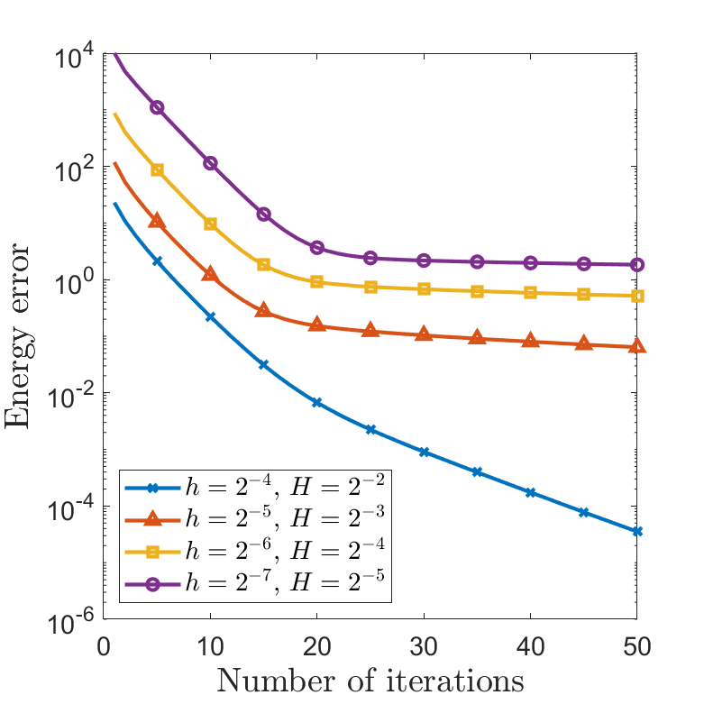
(a)

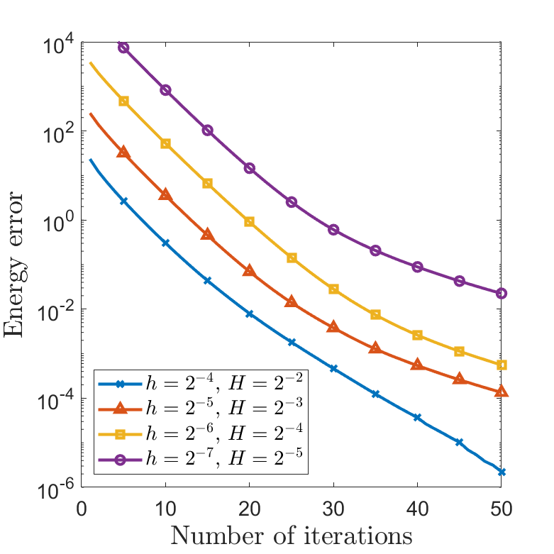
(b)

Figure 1: Decay of the relative energy error $\frac{F_{h}(u^{(n)})-F_{h}(u_{h})}{|F_{h}(u_{h})|}$ in the one- and two-level additive Schwarz methods for the displacement obstacle problem of clamped plates Eq. 3. The subdomain size $H$ and the mesh size $h$ vary satisfying $H/h=2^{2}$ and $\delta=h$.

First, we consider the displacement obstacle problem of clamped plates Eq. 3. In Eq. 1, let $f=0$ and

$$\psi(x_{1},x_{2})=-1+5|(x_{1},x_{2})-(0.5,0.5)|^{2}-|(x_{1},x_{2})-(0.5,0.5)|^{4}.$$

We note that a similar example appeared in [12, 16]. Convergence curves of the one-level additive Schwarz method are depicted in Fig. 1(a). We observe that the convergence rate of the one-level method becomes very slow when the mesh size $h$ becomes small. Such a phenomenon can be explained by Theorem 3.1; the convergence rate of the one-level method depends on $\delta^{-4}$ when $H/\delta$ is fixed. On the contrary, as shown in Fig. 1(b), the asymptotic convergence rate of the two-level method does not decrease even if $h$ becomes small. More precisely, the convergence curves for $h\leq 2^{-5}$ seem to be almost parallel to each other when the number of iterations is large enough. This verifies Theorem 4.15, which says that the convergence rate of the two-level method is uniformly bounded when the ratios $H/h$ and $H/\delta$ are fixed.

6.2 Elliptic distributed optimal control problem

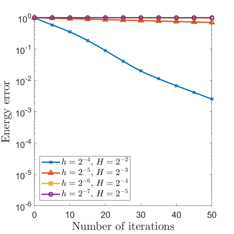
(a)

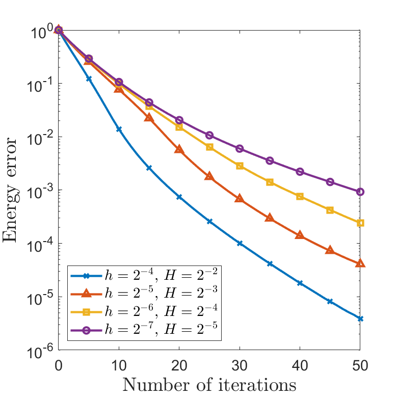
(b)

Figure 2: Decay of the relative energy error $\frac{F_{h}(u^{(n)})-F_{h}(u_{h})}{|F_{h}(u_{h})|}$ in the one- and two-level additive Schwarz methods for the elliptic distributed optimal control problem Eq. 4. The subdomain size $H$ and the mesh size $h$ vary satisfying $H/h=2^{2}$ and $\delta=h$.

Next, we deal with the elliptic distributed optimal control problem Eq. 4. We consider an example appeared in [11, 15, 30]; we set $\beta=10^{-4}$, $f(x_{1},x_{2})=\sin(4\pi x_{1}x_{2})+1.5$, and $\psi=1$. Figure 2 plots the relative energy error $\frac{F_{h}(u^{(n)})-F_{h}(u_{h})}{|F_{h}(u_{h})|}$ in the one- and two-level additive Schwarz methods, when $H$ and $h$ vary satisfying $H/h=2^{2}$ and $\delta=h$. Convergence behaviors of the methods are similar to the case of the displacement obstacle problem of clamped plates. While the convergence rate of the one-level method deteriorates severely when $h$ becomes small, the two-level method shows quite fast decay of the energy error even if $h$ is large. This verifies the effectiveness of the proposed coarse space in view of acceleration of the convergence of additive Schwarz methods.

7 Conclusion

In this paper, we provided a rigorous analysis on additive Schwarz methods for fourth-order variational equalities. We proposed a novel coarse space that makes the two-level method scalable in the sense that that convergence rate is uniformly bounded when $H/h$ and $H/\delta$ are kept constant. Our theoretical results were verified by numerical experiments conducted on two examples: the displacement obstacle problem of clamped plates and the elliptic distributed optimal control problem. As far as we know, the two-level method presented in this paper is the first scalable Schwarz method for solving fourth-order variational inequalities.

This paper leaves us several interesting topics for future research. Although Theorem 4.15 is sufficient to ensure the scalability of the proposed two-level method, we do not know whether the estimate in Theorem 4.15 is sharp or not. We expect that new mathematical tools will be needed either to prove the sharpness of Theorem 4.15 or to improve the estimate, and should be considered for future work. Meanwhile, there are a number of engineering problems that can be represented as fourth-order variational inequalities. We believe that the proposed two-level method can be effectively utilized for scientific computing and numerical study of these problems.

References

• [1] L. Badea, Convergence rate of a Schwarz multilevel method for the constrained minimization of nonquadratic functionals, SIAM J. Numer. Anal., 44 (2006), pp. 449–477.
• [2] L. Badea and R. Krause, One-and two-level Schwarz methods for variational inequalities of the second kind and their application to frictional contact, Numer. Math., 120 (2012), pp. 573–599.
• [3] L. Badea, X.-C. Tai, and J. Wang, Convergence rate analysis of a multiplicative Schwarz method for variational inequalities, SIAM J. Numer. Anal., 41 (2003), pp. 1052–1073.
• [4] L. Badea and J. Wang, An additive Schwarz method for variational inequalities, Math. Comp., 69 (2000), pp. 1341–1354.
• [5] A. Beck and M. Teboulle, A fast iterative shrinkage-thresholding algorithm for linear inverse problems, SIAM J. Imaging Sci., 2 (2009), pp. 183–202.
• [6] M. Bergounioux, K. Ito, and K. Kunisch, Primal-dual strategy for constrained optimal control problems, SIAM J. Control Optim., 37 (1999), pp. 1176–1194.
• [7] P. Bochev and R. B. Lehoucq, On the finite element solution of the pure Neumann problem, SIAM Rev., 47 (2005), pp. 50–66.
• [8] F. K. Bogner, R. L. Fox, and L. A. Schmit, The generation of inter-element-compatible stiffness and mass matrices by the use of interpolation formulas, in Proceedings of the Conference on Matrix Methods in Structural Mechanics, 1965, pp. 397–443.
• [9] S. Brenner and R. Scott, The Mathematical Theory of Finite Element Methods, Springer, New York, 2008.
• [10] S. C. Brenner, A two-level additive Schwarz preconditioner for nonconforming plate elements, Numer. Math., 72 (1996), pp. 419–447.
• [11] S. C. Brenner, C. B. Davis, and L.-Y. Sung, A partition of unity method for a class of fourth order elliptic variational inequalities, Comput. Methods Appl. Mech. Engrg., 276 (2014), pp. 612–626.
• [12] S. C. Brenner, C. B. Davis, and L.-Y. Sung, Additive Schwarz preconditioners for the obstacle problem of clamped Kirchhoff plates, Electron. Trans. Numer. Anal., 49 (2018), pp. 274–290.
• [13] S. C. Brenner, J. Gedicke, and L.-Y. Sung, ${C}^{0}$ interior penalty methods for an elliptic distributed optimal control problem on nonconvex polygonal domains with pointwise state constraints, SIAM J. Numer. Anal., 56 (2018), pp. 1758–1785.
• [14] S. C. Brenner and L.-Y. Sung, A new convergence analysis of finite element methods for elliptic distributed optimal control problems with pointwise state constraints, SIAM J. Control Optim., 55 (2017), pp. 2289–2304.
• [15] S. C. Brenner, L.-Y. Sung, and Z. Tan, A $C^{1}$ virtual element method for an elliptic distributed optimal control problem with pointwise state constraints, Math. Models Methods Appl. Sci., 31 (2021), pp. 2887–2906.
• [16] S. C. Brenner, L.-Y. Sung, and K. Wang, Additive Schwarz preconditioners for ${C}^{0}$ interior penalty methods for the obstacle problem of clamped Kirchhoff plates, Numer. Methods Partial Differential Equations, 38 (2022), pp. 102–117.
• [17] S. C. Brenner, L.-Y. Sung, and Y. Zhang, Finite element methods for the displacement obstacle problem of clamped plates, Math. Comp., 81 (2012), pp. 1247–1262.
• [18] S. C. Brenner and K. Wang, Two-level additive Schwarz preconditioners for ${C}^{0}$ interior penalty methods, Numer. Math., 102 (2005), pp. 231–255.
• [19] L. Calatroni and A. Chambolle, Backtracking strategies for accelerated descent methods with smooth composite objectives, SIAM J. Optim., 29 (2019), pp. 1772–1798.
• [20] E. Casas, Control of an elliptic problem with pointwise state constraints, SIAM J. Control Optim., 24 (1986), pp. 1309–1318.
• [21] J. Cui and Y. Zhang, A new analysis of discontinuous Galerkin methods for a fourth order variational inequality, Comput. Methods Appl. Mech. Engrg., 351 (2019), pp. 531–547.
• [22] M. Dryja and O. B. Widlund, Domain decomposition algorithms with small overlap, SIAM J. Sci. Comput., 15 (1994), pp. 604–620.
• [23] W. Gong and N. Yan, A mixed finite element scheme for optimal control problems with pointwise state constraints, J. Sci. Comput., 46 (2011), pp. 182–203.
• [24] M. Hintermüller, K. Ito, and K. Kunisch, The primal-dual active set strategy as a semismooth Newton method, SIAM J. Optim., 13 (2002), pp. 865–888.
• [25] C.-O. Lee, A nonconforming multigrid method using conforming subspaces, in The Sixth Copper Mountain Conference on Multigrid Methods, 1993, pp. 317–330.
• [26] C.-O. Lee and J. Park, Recent advances in domain decomposition methods for total variation minimization, J. Korean Soc. Ind. Appl. Math., 24 (2020), pp. 161–197.
• [27] C.-O. Lee and J. Park, A dual-primal finite element tearing and interconnecting method for nonlinear variational inequalities utilizing linear local problems, Internat. J. Numer. Methods Engrg., 122 (2021), pp. 6455–6475.
• [28] J. Lee, Two domain decomposition methods for auxiliary linear problems of a multibody elliptic variational inequality, SIAM J. Sci. Comput., 35 (2013), pp. A1350–A1375.
• [29] Y.-J. Lee and J. Park, On the linear convergence of additive Schwarz methods for the $p$-Laplacian, arXiv preprint arXiv:2210.09183, (2022).
• [30] W. Liu, W. Gong, and N. Yan, A new finite element approximation of a state-constrained optimal control problem, J. Comput. Math., 27 (2009), pp. 97–114.
• [31] J. Nečas, Direct Methods in the Theory of Elliptic Equations, Springer, Heidelberg, 2012.
• [32] R. Nochetto and L. Wahlbin, Positivity preserving finite element approximation, Math. Comp., 71 (2001), pp. 1405–1419.
• [33] B. O’Donoghue and E. Candes, Adaptive restart for accelerated gradient schemes, Found. Comput. Math., 15 (2015), pp. 715–732.
• [34] J. Park, Additive Schwarz methods for convex optimization as gradient methods, SIAM J. Numer. Anal., 58 (2020), pp. 1495–1530.
• [35] J. Park, Accelerated additive Schwarz methods for convex optimization with adpative restart, J. Sci. Comput., 89 (2021), p. Paper No. 58.
• [36] J. Park, Additive Schwarz methods for convex optimization with backtracking, Comput. Math. Appl., 113 (2022), pp. 332–344.
• [37] X.-C. Tai, Rate of convergence for some constraint decomposition methods for nonlinear variational inequalities, Numer. Math., 93 (2003), pp. 755–786.
• [38] X.-C. Tai, Nonlinear positive interpolation operators for analysis with multilevel grids, in Domain Decomposition Methods in Science and Engineering, 2005, pp. 477–484.
• [39] X.-C. Tai, B. Heimsund, and J. Xu, Rate of convergence for parallel subspace correction methods for nonlinear variational inequalities, in Domain Decomposition Methods in Science and Engineering (Lyon, 2000), 2002, pp. 127–138.
• [40] X.-C. Tai and J. Xu, Global and uniform convergence of subspace correction methods for some convex optimization problems, Math. Comp., 71 (2002), pp. 105–124.
• [41] A. Toselli and O. Widlund, Domain Decomposition Methods—Algorithms and Theory, Springer, Berlin, 2005.
• [42] J. Valdman, MATLAB implementation of C1 finite elements: Bogner–Fox–Schmit rectangle, in Parallel Processing and Applied Mathematics, 2020, pp. 256–266.
• [43] X. Zhang, Two-level Schwarz methods for the biharmonic problem discretized conforming ${C}^{1}$ elements, SIAM J. Numer. Anal., 33 (1996), pp. 555–570.