Heavy Neutral Leptons at Muon Colliders

Abstract

The future high-energy muon colliders, featuring both high energy and low background, could play a critical role in our searches for new physics. The smallness of neutrino mass is a puzzle of particle physics. Broad classes of solutions to the neutrino puzzles can be best tested by seeking the partners of SM light neutrinos, dubbed as heavy neutral leptons (HNLs), at muon colliders. We can parametrize HNLs in terms of the mass $m_{N}$ and the mixing angle with $\ell$-flavor $U_{\ell}$. In this work, we focus on the regime $m_{N}>O(100)$ GeV and study the projected sensitivities on the $|U_{\ell}|^{2}-m_{N}$ plane with the full-reconstructable HNL decay into a hadronic $W$ and a charged lepton. The projected reach in $|U_{\ell}|^{2}$ leads to the best sensitivities in the TeV realm.

1 Introduction

High energy muon colliders are exciting future opportunities that could probe 10 TeV scale and higher physics thoroughly thanks to its high center of mass energy and clean lepton collider environment Boscolo:2018ytm ; Delahaye:2019omf ; AlAli:2021let ; Black:2022cth ; Narain:2022qud ; Bose:2022obr ; Aime:2022flm ; Schulte:2022brl ; Zimmermann:2022xbv . The muon collider physics potential in the mysterious neutrino sector is yet to be understood. The Neutrino sector sources several puzzles of the Standard Model (SM), such as the origin of neutrino mass and the structure of its mixing Bilenky:1978nj ; Super-Kamiokande:1998uiq ; Super-Kamiokande:1998kpq ; SNO:2002tuh ; KamLAND:2002uet ; Bilenky:2005mx ; Bilenky:2005cp ; Gonzalez-Garcia:2007dlo ; King:2013eh ; Bilenky:2014ema ; ParticleDataGroup:2022pth . The neutrino sector can also help solve many pressing issues, such as matter-antimatter asymmetry through leptogenesis. Of the various approaches to account for the smallness of the neutrino mass and many puzzles, the seesaw mechanisms provide appealing natural explanations. In particular, heavy fermions carrying lepton numbers, singlets under the electroweak symmetry, are introduced in a large class of seesaw models Bjorken:1972am ; Minkowski:1977sc ; Sawada:1979dis ; Gell-Mann:1979vob ; Mohapatra:1979ia ; Yanagida:1980xy ; Schechter:1980gr ; Chang:1985en ; Langacker:1988ur ; Dittmar:1989yg ; Smirnov:1993af ; Strumia:2006db ; Mohapatra:2006gs ; Kersten:2007vk ; Davidson:2008bu ; Kusenko:2009up ; Dasgupta:2014ula and models of (partially) composite neutrinos Arkani-Hamed:1998wff ; Grossman:2010iq ; Chacko:2020zze ; Cox:2021lii .

We dub these heavy degrees of freedom with mass above MeV as heavy neutral leptons (HNLs) Chanowitz:1978mv ; Pilaftsis:1997jf ; Ma:1998dx ; Asaka:2005pn ; Abdullahi:2022jlv . Their mass range is broad since both low-scale, and high-scale mechanisms can be viable. HNLs can mix with the “active” neutrinos making it potential to be detected in various experimental facilities.

The HNL serves as a simplified benchmark elucidating a broad class of testable seesaw mechanisms. In more generalized considerations, the HNLs can uniquely serve as a singlet fermion portal between the SM sector and hidden sector physics. We can parametrize the HNL in terms of the mass $m_{N}$ and the squared mixing angle $|U_{\ell}|^{2}$ where $\ell$ refers to the flavor. Theoretically, one must introduce at least two HNLs to explain the mass difference. For simplicity of the phenomenological discussion, one chooses to turn on only one HNL at a time, which is assumed to dominate a given HNL’s flavor property. One can also instead assume a fully mixed HNL, which requires proper weighting of the sensitivities from various channels. HNLs have long been the target of particle physics searches via various experimental approaches. Depending on the mass range for $m_{N}$, the dominant decay channel for HNL can be distinct. For example, in the mass range of GeV to W boson mass, the HNL can not decay to an on-shell massive gauge boson, so the leading decay channel is three-body final states which can enhance its lifetime Thacker:1971hy ; Helo:2010cw . The HNL can be long-lived enough at the detector scale; hence one can exploit the displaced vertex signal to reconstruct the HNL Helo:2013esa ; Liu:2019ayx ; Maiezza:2015lza ; Batell:2016zod ; Antusch:2016vyf ; Antusch:2017hhu ; Cottin:2018kmq ; Abada:2018sfh ; Drewes:2019fou ; Bondarenko:2019tss . While for lower mixing angles and in the sub-GeV regime, HNL can be even more long-lived and be complementarily probed at far detectors using beam-dump experiments NA3:1985yvr ; WA66:1985mfx ; Gronau:1984ct ; Baranov:1992vq ; NOMAD:2001eyx ; FMMF:1994yvb ; SHiP:2015vad ; Ballett:2019bgd ; FASER:2018eoc ; Wang:2022jff such as CHARM CHARM:1985nku ; CHARMII:1994jjr , NuTeV NuTeV:1999kej , etc.

This paper studies the HNL detection on the muon collider and focuses on the mass regime $m_{N}>O(100)$ GeV. The decays into heavy gauge bosons or Higgs bosons is open. Hence HNL decays promptly once produced. The study in the mass range has been conducted on the LHC delAguila:2007qnc ; Alva:2014gxa ; Degrande:2016aje ; Accomando:2017qcs ; Pascoli:2018heg ; Fernandez-Martinez:2022gsu ; Abada:2022wvh ; Arganda:2015ija ; Ismail:2021dyp ; Dev:2013wba ; Das:2017nvm ; Das:2017pvt ; Das:2017gke ; Das:2018usr ; Das:2012ze and future lepton colliders Das:2012ze ; Banerjee:2015gca ; Blondel:2022qqo ; Mekala:2022cmm ; Chakraborty:2022pcc . We want to stress that at the muon collider, we can achieve better constraints on the $|U_{\ell}|^{2}-m_{N}$ plane, especially for the muon flavor. The first advantage of the muon collider is the clean environment compared to the hadron collider. We can easily control the background and avoid much QCD background noise. The fixed kinematics for the initial colliding muons make the events reconstruction much simpler. Furthermore, in contrast to the future proposed electron-positron colliders, muon colliders can achieve much higher center-of-mass energy (c.m.s). High Energy muon collider can run with $\sqrt{s}=3$ TeV and 10 TeV at the first step. This can greatly improve our probe of the new physics scale or the HNL mass scale. Exploiting such significant advantages, we will show that we can open a new specific region in the parameter space and push $U_{\mu}^{2}$ down to $O(10^{-7})$ at best.

The rest of this paper is as follows. In section 2, we make a brief introduction to the simple Type-I seesaw model and parametrize the HNL at the Lagrangian level. Then we present in detail the signal production considerations in section 3, the signal and background events generation section 4, and the analysis method and results in section 5. Finally, we conclude in section 6.

2 Theoretical Framework

This section briefly reviews the HNL theory framework relevant to this study. We begin with the simplest Type-I linear seesaw model. Introducing a new heavy fermion $N$, the Lagrangian is given by

$$\mathcal{L}_{\nu}\supset-\lambda_{\nu}\bar{L}\tilde{H}N-\frac{m_{N}}{2}\bar{N}^{c}N+\text{h.c.}\,,$$ (1)

where $\tilde{H}=i\sigma_{2}H^{*}$. In the flavor basis $\left\{\nu_{L},N^{c}\right\}$ the mass matrix is

$$M_{\nu}=\left(\begin{array}[]{cc}0&m_{D}\\ m_{D}&m_{N}\end{array}\right),$$ (4)

where $m_{D}=\lambda_{\nu}v/\sqrt{2}$ with the vacuum expectation value of the Higgs field $v=246\leavevmode\nobreak\$GeV. Diagonalizing the mass matrix, we get the two eigenvalues of the masses

$$m_{\nu}\equiv m_{1}\simeq\frac{m_{D}^{2}}{m_{N}}=m_{D}\sin\theta,\quad m_{2}\simeq m_{N}+\frac{m_{D}^{2}}{m_{N}}\simeq m_{N}$$ (5)

where we have assumed $m_{N}\gg m_{D}$. The mass eigenstates are the mixing of the two flavor states with mixing angle $\sin\theta=m_{D}/m_{N}$

$$\nu_{m}=\cos\theta\nu_{L}+\sin\theta N_{R}^{c}\ ,\quad\quad N_{m}=\cos\theta N_{R}-\sin\theta\nu_{L}^{c}\ .$$ (6)

Here the subscript $m$ refers to the mass eigenstate. In terms of physical mass, we can express

$$|U_{\ell}|^{2}=\sin^{2}\theta=\dfrac{m_{\nu}}{m_{N}}\ ,$$ (7)

where we have converted to the common convention $U_{\ell}$ to describe the mixing angle. For $\lambda_{\nu}$ taking $O(1)$ value, the mass of the HNL is too large to be accessible at colliders. There are more extended seesaw models incorporating lighter HNLs which can be testable. One example is the inverse seesaw model Das:2012ze ; Dias:2012xp ; Law:2013gma ; Mohapatra:1986bd ; Ma:1987zm ; Ma:2009gu ; Bazzocchi:2010dt . Both left-handed and right-handed neutrinos are introduced as $F_{L}$ and $F_{R}$, respectively. The relevant Lagrangian terms are

$$-\mathcal{L}_{\nu}\supset\lambda_{\nu}\bar{L}\tilde{H}F_{R}+M\bar{F}_{L}F_{R}+\dfrac{1}{2}\mu\bar{F_{L}^{c}}F_{L}+\text{h.c.}$$ (8)

The first two terms are the Dirac mass terms, and the third is the Majorana mass term. In the basis of $(\nu_{L},\,\,F_{R}^{c},\,\,F_{L})$, the mass matrix is given by

$$M_{\nu}=\begin{pmatrix}0&m_{D}&0\\ m_{D}&0&M\\ 0&M&\mu\end{pmatrix}$$ (9)

where again we have $m_{D}=\lambda_{\nu}v/\sqrt{2}$. Under the limit $\mu\ll m_{D}\ll M$, the three eigenvalues of masses are given by

$$m_{\nu}\approx\dfrac{m_{D}^{2}}{M}\dfrac{\mu}{M}\,\quad M_{1,2}\approx M\pm\dfrac{1}{2}\mu$$ (10)

and the mixing angle is given by

$$|U_{\ell}|^{2}=\sin^{2}\theta=\left(\dfrac{m_{D}}{M}\right)^{2}=\dfrac{m_{\nu}}{\mu}\ .$$ (11)

Since $\mu$ is a free parameter that is far smaller than the HNL mass, the mixing angle may be sizeable. Another interesting seesaw model is the linear seesaw model Wyler:1982dd ; Akhmedov:1995ip ; Akhmedov:1995vm , where we introduce extra fermion with Dirac mass $m_{\psi}$, and the mixing angle is given by

$$\sin\theta=\dfrac{m_{\nu}}{m_{\psi}}\ ,$$ (12)

The presence of $m_{\psi}$ violates the lepton number. Hence, we can treat $m_{N}$, the mass of HNL, and the squared mixing angle, $|U_{\ell}|^{2}$, as free parameters. As discussed in the introduction section, we choose to turn on one flavor each time and introduce one HNL which can be either Dirac or Majorana. Such a choice is convenient for collider phenomenology analysis, and we can focus on a specific flavor. Under the mixing angle with the SM neutrino flavor, we can write down the relevant interactions

$$\begin{split}\mathcal{L}\supset&\dfrac{gU_{\ell}}{\sqrt{2}}\left(W_{\mu}\bar{l}_{L}\gamma^{\mu}N+\text{h.c.}\right)-\dfrac{gU_{\ell}}{2\cos\theta_{w}}Z_{\mu}\left(\bar{\nu}_{L}\gamma^{\mu}N+\bar{N}\gamma^{\mu}\bar{\nu}_{L}\right)-U_{\ell}\dfrac{m_{N}}{v}h\left(\bar{\nu}_{L}N+\bar{N}\nu_{L}\right)\,\end{split}$$ (13)

where we only keep the linear term of $U_{\ell}$. The HNL couples to massive gauge bosons and Higgs bosons with the size suppressed by the mixing angle $U_{\ell}$. For $m_{N}$ above $O({\rm GeV})$ scale, the main production channel for HNL is from the on/off-shell massive gauge boson decay. The produced HNLs are fully polarized due to the mixing with SM left-handed neutrinos. We focus on the mass range $m_{N}$ larger than $O(100)$ GeV, the dominant decay channel for HNL is to on-shell massive gauge boson and Higgs boson. These are 1 to 2 processes so HNL will promptly decay after it is produced at the interaction point. For $m_{N}\gg m_{h}$, the lifetime of HNL is given by Pascoli:2018heg

$$\Gamma_{N}\approx\dfrac{g^{2}m_{N}^{3}}{32\pi^{2}m_{W}^{2}}|U_{\ell}|^{2}$$ (14)

Whether the HNL is Dirac or Majorana does not affect the production signature, only the left-handed component of HNL shows up due to mixing. However, it indeed impacts the decay pattern. As is shown in deGouvea:2021ual ; Balantekin:2018ukw ; BahaBalantekin:2018ppj , for the decay channel $N\rightarrow\nu+X$ in which X is a self-conjugate boson, one can define the following forward-backward symmetry $A_{\rm FB}$ in the rest frame of $N$

$$A_{\rm FB}\equiv\dfrac{\int_{0}^{1}\frac{d\Gamma}{d\cos\theta_{X}}d\cos\theta_{X}-\int_{-1}^{0}\frac{d\Gamma}{d\cos\theta_{X}}d\cos\theta_{X}}{\int_{0}^{1}\frac{d\Gamma}{d\cos\theta_{X}}d\cos\theta_{X}+\int_{-1}^{0}\frac{d\Gamma}{d\cos\theta_{X}}d\cos\theta_{X}}$$ (15)

For the Majorana HNL, the decay is isotropic at the leading order, and hence $A_{\rm FB}$ is vanishing. While for Dirac spinor, $A_{\rm FB}$ is non-zero due to the helicity selection. A similar case is for the charged lepton final states. For the Dirac spinor case, $N_{\ell}$ can only decay to $\ell^{-}$ with the same lepton number plus $W^{+}$. While for the Majorana spinor case, where the lepton numbers are no longer conserved, both $(\ell^{-},W^{+})$ and $(\ell^{+},W^{-})$ can appear in the final states. One can show that the sum of angular distributions will be isotropic if $N$ is Majorana fermion and non-isotopic for the Dirac HNL case. In this study, we only show the results of kinematics simulating the Dirac fermion case, and one can further optimize for the Majorana case.

3 HNL Productions at High Energy Muon Colliders

We study two benchmark future muon collider running scenarios. The 3 TeV muon collider benchmark has a 3 TeV center of mass energy and $1\leavevmode\nobreak\ \text{ab}^{-1}$ integrated luminosity. The 10 TeV muon collider benchmark has a 10 TeV center of mass energy with $10\leavevmode\nobreak\ \text{ab}^{-1}$ integrated luminosity.

We divide our simulation and analysis into the following four categories: the $\mu$-flavored and $e$-flavored HNL at $\sqrt{s}=3$ TeV and 10 TeV. Note that the $\tau$-flavored HNL results will be similar to that of the $e$-flavored HNL. We will discuss an extrapolation in the final section when we show the results. The Muon collider is advantageous for the muon-flavor HNL production, as the dominant production channel for $N_{\mu}$ is $t$-channel which avoids the $1/s$ suppression for the $s$-channel processes. While for $e$-flavored case, $N_{e}$ are mainly produced via the $s$-channel at 3 TeV and Vector Boson Fusion (VBF) processes at 10 TeV.

For the muon-flavored HNL, the Feynman diagram for the leading $t$-channel process is shown in the left panel of Figure 1. By exchanging $t$-channel $W$ boson, initial state muon pairs produce pairs of neutrinos, one of which can be $N_{\mu}$ due to mixing. At high $\sqrt{s}$, the forward scattering dominates; hence $N_{\mu}$ is emitted almost along the direction of $\mu^{-}$ while $\bar{N}_{\mu}$ comes out backward. The forward scattering dominance becomes more and more prominent for lighter and lighter HNLs.

While for $e/\tau$-flavored production, the leading $s$-channel diagrams are shown in the right panel of Figure 1. The muon pair first annihilates into an off-shell Z boson, which converts into $\nu_{e}+\bar{N}_{e}$ or $\bar{\nu}_{e}+N_{e}$, and this process is $p$-wave angular distributed. The angular distribution is more evenly distributed in contrast to the forward production dominance from the muon flavor. However, its cross-section is highly suppressed by the $s$-channel propagator. We plot the leading 2-to-2 cross section in Figure 2 for comparison.

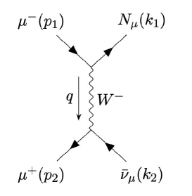
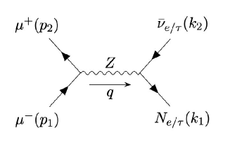
Figure 1: The Feynman diagrams for $\mu^{+}\mu^{-}\rightarrow N_{\ell}+\bar{\nu}_{\ell}$. The left panel is for $N_{\mu}$ and the right panel is for $N_{e/\tau}$.

Another important contribution to HNL production is the VBF processes. As elaborated in Han:2020uid ; AlAli:2021let , with the energy scale increased, for a fixed HNL mass, the role of the virtual electroweak gauge bosons becomes more and more relevant. The growth of the VBF rate requires a resummation of large logarithms appearing in the process. By perturbatively computing the splitting function, we can use the Parton Distribution Function (PDF) Kane:1984bb ; Dawson:1984gx ; Han:2020uid ; Fornal:2018znf ; Chen:2016wkt ; AlAli:2021let ; Costantini:2020stv to compute the scattering of these off-shell gauge bosons. Naively the cross section scales like $\alpha_{W}^{2}\log(s)$ where $\alpha_{W}=g_{W}^{2}/(4\pi)$ refers to the electroweak coupling square. Its ratio to the $s$-channel cross-section can be estimated by AlAli:2021let

$$\dfrac{\sigma_{\rm VBF}}{\sigma_{\rm s-channel}}\propto\alpha_{W}^{2}\dfrac{s}{m_{Z}^{2}}\log^{2}\dfrac{s}{m_{W}^{2}}\log\dfrac{s}{m_{N}^{2}}$$ (16)

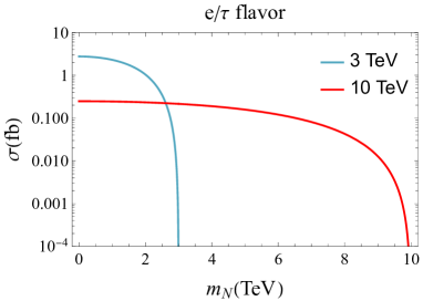
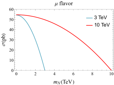
Figure 2: The cross section of the 2-to-2 process $\mu^{+}\mu^{-}\rightarrow N_{\ell}+\bar{\nu}_{\ell}$ as a function of $m_{N}$ for $\ell=\mu$ and $e$ respectively. The blue curve refers to $\sqrt{s}=3$ TeV and the red curve is for $\sqrt{s}=10$ TeV.

As the muon collider center of mass energy increases, the contribution from the VBF process can dominate over the $s$-channel process. The next section will show that, at $\sqrt{s}=3$ TeV, the cross-section of the VBF process is sub-dominant with a comparable size. While $\sqrt{s}$ reaches up to 10 TeV, the VBF process primarily contributes to the total signal rate for $e$-flavored HNL.

We used both analytical calculation, convolution with EW PDF, and event generator to study and cross-check the signal rates. We simulate the whole process using MadGraph5_aMC$@$NLO Alwall:2014hca ; Ruiz:2021tdt to generate the signal events. The Universal FeynRules Output (UFO) Degrande:2011ua models HeavyN Alva:2014gxa ; Degrande:2016aje ; Atre:2009rg generated by FeynRules Degrande:2011ua ; Alloul:2013bka is employed. The charged current decay of HNL is the focus of this study due to enhanced observability through the charged leptons and the possibility of reconstructing HNL resonance from the hadronic $W$ decays. The branching fraction of HNL decaying into this channel is shown in Figure 3 as a function of $m_{N}$. The branching fraction is independent of $|U_{\ell}|^{2}$ to the leading order. The backgrounds will be dominantly from various SM processes with hadronic $W$ bosons and as well hadronic $Z$ bosons. The next section presents the pre-selection of the signal and background events for the four categories.

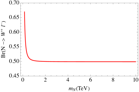
Figure 3: The branching ratio of the Dirac HNL decay channel $N_{\ell}\longrightarrow W^{+}\ell^{-}$ as a function of $m_{N}$. This channel allows full reconstruction of the HNL decay and reaches the equivalence limit of 50% at $\sim 1$ TeV.

4 Signal and Background after Pre-Selection Cuts

This section discusses the baseline signal and background cross-sections after the pre-selection cuts (PSC). As we shall see later, pre-selection cuts are sometimes needed for a consistent definition of the cross-section. PSC can help identify backgrounds that can fake the signal with particles along the beampipe or the shielding region. Also, it can help physically regular a few singularities we could encounter. We will elaborate in a later part of this section. We list all possible production channels for the signal, including the leading 2-to-2 and 2-to-4 (VBF) channels. As mentioned above, the final states considered are hadronic weak-boson jets plus a charged lepton. We assume the $W$ and $Z$ boson can be constructed by the dijets or merged fat jet system, with a conservative assumption that we cannot distinguish between hadronic $W$ and hadronic $Z$. Consequently, for signal we first consider the chanel $\mu^{+}\mu^{-}\rightarrow\bar{\nu}_{\ell}+N_{\ell}$, followed by $N_{\ell}\rightarrow\ell^{-}+W^{+}$. For background, we generate $\mu^{+}\mu^{-}\rightarrow V+\ell^{-}+X$ in which $V$ refers to either $W$ or $Z$ gauge boson, and $X$ refers to other particles escaped detection. In what follows, we discuss them channel by channel.

Several subtle points in the computation of the VBF processes are worth mentioning. First, the emitted virtual photon from the incoming muon has infrared divergence. Such divergence can be avoided using the equivalent photon approximation (EPA) or the photon PDF. The simple EPA needs to be replaced by consistent electroweak (EW) treatment at high energy muon colliders Han:2020uid . In principle, inclusive VBF processes are more conveniently calculated using PDFs of EW gauge bosons. However, when we compute the partonic cross section of the gauge bosons scattering, $t$-channel singularities arise as PDF assumes the “incoming” gauge bosons are on-shell, while in reality, they should be having space-like-separations of off-shell momentum. In other words, we encounter a fake singular behavior caused by the quasi-real partonic assumption. We will analyze the individual channel carefully and extract the primary contribution to avoid such an unphysical issue. Another interesting issue that we plan to elaborate more in future work arises. Some of the processes can be seen as the scattering of the decay debris of muon with the other anti-muon. So in the 2-to-4 diagrams, we encounter the on-shell internal propagator, which is the so-called $t$-channel singularity Ginzburg:1995bc ; Dams:2002uy ; Melnikov:1996iu . It is claimed that the cross section of such diagrams is proportional to the incoming muon beam size, so it is not a concern for us. We will elaborate in the following when we deal with the explicit diagrams.

Since the final states are composed of charged lepton, neutral lepton, and gauge bosons, we define the pre-selection cuts (PSC) on the charged lepton to be visible as follows:

$$p_{T}(\ell)>20\leavevmode\nobreak\ \text{GeV},\quad|\eta(\ell)|<2.5$$ (17)

In the following subsections, we list the cross section of various channel processes. It should be emphasized that we only enumerate the $N_{\ell}$ production, and the $\bar{N}_{\ell}$ production is the charge conjugate process of that for $N_{\ell}$. The same cases apply to the background events. We double its rate and the values in the rate columns have included both the positive charge and minus charge cases.

4.1 $\mu$-flavored HNL at 3 TeV

We list the signal cross section for various channels in Table 1. The mass $m_{N}$ is set as 1 TeV as a benchmark value. The value of the cross-section $\sigma/|U_{\ell}|^{2}$ is after $N_{\ell}$ decaying into $W^{+}+\ell^{-}$ and a pre-selection cut on $\ell^{-}$ discussed earlier. The first row shows the result of the leading 2-to-2 $t$-channel process, which is over 40 pb. The bottom rows are for the VBF channels where the muon pair in the final states are made invisible. As we can see, the signal rate of the leading $t$-channel process is at least two orders larger in magnitude than that of the 2-to-4 VBF processes. Hence we only keep the 2-body process to when considering the muon-flavored HNL.

Type	Signal process	$\sigma/|U_{\mu}|^{2}$ (w. conj. channel) $m_{N}=1\leavevmode\nobreak\ \text{TeV}$	Pre-selection cut (PSC)	Included
$t$-channel	$\mu^{+}\mu^{-}\longrightarrow N_{\mu}\bar{\nu}_{\mu}$	43.5 pb	PSC	Yes
VBF	$\mu^{+}\mu^{-}\longrightarrow\mu^{+}\mu^{-}N_{\mu}\bar{\nu}_{\mu}$	$\sim 1$ pb	–	No
VBF	$\mu^{+}\mu^{-}\longrightarrow\bar{\nu}_{\mu}\nu_{\mu}N_{\mu}\bar{\nu}_{\mu}$	$\sim 0.1$ pb	–	No

Table 1: The signal rate for $N_{\mu}$ at 3 TeV muon collider. The pre-selection cut is defined as: $p_{T}(\ell^{-})>20\leavevmode\nobreak\ \text{GeV}$ and $|\eta(\ell^{-})|<2.5$ where $\ell^{-}$ comes from $N_{\ell}$ decay. The cross-section includes the charge conjugate process.

Various channels for the background events are listed in Table 2. The primary channels are $\mu^{+}\mu^{-}\longrightarrow W^{+}\mu^{-}\bar{\nu}_{\mu}$ with $\sigma\sim 0.8$ pb and $\mu^{+}\mu^{-}\longrightarrow Z\mu^{+}\mu^{-}$ with $\sigma\sim 0.6$ pb. The sub-leading VBF processes are listed in the bottom lines, and we will analyze them in detail next.

The cross-sections of each background process are shown below. The pre-selection cut is defined as: $p_{T}(\mu^{-})>20\leavevmode\nobreak\ \text{GeV},|\eta(\mu^{-})|<2.5$

Type	Background process	$\sigma$ (w. conj. channel)	Pre-selection cut (PSC)	Included
$t$-channel	$\mu^{+}\mu^{-}\longrightarrow W^{+}\mu^{-}\bar{\nu}_{\mu}$	0.788 pb	PSC	Yes
$t$-channel	$\mu^{+}\mu^{-}\longrightarrow Z\mu^{+}\mu^{-}$	$0.62$ pb	PSC & missing $\mu^{+}$	Yes
VBF	$\mu^{+}\mu^{-}\longrightarrow\mu^{+}\mu^{-}W^{+}\mu^{-}\bar{\nu}_{\mu}$	$0.18$ pb	PSC & missing $\mu^{+}\mu^{-}$	Yes
VBF	$\mu^{+}\mu^{-}\longrightarrow\bar{\nu}_{\mu}\nu_{\mu}W^{+}\mu^{-}\bar{\nu}_{\mu}$	$0.028$ pb	PSC	Yes
VBF	$\mu^{+}\mu^{-}\longrightarrow\bar{\nu}_{e}\nu_{e}W^{+}\mu^{-}\bar{\nu}_{\mu}$	$0.004$ pb	PSC	No

Table 2: $N_{\mu}$ background at 3 TeV. The cross section includes the charge conjugate process.

For the first VBF process $\mu^{+}\mu^{-}\longrightarrow\mu^{+}\mu^{-}W^{+}\mu^{-}\bar{\nu}_{\mu}$, the major contribution is from the virtual photon emitted from the muon, namely from the following two partonic subprocesses:

$$\gamma^{*}\gamma^{*} \longrightarrow W^{+}W^{-},\quad W^{-}\longrightarrow\mu^{-}\bar{\nu}_{\mu}$$

$$Z^{*}\gamma^{*} \longrightarrow W^{+}W^{-},\quad W^{-}\longrightarrow\mu^{-}\bar{\nu}_{\mu}\ .$$

We extract the leading contribution, namely the pair of $\mu^{-}\bar{\nu}_{\mu}$ from the on-shell decay of $W^{-}$ boson. Other diagrams with off-shell propagators will be suppressed. For the $Z^{*}$ initial state, if we choose to generate $Z\gamma\rightarrow W^{+}\mu^{-}\bar{\nu}_{\mu}$, we will encounter diagrams with the on-shell internal muon propagator, the unphysical $t$-channel singularity. As we can see in the 2-to-5 process reported, this diagram is suppressed and can be ignored. We can focus on the two produced on-shell $W$ bosons followed by the decay of $W^{-}$.

For the second VBF process, $\mu^{+}\mu^{-}\longrightarrow\bar{\nu}_{\mu}\nu_{\mu}W^{+}\mu^{-}\bar{\nu}_{\mu}$, it is dominated by the PDF of W boson. Here we need to make sure $\mu^{-}$ is visible, which ensures that the photon PDF does not contribute significantly and there is no singularity for this channel. To avoid fake singularity when using $W$ boson PDF, we choose to run the full 2-to-5 process. Its cross-section is around 15% of the first VBF processes with exchanging photons. This is consistent with our physics intuition since the photon PDF dominates over the massive gauge bosons. The last VBF process is far more suppressed because $\bar{\nu}_{e}\nu_{e}$ pair is mainly from an on-shell $Z$ boson, and the VBF processes are suppressed due to the pre-selection cuts on $\mu^{-}$. We elect to ignore this channel due to its tiny contribution.

4.2 $\mu$-flavored HNL at 10 TeV

Here we list the cross section in Table 3 and Table 4 for signal and background channels on 10 TeV muon collider. The strategy is similar to the 3 TeV case discussed earlier.

Type	Signal process	$\sigma/|U_{\mu}|^{2}$ (w. conj. channel) $m_{N}=1\leavevmode\nobreak\ \text{TeV}$	Pre-selection cut (PSC)	Included
$t$-channel	$\mu^{+}\mu^{-}\longrightarrow N_{\mu}\bar{\nu}_{\mu}$	20.28 pb	PSC	Yes
VBF	$\mu^{+}\mu^{-}\longrightarrow\mu^{+}\mu^{-}N_{\mu}\bar{\nu}_{\mu}$	$\sim 1$ pb	–	No
VBF	$\mu^{+}\mu^{-}\longrightarrow\bar{\nu}_{\mu}\nu_{\mu}N_{\mu}\bar{\nu}_{\mu}$	$\sim 0.1$ pb	–	No

Table 3: The signal rate for $N_{\mu}$ at 10 TeV. The cross section includes the charge conjugate process.

We ignore the VBF processes for signal only to keep the leading $t$-channel diagram. The signal rate before pre-selection cuts increases slightly compared to that on 3 TeV.

For background events, the cross-section of the $t$-channel processes is reduced compared to 3 TeV. This is because most of the forwarding events are rejected by the PSC. The cross-section of VBF processes is increased by at least a factor of 2. The gauge boson PDF will be enhanced as $\sqrt{s}$ jumps from 3 TeV to 10 TeV. On the other hand, the final state particles are more boosted, leading to fewer events passing the pre-selection cuts. As a result, the VBF process is comparable in size to that of 2-to-3 $t$-channel processes.

Type	Background process	$\sigma$ (w. conj. channel)	Pre-selection cut (PSC)	Included
$t$-channel	$\mu^{+}\mu^{-}\longrightarrow W^{+}\mu^{-}\bar{\nu}_{\mu}$	0.214 pb	PSC	Yes
$t$-channel	$\mu^{+}\mu^{-}\longrightarrow Z\mu^{+}\mu^{-}$	$0.464$ pb	PSC & missing $\mu^{+}$	Yes
VBF	$\mu^{+}\mu^{-}\longrightarrow\mu^{+}\mu^{-}W^{+}\mu^{-}\bar{\nu}_{\mu}$	$0.401$ pb	PSC & missing $\mu^{+}\mu^{-}$	Yes
VBF	$\mu^{+}\mu^{-}\longrightarrow\bar{\nu}_{\mu}\nu_{\mu}W^{+}\mu^{-}\bar{\nu}_{\mu}$	$0.0686$ pb	PSC	No

Table 4: $N_{\mu}$ background at 10 TeV. The cross section includes the charge conjugate process.

4.3 $e$-flavored HNL at 3 TeV

Compared to the $\mu$-flavored case, there is no $t$-channel enhancement for the $e$-flavored case. The leading 2-to-2 channel is via exchanging $Z$ boson in $s$-channel. Hence its signal rate scales like $s^{-1}$. The leading VBF processes are similar to the $\mu$-flavored case, except that the $N_{e}$ cannot be emitted directly from the muon.

Type	Signal process	$\sigma/|U_{e}|^{2}$ (w. conj. channel)		Pre-selection (PSC)	Included
		$m_{N}=1\leavevmode\nobreak\$TeV	$m_{N}=2.5\leavevmode\nobreak\$TeV
$s$-channel	$\mu^{+}\mu^{-}\longrightarrow N_{e}\bar{\nu}_{e}$	0.0024 pb	0.00036 pb	PSC	Yes
VBF	$\mu^{+}\mu^{-}\longrightarrow\bar{\nu}_{\mu}\nu_{\mu}N_{e}\bar{\nu}_{e}$	$0.0008$ pb	$9.2\times 10^{-6}$ pb	PSC	Yes
VBF	$\mu^{+}\mu^{-}\longrightarrow\mu^{+}\mu^{-}N_{e}\bar{\nu}_{e}$	$3.1\times 10^{-5}$ pb	$\sim 10^{-8}$ pb	–	No

Table 5: The signal rate for $N_{e}$ at 3 TeV muon collider. The pre-selection cut is defined as: $p_{T}(\ell^{-})>20\leavevmode\nobreak\ \text{GeV}$ and $|\eta(\ell^{-})|<2.5$ where $\ell^{-}$ comes from $N_{\ell}$. The cross section includes the charge conjugate process.

For the second VBF process $\mu^{+}\mu^{-}\longrightarrow\mu^{+}\mu^{-}N_{e}\bar{\nu}_{e}$, a pair of (virtual) photons cannot convert to a pair of neutrinos at tree-level. The cross section of a single photon scatters with an incoming muon is suppressed. We choose to run the full 2-to-4 VBF processes instead of using gauge boson PDF since there is no divergence.

Type	Background process	$\sigma$(w. conj. channel)	Pre-selection (PSC)	Included
$t$-channel	$\mu^{+}\mu^{-}\longrightarrow W^{+}e^{-}\bar{\nu}_{e}$	0.034 pb	PSC	Yes
$t$-channel	$\mu^{+}\mu^{-}\longrightarrow Ze^{+}e^{-}$	$0.014$ pb	PSC & missing $e^{+}$	No
VBF	$\mu^{+}\mu^{-}\longrightarrow\mu^{+}\mu^{-}W^{+}e^{-}\bar{\nu}_{e}$	$0.162$ pb	PSC & missing $\mu^{+}\mu^{-}$	Yes
VBF	$\mu^{+}\mu^{-}\longrightarrow\mu^{-}\bar{\nu}_{\mu}W^{+}e^{-}e^{+}$	$0.070$ pb	PSC & missing $\mu^{-}e^{+}$	Yes
VBF	$\mu^{+}\mu^{-}\longrightarrow\bar{\nu}_{\mu}\nu_{\mu}W^{+}e^{-}\bar{\nu}_{e}$	$0.024$ pb	PSC	Yes

Table 6: $N_{e}$ background at 3 TeV. The final results include the conjugate process that doubles the cross-section reported here.

For the background, extra care is needed. The first $t$-channel is $\mu^{+}\mu^{-}\longrightarrow W^{+}e^{-}\bar{\nu}_{e}$ which is the known channel with $t$-channel singularity. As we discussed earlier, we can ignore this divergence due to the small beam size. The primary contribution is extracted through,

$$\mu^{+}\mu^{-}\longrightarrow W^{+}W^{-},\quad W^{-}\longrightarrow e^{-}\bar{\nu}_{e}$$ (18)

For the second $t$-channel process, the main diagram is

$$\mu^{+}\mu^{-}\longrightarrow ZZ,\quad Z\longrightarrow e^{-}\bar{\nu}_{e}$$ (19)

For the first VBF process $\mu^{+}\mu^{-}\longrightarrow\mu^{+}\mu^{-}W^{+}e^{-}\bar{\nu}_{e}$, the dominant contribution is from the photon PDF. It turns out this subprocess takes the largest part of the background. We have

$$\gamma^{*}\gamma^{*}\longrightarrow W^{+}W^{-},\quad W^{-}\longrightarrow e^{-}\bar{\nu}_{e}$$ (20)

The second largest VBF process is on the second last row, $\mu^{+}\mu^{-}\longrightarrow\mu^{-}\bar{\nu}_{\mu}W^{+}e^{-}e^{+}$. The primary contribution is from the scattering of the virtual photon and $\mu^{+}$. The $t$-channel singularity shows up in $\gamma^{*}\mu^{+}\longrightarrow\bar{\nu}_{\mu}W^{+}e^{-}e^{+}$ due to the subprocess $\gamma^{*}\nu_{e}\longrightarrow W^{+}e^{-}$ where $\nu_{e}$ is the on-shell decay product from $\mu^{+}$. Hence we generate the following

$$\gamma^{*}\mu^{+}\longrightarrow\bar{\nu}_{\mu}W^{+}Z,\quad Z\longrightarrow e^{+}e^{-}$$ (21)

A similar singularity would appear for the last VBF process. We can divide it into the following two channels:

$$\begin{split}&\mu^{+}\mu^{-}\longrightarrow\bar{\nu}_{\mu}\nu_{\mu}W^{+}W^{-},\quad W^{-}\longrightarrow e^{-}\bar{\nu}_{e}\\ &\mu^{+}\mu^{-}\longrightarrow ZW^{+}W^{-},\quad Z\longrightarrow\bar{\nu}_{\mu}\nu_{\mu},\quad W^{-}\longrightarrow e^{-}\bar{\nu}_{e}\end{split}$$ (22)

4.4 $e$-flavored HNL at 10 TeV

The cross sections for $e$-flavored signal processes at 10 TeV muon collider are listed in Table 7. As can be seen, the cross-section drops with increasing $m_{N}$. The VBF process dominates at low $m_{N}$, and drops quickly in the high $m_{N}$ regime due to the PDF suppression.

Type	Signal process	$\sigma/|U_{e}|^{2}$ (w. conj. channel)		Pre-selection (PSC)	Included
		$m_{N}=1\leavevmode\nobreak\$TeV	$m_{N}=9\leavevmode\nobreak\$TeV
$s$-channel	$\mu^{+}\mu^{-}\longrightarrow N_{e}\bar{\nu}_{e}$	0.00024 pb	$1.3\times 10^{-5}$ pb	PSC	Yes
VBF	$\mu^{+}\mu^{-}\longrightarrow\bar{\nu}_{\mu}\nu_{\mu}N_{e}\bar{\nu}_{e}$	$0.0046$ pb	$5.2\times 10^{-6}$ pb	PSC	Yes
VBF	$\mu^{+}\mu^{-}\longrightarrow\bar{\nu}_{e}\nu_{e}N_{e}\bar{\nu}_{e}$	$6.0\times 10^{-6}$ pb	$\sim 10^{-9}$ pb	–	No
VBF	$\mu^{+}\mu^{-}\longrightarrow\mu^{+}\mu^{-}N_{e}\bar{\nu}_{e}$	$0.00028$ pb	$6.8\times 10^{-8}$ pb	PSC & missing $\mu^{+}\mu^{-}$	Yes

Table 7: The signal rate for $N_{e}$ at 10 TeV muon collider. The cross section includes the charge conjugate process.

For 10 TeV $e$-flavored HNL background, the process of $\mu^{+}\mu^{-}\longrightarrow\bar{\nu}_{\mu}\nu_{\mu}W^{+}e^{-}\bar{\nu}_{e}$ is negligible comparing to other two VBF processes. As we will see in the next section, after the analysis cuts, $t$-channel is the dominant background for high-$m_{N}$ regions, and the other two VBF processes dominate in the middle/low-$m_{N}$ regions.

Type	Background process	$\sigma$ (w. conj. channel)	Pre-selection (PSC)	Included
$t$-channel	$\mu^{+}\mu^{-}\longrightarrow W^{+}e^{-}\bar{\nu}_{e}$	0.030 pb	PSC	Yes
$t$-channel	$\mu^{+}\mu^{-}\longrightarrow Ze^{+}e^{-}$	$0.00010$ pb	PSC missing $e^{+}$	No
VBF	$\mu^{+}\mu^{-}\longrightarrow\mu^{+}\mu^{-}W^{+}e^{-}\bar{\nu}_{e}$	$0.40$ pb	PSC & missing $\mu^{-}\mu^{+}$	Yes
VBF	$\mu^{+}\mu^{-}\longrightarrow\bar{\nu}_{\mu}\nu_{\mu}W^{+}e^{-}\bar{\nu}_{e}$	$0.063$ pb	PSC	No
VBF	$\mu^{+}\mu^{-}\longrightarrow\mu^{-}\bar{\nu}_{\mu}W^{+}e^{-}e^{+}$	$0.22$ pb	PSC missing $\mu^{-}e^{+}$	Yes

Table 8: $N_{e}$ background at 10 TeV. The cross section includes the charge conjugate process.

5 Analysis

After generating the signal and background events passing the pre-selection cuts in the previous section, we proceed with the analysis and report in this section. The heavy neutrino mass $m_{N}$ can be reconstructed through the invariant mass of the hadronic $W$ and $\ell$ (charged lepton) system. We impose mass-window cut on $m_{N}$ and generally consider the transverse momentum $p_{T}$, pseudorapidity $\eta$, and energy $E$ of the charged lepton $\ell$ and hadronic weak boson. Selection cuts are chosen to enable a high signal-background ratio while conservatively not too narrow to allow for unaccounted experimental effects. These considerations enable us to derive realistic projections on muon collider physics potential on HNLs.

5.1 $\mu$-flavored HNL at 3 TeV

The cuts we have made step by step are listed in the following:

1. Pre-selection cuts: Only one charged lepton in the final state, satisfying $|\eta(\ell)|<2.5,p_{T}(\ell)>20\leavevmode\nobreak\ \text{GeV}$ and veto additional charged leptons.

2. Central hadronic $W$ selection: $|\eta(W)|<2.5,p_{T}(W)>20\leavevmode\nobreak\ \text{GeV}$, since the forward hadronic W are not detectable (or detectable but have poor resolution and low efficiency).

3. Mass window: The HNL is reconstructed from the combination of $\ell$ and hadronic $W$. The invariant mass $m_{W\ell}$ is peaked around the $m_{N}$ value for the signal. Due to finite mass resolution, the mass windows for all benchmarks are set as $m_{N}\pm 5\%m_{N}$.

4. Optimization cuts: Customized missing $p_{T}$ for each $m_{N}$ and $E(W)<1450\leavevmode\nobreak\ \text{GeV}$.

Process	Central $W$	Mass window 150/500/1500/2500 GeV	Optimization
Background	59.15%	0.63/2.5/2.2/1.3%	0.31/0.90/0.95/0.62%
$m_{N}=150$ GeV	22.09%	22.09%	21.80%
$m_{N}=500$ GeV	91.20%	91.20%	77.59%
$m_{N}=1500$ GeV	99.87%	99.87%	89.79%
$m_{N}=2500$ GeV	99.96%	99.96%	92.09%

Table 9: Cutflow table for $N_{\mu}$ at 3 TeV. All processes after pre-selection are set to 100%. The cutflow table for individual background channels is shown in the appendix in Table 14.

We summarize the selection efficiencies after the central $W$ cut, the mass window imposition, and the optimization cuts in Table 9. Starting from the pre-selection events, we calculate the remaining fraction for each step. For low $m_{N}$, the central $W$ rejects a sizable fraction of the signal events. This low efficiency is caused by the $t$-channel forward and boosted HNL decays into forward $W$s. For higher $m_{N}$ values, these cuts keep over 90% signal events. After the mass window cut, the background events are reduced to O(1%). The optimization can further reject at least half of the background events.

After applying pre-selection, central $W$, and mass-window cuts, the missing $p_{T}$ cut is implemented. The distribution of missing $p_{T}$ for four selective $m_{N}$ benchmark values are shown in the first column of Figure 4. The red normalized distributions represent the signal events, and the blue represents the background events. For example, we can put a lower cut on $\not{p}_{T}=200$ GeV for $m_{N}=150\leavevmode\nobreak\ \text{GeV}$ to reject the majority of background events while keeping most of the signal events. For higher $m_{N}$ values, the signal distribution moves to the lower $\not{p}_{T}$ regime. We can maintain most of the signal events in such cases by imposing an upper cut on $\not{p}_{T}$. For example, we implement the cut $\not{p}_{T}<200$ GeV for $m_{N}=1500$ GeV.

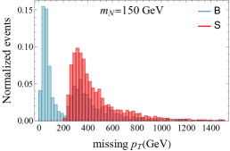
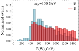
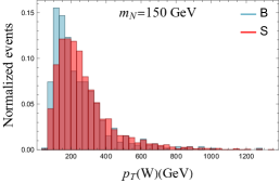
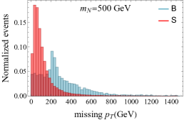
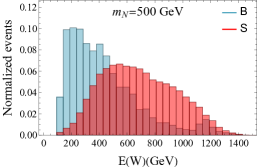
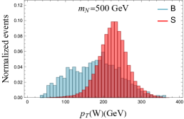
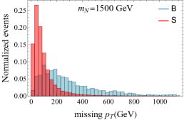
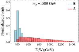
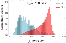
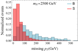
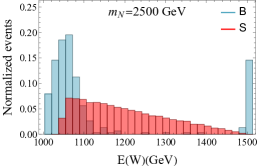
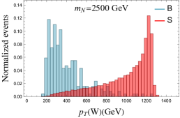
Figure 4: The normalized signal and background distributions $\mu$-flavored HNL at 3 TeV. The left column refers to the missing $p_{T}$ distribution after pre-selection and central $W$ cut. The middle column refers to $E(W)$ distribution after missing $p_{T}$ cuts. The right column refers to $p_{T}(W)$ distribution after $E(W)$ cut. Blue and red bins represent background and signal distributions, respectively.

Furthermore, we put a small cut on $E(W)<1450\leavevmode\nobreak\ \text{GeV}$. A majority background events are from $\mu^{+}\mu^{-}\longrightarrow W^{+}W^{-},W^{-}\longrightarrow\mu^{-}\bar{\nu}_{\mu}$ in which the on-shell $W$ boson carries the energy $E(W^{+})=\sqrt{s}/2$. As shown in the middle column of Figure 4, in the high-mass regions, the background events tend to accumulate at 1500 GeV. For the low-mass region, there is no such pattern, but such a small cut does not affect the background and signal. Generally, both $E(W)$ and $p_{T}(W)$ provide more distinguishing power in the high-mass region. After imposing one of the above two variables, the distribution of the other variable becomes less distinctive between signal and background. However, the background accumulation at 1500 GeV only appears in $E(W)$ distribution and can be rejected by a light cut on $E(W)$. Therefore, we choose $p_{T}(W)$ as the final variable to improve the sensitivity after $E(W)<1450$ GeV.

After the optimization cuts, the background and signal can be well separated by the distribution of W boson’s $p_{T}$, especially in the high-mass regions. As shown on the right column of Figure 4, the peak value of $p_{T}(W)$ stays at around 200 GeV, while the peak for signal shifts to higher $p_{T}$ regime as $m_{N}$ increases.

Considering the difference between background and signal distribution, we compute the significance by breaking the $p_{T}(W)$ distribution into 20 bins: $s=\sqrt{\sum S_{i}^{2}/B_{i}}$. The exclusion limit of $|U|^{2}$ is calculated under 95% CL ($s<1.96$).

5.2 $\mu$-flavored HNL at 10 TeV

The analysis for $\mu$-flavored case at 10 TeV is the same as 3 TeV. After pre-selection, central $W$ and mass-window cuts, the customized cut on missing $p_{T}$, and a small cut on $E(W)$ are implemented. We replaced the cut $E(W)<1450$ GeV with $E(W)<4950$ GeV. The calculation of significance is changed from 20 bins to 2 bins due to low statistics. The cutflow table is shown in Table 10.

Process	Central $W$	Mass window 150/1000/5000/9000 GeV	Optimization
Background	34.33%	0.65/0.79/0.66/0.33%	0.057/0.37/0.22/0.16%
$m_{N}=150$ GeV	55.04%	55.04%	55.04%
$m_{N}=1000$ GeV	54.75%	54.75%	51.63%
$m_{N}=5000$ GeV	99.93%	99.93%	97.46%
$m_{N}=9000$ GeV	99.99%	99.99%	98.27%

Table 10: Cutflow table for $N_{\mu}$ at 10 TeV. All processes after pre-selection are set to 100%.

After pre-selection, central $W$, and mass-window cuts, the optimization cut is implemented on missing transverse momentum $\not{p}_{T}$. The events concentrated at low $\not{p}_{T}$ refer to VBF background. Those spread on higher $\not{p}_{T}$ belong to the non-VBF background as shown in Figure 5. For $m_{N}=150$ GeV, we only retain those events with $\not{p}_{T}<$ 500 GeV. While for higher mass values, we reject the higher $\not{p}_{T}$ events. The cut is conducted on $\not{p}_{T}=$ 500, 400, and 250 GeV for $m_{N}$ equal to 1000, 1500, and 2500 GeV, respectively.

After applying the cut of missing $p_{T}$, we add a small cut on $E(W)<4950\leavevmode\nobreak\ \text{GeV}$. As shown in the middle column of Figure 5, in the high-mass region, the background events tend to accumulate at 5000 GeV. For the low-mass regions, there is no such pattern, but this small cut does not affect the background and signal. For the same reason, in the 3 TeV case, we prefer to leave the cut space for $p_{T}(W)$, which separates the background better. The $p_{T}(W)$ distribution is used to compute the significance.

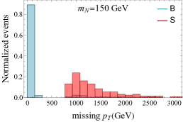
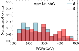
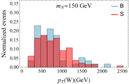
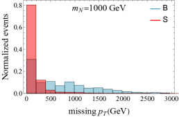
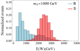
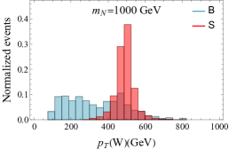
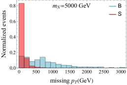
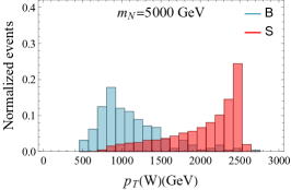
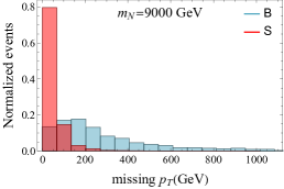
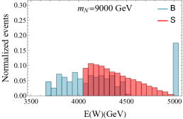
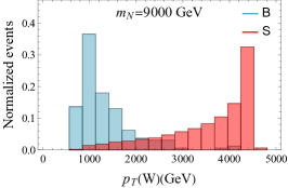
Figure 5: The normalized signal and background distributions of $\mu$-flavored HNL at 10 TeV. The left column refers to the missing $p_{T}$ distribution after pre-selection and central $W$ cut. The middle column refers to $E(W)$ distribution after missing $p_{T}$ cuts. The right column refers to $p_{T}(W)$ distribution after $E(W)$ cut. Blue and red bins represent background and signal distributions, respectively.

5.3 $e$-flavored HNL at 3 TeV

The analysis of $e$-flavored HNL at 3 TeV follows $\mu$-flavored analysis. Importantly, the missing $p_{T}$ distributions differ from the $\mu$-flavored signal. Considering the $\mu$-flavored signal, $t$-channel prefers a forward scattering (low $p_{T}(\nu)$), and such preference causes a skewed distribution for missing $p_{T}$, which is the same as the background. However, the $s$-channel is a main part of the $e$-flavored signal, which exhibits an opposite shape. The missing $p_{T}$ for both channels under $m_{N}=1000\leavevmode\nobreak\ \text{GeV}$ is shown in Figure 6. Therefore, a cut on missing $p_{T}$ is expected to reduce the background effectively.

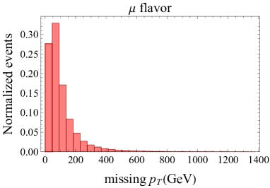
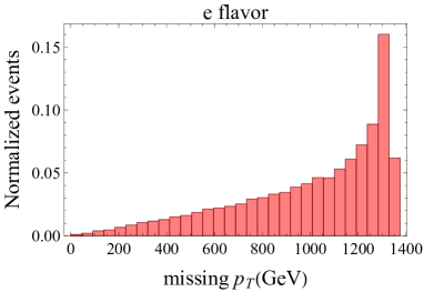
Figure 6: The missing $p_{T}$ distribution for the leading $\mu^{+}\mu^{-}\longrightarrow N_{\ell}+\bar{\nu}_{\ell}$ process at $\sqrt{s}=3$ TeV. The left panel is for $\mu$-flavored signal ($t$-channel), and the right is for $e$-flavored signal ($s$-channel).

The cutflow process followed as $\mu$ case. We take the same pre-selection cuts, central hadronic $W$ selection, and the mass window cut on $m_{W\ell}$ as in the $\mu$-flavored case. For the optimization cuts, we impose a cut of $E(W)<1450$ GeV, and the customized $\not{p}_{T}$ cuts for each $m_{N}$ benchmark.

Process	Central $W$	Mass window 150/500/1500/2500 GeV	Optimization
Background	61.96%	1.8/2.2/0.54/2.2%	0.066/0.016/0.035/0.051%
$m_{N}=150$ GeV	94.52%	94.52%	70.22%
$m_{N}=500$ GeV	97.33%	97.33%	65.13%
$m_{N}=1500$ GeV	98.92%	98.92%	77.58%
$m_{N}=2500$ GeV	98.98%	98.98%	67.45%

Table 11: Cutflow table for $N_{e}$ at 3 TeV. All processes after pre-selection are set to 100%.

We summarize the selection efficiencies under each cut in Table 11. After the mass window cuts, only $O(1)\%$ of the background events are maintained, and this ratio can be reduced to $O(0.01)\%$ after the optimization cuts.

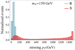
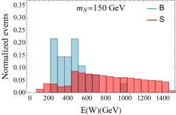
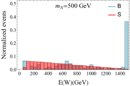
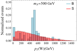
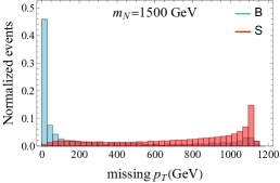
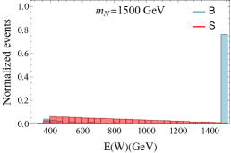
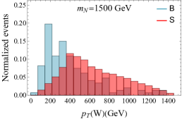
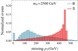
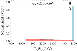
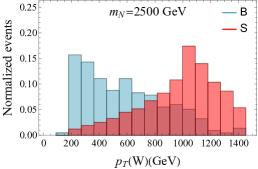
Figure 7: The normalized signal and background distributions $e$-flavored HNL at 3 TeV. The left column refers to the missing $p_{T}$ distribution after pre-selection and central $W$ cut. The middle column refers to $E(W)$ distribution after missing $p_{T}$ cuts. The right column refers to $p_{T}(W)$ distribution after $E(W)$ cut. Blue and red bins represent background and signal distributions, respectively.

After the mass window cuts, the $\not{p}_{T}$ distributions are shown on the first column of Figure 7. For low $m_{N}$ cases, we can see two peaks for the signal shape. The part of signal events that accumulate on the right is from the 2-to-2 $t$-channel process, while the events peaked at low missing $p_{T}$ regime are from the VBF processes. Since the VBF events are mostly concentrated at low $\sqrt{\hat{s}}$ region, as the value of $m_{N}$ increases, the VBF contribution to the signal is gradually diminishing. For the background, the dominant channel is $\gamma^{*}\gamma^{*}\longrightarrow W^{+}W^{-},\,W^{-}\longrightarrow\mu^{-}\bar{\nu}_{e}$ which leads to the highly forward $\bar{\nu}_{e}$. Therefore the background peaks at low $\not{p}_{T}$ region. This feature allows us to select the events at higher $\not{p}_{T}$.

We show the distribution of $E(W)$ and $p_{T}(W)$ again in the middle and right columns of Figure 7. For a similar reason, we reject the events $E(W)<1450\leavevmode\nobreak\ \text{GeV}$ and finally use the distribution of $p_{T}(W)$ to compute the sensitivity.

5.4 $e$-flavored HNL at 10 TeV

The cutflow process for e-flavored HNL at 10 TeV is similar to 3 TeV in the previous subsection. However, the distribution of missing $p_{T}$ for the signal is less distinctive from the background than 3 TeV. It is mainly because the primary signal contribution is shifted to the VBF process (Table 7) flattening the distribution.

We take the same pre-selection cuts, central hadronic $W$ selection, and the mass window cut on $m_{W\ell}$ as in the $\mu$-flavored case. For the optimization cuts, we impose the cuts on the hadronic $W$ boson, with $\not{p}_{T}>100\leavevmode\nobreak\ \text{GeV}$ and $E(W)<4950\leavevmode\nobreak\ \text{GeV}$.

Process	Central $W$	Mass window 150/1000/5000/9000 GeV	Optimization
Background	34.19%	1.2/0.63/0.023/0.134%	0.16/0.22/0.011/0.0032%
$m_{N}=150$ GeV	83.84%	83.84%	66.63%
$m_{N}=1000$ GeV	93.67%	93.67%	80.55%
$m_{N}=5000$ GeV	99.01%	99.01%	89.69%
$m_{N}=9000$ GeV	99.48%	99.48%	87.53%

Table 12: Cutflow table for $N_{e}$ at 10 TeV. All processes after pre-selection are set to 100%.

As shown in the first column of Figure 8, sizable background events tend to be concentrated at low $\not{p}_{T}$ regime. A cut of $\not{p}_{T}>100\leavevmode\nobreak\ \text{GeV}$ is applied except for the high $m_{N}$ case. The following procedures are the same as the previous subsection. After a cut on $E(W)$, the $p_{T}(W)$ distribution as shown in Figure 8 is exploited for significance calculation.

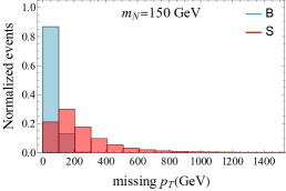
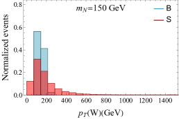
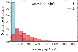
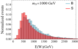
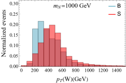
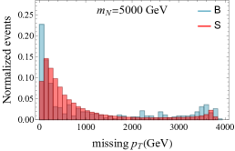
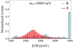
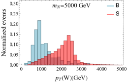
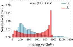
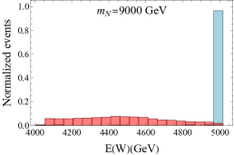
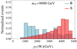
Figure 8: The normalized signal and background distributions $e$-flavored HNL at 10 TeV. The left column refers to the missing $p_{T}$ distribution after pre-selection and central $W$ cut. The middle column refers to $E(W)$ distribution after missing $p_{T}$ cuts. The right column refers to $p_{T}(W)$ distribution after $E(W)$ cut. Blue and red bins represent background and signal distributions, respectively.

5.5 Projected Sensitivities

After fully implementing the analysis, we evaluate and present the projected sensitivities at muon colliders here. We show the 95% exclusion limits of $|U_{\mu}|^{2}$ and $|U_{e}|^{2}$ at muon collider with $\sqrt{s}=3$ TeV and 10 TeV in Figure 9. The $\mu$-flavored HNL can be well-probed due to $t$-channel signal enhancement. The value of $|U_{\mu}|^{2}$ can be probed down to $O(10^{-7})\sim O(10^{-4})$ at 10 TeV and to $O(10^{-6})\sim O(10^{-4})$ at 3 TeV. For the $e$-flavored case represented by the blue line, the exclusion limit of $|U_{e}|^{2}$ is between $O(10^{-3})\%$ to $O(10^{-2})\%$. The $\tau$-flavored HNL has similar signal-background considerations as the electron case. We rescale both the signal and background by 40%, which accounts for a $\sim$60% efficiency for the three-prong $\tau$ decays, as a rough estimation of $\tau$-flavor sensitivities in green curves.

Note that for the $\mu$-flavored case, the sensitivities worsen at the low-$m_{N}$ region. First, this reduction in sensitivity is partially from the lower efficiency in signal detection due to the boosted forward decays discussed earlier (as shown in Table 9 and 10). The other reason is that the missing $p_{T}$ distribution tends to shift from high missing $p_{T}$ to low missing $p_{T}$ as $m_{N}$ increases, which gradually overlaps with the background (as shown in Figure 5 and 5). On the other hand, as $m_{N}$ increases, the $p_{T}(W)$ distribution starts to differ in the background and signal, which improves the sensitivity in high-mass benchmarks.

We also show the projected sensitivities together with LHC and proposed future colliders in Figure 10 for the $\mu$-flavored HNL, which is a benchmark commonly used in future collider studies Bose:2022obr ; Narain:2022qud ; Black:2022cth . At HL-LHC, we can probe $|U_{\mu}|^{2}$ to around $10^{-3}$. The future proton-proton collider could improve $|U_{\mu}|^{2}$ by one or two orders of magnitudes. The coverage in HNL mass $m_{N}$ at LHeC, FCC-he, and ILC are limited by the kinematics from the collision energy. We can see high energy muon colliders uniquely probe large new parameter space on the $|U_{\mu}|^{2}-m_{N}$ plane.

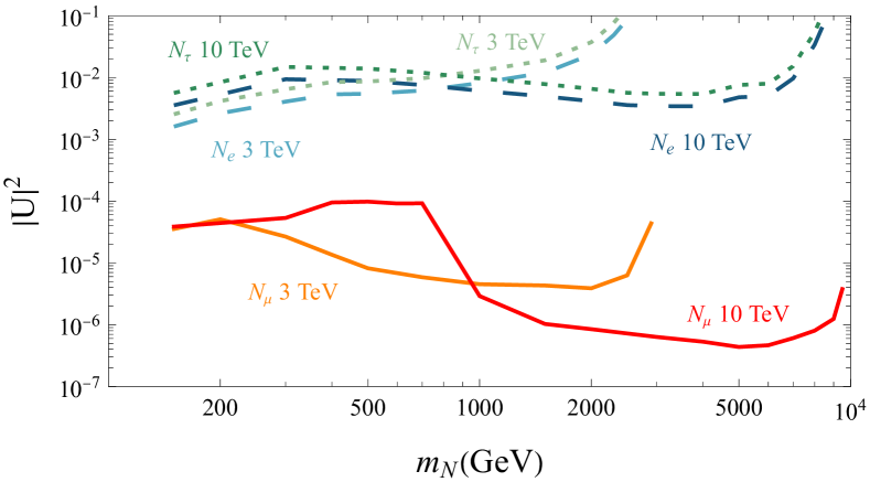
Figure 9: The 95% projected sensitivity of $|U_{\mu}|^{2}$, $|U_{e}|^{2}$ and $|U_{\tau}|^{2}$ as a function of HNL mass $m_{N}$ at 3 and 10 TeV muon collider.

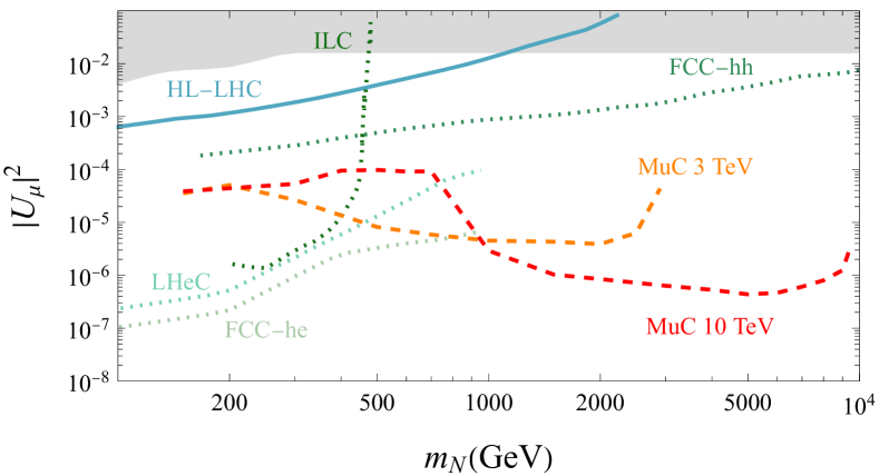
Figure 10: The 95% exclusion limits on the $|U_{\mu}|^{2}$-$m_{N}$ plane at different experimental facilities including LHC Izaguirre:2015pga ; Drewes:2019fou ; Pascoli:2018heg and proposed future colliders (LHeC and FCC-he Antusch:2019eiz , FCC-hh Pascoli:2018heg ; Antusch:2016ejd ,ILC Mekala:2022cmm ; Antusch:2016vyf ).

Note that besides the direct production and search for HNLs, one can also gain knowledge on the HNLs through other precision measurements. For instance, the HNLs mixing with the SM neutrinos changes the $Z$ boson invisible decay width, which dominates the existing constraints on the mixing angle at high HNL mass. For future electroweak factories, such as the FCC-ee FCC:2018evy and CEPC CEPCStudyGroup:2018ghi ; An:2018dwb ; CEPCPhysicsStudyGroup:2022uwl program, one can also derive complementary constraints, which will be limited by the theoretical uncertainties and systematic uncertainties associated with the precision observables. We anticipate the sensitivity to reach around $10^{-4}$ level from a back-in-the-envelope estimation, and certainly, a full study is in high demand.

6 Conclusion

In this paper, we study the unique physics potential of muon colliders in probing heavy neutral leptons. Two benchmark setup for muon colliders are used: $\sqrt{s}=3$ TeV with integrated luminosity $1\leavevmode\nobreak\ \text{ab}^{-1}$ and $\sqrt{s}=10$ TeV with integrated luminosity $10\leavevmode\nobreak\ \text{ab}^{-1}$. For simplicity, we parametrize the HNL in terms of its mass $m_{N}$ plus the squared mixing angle $|U_{\ell}|^{2}$ with the “active” SM neutrino. We focus on the regime $m_{h}<m_{N}<\sqrt{s}$ where the heavy neutrino promptly decays into massive gauge bosons and Higgs bosons. For the interesting lower $m_{N}$ values, we leave it to the future study due to a different consideration for the leading signal production and background composition.

Muon collider is uniquely advantageous for the muon-flavored HNL $N_{\mu}$ due to the dominance of $t$-channel processes that avoids the $1/s$ suppression. While for $e$- and $\tau$-flavored HNL, the leading 2-to-2 production processes are the $s$-channel diagrams. One also needs to consider the vector boson fusion processes for high-energy muon colliders. To carefully handle the VBF processes, we incorporate the structure functions of the muons, including the EW processes, and compare them with the fixed order calculations in various sub-processes. We adopt different treatments of the VBF processes on a process-by-process basis with corresponding physics considerations. We select the $N_{\ell}$ decay channel of $N_{\ell}\rightarrow\ell^{-}W^{+}$ followed by hadronic $W$ boson decay. Avoiding the detailed jet analysis, we include the background from both hadronic $W$ and hadronic $Z$ processes and adopt coarse binning and cuts on the hadronic gauge bosons. Therefore our final states are $\ell^{-}W^{+}$ plus other particles beyond our detector cut for the signal part and $\ell^{-}W^{+}(Z)$ plus “invisible” parts.

We adopt a cut-based analysis for HNL signal-background separation on the generated events. After imposing the mass window for the invariant mass of the HNL decay product system, we focus on the distribution of missing transverse momentum, the energy, and the transverse momentum of the hadronically decaying $W$ boson. We show the 95% exclusion limit in the $|U_{\ell}|^{2}-m_{N}$ plane. For the muon-flavored case, future high energy muon colliders can probe $|U_{\mu}|^{2}$ down to like $O(10^{-7})-O(10^{-5})$ due to the $t$-channel enhancement. For the electron case, the constraint on $|U_{e}|^{2}$ can be probed in a wide mass range for around $10^{-3}$. The results of the tau-flavored case are similar to the results of the electron case.

While the results in this work already show the promising physics potential for HNLs at future high-energy muon colliders, we have yet to use all the decay channels for the HNLs. For instance, one can study the leptonic decays of the HNLs, new production channels, and also with angular distribution to identify more properties of the HNLs. One can also study the long-lived signatures for HNLs below the tens of the GeV regime. These future directions can further reveal the physics in the neutrino sector and complete our picture of the muon collider potential.

Appendix A Cutflow table

In this appendix, we show the detailed cut flow tables for several of our benchmark signals and backgrounds. The cross sections after pre-selections are reported in section 4, and the optimization analysis follows the descriptions in section 5.

Background process	Central $W$	Mass window 150/1000/5000/9000 GeV	Optimization
$\mu^{+}\mu^{-}\longrightarrow W^{+}e^{-}\bar{\nu}_{e}$	96.82%	0.010/0.11/1.7/27.51%	0.010/0.080/0.43/0.61%
$\mu^{+}\mu^{-}\longrightarrow\mu^{+}\mu^{-}W^{+}e^{-}\bar{\nu}_{e}$	41.63%	1.4/0.77/0.017/0.00081%	0.021/0.28/0.011/0.00023%
$\mu^{+}\mu^{-}\longrightarrow\mu^{-}\bar{\nu}_{\mu}W^{+}e^{-}e^{+}$	17.69%	0.39/0.45/0.013/0.00028%	0.045/0.15/0.0067/0.00014%
$\mu^{+}\mu^{-}\longrightarrow N_{e}\bar{\nu}_{e}$	Central $W$	Mass window	Optimization
$m_{N}=150$ GeV	99.62%	99.62%	99.16%
$m_{N}=1000$ GeV	98.05%	98.05%	97.99%
$m_{N}=5000$ GeV	98.94%	98.94%	98.53%
$m_{N}=9000$ GeV	99.35%	99.35%	95.58%
$\mu^{+}\mu^{-}\longrightarrow\bar{\nu}_{\mu}\nu_{\mu}N_{e}\bar{\nu}_{e}$	Central $W$	Mass window	Optimization
$m_{N}=150$ GeV	83.34%	83.34%	64.97%
$m_{N}=1000$ GeV	93.48%	93.48%	79.67%
$m_{N}=5000$ GeV	99.02%	99.02%	88.15%
$m_{N}=9000$ GeV	99.78%	99.78%	68.87%
$\mu^{+}\mu^{-}\longrightarrow\mu^{+}\mu^{-}N_{e}\bar{\nu}_{e}$	Central $W$	Mass window	Optimization
$m_{N}=150$ GeV	77.69%	77.69%	61.32%
$m_{N}=1000$ GeV	93.06%	93.06%	80.30%
$m_{N}=5000$ GeV	99.08%	99.08%	85.68%
$m_{N}=9000$ GeV	100%	100%	59.81%

Table 13: Cutflow table for $N_{e}$ at 10 TeV. All processes after pre-selection is set to 100%.

Background process	Central $W$	Mass window 150/500/1500/2500 GeV	Optimization
$\mu^{+}\mu^{-}\longrightarrow W^{+}\mu^{-}\bar{\nu}_{\mu}$	90.37%	0.56/3.6/3.9/2.4%	0.56/1.1/1.7/1.2%
$\mu^{+}\mu^{-}\longrightarrow Z\mu^{+}\mu^{-}$	10.40%	0/0.79/0.22/0.090%	0/0.084/0/0%
$\mu^{+}\mu^{-}\longrightarrow\mu^{+}\mu^{-}W^{+}\mu^{-}\bar{\nu}_{\mu}$	62.15%	2.7/2.6/0.31/0.021%	0/2.4/0.30/0.021%
$\mu^{+}\mu^{-}\longrightarrow\bar{\nu}_{\mu}\nu_{\mu}W^{+}\mu^{-}\bar{\nu}_{\mu}$	86.21%	3.9/3.0/0.35/0.42%	1.2/1.3/0.070/0.35%
$\mu^{+}\mu^{-}\longrightarrow N_{\mu}\bar{\nu}_{\mu}$	Central $W$	Mass window	Optimization
$m_{N}=150$ GeV	22.09%	22.09%	21.80%
$m_{N}=500$ GeV	91.20%	91.20%	77.59%
$m_{N}=1500$ GeV	99.87%	99.87%	89.79%
$m_{N}=2500$ GeV	99.96%	99.96%	92.09%

Table 14: Cutflow table for $N_{\mu}$ at 3 TeV. All processes after pre-selection is set to 100%.

Background process	Central $W$	Mass window 150/1000/5000/9000 GeV	Optimization
$\mu^{+}\mu^{-}\longrightarrow W^{+}\mu^{-}\bar{\nu}_{\mu}$	89.14%	0.28/2.4/3.2/1.6%	0.28/0.42/1.1/0.80%
$\mu^{+}\mu^{-}\longrightarrow Z\mu^{+}\mu^{-}$	1.60%	0/0.085/0.039/0.016%	0/0.051/0/0%
$\mu^{+}\mu^{-}\longrightarrow\mu^{+}\mu^{-}W^{+}\mu^{-}\bar{\nu}_{\mu}$	43.39%	1.6/0.75/0.011/0%	0/0.73/0.0083/0%
$\mu^{+}\mu^{-}\longrightarrow N_{\mu}\bar{\nu}_{\mu}$	Central $W$	Mass window	Optimization
$m_{N}=150$ GeV	55.04%	55.04%	55.04%
$m_{N}=1000$ GeV	54.75%	54.75%	51.63%
$m_{N}=5000$ GeV	99.93%	99.93%	97.46%
$m_{N}=9000$ GeV	99.99%	99.99%	98.27%

Table 15: Cutflow table for $N_{\mu}$ at 10 TeV. All processes after pre-selection is set to 100%.

Background process	Central $W$	Mass window 150/500/1500/2500 GeV	Optimization
$\mu^{+}\mu^{-}\longrightarrow W^{+}e^{-}\bar{\nu}_{e}$	92.97%	0.014/0.14/1.5/18%	0.014/0.056/0.28/0.43%
$\mu^{+}\mu^{-}\longrightarrow\mu^{+}\mu^{-}W^{+}e^{-}\bar{\nu}_{e}$	64.22%	2.9/2.4/0.23/0.0011%	0.0088/0.013/0.0017/0%
$\mu^{+}\mu^{-}\longrightarrow\mu^{-}\bar{\nu}_{\mu}W^{+}e^{-}e^{+}$	33.46%	0.91/1.7/0.21/0.031%	0/0.0069/0.0030/0%
$\mu^{+}\mu^{-}\longrightarrow\bar{\nu}_{\mu}\nu_{\mu}W^{+}e^{-}\bar{\nu}_{e}$	84.05%	0.034/4.4/2.2/1.1%	0/0/0/0%
$\mu^{+}\mu^{-}\longrightarrow N_{e}\bar{\nu}_{e}$	Central $W$	Mass window	Optimization
$m_{N}=150$ GeV	98.80%	98.80%	97.08%
$m_{N}=500$ GeV	97.68%	97.68%	93.16%
$m_{N}=1500$ GeV	98.90%	98.90%	67.37%
$m_{N}=2500$ GeV	98.97%	98.97%	42.43%
$\mu^{+}\mu^{-}\longrightarrow\bar{\nu}_{\mu}\nu_{\mu}N_{e}\bar{\nu}_{e}$	Central $W$	Mass window	Optimization
$m_{N}=150$ GeV	87.85%	87.85%	28.3%
$m_{N}=500$ GeV	96.64%	96.64%	9.52%
$m_{N}=1500$ GeV	98.98%	98.98%	12.3%
$m_{N}=2500$ GeV	99.47%	99.47%	3.09%

Table 16: Cutflow table for $N_{e}$ at 3 TeV. All processes after pre-selection is set to 100%.

Appendix B Helicity Amplitudes

We show the helicity amplitudes of the 2-to-2 signal production chanel $\mu^{-}\mu^{+}\rightarrow N_{\mu}\bar{\nu}_{\mu}$ in the center-of-mass frame. For simplicity, the muon and neutrino masses are set to zero. The subscripts refer to the helicities of the particles $(\mu^{-},\leavevmode\nobreak\ \mu^{+},\leavevmode\nobreak\ N,\leavevmode\nobreak\ \bar{\nu})$ respectively. We choose the convention that the incoming $\mu^{-}$ is along the positive $z$ axis direction and the outcoming $N_{\mu}$ is emitted along the direction with polar angle $\theta$ and azimuthal angle $\phi=0$. The angular dependent part is expressed in terms of the Wigner D functions $d_{m,m^{\prime}}^{l}$.

For $s$-channel diagram, the non-zero helicity amplitudes $\mathcal{M}_{(\mu^{-},\leavevmode\nobreak\ \mu^{+},\leavevmode\nobreak\ N,\leavevmode\nobreak\ \bar{\nu})}$ are given by:

$$\mathcal{M}^{(s)}_{-+-+}=\frac{-ig^{2}U_{\mu}\cos(2\theta_{W})}{2\cos^{2}\theta_{W}}\,\frac{s}{s-M_{Z}^{2}}\sqrt{1-\frac{m_{N}^{2}}{s}}\ d_{1,1}^{1}$$ (23)

$$\mathcal{M}^{(s)}_{+--+}=\frac{-ig^{2}U_{\mu}\sin^{2}\theta_{W}}{\cos^{2}\theta_{W}}\,\frac{s}{s-M_{Z}^{2}}\sqrt{1-\frac{m_{N}^{2}}{s}}\ d_{1,-1}^{1}$$ (24)

$$\mathcal{M}^{(s)}_{+-++}=\frac{ig^{2}U_{\mu}\sin^{2}\theta_{W}}{\sqrt{2}\cos^{2}\theta_{W}}\,\frac{m_{N}\sqrt{s}}{s-M_{Z}^{2}}\sqrt{1-\frac{m_{N}^{2}}{s}}\ d_{1,0}^{1}$$ (25)

$$\mathcal{M}^{(s)}_{-+++}=\frac{-ig^{2}U_{\mu}\cos(2\theta_{W})}{2\sqrt{2}\cos^{2}\theta_{W}}\,\frac{m_{N}\sqrt{s}}{s-M_{Z}^{2}}\sqrt{1-\frac{m_{N}^{2}}{s}}\ d_{1,0}^{1}$$ (26)

where $\theta_{W}$ is the Weinberg angle.

For $t$-channel diagram, the non-zero helicity amplitudes are written as:

$$\mathcal{M}^{(t)}_{-+-+}=\frac{2ig^{2}U_{\mu}\cdot s\sqrt{1-\frac{m_{N}^{2}}{s}}\cdot d_{1,1}^{1}}{(s-m_{N}^{2})(\cos\theta-1)-2M_{W}^{2}}$$ (27)

$$\mathcal{M}^{(t)}_{-+++}=\frac{-\sqrt{2}ig^{2}U_{\mu}\cdot m_{N}\sqrt{s}\sqrt{1-\frac{m_{N}^{2}}{s}}\cdot d_{1,0}^{1}}{(s-m_{N}^{2})(\cos\theta-1)-2M_{W}^{2}}$$ (28)

In the massless $N_{\mu}$ case, the amplitude for the final helicity $\pm\pm$ states are vanished.

References

- (1) M. Boscolo, J.-P. Delahaye and M. Palmer, The future prospects of muon colliders and neutrino factories, Rev. Accel. Sci. Tech. 10 (2019) 189 [1808.01858].
- (2) J.P. Delahaye, M. Diemoz, K. Long, B. Mansoulié, N. Pastrone, L. Rivkin et al., Muon Colliders, 1901.06150.
- (3) H. Al Ali et al., The muon Smasher’s guide, Rept. Prog. Phys. 85 (2022) 084201 [2103.14043].
- (4) K.M. Black et al., Muon Collider Forum Report, 2209.01318.
- (5) M. Narain et al., The Future of US Particle Physics – The Snowmass 2021 Energy Frontier Report, 2211.11084.
- (6) T. Bose et al., Report of the Topical Group on Physics Beyond the Standard Model at Energy Frontier for Snowmass 2021, 2209.13128.
- (7) C. Aime et al., Muon Collider Physics Summary, 2203.07256.
- (8) International Muon Collider collaboration, The Muon Collider, JACoW IPAC2022 (2022) 821.
- (9) F. Zimmermann, Accelerator Technology and Beam Physics of Future Colliders, Front. in Phys. 10 (2022) 888395.
- (10) S.M. Bilenky and B. Pontecorvo, Lepton Mixing and Neutrino Oscillations, Phys. Rept. 41 (1978) 225.
- (11) Super-Kamiokande collaboration, Measurement of the flux and zenith angle distribution of upward through going muons by Super-Kamiokande, Phys. Rev. Lett. 82 (1999) 2644 [hep-ex/9812014].
- (12) Super-Kamiokande collaboration, Evidence for oscillation of atmospheric neutrinos, Phys. Rev. Lett. 81 (1998) 1562 [hep-ex/9807003].
- (13) SNO collaboration, Direct evidence for neutrino flavor transformation from neutral current interactions in the Sudbury Neutrino Observatory, Phys. Rev. Lett. 89 (2002) 011301 [nucl-ex/0204008].
- (14) KamLAND collaboration, First results from KamLAND: Evidence for reactor anti-neutrino disappearance, Phys. Rev. Lett. 90 (2003) 021802 [hep-ex/0212021].
- (15) S.M. Bilenky, Neutrino masses, mixing and oscillations, Prog. Part. Nucl. Phys. 57 (2006) 61 [hep-ph/0510175].
- (16) S.M. Bilenky, Majorana neutrino mixing, J. Phys. G 32 (2006) R127 [hep-ph/0511227].
- (17) M.C. Gonzalez-Garcia and M. Maltoni, Phenomenology with Massive Neutrinos, Phys. Rept. 460 (2008) 1 [0704.1800].
- (18) S.F. King and C. Luhn, Neutrino Mass and Mixing with Discrete Symmetry, Rept. Prog. Phys. 76 (2013) 056201 [1301.1340].
- (19) S.M. Bilenky, Neutrino in Standard Model and beyond, Phys. Part. Nucl. 46 (2015) 475 [1501.00232].
- (20) Particle Data Group collaboration, Review of Particle Physics, PTEP 2022 (2022) 083C01.
- (21) J.D. Bjorken and C.H. Llewellyn Smith, Spontaneously Broken Gauge Theories of Weak Interactions and Heavy Leptons, Phys. Rev. D 7 (1973) 887.
- (22) P. Minkowski, at a Rate of One Out of Muon Decays?, Phys. Lett. B 67 (1977) 421.
- (23) O. Sawada and A. Sugamoto, eds., Proceedings: Workshop on the Unified Theories and the Baryon Number in the Universe: Tsukuba, Japan, February 13-14, 1979, (Tsukuba, Japan), Natl.Lab.High Energy Phys., 1979.
- (24) M. Gell-Mann, P. Ramond and R. Slansky, Complex Spinors and Unified Theories, Conf. Proc. C 790927 (1979) 315 [1306.4669].
- (25) R.N. Mohapatra and G. Senjanovic, Neutrino Mass and Spontaneous Parity Nonconservation, Phys. Rev. Lett. 44 (1980) 912.
- (26) T. Yanagida, Horizontal Symmetry and Masses of Neutrinos, Prog. Theor. Phys. 64 (1980) 1103.
- (27) J. Schechter and J.W.F. Valle, Neutrino Masses in SU(2) x U(1) Theories, Phys. Rev. D 22 (1980) 2227.
- (28) D. Chang and R.N. Mohapatra, Comment on the ’Seesaw’ Mechanism for Small Neutrino Masses, Phys. Rev. D 32 (1985) 1248.
- (29) P. Langacker and D. London, Mixing Between Ordinary and Exotic Fermions, Phys. Rev. D 38 (1988) 886.
- (30) M. Dittmar, A. Santamaria, M.C. Gonzalez-Garcia and J.W.F. Valle, Production Mechanisms and Signatures of Isosinglet Neutral Heavy Leptons in Decays, Nucl. Phys. B 332 (1990) 1.
- (31) A.Y. Smirnov, Seesaw enhancement of lepton mixing, Phys. Rev. D 48 (1993) 3264 [hep-ph/9304205].
- (32) A. Strumia and F. Vissani, Neutrino masses and mixings and…, hep-ph/0606054.
- (33) R.N. Mohapatra and A.Y. Smirnov, Neutrino Mass and New Physics, Ann. Rev. Nucl. Part. Sci. 56 (2006) 569 [hep-ph/0603118].
- (34) J. Kersten and A.Y. Smirnov, Right-Handed Neutrinos at CERN LHC and the Mechanism of Neutrino Mass Generation, Phys. Rev. D 76 (2007) 073005 [0705.3221].
- (35) S. Davidson, E. Nardi and Y. Nir, Leptogenesis, Phys. Rept. 466 (2008) 105 [0802.2962].
- (36) A. Kusenko, Sterile neutrinos: The Dark side of the light fermions, Phys. Rept. 481 (2009) 1 [0906.2968].
- (37) B. Dasgupta and A.Y. Smirnov, Leptonic CP Violation Phases, Quark-Lepton Similarity and Seesaw Mechanism, Nucl. Phys. B 884 (2014) 357 [1404.0272].
- (38) N. Arkani-Hamed and Y. Grossman, Light active and sterile neutrinos from compositeness, Phys. Lett. B 459 (1999) 179 [hep-ph/9806223].
- (39) Y. Grossman and D.J. Robinson, Composite Dirac Neutrinos, JHEP 01 (2011) 132 [1009.2781].
- (40) Z. Chacko, P.J. Fox, R. Harnik and Z. Liu, Neutrino Masses from Low Scale Partial Compositeness, JHEP 03 (2021) 112 [2012.01443].
- (41) P. Cox, T. Gherghetta and M.D. Nguyen, Light sterile neutrinos and a high-quality axion from a holographic Peccei-Quinn mechanism, Phys. Rev. D 105 (2022) 055011 [2107.14018].
- (42) M.S. Chanowitz, M.A. Furman and I. Hinchliffe, Weak Interactions of Ultraheavy Fermions. 2., Nucl. Phys. B 153 (1979) 402.
- (43) A. Pilaftsis, CP violation and baryogenesis due to heavy Majorana neutrinos, Phys. Rev. D 56 (1997) 5431 [hep-ph/9707235].
- (44) E. Ma and U. Sarkar, Neutrino masses and leptogenesis with heavy Higgs triplets, Phys. Rev. Lett. 80 (1998) 5716 [hep-ph/9802445].
- (45) T. Asaka and M. Shaposhnikov, The MSM, dark matter and baryon asymmetry of the universe, Phys. Lett. B 620 (2005) 17 [hep-ph/0505013].
- (46) A.M. Abdullahi et al., The Present and Future Status of Heavy Neutral Leptons, in 2022 Snowmass Summer Study, 3, 2022 [2203.08039].
- (47) H.B. Thacker and J.J. Sakurai, Lifetimes and branching ratios of heavy leptons, Phys. Lett. B 36 (1971) 103.
- (48) J.C. Helo, S. Kovalenko and I. Schmidt, Sterile neutrinos in lepton number and lepton flavor violating decays, Nucl. Phys. B 853 (2011) 80 [1005.1607].
- (49) J.C. Helo, M. Hirsch and S. Kovalenko, Heavy neutrino searches at the LHC with displaced vertices, Phys. Rev. D 89 (2014) 073005 [1312.2900].
- (50) J. Liu, Z. Liu, L.-T. Wang and X.-P. Wang, Seeking for sterile neutrinos with displaced leptons at the LHC, JHEP 07 (2019) 159 [1904.01020].
- (51) A. Maiezza, M. Nemevšek and F. Nesti, Lepton Number Violation in Higgs Decay at LHC, Phys. Rev. Lett. 115 (2015) 081802 [1503.06834].
- (52) B. Batell, M. Pospelov and B. Shuve, Shedding Light on Neutrino Masses with Dark Forces, JHEP 08 (2016) 052 [1604.06099].
- (53) S. Antusch, E. Cazzato and O. Fischer, Displaced vertex searches for sterile neutrinos at future lepton colliders, JHEP 12 (2016) 007 [1604.02420].
- (54) S. Antusch, E. Cazzato and O. Fischer, Sterile neutrino searches via displaced vertices at LHCb, Phys. Lett. B 774 (2017) 114 [1706.05990].
- (55) G. Cottin, J.C. Helo and M. Hirsch, Searches for light sterile neutrinos with multitrack displaced vertices, Phys. Rev. D 97 (2018) 055025 [1801.02734].
- (56) A. Abada, N. Bernal, M. Losada and X. Marcano, Inclusive Displaced Vertex Searches for Heavy Neutral Leptons at the LHC, JHEP 01 (2019) 093 [1807.10024].
- (57) M. Drewes and J. Hajer, Heavy Neutrinos in displaced vertex searches at the LHC and HL-LHC, JHEP 02 (2020) 070 [1903.06100].
- (58) K. Bondarenko, A. Boyarsky, M. Ovchynnikov, O. Ruchayskiy and L. Shchutska, Probing new physics with displaced vertices: muon tracker at CMS, Phys. Rev. D 100 (2019) 075015 [1903.11918].
- (59) NA3 collaboration, Direct Photon Production From Pions and Protons at 200-GeV/, Z. Phys. C 31 (1986) 341.
- (60) WA66 collaboration, Search for Heavy Neutrino Decays in the BEBC Beam Dump Experiment, Phys. Lett. B 160 (1985) 207.
- (61) M. Gronau, C.N. Leung and J.L. Rosner, Extending Limits on Neutral Heavy Leptons, Phys. Rev. D 29 (1984) 2539.
- (62) S.A. Baranov et al., Search for heavy neutrinos at the IHEP-JINR neutrino detector, Phys. Lett. B 302 (1993) 336.
- (63) NOMAD collaboration, Search for heavy neutrinos mixing with tau neutrinos, Phys. Lett. B 506 (2001) 27 [hep-ex/0101041].
- (64) FMMF collaboration, Search for neutral weakly interacting massive particles in the Fermilab Tevatron wide band neutrino beam, Phys. Rev. D 52 (1995) 6.
- (65) SHiP collaboration, A facility to Search for Hidden Particles (SHiP) at the CERN SPS, 1504.04956.
- (66) P. Ballett, T. Boschi and S. Pascoli, Heavy Neutral Leptons from low-scale seesaws at the DUNE Near Detector, JHEP 03 (2020) 111 [1905.00284].
- (67) FASER collaboration, FASER’s physics reach for long-lived particles, Phys. Rev. D 99 (2019) 095011 [1811.12522].
- (68) FASER collaboration, FASER: Forward Search Experiment at the LHC, PoS EPS-HEP2021 (2022) 705.
- (69) CHARM collaboration, A Search for Decays of Heavy Neutrinos in the Mass Range 0.5-GeV to 2.8-GeV, Phys. Lett. B 166 (1986) 473.
- (70) CHARM II collaboration, Search for heavy isosinglet neutrinos, Phys. Lett. B 343 (1995) 453.
- (71) NuTeV, E815 collaboration, Search for neutral heavy leptons in a high-energy neutrino beam, Phys. Rev. Lett. 83 (1999) 4943 [hep-ex/9908011].
- (72) F. del Aguila, J.A. Aguilar-Saavedra and R. Pittau, Heavy neutrino signals at large hadron colliders, JHEP 10 (2007) 047 [hep-ph/0703261].
- (73) D. Alva, T. Han and R. Ruiz, Heavy Majorana neutrinos from fusion at hadron colliders, JHEP 02 (2015) 072 [1411.7305].
- (74) C. Degrande, O. Mattelaer, R. Ruiz and J. Turner, Fully-Automated Precision Predictions for Heavy Neutrino Production Mechanisms at Hadron Colliders, Phys. Rev. D 94 (2016) 053002 [1602.06957].
- (75) E. Accomando, L. Delle Rose, S. Moretti, E. Olaiya and C.H. Shepherd-Themistocleous, Extra Higgs boson and Z′ as portals to signatures of heavy neutrinos at the LHC, JHEP 02 (2018) 109 [1708.03650].
- (76) S. Pascoli, R. Ruiz and C. Weiland, Heavy neutrinos with dynamic jet vetoes: multilepton searches at , 27, and 100 TeV, JHEP 06 (2019) 049 [1812.08750].
- (77) E. Fernández-Martínez, X. Marcano and D. Naredo-Tuero, HNL mass degeneracy: implications for low-scale seesaws, LNV at colliders and leptogenesis, 2209.04461.
- (78) A. Abada, P. Escribano, X. Marcano and G. Piazza, Collider searches for heavy neutral leptons: beyond simplified scenarios, Eur. Phys. J. C 82 (2022) 1030 [2208.13882].
- (79) E. Arganda, M.J. Herrero, X. Marcano and C. Weiland, Exotic jj events from heavy ISS neutrinos at the LHC, Phys. Lett. B 752 (2016) 46 [1508.05074].
- (80) A. Ismail, S. Jana and R.M. Abraham, Neutrino up-scattering via the dipole portal at forward LHC detectors, Phys. Rev. D 105 (2022) 055008 [2109.05032].
- (81) P.S.B. Dev, A. Pilaftsis and U.-k. Yang, New Production Mechanism for Heavy Neutrinos at the LHC, Phys. Rev. Lett. 112 (2014) 081801 [1308.2209].
- (82) A. Das and N. Okada, Bounds on heavy Majorana neutrinos in type-I seesaw and implications for collider searches, Phys. Lett. B 774 (2017) 32 [1702.04668].
- (83) A. Das, Pair production of heavy neutrinos in next-to-leading order QCD at the hadron colliders in the inverse seesaw framework, Int. J. Mod. Phys. A 36 (2021) 2150012 [1701.04946].
- (84) A. Das, P. Konar and A. Thalapillil, Jet substructure shedding light on heavy Majorana neutrinos at the LHC, JHEP 02 (2018) 083 [1709.09712].
- (85) A. Das, S. Jana, S. Mandal and S. Nandi, Probing right handed neutrinos at the LHeC and lepton colliders using fat jet signatures, Phys. Rev. D 99 (2019) 055030 [1811.04291].
- (86) A. Das and N. Okada, Inverse seesaw neutrino signatures at the LHC and ILC, Phys. Rev. D 88 (2013) 113001 [1207.3734].
- (87) S. Banerjee, P.S.B. Dev, A. Ibarra, T. Mandal and M. Mitra, Prospects of Heavy Neutrino Searches at Future Lepton Colliders, Phys. Rev. D 92 (2015) 075002 [1503.05491].
- (88) A. Blondel et al., Searches for long-lived particles at the future FCC-ee, Front. in Phys. 10 (2022) 967881 [2203.05502].
- (89) K. Mękała, J. Reuter and A.F. Żarnecki, Heavy neutrinos at future linear e+e− colliders, JHEP 06 (2022) 010 [2202.06703].
- (90) I. Chakraborty, H. Roy and T. Srivastava, Searches for heavy neutrinos at multi-TeV muon collider : a resonant leptogenesis perspective, 2206.07037.
- (91) A.G. Dias, C.A. de S. Pires, P.S. Rodrigues da Silva and A. Sampieri, A Simple Realization of the Inverse Seesaw Mechanism, Phys. Rev. D 86 (2012) 035007 [1206.2590].
- (92) S.S.C. Law and K.L. McDonald, Generalized inverse seesaw mechanisms, Phys. Rev. D 87 (2013) 113003 [1303.4887].
- (93) R.N. Mohapatra and J.W.F. Valle, Neutrino Mass and Baryon Number Nonconservation in Superstring Models, Phys. Rev. D 34 (1986) 1642.
- (94) E. Ma, Lepton Number Nonconservation in Superstring Models, Phys. Lett. B 191 (1987) 287.
- (95) E. Ma, Radiative inverse seesaw mechanism for nonzero neutrino mass, Phys. Rev. D 80 (2009) 013013 [0904.4450].
- (96) F. Bazzocchi, Minimal Dynamical Inverse See Saw, Phys. Rev. D 83 (2011) 093009 [1011.6299].
- (97) D. Wyler and L. Wolfenstein, Massless Neutrinos in Left-Right Symmetric Models, Nucl. Phys. B 218 (1983) 205.
- (98) E.K. Akhmedov, M. Lindner, E. Schnapka and J.W.F. Valle, Left-right symmetry breaking in NJL approach, Phys. Lett. B 368 (1996) 270 [hep-ph/9507275].
- (99) E.K. Akhmedov, M. Lindner, E. Schnapka and J.W.F. Valle, Dynamical left-right symmetry breaking, Phys. Rev. D 53 (1996) 2752 [hep-ph/9509255].
- (100) A. de Gouvêa, P.J. Fox, B.J. Kayser and K.J. Kelly, Three-body decays of heavy Dirac and Majorana fermions, Phys. Rev. D 104 (2021) 015038 [2104.05719].
- (101) A.B. Balantekin, A. de Gouvêa and B. Kayser, Addressing the Majorana vs. Dirac Question with Neutrino Decays, Phys. Lett. B 789 (2019) 488 [1808.10518].
- (102) A. Baha Balantekin and B. Kayser, On the Properties of Neutrinos, Ann. Rev. Nucl. Part. Sci. 68 (2018) 313 [1805.00922].
- (103) T. Han, Y. Ma and K. Xie, High energy leptonic collisions and electroweak parton distribution functions, Phys. Rev. D 103 (2021) L031301 [2007.14300].
- (104) G.L. Kane, W.W. Repko and W.B. Rolnick, The Effective W+-, Z0 Approximation for High-Energy Collisions, Phys. Lett. B 148 (1984) 367.
- (105) S. Dawson, The Effective W Approximation, Nucl. Phys. B 249 (1985) 42.
- (106) B. Fornal, A.V. Manohar and W.J. Waalewijn, Electroweak Gauge Boson Parton Distribution Functions, JHEP 05 (2018) 106 [1803.06347].
- (107) J. Chen, T. Han and B. Tweedie, Electroweak Splitting Functions and High Energy Showering, JHEP 11 (2017) 093 [1611.00788].
- (108) A. Costantini, F. De Lillo, F. Maltoni, L. Mantani, O. Mattelaer, R. Ruiz et al., Vector boson fusion at multi-TeV muon colliders, JHEP 09 (2020) 080 [2005.10289].
- (109) J. Alwall, R. Frederix, S. Frixione, V. Hirschi, F. Maltoni, O. Mattelaer et al., The automated computation of tree-level and next-to-leading order differential cross sections, and their matching to parton shower simulations, JHEP 07 (2014) 079 [1405.0301].
- (110) R. Ruiz, A. Costantini, F. Maltoni and O. Mattelaer, The Effective Vector Boson Approximation in high-energy muon collisions, JHEP 06 (2022) 114 [2111.02442].
- (111) C. Degrande, C. Duhr, B. Fuks, D. Grellscheid, O. Mattelaer and T. Reiter, UFO - The Universal FeynRules Output, Comput. Phys. Commun. 183 (2012) 1201 [1108.2040].
- (112) A. Atre, T. Han, S. Pascoli and B. Zhang, The Search for Heavy Majorana Neutrinos, JHEP 05 (2009) 030 [0901.3589].
- (113) A. Alloul, N.D. Christensen, C. Degrande, C. Duhr and B. Fuks, FeynRules 2.0 - A complete toolbox for tree-level phenomenology, Comput. Phys. Commun. 185 (2014) 2250 [1310.1921].
- (114) I.F. Ginzburg, Initial particle instability in muon collisions, Nucl. Phys. B Proc. Suppl. 51 (1996) 85 [hep-ph/9601272].
- (115) C. Dams and R. Kleiss, Singular cross-sections in muon colliders, Eur. Phys. J. C 29 (2003) 11 [hep-ph/0212301].
- (116) K. Melnikov and V.G. Serbo, Processes with the T channel singularity in the physical region: Finite beam sizes make cross-sections finite, Nucl. Phys. B 483 (1997) 67 [hep-ph/9601290].
- (117) E. Izaguirre and B. Shuve, Multilepton and Lepton Jet Probes of Sub-Weak-Scale Right-Handed Neutrinos, Phys. Rev. D 91 (2015) 093010 [1504.02470].
- (118) S. Antusch, O. Fischer and A. Hammad, Lepton-Trijet and Displaced Vertex Searches for Heavy Neutrinos at Future Electron-Proton Colliders, JHEP 03 (2020) 110 [1908.02852].
- (119) S. Antusch, E. Cazzato and O. Fischer, Sterile neutrino searches at future , , and colliders, Int. J. Mod. Phys. A 32 (2017) 1750078 [1612.02728].
- (120) FCC collaboration, FCC-ee: The Lepton Collider: Future Circular Collider Conceptual Design Report Volume 2, Eur. Phys. J. ST 228 (2019) 261.
- (121) CEPC Study Group collaboration, CEPC Conceptual Design Report: Volume 2 - Physics & Detector, 1811.10545.
- (122) F. An et al., Precision Higgs physics at the CEPC, Chin. Phys. C 43 (2019) 043002 [1810.09037].
- (123) CEPC Physics Study Group collaboration, The Physics potential of the CEPC. Prepared for the US Snowmass Community Planning Exercise (Snowmass 2021), in 2022 Snowmass Summer Study, 5, 2022 [2205.08553].
- (124) K. Mękała, J. Reuter and A.F. Żarnecki, Optimal search reach for heavy neutral leptons at a muon collider, 2301.02602.
- (125) T.H. Kwok, L. Li, T. Liu and A. Rock, Searching for Heavy Neutral Leptons at A Future Muon Collider, 2301.05177.