Continuous Trajectory Generation Based on Two-Stage GAN
Abstract
Simulating the human mobility and generating large-scale trajectories are of great use in many real-world applications, such as urban planning, epidemic spreading analysis, and geographic privacy protect. Although many previous works have studied the problem of trajectory generation, the continuity of the generated trajectories has been neglected, which makes these methods useless for practical urban simulation scenarios. To solve this problem, we propose a novel two-stage generative adversarial framework to generate the continuous trajectory on the road network, namely TS-TrajGen, which efficiently integrates prior domain knowledge of human mobility with model-free learning paradigm. Specifically, we build the generator under the human mobility hypothesis of the A* algorithm to learn the human mobility behavior. For the discriminator, we combine the sequential reward with the mobility yaw reward to enhance the effectiveness of the generator. Finally, we propose a novel two-stage generation process to overcome the weak point of the existing stochastic generation process. Extensive experiments on two real-world datasets and two case studies demonstrate that our framework yields significant improvements over the state-of-the-art methods.
Introduction
Modeling human mobility and generating synthetic yet realistic trajectories is crucial in many applications (Luca et al. 2021). On the one hand, synthetic trajectories are fundamental for urban planning, epidemic spreading analysis, and traffic control, e.g., simulating changes in urban mobility in the presence of new infrastructure or international events (Paola et al. 2019; Wang et al. 2021a). On the other hand, generating synthetic trajectories is a viable solution to protect the privacy of human mobility trajectory data (Pellungrini et al. 2017). The difficulty of open source sharing of trajectory data today is heavily due to privacy concerns, which hinders most existing data-driven studies. Using synthetic trajectories instead of real trajectories can not only preserve the utility of trajectory data, but also avoid leakage of user privacy. Therefore, in such cases, it is important to generate synthetic trajectories with good data utility.
In the last decades, the problem of trajectory generation has been widely studied. In the early stage, the researchers aim to build model-based methods to model the regularity of human mobility (Song et al. 2010; Jiang et al. 2016), such as temporal periodicity, spatial continuity. These methods assume that human mobility can be described by specific mobility patterns and thus can be modeled with finite parameters with explicit physical meanings. However, in fact, human mobility behaviors exhibit complex sequential transition regularities, which can be time-dependent and high-ordered. Thus, although these model-based methods have the advantage of being interpretable by design, their performance is limited due to the simplicity of the implemented mechanisms (Luca et al. 2021). To address the above limitation, the researchers propose model-free methods (Yin, Yang, and Ma 2018; Ouyang et al. 2018), mainly using neural network generative paradigms such as generative adversarial network and variational autoencoder. Unlike model-based methods, model-free methods abandon the extraction of specific human mobility patterns, and instead directly build a neural network to learn the distribution of the real data and generate trajectories from the same distribution.
However, comparing the above approaches, there are several key challenges remaining to be solved: (1) First, the problem of the continuity of the generated trajectories is ignored. The trajectories generated by current methods are not continuous routes on the road network, which makes these synthetic trajectories unusable for downstream applications like traffic simulation. (2) Second, those model-free methods without utilizing prior knowledge of human mobility fail to effectively generate continuous trajectories. (3) Third, the stochastic generation process of existing methods has the error accumulation problem, where the trajectory is randomly generated according to the probability given by the generator. However, once the generator predicts wrong, the process continues to generate under the wrong premise, which reduces the quality of the generated trajectory.
In this paper, we propose TS-TrajGen, a novel two-stage generative adversarial framework with spatial-temporal oriented designs in the generator, discriminator and generation process to tackle the above challenges. Specifically, we build the generator based on the human mobility hypothesis of the A* algorithm (Hart, Nilsson, and Raphael 1968) to address the first challenges. The A* algorithm is a heuristic search algorithm used extensively on the road network. In the A* hypothesis, human mobility behaviors are determined by two factors: the observed cost from the source road to the candidate road, and the expected cost from the candidate road to the destination. Combining above two costs, A* algorithm evaluates which candidate road is the best candidate to be searched, and then generates a heuristic best continuous trajectory. Therefore, our generator consists of two parts: an attention-based network to learn the observed cost, and a GAT-based network to estimate the expected cost. As for the second challenge, we combine the sequential reward with the mobility yaw reward to improve the effectiveness of the generator, which distinguish the trajectory from the perspective of time series similarity and spatial similarity respectively. For the third challenge, we propose a two-stage generation process to solve the problem of error accumulation. In the first stage, we construct the structural regions on the top of the road network and then generate the regional trajectory. In the second stage, we generate the continuous trajectory in the guidance of the regional trajectory.
To the best of our knowledge, we are the first to solve the continuous trajectory generation problem on the urban road network, through combining the A* algorithm with neural network. In addition, to improve the effectiveness and efficiency of the generation, we build a discriminator combining the sequential reward with mobility yaw reward and propose a two-stage generation process. Extensive experiments on two real-world trajectory data have demonstrated the effectiveness and robustness of our proposed framework.
Preliminary
A trajectory in the road network can be defined as a time-ordered sequence , where is a spatial-temporal point defined as a tuple . The is the road segment ID and the is the timestamp of . The continuous trajectory is a trajectory, where each segment pair is adjacent in the road network graph.
Definition 1.
Continuous Mobility Trajectory Generation. Given a real-world mobility trajectory dataset, generate a continuous mobility trajectory with a -parameterized generative model .
In general, the process of continuous mobility trajectory generation can be regarded as a Markov decision process (MDP). The state describes the current movement situation, composed of the current partial trajectory and the travel destination . The action is the next candidate road segment to move. The agent is the generative model, which model the human movement policy .
Definition 2.
Human Movement Policy. The human movement policy is the conditional probability of taking action in the state , which can be formulated as follows:
| (1) |
Thus, the generation process can be described as maximizing the probability of the generated trajectory as
| (2) |
The Proposed Framework
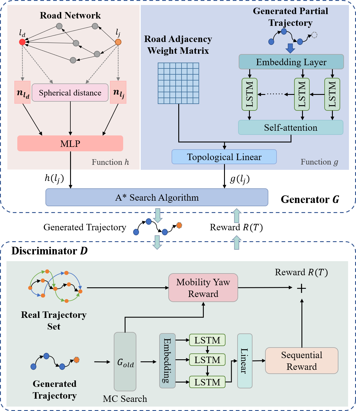
In this section, we first give a brief overview of our proposed framework and then describe each part of our framework in detail. We build a generator to learn the human movement policy , and a discriminator to generate the reward to guide the optimization process of the generator, which is represented in Figure 1. Besides, we propose a novel two-stage generation process to generate trajectories more accurately and efficiently. Finally, we introduce the training process of our proposed framework.
Modeling Human Movement Policy by Generator
As stated in Definition 2, the key factor that determines the human movement policy is the current state , which is described by current partial trajectory and the travel destination . To consider both the impact of the current partial trajectory and the impact of the travel destination, we adopt the hypothesis of A* algorithm to model the human movement policy . The A* algorithm is a heuristic search algorithm used extensively on the road network, which evaluates candidate road exactly based on the above two impacts as
| (3) |
where the function evaluates the observed cost of the current partial trajectory, and the function estimates the expected cost of arriving the destination through the candidate road .
Combining above two costs, A* algorithm learn the human movement policy as follows:
| (4) |
With the function , A* algorithm evaluates which candidate road is the best candidate to be searched, and then generates the heuristic best continuous trajectory.
However, there are two weak points for generating trajectories with the original A* algorithm. First, the original functions and are calculated based on the spherical distance between road segments, which makes it difficult to learn diverse human movement policy. Second, the spherical distance can not accurately estimate the expected cost. For example, although roads and are close in space, they may be one-way roads in two different directions on the road network, which makes the real expected cost between them greater than the spherical distance. Thus, we implement the functions and with the neural network to learn the human movement policy.
Function g().
To model the observed cost, we combine the LSTM network with the self-attention mechanism to learn the current moving state and then predict the observed cost with a topologically constrained linear layer.
First, given a current partial trajectory , we extract the spatial-temporal information through embedding each point into a dense vector as
| (5) |
where we encode the timestamp by mapping the weekday timestamp to a group of time slots (1 to 1440), and the weekend timestamp to another group time slots (1441 to 2880).
After embedding, we transform the current partial trajectory into a sequence of dense vectors . Then, we apply the LSTM network (Hochreiter and Schmidhuber 1997) to model the sequential trajectory moving state . We further leverage the dot-product attention mechanism (Vaswani et al. 2017) to enhance the latent moving state in the form of
| (6) |
where the function evaluates the correlation weight between the current moving state and the historical moving state through a dot-production method.
Finally, after capturing the enhanced moving state, we construct a topologically constrained linear layer to predict the observed conditional probability . In the topologically constrained linear layer, we introduce a topological adjacency weight into the linear layer, which is 1 when the candidate road is adjacent to the current road and 0 otherwise. With the topological adjacency weight, we set the conditional probability of the non-adjacent candidate road to zero, which ensures the continuity of the generated trajectory. The observed conditional probability is formulated as
| (7) |
where the parameter vector is the -th row of the weight matrix of the linear layer.
The observed cost can be calculated as the negative log of the conditional probability as
| (8) |
Function h().
To model the expected cost, we assume that a person usually needs to know the relative position of two roads in the road network and the distance between them when estimating the expect cost of getting from a candidate road to the destination. From this perspective, we use a graph attention network to extract the relative position information from the road network and calculate the spherical distance between two road segments. Based on above information, we finally use a multilayer perceptron network to estimate the expected cost .
First, we build a graph attention network (Veličković et al. 2018) to learn the structural road representation containing the relative position information. The update of the graph attention network can be given as
| (9) |
where is the matrix of road representation at the -th iteration, the -th row corresponds to the representation of road segment , and is the road adjacency matrix.
For initialization, we construct the road contextual embedding vectors and set . Given a road segment , we consider 6 kinds of road attributes, namely segment length, segment width, max speed limitation, lane number, road type, and longitude and latitude. We perform normalization on continuous attributes and one-hot encoding on discrete attributes, and concatenate the encoded attributes as the contextual embedding vector .
After obtaining the road representation, we use a multilayer perceptron network to predict the expected conditional probability from a candidate road to the destination as
| (10) |
where the and is the road representation of road and , and the is the spherical distance between them.
In the end, the expected cost is calculated as the negative log of the conditional probability as
| (11) |
Remark.
Compared with the original A* algorithm, our function is capable to model the diverse human movement policy with the introduction of temporal information and the sequential moving state. Besides, combining the structural road representation, the effectiveness of the expected cost is improved.
Enhancing Generator with Discriminator
In general, the generative adversarial network learned by a min-max game as follows
| (12) |
where denotes the sample from the real data distribution, denotes the sample generated by the generator, and is the -parameterized discriminator.
In the min-max game, the goal of the discriminator is to distinguish the input sample, and the generator optimizes itself based on the discriminator’s output signal, i.e., the reward as
| (13) |
In our framework, the input sample is a trajectory , which is a time-series with spatial information. Thus, we distinguish the input trajectory in terms of the time-series similarity and the spatial similarity, and generate corresponding reward as
| (14) |
where denotes the sequential reward from the time-series aspect, where we evaluate the similarity based on the hidden sequential transition pattern extracted by an LSTM network. denotes the mobility yaw reward from the spatial aspect, where we evaluate the similarity according to the trajectory’s mobility yaw distance from the real trajectories.
Sequential Reward.
To extract the sequential transition pattern, we build a sequential discriminator following the same steps in the function : we first embed the input trajectory, and then obtain the hidden sequential transition pattern based on an LSTM network. Then, we use a linear layer to predict the probability that the trajectory is real, which is the sequential reward as
| (15) |
where we further leverage the Monte Carlo search to evaluate the average sequential reward for the intermediate step in the trajectory.
This is because the trajectory from the generator is sequentially generated, which requires the discriminator to provide rewards for each step of the trajectory. However, current discriminator can not provide proper reward for the intermediate step. For the intermediate step , the current trajectory is still unfinished. This means that the reward, based on current sub-trajectory , only considers the sequential transition pattern of the current sub-trajectory but ignores the future outcome. Thus, following the previous work (Yu et al. 2017), we apply Monte Carlo search to evaluate the intermediate step. To do this, we first maintain an older version generator , which is the last step version of the current generator. Then, we use the to complete the current sub-trajectory by repeating Monte Carlo search times. The complete trajectories are then fed into the to generate sequential reward for the intermediate step.
Mobility Yaw Reward.
The mobility yaw distance of a input trajectory is defined as the minimum distance to the real trajectories set in the form of
| (16) |
where we leverage the widely-used trajectory distance metric DTW (Keogh 2002) to measure the mobility yaw distance, and the real trajectories set contains the real trajectories shared the same OD with the input trajectory .
Furthermore, we calculate the mobility yaw distance for each step of the trajectory by the Monte Carlo search. The mobility yaw reward is defined as the change in yaw distance as
| (17) |
where we further apply a normalization to dimensionless the change of mobility yaw distance.
The change in yaw distance indicates how much the current step’s mobility yaw distance has decreased compared to the previous step. The more the mobility yaw distance is decreased, the more correct the decision of the current step is. Correspondingly, the reward for the current step should be larger.
Two-Stage Generation Process
The stochastic generation process has the problem of error accumulation, where trajectory is randomly generated according to the probability given by the generator as
| (18) |
However, once the generator predicts wrong, the stochastic generation process continues to generate under the wrong premise state. Especially, when generating long trajectories, the probability of the generator making an error increases as the number of predictions made by the generator increases. This makes it difficult to reach the destination and reduces the quality of the generated trajectory.
To solve the above problem, we propose a novel two-stage generation process based on A* search. We first construct the structural regions above the road network. Then, we generate the regional trajectory in the first stage. In the second stage, we generate the continuous trajectory in the guidance of the regional trajectory. With the A* search, our generation process can roll back to correct the error, when the generator predicts incorrectly. Because, in the A* search, all possible trajectories currently searched are maintained, and the trajectory with the least cost (highest probability) is selected for searching each time. In addition, with the two-stage generation, not only the space and time complexity of the generation process is reduced, but the generation of long trajectories is also avoided.
Building Structural Region.
We leverage the multilevel graph partitioning algorithm KaFFPa (Sanders and Schulz 2013) to construct structural regions on the top of the road network. It partitions the graph into blocks under the constraint that the number of edges between blocks is minimized and the maximum block size does not exceed times the average block size. With the KaFFPa algorithm, we can obtain relatively independent structural regions of similar size, and the mapping relationship between road and region. Formally, we describe the mapping relationship between road and region as the mapping matrix , where each element is defined as
| (19) |
where the is the -th road segment in road segment set , and the is the -th structural region in region set .
Based on the mapping matrix , the region-level data can be obtained through mapping from the road-level data. Then, we use the same proposed adversarial generative framework to learn the region-level human movement policy. See the appendix for more details.
Regional Trajectory Generation.
In the first stage, we aim to generate the regional trajectory. At the beginning, we sample a tuple of origin and destination and the start timestamp from the historical OD matrix, which can be counted from the given real-world trajectory dataset. Then, we map the road-level origin and destination to the region-level origin and destination according to the road-to-region mapping relationship, where we map the to only if the . With the region-level origin and destination and the start timestamp as input, we generate regional trajectory based on the A* search and the region-level generator.
Road-level Continuous Trajectory Generation.
In the second stage, we generate the continuous trajectory in the guidance of the regional trajectory. In practice, we construct the boundary road segments set between each region and region , and count the visiting frequency of each boundary road segment in advance. Then, the regional trajectory can be mapped to the road-level, according to the Algorithm 1.
After obtaining the discontinuous road segment trajectory , we use the road-level generator to complete the trajectory between each pair in the , which is the final continuous trajectory. In this way, we only need to generate in a small structural region instead of the huge road network.
Training Process
At the beginning of the training, we use the trajectory next-location prediction task to pre-train the function and separately, as they model human movement policy from different perspectives. Then, we pre-train the sequential discriminator based on the generated trajectories and the real trajectories. After the pre-training, we follow the REINFORCE algorithm (Williams 1992) to generate the policy gradient by receiving the reward from the discriminator as
| (20) |
where is the parameter of the generator , is the generated trajectory, the reward is the sum of sequential reward and mobility yaw reward from the discriminator . Based on the policy gradient , parameter is updated by , where is the learning rate.
Experiment
We first evaluate TS-TrajGen in terms of macro-similarity and micro-similarity between the synthetic trajectories and the real trajectories. Next, we conduct two case studies: the trajectory next-location prediction and the traffic control simulation, to assess the utility of synthetic trajectories.
Experiment Setting
Dataset.
We use two real-world mobility dataset to measure the performance of our proposed framework. The BJ-Taxi dataset contains real GPS trajectory data of Beijing taxis for one week from November 1 to 7, 2015 within Beijing’s Fourth Ring Roads, which is sampled every minute. The Porto-Taxi dataset is originally released for a Kaggle trajectory prediction competition with a sample period of 15 seconds. For the two datasets, we collect corresponding road network information from the open street map, and then perform map maching (Yang and Gidofalvi 2018) to obtain real continuous trajectories. To eliminate abnormal trajectories, we remove trajectories with lengths less than 5 and trajectories with loops. The statistics of the two datasets after preprocessing are shown in Table 1. For each trajectory dataset, we randomly split the whole dataset into three parts in the ratio of 6:2:2: a training set, a validation set, and a test set.
| Data Statistics | BJ-Taxi | Porto-Taxi |
|---|---|---|
| Number of Taxis | 15,642 | 435 |
| Number of Roads | 40,306 | 11,095 |
| Number of Intersections | 16,927 | 5,184 |
| Number of Trajectories | 956,070 | 695,085 |
Comparative Benchmarks.
We compare TS-TrajGen with five baselines to validate the performance of our proposed framework: SeqGAN (Yu et al. 2017), SVAE (Huang et al. 2019), MoveSim (Feng et al. 2020), TSG (Wang et al. 2021b), and TrajGen (Cao and Li 2021). For more information about the baselines, please refer to the appendix.
Performance Criteria.
From the macro perspective, we mainly consider the overall distribution of the trajectory dataset. Following the common practice in previous works (Cao and Li 2021; Feng et al. 2020), we quantitatively assess the quality of the generated data by computing the similarity of 4 important mobility patterns between the generated and real data: the travel distance (Brockmann, Hufnagel, and Geisel 2006), the radius of gyration (González, Hidalgo, and Barabási 2008), the location distribution (Ouyang et al. 2018) and the OD flow (Simini et al. 2012). To obtain quantitative results, we use Jensen-Shannon Divergence to calculate the similarity on the four metrics. Refer to the appendix for more information on the metrics.
From the microscopic perspective, we focus on measuring the similarity between the real trajectories and the generated trajectories with the same OD. In practice, we use three widely used trajectory distance metrics to measure the micro similarity: Hausdorff distance (Xie, Li, and Phillips 2017), DTW (Keogh 2002), and EDR (Chen, Özsu, and Oria 2005). We randomly select 5,000 trajectories from the test set, and make the generative model generate the corresponding trajectory. Finally, the average distance between the generated trajectories and the real trajectories is taken as the evaluation result.
Evaluation Results
The evaluation results of macro-similarity and micro-similarity are shown in Table 2. In each row, the best result is highlighted in boldface and the second best is underlined. From the statistics, we can first conclude that our proposed TS-TrajGen significantly outperforms all baselines in terms of both macro-similarity metrics and micro-similarity metrics.
| Model\Metrics | BJ-Taxi | Porto-Taxi | ||||||||||||
|---|---|---|---|---|---|---|---|---|---|---|---|---|---|---|
| Macro-Similarity Metrics | Micro-Similarity Metrics | Macro-Similarity Metrics | Micro-Similarity Metrics | |||||||||||
| Distance | Radius | Location Frequency | OD Flow | Hausdorff | DTW | EDR | Distance | Radius | Location Frequency | OD Flow | Hausdorff | DTW | EDR | |
| SeqGAN | 0.4945 | 0.4717 | 0.1124 | 0.6519 | 13.85 | 199.51 | 0.9986 | 0.3504 | 0.3030 | 0.1426 | 0.3370 | 4.19 | 82.55 | 0.9950 |
| SVAE | 0.3027 | 0.2356 | 0.1531 | 0.6825 | 10.88 | 430.88 | 0.9977 | 0.3608 | 0.1866 | 0.1342 | 0.6274 | 3.36 | 133.15 | 0.9794 |
| MoveSim | 0.5370 | 0.4073 | 0.4062 | 0.6362 | 13.41 | 240.16 | 0.9452 | 0.4732 | 0.2020 | 0.3158 | 0.2496 | 4.17 | 101.18 | 0.9531 |
| TSG | 0.6084 | 0.0952 | 0.5362 | 0.6507 | 11.07 | 2446.58 | 0.9991 | 0.5088 | 0.1278 | 0.4165 | 0.5527 | 3.88 | 704.39 | 0.9967 |
| TrajGen | 0.2248 | 0.1376 | 0.2553 | 0.6321 | 11.65 | 427.75 | 0.9970 | 0.1362 | 0.0653 | 0.3652 | 0.5519 | 4.37 | 198.90 | 0.9934 |
| Our | 0.0054 | 0.0015 | 0.0763 | 0.0000 | 0.76 | 13.71 | 0.4522 | 0.0081 | 0.0021 | 0.1203 | 0.0000 | 0.65 | 18.12 | 0.5580 |
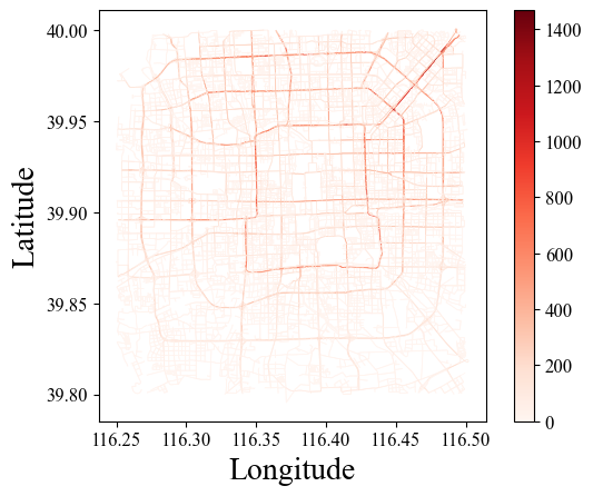
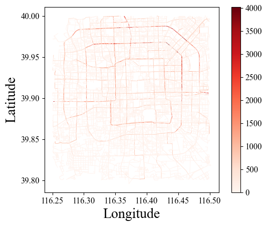
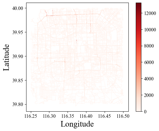
From the perspective of macro-similarity, compared with the second best model, TS-TrajGen improves the Distance, Radius, and Location Frequency metrics by 97.57%, 98.94% and 70.09% respectively in BJ-Taxi. As for the OD Flow metric, since we take both the origin and destination as input, TS-TrajGen achieve to completely restore the real OD flow state of the city. Among the baselines, TrajGen performs best because the trajectories it generates are derived from images, which enables it to generate continuous trajectories as the image resolution increases. While other sequential generative baselines fail to model the continuous mobility pattern. Besides, to better illustrate the detailed difference, we leverage heat map to visualize the location distribution of the top three generated data in Beijing, as shown in Figure 2.

As for the micro-similarity, our proposed TS-TrajGen achives to simulate the individual trajectory, and shows clear advantages over others, which is mainly because other baseline models ignore the impact of destination on the human mobility behavior.
Case Study
Case Study 1: Trajectory Next-Location Prediction.
Trajectory next-location prediction task aims to predict the location of mobility trajectory through mining the human mobility patterns. Therefore, we can leverage this task to examine whether there are real mobility patterns in the generated data based on BJ-Taxi dataset.
In this case study, we choose DeepMove (Feng et al. 2018) as the trajectory next-location prediction model. We mix the generated data with the real data in various ratios and train the DeepMove model using the mixed data. Then, we test the model performance on real data and calculate the performance difference from the model trained entirely on real data.
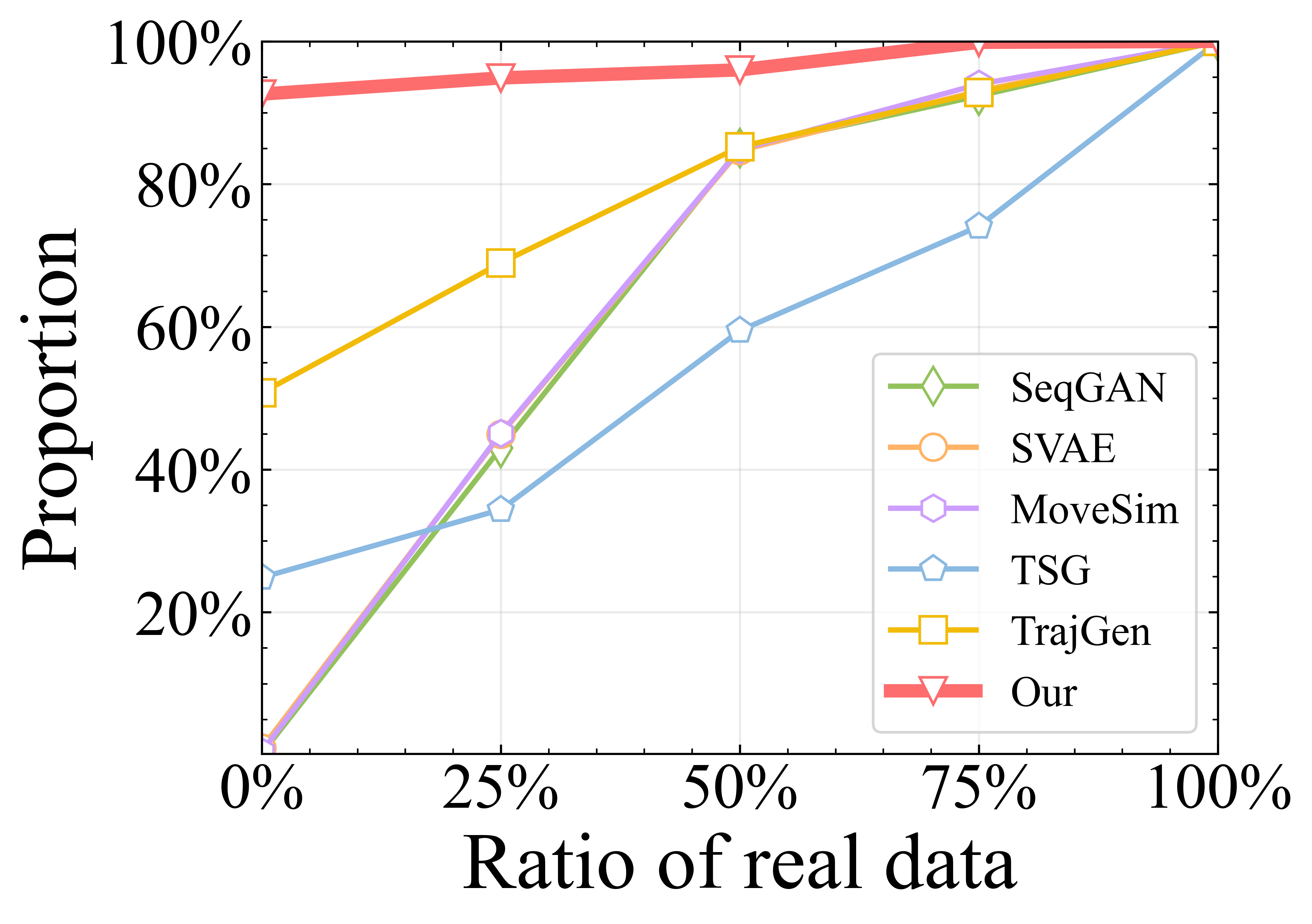
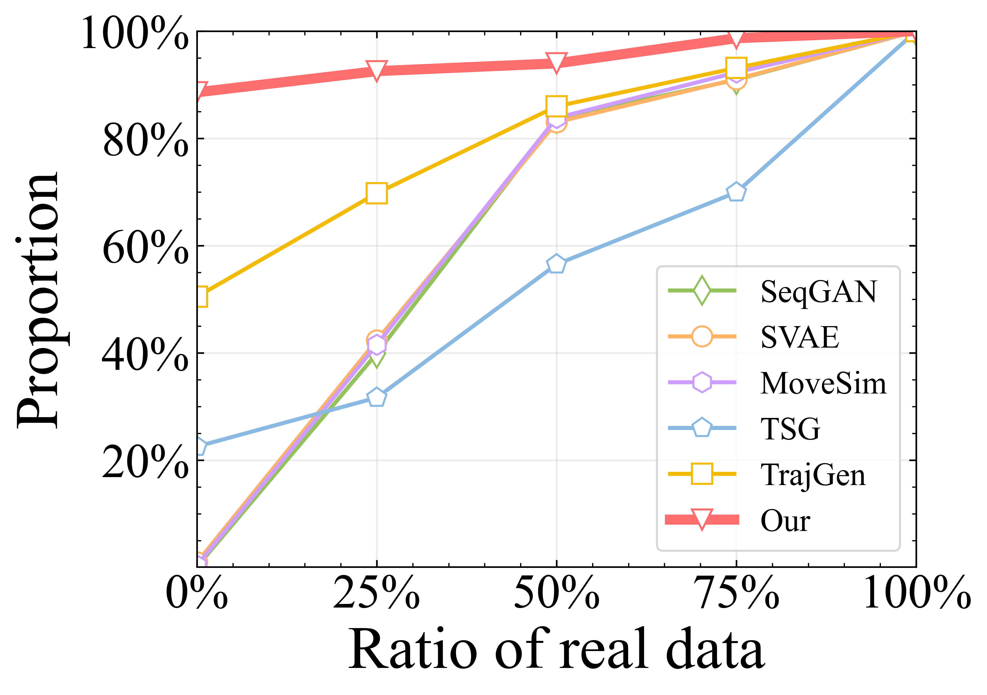
Figure 3 shows the performance difference between the model trained on the mixed data and the model trained on the real data, e.g., only the real data is used for training when the value is 100%. We can conclude the utility of our generated data exceeds the data generated by other models. When only trained with our generated data, the DeepMove achieves 92.61% and 88.59% performance of the DeepMove trained on real data on the Recall@5 and NDCG@5 metrics respectively. However, among the baselines, the best proportions of performance are 50.74% and 50.47% respectively.
Case Study 2: Traffic Control Simulation.
Traffic simulation is an important application of trajectory generation. Thus, we choose a case of Beijing Sanyuan Bridge traffic control to verify that our framework is competent for the human mobility simulation task.
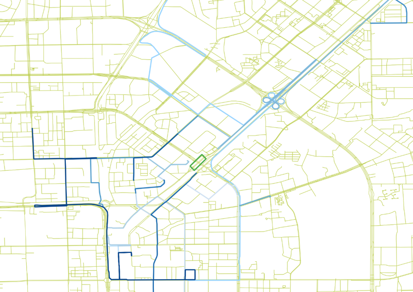
On November 13, 2015, the Sanyuan Bridge on the Third Ring Road in Beijing was imposed a one-day traffic control due to the construction reason. We randomly visualized 15 trajectories without and with traffic control near the Sanyuan Bridge, as shown in Figure 4(a) and Figure 4(b), where the green lines are the Beijing road network, the blue lines are the trajectories of different vehicles, and the area in the green box is the Sanyuan Bridge.
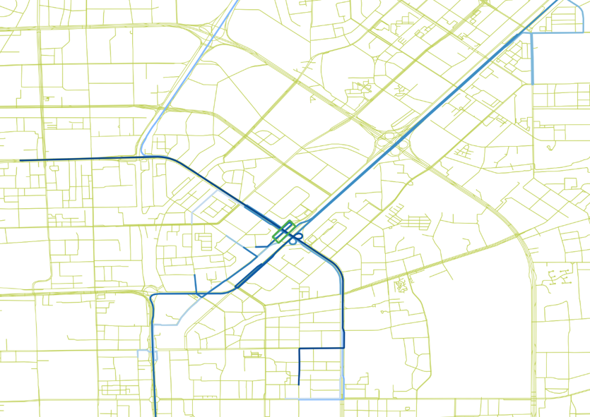
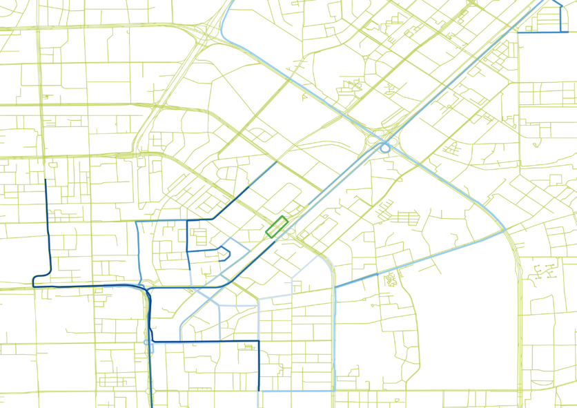
In this case study, we set the roads under construction as unreachable and then simulate trajectories nearby Sanyuan Bridge. The part of simulation result is visualized in Figure 4(c). In addition, we quantitatively calculate the micro similarity between real trajectories and generated trajectories. However, since none of the above baseline models can handle the traffic control situation, we chose two route planning models as baseline models in this case study, i.e., NASR(Wang et al. 2019) and A* search(Hart, Nilsson, and Raphael 1968). The evaluation result is shown in Table 3. From the test result, our TS-TrajGen is closer to the real traffic control situation than existing route planning method NASR, and achieves significant progress on the first two metrics.
| Hausdorff | DTW | EDR | |
|---|---|---|---|
| A* search | 2.7599 | 49.3791 | 0.7160 |
| NASR | 2.0393 | 37.1353 | 0.5658 |
| Our | 0.9790 | 16.3914 | 0.5451 |
Related Work
The trajectory generation problem takes an origin road segment and an destination road segment as input, and outputs the corresponding trajectory. Existing works of trajectory generation can be classified into two groups: model-based methods and model-free methods. Based on assumptions about the human mobility regularity, model-based methods model the individual mobility by limited parameters. For example, TimeGeo (Jiang et al. 2016) leverages data-driven methods to estimate the parameters from the real data, and then generate trajectory via Markov based models with the simplified assumption of human mobility. While achieving promising performance in some cases, these methods with simplified assumptions can not model the complex mobility in reality.
Recently, the researchers turned to apply model-free methods like VAE and GAN to generate the mobility trajectory. SAVE (Huang et al. 2019) is a combination of VAE and Seq2Seq model, which combines the ability of VAE to learn the underlying distribution of real data and the ability of LSTM to process sequential data. MoveSim (Feng et al. 2020) is a model-free GAN framework that integrates the domain knowledge of human mobility regularity. TrajGen (Cao and Li 2021) maps a trajectory into an image and utilizes a CNN-based GAN to generate the virtual trajectory image. Then, TrajGen applies a Seq2Seq model to infer the real trajectory sequence from the location sequence extracted from the virtual image. Although these methods do not rely on the simplified human mobility assumptions, but instead directly learned the underlying distribution of the data. However, these methods igonre the problem of the continuity of the generated trajectory, which is crucial in practical human mobility simulation applications. Hence, we propose a novel two-stage generative adversarial framework to solve this problem.
Conclusion
In this paper, we propose a novel two-stage generative adversarial framework to solve the continuous trajectory generation problem, which combines the advantages of human mobility prior knowledge with the model-free learning paradigm. Although many previous works have investigated the trajectory generation problem, we are the first to directly generate continuous trajectories on the road network. The extensive experiments demonstrate that our framework outperforms five state-of-the-art baselines significantly, including aspects of macro-similarity, micro-similarity and data utility. Besides, through a traffic control simulation case study, we prove that our framework can be directly applied to real-world city traffic simulations. As future work, we will further explore other potential factors of human mobility and extend the simulation to various applications.
Acknowledgments
This work was supported by the National Key R&D Program of China (2021ZD0111201). Prof. Wang’s work was supported by the National Natural Science Foundation of China (No. 82161148011, 72222022, 72171013), the Fundamental Research Funds for the Central Universities (YWF-22-L-838) and the DiDi Gaia Collaborative Research Funds. Prof. Zhao’s work was supported by the National Natural Science Foundation of China (No. 62222215).
References
- Brockmann, Hufnagel, and Geisel (2006) Brockmann, D.; Hufnagel, L.; and Geisel, T. 2006. The scaling laws of human travel. Nature, 439(7075): 462–465.
- Cao and Li (2021) Cao, C.; and Li, M. 2021. Generating Mobility Trajectories with Retained Data Utility. In Proceedings of the 27th ACM SIGKDD Conference on Knowledge Discovery and Data Mining, KDD ’21, 2610–2620. New York, NY, USA: Association for Computing Machinery. ISBN 9781450383325.
- Chen, Özsu, and Oria (2005) Chen, L.; Özsu, M. T.; and Oria, V. 2005. Robust and Fast Similarity Search for Moving Object Trajectories. In Proceedings of the 2005 ACM SIGMOD International Conference on Management of Data, SIGMOD ’05, 491–502. New York, NY, USA: Association for Computing Machinery. ISBN 1595930604.
- Feng et al. (2018) Feng, J.; Li, Y.; Zhang, C.; Sun, F.; Meng, F.; Guo, A.; and Jin, D. 2018. DeepMove: Predicting Human Mobility with Attentional Recurrent Networks. In Proceedings of the 2018 World Wide Web Conference, WWW ’18, 1459–1468. Republic and Canton of Geneva, CHE: International World Wide Web Conferences Steering Committee. ISBN 9781450356398.
- Feng et al. (2020) Feng, J.; Yang, Z.; Xu, F.; Yu, H.; Wang, M.; and Li, Y. 2020. Learning to Simulate Human Mobility. In Proceedings of the 26th ACM SIGKDD International Conference on Knowledge Discovery and Data Mining, KDD ’20, 3426–3433. New York, NY, USA: Association for Computing Machinery. ISBN 9781450379984.
- González, Hidalgo, and Barabási (2008) González, M. C.; Hidalgo, C. A.; and Barabási, A. 2008. Understanding individual human mobility patterns. nature, 453(7196): 779–782.
- Hart, Nilsson, and Raphael (1968) Hart, P. E.; Nilsson, N. J.; and Raphael, B. 1968. A Formal Basis for the Heuristic Determination of Minimum Cost Paths. IEEE Transactions on Systems Science and Cybernetics, 4(2): 100–107.
- Hochreiter and Schmidhuber (1997) Hochreiter, S.; and Schmidhuber, J. 1997. Long Short-Term Memory. Neural Comput., 9(8): 1735–1780.
- Huang et al. (2019) Huang, D.; Song, X.; Fan, Z.; Jiang, R.; Shibasaki, R.; Zhang, Y.; Wang, H.; and Kato, Y. 2019. A Variational Autoencoder Based Generative Model of Urban Human Mobility. In 2019 IEEE Conference on Multimedia Information Processing and Retrieval (MIPR), 425–430.
- Jiang et al. (2016) Jiang, S.; Yang, Y.; Gupta, S.; Veneziano, D.; Athavale, S.; and González, M. C. 2016. The TimeGeo modeling framework for urban mobility without travel surveys. Proceedings of the National Academy of Sciences, 113(37): E5370–E5378.
- Keogh (2002) Keogh, E. 2002. Chapter 36 - Exact Indexing of Dynamic Time Warping. In Bernstein, P. A.; Ioannidis, Y. E.; Ramakrishnan, R.; and Papadias, D., eds., VLDB ’02: Proceedings of the 28th International Conference on Very Large Databases, 406–417. San Francisco: Morgan Kaufmann. ISBN 978-1-55860-869-6.
- Luca et al. (2021) Luca, M.; Barlacchi, G.; Lepri, B.; and Pappalardo, L. 2021. A Survey on Deep Learning for Human Mobility. ACM Comput. Surv., 55(1).
- Ouyang et al. (2018) Ouyang, K.; Shokri, R.; Rosenblum, D. S.; and Yang, W. 2018. A Non-Parametric Generative Model for Human Trajectories. In Proceedings of the Twenty-Seventh International Joint Conference on Artificial Intelligence, IJCAI-18, 3812–3817. International Joint Conferences on Artificial Intelligence Organization.
- Paola et al. (2019) Paola, A. D.; Giammanco, A.; Re, G. L.; and Morana, M. 2019. Human Mobility Simulator for Smart Applications. In 2019 IEEE/ACM 23rd International Symposium on Distributed Simulation and Real Time Applications (DS-RT), 1–8.
- Pellungrini et al. (2017) Pellungrini, R.; Pappalardo, L.; Pratesi, F.; and Monreale, A. 2017. A Data Mining Approach to Assess Privacy Risk in Human Mobility Data. ACM Trans. Intell. Syst. Technol., 9(3).
- Sanders and Schulz (2013) Sanders, P.; and Schulz, C. 2013. Think Locally, Act Globally: Highly Balanced Graph Partitioning. In Proceedings of the 12th International Symposium on Experimental Algorithms (SEA’13), volume 7933 of LNCS, 164–175. Springer.
- Simini et al. (2012) Simini, F.; González, M. C.; Maritan, A.; and Barabási, A.-L. 2012. A universal model for mobility and migration patterns. Nature, 484(7392): 96–100.
- Song et al. (2010) Song, C.; Koren, T.; Wang, P.; and Barabási, A.-L. 2010. Modelling the scaling properties of human mobility. Nature physics, 6(10): 818–823.
- Vaswani et al. (2017) Vaswani, A.; Shazeer, N.; Parmar, N.; Uszkoreit, J.; Jones, L.; Gomez, A. N.; Kaiser, L. u.; and Polosukhin, I. 2017. Attention is All you Need. In Guyon, I.; Luxburg, U. V.; Bengio, S.; Wallach, H.; Fergus, R.; Vishwanathan, S.; and Garnett, R., eds., Advances in Neural Information Processing Systems, volume 30. Curran Associates, Inc.
- Veličković et al. (2018) Veličković, P.; Cucurull, G.; Casanova, A.; Romero, A.; Liò, P.; and Bengio, Y. 2018. Graph Attention Networks. In International Conference on Learning Representations.
- Wang et al. (2021a) Wang, J.; Jiang, J.; Jiang, W.; Li, C.; and Zhao, W. X. 2021a. LibCity: An Open Library for Traffic Prediction. In Proceedings of the 29th International Conference on Advances in Geographic Information Systems, SIGSPATIAL ’21, 145–148. New York, NY, USA: Association for Computing Machinery. ISBN 9781450386647.
- Wang et al. (2019) Wang, J.; Wu, N.; Zhao, W. X.; Peng, F.; and Lin, X. 2019. Empowering A* Search Algorithms with Neural Networks for Personalized Route Recommendation. In Proceedings of the 25th ACM SIGKDD International Conference on Knowledge Discovery and Data Mining, KDD ’19, 539–547. New York, NY, USA: Association for Computing Machinery. ISBN 9781450362016.
- Wang et al. (2021b) Wang, X.; Liu, X.; Lu, Z.; and Yang, H. 2021b. Large Scale GPS Trajectory Generation Using Map Based on Two Stage GAN. Journal of Data Science, 19(1): 126–141.
- Williams (1992) Williams, R. J. 1992. Simple statistical gradient-following algorithms for connectionist reinforcement learning. Machine learning, 8(3): 229–256.
- Xie, Li, and Phillips (2017) Xie, D.; Li, F.; and Phillips, J. M. 2017. Distributed Trajectory Similarity Search. Proc. VLDB Endow., 10(11): 1478–1489.
- Yang and Gidofalvi (2018) Yang, C.; and Gidofalvi, G. 2018. Fast map matching, an algorithm integrating hidden Markov model with precomputation. International Journal of Geographical Information Science, 32(3): 547–570.
- Yin, Yang, and Ma (2018) Yin, D.; Yang, Q.; and Ma, L. 2018. GANs Based Density Distribution Privacy-Preservation on Mobility Data. Sec. and Commun. Netw., 2018.
- Yu et al. (2017) Yu, L.; Zhang, W.; Wang, J.; and Yu, Y. 2017. SeqGAN: Sequence Generative Adversarial Nets with Policy Gradient. In Proceedings of the Thirty-First AAAI Conference on Artificial Intelligence, AAAI’17, 2852–2858. AAAI Press.