A continuum limit for dense networks

Abstract

Differential equations on metric graphs model disparate phenomena, including electron localisation in semiconductors, low-energy states of organic molecules, random laser networks, pollution diffusion in cities, dense neuronal networks and vasculature. This article describes the continuum limit of the edgewise Laplace operator on metric graphs, where vertices fill a given space densely, and the edge lengths shrink to zero (e.g. a spider web filling in a unit disc). We derive a new, coarse-grained partial differential operator which depends on the embedding space and local graph structure and has interesting similarities and differences with the Riemannian Laplace-Beltrami operator. We highlight various subtleties of dense metric graph systems with several semi- and fully analytic examples.

In this paper, we report a new kind of macroscopic medium which emerges systematically from a dense network of interconnected “wires” or “conduits”. The mathematical notion of a discrete graph dates back to Euler’s 1726 solution of the Seven Bridges of Königsberg problem, abstracting the city’s street network to a discrete collection of pairwise relations between nodes. But perhaps a more overt definition would “address” the thoroughfares as contiguous physical connections between junctions. In this case, the appropriate structure is a “metric graph” a.k.a. “geometrised network” a.k.a. “continuous graph”: a discrete graph with physical length along each edge. A significant advantage of metric graphs over their discrete counterparts is that they support the imposition of differential equations along their edges.

Metric graphs are ubiquitous: optical fibre networks, electrical power grids, spider webs, vasculature, river systems, neuronal networks, textiles, fishing nets, or British Rail. Moreover, metric graphs find application in diverse and less obvious abstract settings, for example: microwave lattices, quantum chemistry, and dynamical systems theory.

We embed a metric graph within some common space (e.g. a smooth manifold such has Euclidean space or the 2-sphere). We pose a typical dynamical model as a one-dimensional differential equation on each edge, with “boundary” conditions at each vertex. Overall, the dynamics on a given edge depend on the dynamics over the entire graph. In this sense, we envision a kind of “mesoscopic” system giving way to fully coarse-grained dynamics. The overall question we address is:

What partial differential equations result from taking the “continuum limit” of the metric graph, where the vertices become dense in the embedding space, and the edge lengths shrink to zero (figure 1a)?

We answer this question for the eigensystem of the Laplace operator $\Delta=d^{2}/dx^{2}$ 1 on each edge of a given metric graph $G$, and find the resulting PDE is (11). We chose the differential Laplacian as a starting point because of its presence in innumerable applications.

There has been significant work studying differential equations on metric graphs, mainly focusing on quantum Hamiltonian Schrödinger operators, $\mathcal{H}=-\Delta+V(x)$ [1]. Linus Pauling first considered differential equations on metric graphs to model free electrons in organic molecules [2]. Recent modelling efforts include: Hamiltonian dynamics in hydrocarbons [3, 4, 5, 6] and low-energy eigenmodes of protonated methane [7, 8] using similar, 60 vertex models to the truncated icosahedron (buckminsterfullerene) in figure 1d. Particular excitement exists regarding nanomaterials for their remarkable mechanical, electric and optical properties [9, 10, 11, 12, 13, 14, 15, 16, 17]. The Schrödinger equation on metric graphs is also equivalent to the telegraph equation on microwave networks [18, 19, 20, 21, 22]. Localisation landscape theory provides a promising model for charge-carrier dynamics in disordered semiconductors [23, 24, 25, 26, 27, 28]. Anderson localisation has been studied extensively on quantum graphs [29, 30, 31, 32, 33]; including in random laser networks [34, 35, 36, 37, 38].

For biological applications, the brain presents an especially intriguing setting for high-density graph models [39, 40, 41, 42, 43, 44, 45, 46, 47, 48]. However, comparatively little work has included Euclidean distances on the underlying graphs; only how distance affects neuron firing rate synchronisation [49, 50]. The cellular cytoskeleton network of protein filaments is another key area for metric graph applications [51, 52, 53, 54, 55].

Mathematical results for differential equations on metric graphs include hybrid monographs covering the nonlinear Schrödinger and reaction-diffusion equations [56, 57, 58]. Other examples include thin-branched structures [59, 60], control problems [61], and semigroup methods for evolution equations [62]. A related work [63] demonstrates how a discrete lattice of wires is nevertheless able to efficiently filter electromagnetic radiation as would a continuous substance. Lieb et al. solve and optimise a system of nonlinear conservation laws on idealised urban water-supply networks [64].

Little is understood regarding high-density (continuum-limit) metric graphs as embedded structures within manifolds. Previous work treats graphs with high levels of symmetry [65, 66, 1, 67, 68, 69, 70, 71, 72]. Applications exist in the human circulatory system [73, 74], population dynamics [75], tissue membranes [76] and urban pollution [77]. Lastly, [78] shows Ollivier-to-Ricci curvature convergence for edges with positive weights.

Mathematical setup

A metric graph $G=(V,\,E)$ is a collection of vertices, $V$, and edges, $E$, with local Euclidean coordinates on each edge $x\in[0_{e},\ell_{e}]\simeq{e}\in{E}$. The parameterised edges of a metric graph embedded within a manifold need not be straight; a balled-up fishing net is the same as its laid-flat counterpart.

A real-valued scalar function, $f(e,x)$ for $x\in{e}$, is globally continuous if it is continuous on all individual edges and single-valued on all vertices. Defining differentiability is more subtle. Even infinitely smooth functions along each edge frequently disagree at the vertices, which is, in fact, “a feature, not a bug”.

We consider the local edgewise Laplace eigenvalue equation,

$$\frac{d^{2}}{dx^{2}}f(e,x)\ =\ -k^{2}f(e,x).$$ (1)

The Kirchhoff condition,

$$\sum_{e\sim v}\hat{B}_{ve}\,\frac{d}{dx}f(e,x)\Big{|}_{x=v}\ =\ 0,$$ (2)

where $\hat{B}_{ve}=\pm{1}$ is the unit normal outward from edge-$e$ at vertex $v$ (supplemental material (SM) [79]). The Kirchhoff condition (2) shows why relevant functions often have multi-valued derivatives at vertices. The spectrum $\lambda=-k^{2}$ is real-valued and discrete [1] and could represent (e.g.) the spatial component of heat diffusion ($\partial_{t}\to-k^{2}$), wave-like dynamics ($\partial_{t}^{2}\to-k^{2}$), or Schrödinger evolution ($-i\partial_{t}\to-k^{2}$).

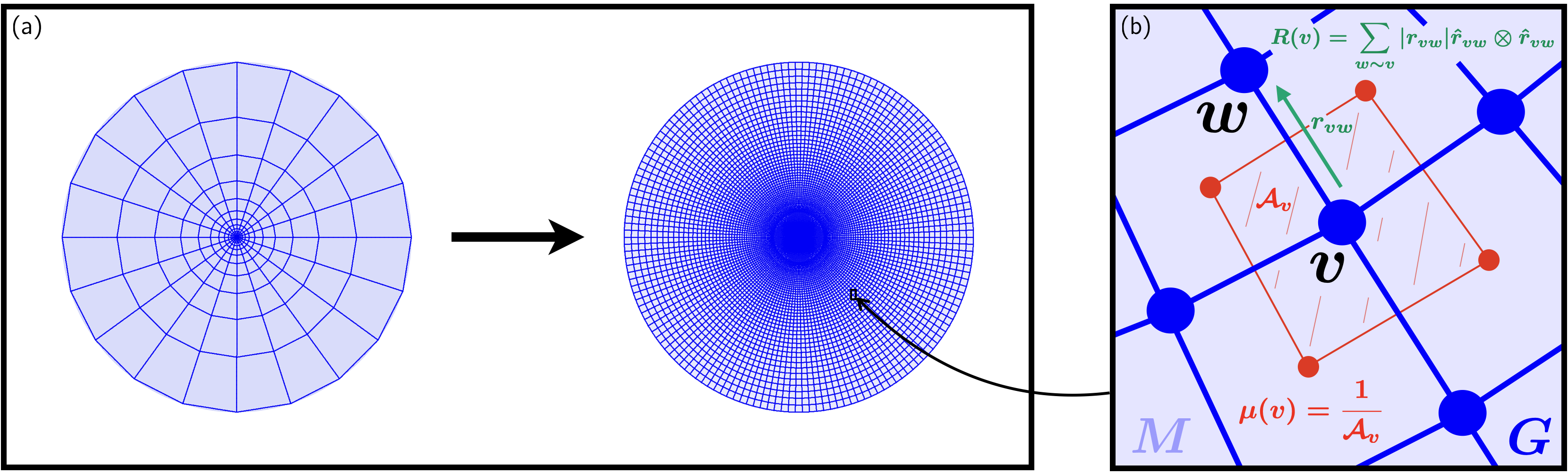
Figure 1: a) The continuum limiting procedure for the spiderweb within the unit disc. b) PDE quantities: the edge tensor $R$ (8), and the vertex density $\mu$ (7).

If a given edge $e$ has endpoints $v\simeq 0_{e}$, $w\simeq\ell_{e}$, then from (1),

$$f(e,x)\ =\ f(v)\,\frac{\sin(k(\ell_{e}-x))}{\sin(k\ell_{e})}+f(w)\,\frac{\sin(kx)}{\sin(k\ell_{e})},$$ (3)

which manifestly expresses continuity, $f(e,0_{e})=f(v)$, $f(e,\ell_{e})=f(w)$. The vertex Kirchhoff condition at vertex $v$ is

$$k\sum_{w\sim v}\csc(k\ell_{vw})\,f(w)-\cot(k\ell_{vw})f(v)\ =\ 0,$$ (4)

a finite algebraic system over $V$, $L(k)\cdot{f_{V}}=0$. The spectral condition is $\det(L(k))=0$, which we solve numerically for $k,\,f_{V}$ (see SM [79]). Finally (4) derives from the 1st-order stationarity of the finite quadratic functional,

$$Q(f)\ =\ k\sum_{v}\sum_{w\sim v}\left\{\cot(k\ell_{vw})\left(f(v)-f(w)\right)^{2}\hskip 8.5359pt\right.$$

$$\left.-2\tan\left(\tfrac{1}{2}k\ell_{vw}\right)f(v)f(w)\right\}.$$ (5)

Continuum limit

We embed our metric-graph solution in a general Riemannian manifold $M\supset{G}$. The vertices simply are points $v\in{M}$. The edges are either fully embedded, $e\subset{M}$, or could be straight chords embedded within a higher-dimensional Euclidean space. In the continuum limit, both options will give the same result: for any two adjacent vertices, $w\sim{v}$, we take the limit as $\ell_{vw}\to 0$ but allow the number of vertices to fill in densely in $M$.

We assume $M$ has a Riemannian structure with a natural volume measure. However, our eventual results are independent of a particular underlying Riemannian metric. The graph requires a vertex number density, $\mu(x)$, such that for all sufficiently coarse-grained subsets $S\subseteq{G}$,

$$\int_{S}\mu(x)\,\text{d}{x}\ =\ \text{number vertices}\in S.$$ (6)

The function, $\mu(x)$, is the Radon-Nikodym derivative with respect to the geometric measure on the manifold. Trivially, we can use the empirical measure on the vertices $\mu_{V}(x)=\sum_{v\in V}\delta(x-x_{v})$. The empirical measure converges weakly to a continuum limit as the graph becomes dense. For an orthonormal basis of square-integrable functions $\psi_{k}(x)\in\mathcal{L}^{2}(G)$,

$$\mu_{N}(x)\ =\ \sum_{k\leq N}\psi_{k}(x)\sum_{v\in V}\psi_{k}(x_{v})\ \approx\ \frac{1}{|\mathcal{A}_{v}|},$$ (7)

for $x\in\mathcal{A}_{v}$, the dual cell area (volume in general) surrounding a given vertex (see figure 1b). The spectral representation approximates the empirical measure for functions of bounded variation, which is also sufficient to define the weak derivative [80].

We derive a formal continuum limit $\ell_{vw}\to 0$. First, $k\cot(k\ell_{vw})\sim 1/\ell_{vw}$ and $2k\tan(\tfrac{1}{2}k\ell_{vw})\sim{k^{2}}\ell_{vw}$. Then $f(w)-f(v)\sim{r_{vw}}\cdot\nabla{f(v)}$ as $|r_{vw}|=\ell_{vw}\to 0$ with $\hat{r}_{vw}=r_{vw}/|r_{vw}|$ pointing from $v$ to $w$ along their common edge.

Now comes the crux of the derivation. We define the following graph “edge” tensor at each vertex (see figure 1b)

$$R(v) \!\!\!= \!\!\!\sum_{w\sim v}|r_{vw}|\,\hat{r}_{vw}\otimes\hat{r}_{vw},$$ (8)

$$\text{tr}\!\left({R(v)}\right) \!\!\!= \!\!\!\sum_{w\sim v}|r_{vw}|,$$ (9)

where $\hat{r}_{vw}\cdot\hat{r}_{vw}=1$. Therefore, to $\mathcal{O}(\ell_{vw}^{2})$,

$$Q(f)\ =\ \int_{G}\left[\nabla f(x)\cdot R(x)\cdot\nabla f(x)\right.-\hskip 14.22636pt$$

$$\left.k^{2}\,\text{tr}\!\left({R(x)}\right)f(x)^{2}\right]\mu(x)\,\text{d}{x}.$$ (10)

Computing the variational derivative of the continuum functional produces the eigenvalue problem in the dense limit:

$$\frac{1}{\mu\,\text{tr}\!\left({R}\right)}\nabla\cdot\left(\mu\,R\cdot\nabla f\right)\ =\ -k^{2}f,$$ (11)

for $x\in G$. The associated “natural” boundary conditions are

$$\hat{n}\cdot R\cdot\nabla f=0\quad\text{for}\quad x\in\partial G,$$ (12)

where $\hat{n}$ is the unit normal to the boundary. Alternatively, $f(x)=0$ for pinned boundary vertices.

Tensor comparisons

Nematic comparison

The edge tensor is analogous to other examples appearing in diverse applications but with a different inverse length scaling. Generalising the summand, $q_{vw}^{(\alpha)}=|r_{vw}|^{\alpha}\,r_{vw}\otimes\,r_{vw}$, with $R(v)$ corresponding to $\alpha=-1$. For $\alpha=0$, the conformation (a.k.a neumatic-order) tensor, $Q$, gives the degree of alignment in liquid crystals [81],

$$Q(v)\ \propto\ \sum_{w}\left(q_{vw}^{(0)}-\frac{1}{d}\,\text{tr}\!\left({q_{vw}^{(0)}}\right)\,I\right),$$ (13)

so that $\text{tr}\!\left({Q}\right)=0$ by definition. An isotropic material implies $Q=0$. For a perfect nematic $Q$ is a diagonal matrix.

Riemannian comparison

The inverse Riemannian metric tensor roughly corresponds to $\alpha=-2$. The reduced system resembles the standard Laplace-Beltrami operator on a manifold with an augmented local metric tensor, $g(x)$. However, there is no clear way to put (11) into one-to-one correspondence with an Laplace-Beltrami operator, even if we impose conditions on the type of Riemannian metric. The edge tensor is defined similarly to a discrete approximation of a Riemannian metric, but with a different distance scaling, i.e., with closest correspondence (see SM [79])

$$g(v)^{-1}\ \longleftrightarrow\ \frac{\text{dim}(M)}{\text{deg}(v)}\sum_{w\sim v}\hat{r}_{vw}\otimes\hat{r}_{vw}.$$ (14)

For Riemannian metrics, $\text{tr}\!\left({g}\right)=\text{dim}(M)$ by definition. As far as we know, there is no straightforward way to relate $R$ to any other standard tensors commonly defined on Riemannian manifolds. Moreover, the local Riemannian volume measure is $\sqrt{\det(g)}$. There appears to be no simple procedure to obtain the vertex density, $\mu(x)$, in terms of a function of $R(x)$ alone. The underlying presence of a metric graph “substance” cannot be described purely in geometrical terms.

We can see that the (11) gives genuinely distinct behaviour from a traditional Laplace-Beltrami operator, with the main differences resulting from the trace, $\text{tr}\!\left({R}\right)$. For a completely homogeneous isotropic graph, the only symmetric rank-2 tensor is proportional to the $d$-dimensional identity,

$$R\ =\ \frac{\text{tr}\!\left({R}\right)}{d}\,I_{d}\quad\implies\quad\frac{1}{d}\,\Delta f\ =\ -k^{2}f.$$ (15)

For rectangular lattice, [77] finds a medium-range diffusion kernel based on the squared Manhattan distance, $||x||_{1}$ rather than the rotationally invariant Euclidean metric, $||x||_{2}$. However, the general bound $||x||_{1}^{2}\leq{d}\,||x||_{2}^{2}$ implies the results accord in the full continuum limit.

Isotropy implies $\text{tr}\!\left({R}\right)=\ell\,\deg(v)$ is constant for every vertex. For this special case, (11) reduces to the standard Laplace-Beltrami operator, but weighted by the spatial dimension of the graph embedding. Overall, the continuum “graph material” can resemble many other materials but is (roughly speaking) less stiff by the dimension of the embedding space. On perfectly square lattices [82, 83, 84, 85] rigorously prove formal operator convergence to (15), particularly commenting about the anomalous dimensional factor.

Exact and numerical comparisons

Periodic planar torus

We confirm (15) with a series of simple, exactly solvable graph models and take the large-scale limit directly.

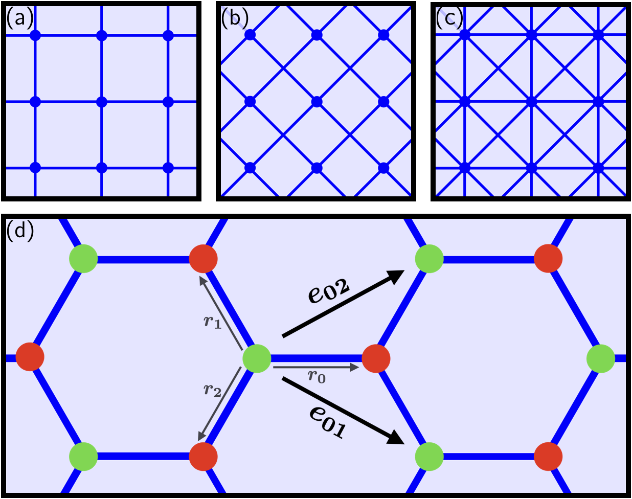
Figure 2: The periodic lattices present analytically solvable examples in both the metric graph and PDE cases. Dispersion relations for (a)-(c) cardinal, ordinal, and both connections are immediate. For the hexagonal lattice, the vectors $e_{01}=r_{0}-r_{1}$ and $e_{02}=r_{0}-r_{2}$ quantise the dispersion relation (20).

The Kirchhoff vertex condition (2) simplifies considerably for uniform edge lengths,

$$\cos(k\ell)f(v)-\frac{1}{\text{deg}(v)}\sum_{w\sim v}f(w)\ =\ 0.$$ (16)

If $e_{1},e_{2}\in\mathbb{R}^{2}$ are fundamental lattice vectors the periodicity implies $f(x+N_{j}\,e_{j})=f(x)$ for sufficiently large integers $N_{j}$. For plane-wave solutions,

$$f(x)\ =\ A\,e^{i\,a\cdot x}+\text{c.c.},\quad a=\sum_{j}a_{j}\,\tilde{e}_{j},$$ (17)

with dual vectors $\tilde{e}_{i}\cdot{e_{j}}=\ell\,\delta_{i,j}$ and quantised components $a_{j}=2\pi\,n_{j}/N_{j}$.

For cardinal (N-S-E-W), ordinal (NE-SW-SE-NW) connectivities (figures 2a-b), the dispersion relations are,

$$\cos(k\ell) = \frac{1}{2}\left(\cos(a_{1}\ell)+\cos(a_{2}\ell)\right),$$ (18)

$$\cos(\sqrt{2}k\ell) = \cos(a_{1}\ell)\cos(a_{2}\ell)$$ (19)

The dispersion relation for the combined lattice (figure 2c) is a simple sum of (18) and (19), each weighted by $\csc(k\ell)$ and $\csc(\sqrt{2}k\ell)$ respectively.

The ordinal-case dispersion relation is particularly intriguing: (19) is the Pythagorean Theorem for a right triangle on the surface of a sphere with spherical angles $a_{1}\ell,\,a_{2}\ell$ and $\sqrt{2}k\ell$. The cardinal-case (18) is equivalent to a spherical Pythagorean theorem only rotated by $45^{\circ}$. We note that nontrivial geometric structure in spectral space can lead to (e.g.) symmetry-induced topological protection [86].

For hexagonal connectivity figure 2d highlights two disjoint sets of coupled vertices: “green” with neighbours at $r_{j}=\ell\left(\cos\left(\tfrac{2\pi}{3}j\right),\sin\left(\tfrac{2\pi}{3}j\right)\right)$ for $j=0,1,2$, and “red” with neighbours $-r_{j}$. Since neither colour group contains both $\pm{r_{j}}$ edges, we cannot substitute simple plane wave solutions into (16) and automatically obtain a real-valued dispersion relation. However, applying the Kirchhoff condition twice yields

$$\cos^{2}(k\ell)\ =\ \frac{1}{9}\bigg{(}3+2\sum_{i<j}\cos(a\cdot(r_{i}-r_{j})\bigg{)},$$ (20)

where $e_{i,j}=r_{i}-r_{j}$ are lattice vectors such that

$$\sum_{i<j}e_{i,j}\otimes e_{i,j}\ =\ \frac{9\ell^{2}}{2}I_{2}.$$ (21)

A spherical triangle automatically reduces to a Cartesian triangle as $\ell\to 0$, and (18) is simply a rotated version of (19). The relation for cardinal + ordinal connectivity is simply a combination of the two (SM [79]). In all cases,

$$k^{2}\ =\ \frac{a\cdot a}{d}\ +\ \mathcal{O}(\ell^{2})\quad\text{as}\quad\ell\to 0.$$ (22)

with $d=2$, corresponding to (15). The same relation holds for higher-dimensional lattices. For a rectangular lattice with anisotropic edge lengths, $R$ contains unequal diagonal entries and therefore,

$$\left(\alpha\,\partial_{x}^{2}+(1-\alpha)\,\partial_{y}^{2}\right)f(x)\ =\ -k^{2}f(x),$$ (23)

where $\alpha=R_{xx}/(R_{xx}+R_{yy})$.

Inhomogeneous, anisotropic spiderweb

An axisymmetric “spiderweb” (figure 1a) provides a straightforward inhomogeneous anisotropic semi-analytic example. The spiderweb has local vertex spacings $\,\text{d}{r}$, $\,\text{d}{\theta}$ in each polar-coordinate direction $r$, $\theta$. It has a central vertex at the origin, boundary vertices on the unit circle, and interior vertices otherwise–for a total of $|V|=(N_{r}-1)N_{\theta}+1$ where $N_{r},N_{\theta}$ are the numbers of vertices in the radial and angular directions. At interior vertices

$$R(r) = R_{rr}\,\hat{r}\otimes\hat{r}+R_{\theta\theta}\,\hat{\theta}\otimes\hat{\theta},$$ (24)

$$R_{rr} = 2\,\text{d}{r}+4\,r\sin^{3}\!\left(\!\frac{\,\text{d}{\theta}}{2}\right)\sim 2\,\text{d}{r},$$ (25)

$$R_{\theta\theta} = \frac{r\sin^{2}(\!\,\text{d}{\theta})}{\sin\left(\frac{\,\text{d}{\theta}}{2}\right)}\sim 2\,r\,\text{d}{\theta}.$$ (26)

The vertex density is $\mu=1/\mathcal{A}_{v}$ with vertex-cell area $\mathcal{A}_{v}\sim{r}\,\text{d}{r}\,\text{d}{\theta}$. The angular spacing is $\,\text{d}{\theta}=2\pi/N_{\theta}$. The radial spacing depends smoothly on $r$ such that $\rho(r)=\,\text{d}{r}/\,\text{d}\theta$. Angular symmetry allows Fourier solutions, $f(r,\theta)=f_{m}(r)e^{im\theta}+\text{c.c.}$ Putting everything together,

$$r\rho(r)f_{m}^{\prime\prime}(r)+\left[r(r+\rho(r))k^{2}-m^{2}\right]f_{m}(r)\ =\ 0.$$ (27)

We use pinned outer boundary conditions $f_{m}(r=1)=0$. For centre-point conditions, $f_{m}^{\prime}(r=0)=0$ if $m=0$ and $f_{m}(r=0)=0$ otherwise. No choice of $\rho(r)$ can render the above operator into a Riemannian metric-based Laplacian. The original graph problem (4) also simplifies into decoupled radial systems (SM [79]).

The specific form $\rho(r)=r/\gamma$ allows analytical Bessel-like solutions. For $m\neq 0$,

$$f_{j,m}(r)\propto\sqrt{r}J_{\nu}(\sqrt{1+\gamma}\,k_{j,m}r),\ \ \nu=\sqrt{\gamma\,m^{2}+\tfrac{1}{4}},$$ (28)

where $J_{\nu}$ is the non-integer-order regular Bessel function. The spectral parameter, $k_{j,m}=\zeta_{j,\nu}/\sqrt{1+\gamma}$, where $J_{\nu}(\zeta_{j,\nu})=0$. The $m=0$ solution uses the Neumann function,

$$f_{j,0}(r)\propto\cos(\sqrt{1+\gamma}\,k_{j,0}r),\;\;k_{j,0}\ =\ \frac{(j+\tfrac{1}{2})\pi}{\sqrt{1+\gamma}}.$$ (29)

Figures 3a-b show the convergence of the numerical graph solutions $(k,\,f)$ to the analytic PDE solutions $(\tilde{k},\,\tilde{f})$ for increasing $N_{r}$. Given the Fourier decomposition into one-dimensional radial modes, both cases are very efficient. Figures 3c-d show visual comparisons between the graph and (graph-restricted) PDE modes, respectively.

Truncated icosahedron

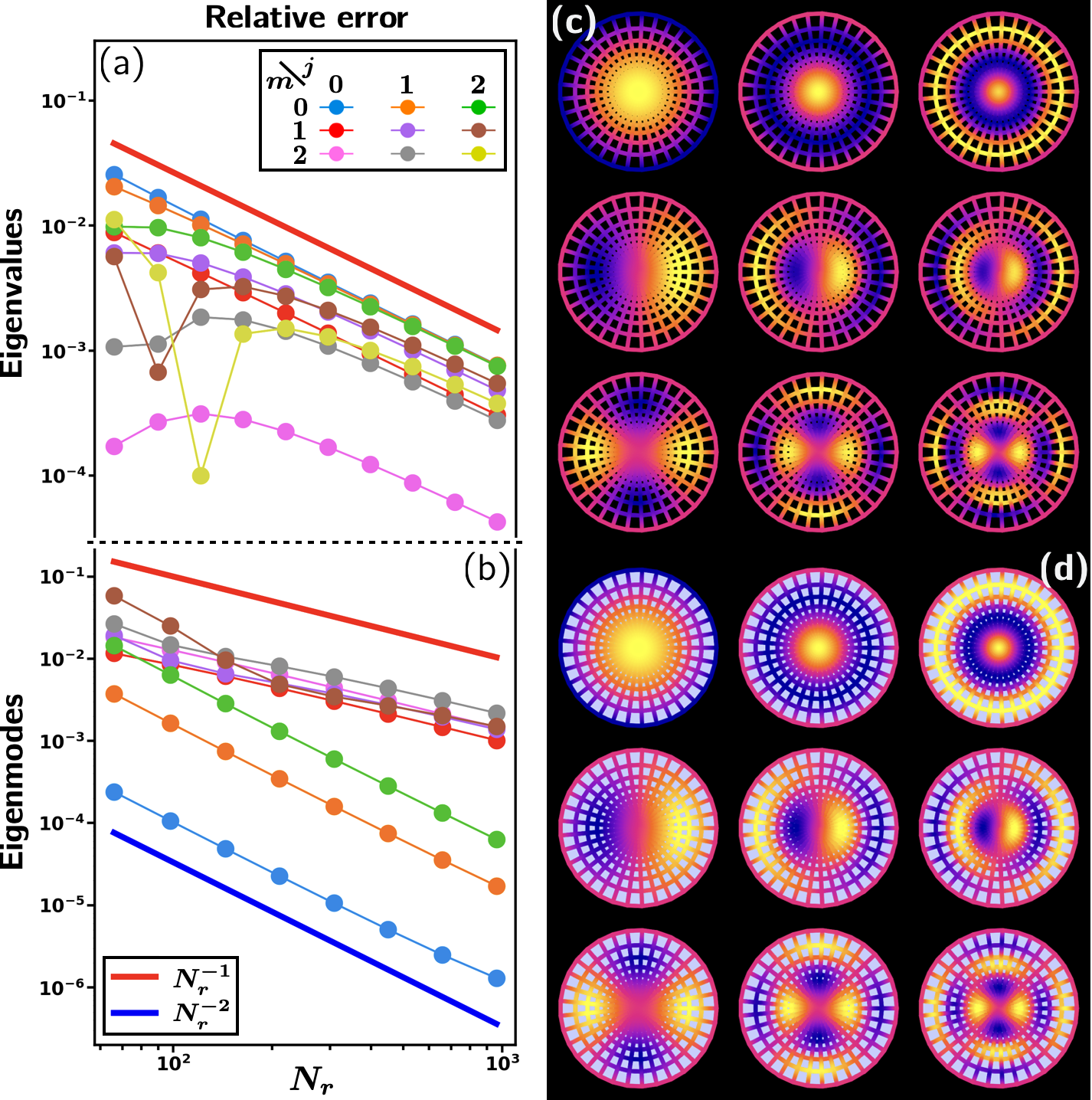
Figure 3: Continuum behaviour for dense spiderwebs — (a) & (b) Graph eigenvalues/eigenmodes converging to the PDE values (eqs. 28–29) for increasing numbers $N_{r}$ of radial vertices. (c) & (d) graph eigenmodes & graph-restricted PDE eigenmodes respectively for $(m,j)$ as per the legend of (a) for $|V|\approx 500$; both cases only show the angular cosine (and not sine) modes.

We demonstrate the continuum limit for curved surfaces with a truncated icosahedron (a.k.a. soccer ball or buckminsterfullerene, see figure 4a) embedded within the unit 2-sphere, $S^{2}$. While low-degree examples like the soccer ball have exact formulae for eigenvalues, any resulting PDE model will inevitably contain spatial inhomogeneities confounding exact solutions; the dodecahedron ($|V|=20$) is the largest regular tessellation of $S^{2}$. The soccer ball represents a simple enough intermediate case to provide analytical intuition. The point is that even relatively low-density metric graphs display continuum behaviour for low-degree eigenmodes.

The soccer ball is close to isotropic. The edge tensor decomposes into $R=(I+{\varepsilon}S)/2$, where $\varepsilon\approx 0.1$ and $S$ has eigenvalues $\pm 1$. We note that ${\varepsilon}S/2=R-I/2$ is the closest analogue of the traceless neumatic $Q$ tensor, but nevertheless with an alternate length scaling.

We interpolate $S$ from values computed at the 60 vertices and obtain, delightfully, an exact fit with a series of spin-($\pm 2$) degree-$6$ spherical harmonics containing all even azimuthal wavenumbers; see figure 4c. The fit is highly non-unique because many higher-degree polynomials vanish exactly at all vertices. We select the minimum-degree solution, which also has the minimum total norm. In standard spherical coordinates $(\theta,\phi)$,

$$S = S_{\theta\theta}\,(e_{\theta}\otimes e_{\theta}-e_{\phi}\otimes e_{\phi})+$$ (30)

$$S_{\theta\phi}\,(e_{\theta}\otimes e_{\phi}+e_{\phi}\otimes e_{\theta}).$$

Defining $z=\cos(\theta)$,

$$S_{\theta\theta} = \sum_{k=0}^{3}a_{k}\,P_{k,0}(z)\cos(2k\phi),$$ (31)

$$S_{\theta\phi} = \sum_{k=1}^{3}a_{k}\,P_{k,1}(z)\sin(2k\phi),$$ (32)

where the $P_{k,0},P_{k,1}$ are the even/odd components of scaled Jacobi polynomials described in SM [79].

Next, we approximate the vertex density with an everywhere-positive degree-$6$ spherical harmonic truncation (figure 4d)

$$\mu(\hat{x})\ =\ \sum_{j=0}^{6}\sum_{|m|\leq j}Y_{j,m}(\hat{x})\sum_{\hat{v}\in V}Y_{j,m}(\hat{v}).$$ (33)

The true vertex density is uniform to leading order $\mu\approx 15/\pi$ with $\approx{20}$% RMS fluctuations from the degree-6 terms. We express this as

$$\mu_{6}\ =\ \frac{15}{\pi}\left(1+\sum_{k=0}^{3}b_{k}\,Q_{k}(z)\,\cos(2k\phi)\right),$$ (34)

where the $b$ coefficients and $Q$ functions are described in SM [79].

We solve the PDE model with an updated version of the low-level spectral libraries of the Dedalus framework [87, 88, 89]. Figure 2b shows the eigenvalue results for $j\leq 3$. As a benchmark, the eigenvalues of the leading-order homogeneous approximation are $\lambda_{j,m}=j(j+1)/2$ with $2j+1$ multiplicity. The truncated icosahedron allows exact eigenvalue solutions derived from (4)–the equal edge lengths reduce the condition on the system over $V$ to a simple requirement on the adjacency matrix of the graph (see SM [79]), analogous to the condition for protonated methane in [7]. The PDE eigenvalues $\tilde{k}_{j,m}$ track the $2j+1$ groupings of graph eigenvalues. Figures 2e-f show visual comparisons between the graph and (graph-restricted) PDE modes, respectively.

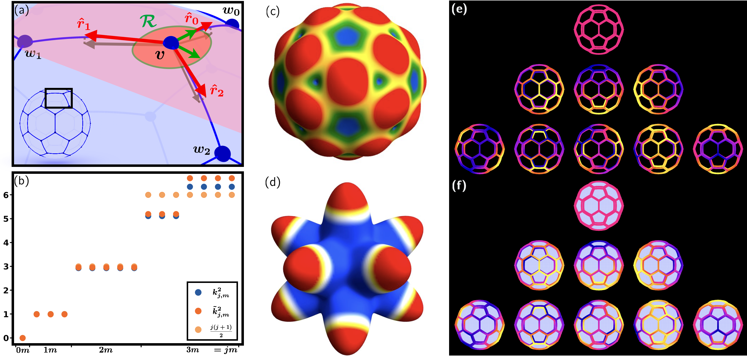
Figure 4: a) The truncated icosahedron (bottom left) is embedded within the 2-sphere $S^{2}$. The edge tensor $R$ acts on the tangent space of $S^{2}$, with the principle eigenvector (green) along the edge (red) opposite the local pentagonal face. (b) The graph eigenvalues $k_{j,m}^{2}$ track the PDE eigenvalues $\tilde{k}_{j,m}$, including splittings and multiplicities, even when discreteness effects are far from negligible. (c) Surface showing the largest local eigenvalue of $R$, i.e., $1+\varepsilon\sqrt{\text{tr}\!\left({S^{2}}\right)/2}$. (d) Surface illustrating the $\mu_{6}$ vertex density truncation. (e) & (f) graph eigenmodes & graph-restricted PDE eigenmodes respectively with rows$\,=\!j$, columns$\,=\!m$ for $|m|\leq{j}\leq 2$.

Conclusions

We present a PDE approach to metric graphs for modelling complex networks of nodes connected via continuous edges. The model is not intended to represent metric graph dynamics exactly in all settings. Rather, we present the examples in this work to show the pragmatic alikeness of the continuum, sometimes with only moderately dense networks. The model presented here is similar to “constitutive equation” approaches in other topics, like Murray’s law or Darcy-Brinkman in porous media [90, 91, 92, 93, 94], and the Q-tensor in liquid-crystal or polymer fluidics modelling [81, 95, 96, 97, 98]. The idea for future applications is to start from the PDE standpoint and construct empirically plausible edge tensors $R$ and vertex densities $\mu$. We are particularly intrigued by the possibility of using different $R$, $\mu$ parameters to model different brain regions in complex neuron tissue. Other future work should consider nonlinear effects in dense metric graph material, where the macroscopic parameters could respond dynamically to underlying changes in graph morphology.

Materials and methods

Code for the numerical simulations can be found at https://github.com/sidneyholden1/laplace_operator_metric_graph.

Acknowledgements

Both authors thank Robby Marangell for conversations about the remarkable properties of quantum graphs. We also thank Alexander Morozov for helpful comments on the manuscript.

References

- Berkolaiko and Kuchment [2013] G. Berkolaiko and P. Kuchment, Introduction to quantum graphs, Mathematical Surveys and Monographs, Vol. 186 (American Mathematical Soc., 2013).
- Pauling [1936] L. Pauling, The Journal of chemical physics 4, 673 (1936).
- Rawlinson [2018] J. I. Rawlinson, Nuclear physics. A 975, 122 (2018).
- Rawlinson [2019] J. I. Rawlinson, The Journal of chemical physics 151, 164303 (2019).
- Halcrow and Rawlinson [2020] C. J. Halcrow and J. I. Rawlinson, Physical review. C 102 (2020).
- Simkö et al. [2023] I. Simkö, C. Fäbri, and A. G. Csäszär, Journal of chemical theory and computation 19, 42 (2023).
- Rawlinson et al. [2021] J. I. Rawlinson, C. Fäbri, and A. G. Csäszär, Chemical communications (Cambridge, England) 57, 4827 (2021).
- Fábri et al. [2017] C. Fábri, M. Quack, and A. G. Császár, The Journal of Chemical Physics 147, 134101 (2017).
- Chiu et al. [2022] C. S. Chiu, A. N. Carroll, N. Regnault, and A. A. Houck, Physical Review Research 4, 023063 (2022).
- Hagel et al. [2021] J. Hagel, S. Brem, C. Linderälv, P. Erhart, and E. Malic, Physical Review Research 3, 043217 (2021).
- Cao et al. [2018a] Y. Cao, V. Fatemi, S. Fang, K. Watanabe, T. Taniguchi, E. Kaxiras, and P. Jarillo-Herrero, Nature 556, 43 (2018a).
- Cao et al. [2018b] Y. Cao, V. Fatemi, A. Demir, S. Fang, S. L. Tomarken, J. Y. Luo, J. D. Sanchez-Yamagishi, K. Watanabe, T. Taniguchi, E. Kaxiras, et al., Nature 556, 80 (2018b).
- Amovilli et al. [2004] C. Amovilli, F. E. Leys, and N. H. March, Journal of mathematical chemistry 36, 93 (2004).
- Leys et al. [2004] F. E. Leys, C. Amovilli, and N. H. March, Journal of chemical information and computer sciences 44, 122 (2004).
- de Oliveira and Rocha [2022] C. R. de Oliveira and V. L. Rocha, Reports on Mathematical Physics 89, 231 (2022).
- Fisher et al. [2021] L. Fisher, W. Li, and S. P. Shipman, Communications in Mathematical Physics 385, 1499 (2021).
- Lawrie et al. [2022] T. Lawrie, G. Tanner, and D. Chronopoulos, Scientific Reports 12, 1 (2022).
- Doron et al. [1990] E. Doron, U. Smilansky, and A. Frenkel, Physical review letters 65, 3072 (1990).
- Hul et al. [2004] O. Hul, S. Bauch, P. Pakoński, N. Savytskyy, K. Życzkowski, and L. Sirko, Physical review. E, Statistical physics, plasmas, fluids, and related interdisciplinary topics 69, 7 (2004).
- Ławniczak et al. [2019] M. Ławniczak, J. Lipovský, and L. Sirko, Physical review letters 122, 140503 (2019).
- Yunko et al. [2020] V. Yunko, M. Białous, and L. Sirko, Physical review. E 102, 012210 (2020).
- Lu et al. [2020] J. Lu, J. Che, X. Zhang, and B. Dietz, Physical review. E 102, 022309 (2020).
- Arnold et al. [2016] D. N. Arnold, G. David, D. Jerison, S. Mayboroda, and M. Filoche, Physical Review Letters 116, 056602 (2016).
- Filoche et al. [2017] M. Filoche, M. Piccardo, Y.-R. Wu, C.-K. Li, C. Weisbuch, and S. Mayboroda, Physical Review B 95, 144204 (2017).
- Piccardo et al. [2017] M. Piccardo, C.-K. Li, Y.-R. Wu, J. S. Speck, B. Bonef, R. M. Farrell, M. Filoche, L. Martinelli, J. Peretti, and C. Weisbuch, Physical Review B 95, 144205 (2017).
- Li et al. [2017] C.-K. Li, M. Piccardo, L.-S. Lu, S. Mayboroda, L. Martinelli, J. Peretti, J. S. Speck, C. Weisbuch, M. Filoche, and Y.-R. Wu, Physical Review B 95, 144206 (2017).
- Gebhard et al. [2022] F. Gebhard, A. V. Nenashev, K. Meerholz, and S. D. Baranovskii, “Quantum states in disordered media. i. low-pass filter approach,” (2022), arXiv:2212.00633 .
- Harrell II and Maltsev [2019] E. M. Harrell II and A. V. Maltsev, Transactions of the American Mathematical Society 373, 1701 (2019).
- Schanz and Smilansky [2000] H. Schanz and U. Smilansky, Physical Review Letters 84, 1427 (2000).
- Hislop and Post [2009] P. D. Hislop and O. Post, Waves in Random and Complex Media 19, 216 (2009).
- Klopp and Pankrashkin [2009] F. Klopp and K. Pankrashkin, Letters in Mathematical Physics 87, 99 (2009).
- Sabri [2014] M. Sabri, Reviews in Mathematical Physics 26, 1350020 (2014).
- Damanik et al. [2020] D. Damanik, J. Fillman, and S. Sukhtaiev, Mathematische Annalen 376, 1337 (2020).
- Gaio et al. [2019] M. Gaio, D. Saxena, J. Bertolotti, D. Pisignano, A. Camposeo, and R. Sapienza, Nature Communications 10 (2019), 10.1038/s41467-018-08132-7.
- Brio et al. [2022] M. Brio, J. G. Caputo, and H. Kravitz, “Localized eigenvectors on metric graphs,” (2022), arXiv:2203.09635 .
- Suja et al. [2017] M. Suja, S. B. Bashar, B. Debnath, L. Su, W. Shi, R. Lake, and J. Liu, Scientific Reports 7 (2017), 10.1038/s41598-017-02791-0.
- Jeong et al. [2022] B. Jeong, R. Akter, J. Oh, D.-G. Lee, C.-G. Ahn, J.-S. Choi, M. Rahman, et al., Scientific Reports 12, 1 (2022).
- Kulce et al. [2021] O. Kulce, D. Mengu, Y. Rivenson, and A. Ozcan, Light: Science & Applications 10 (2021), 10.1038/s41377-020-00439-9.
- Bassett and Sporns [2017] D. S. Bassett and O. Sporns, Nature neuroscience 20, 353 (2017).
- Menzel et al. [2020] M. Menzel, M. Axer, H. De Raedt, I. Costantini, L. Silvestri, F. S. Pavone, K. Amunts, and K. Michielsen, Physical Review X 10, 021002 (2020).
- Markram [2006] H. Markram, Nature reviews. Neuroscience 7, 153 (2006).
- Okano et al. [2016] H. Okano, E. Sasaki, T. Yamamori, A. Iriki, T. Shimogori, Y. Yamaguchi, K. Kasai, and A. Miyawaki, Neuron (Cambridge, Mass.) 92, 582 (2016).
- Amunts et al. [2016] K. Amunts, C. Ebell, J. Muller, M. Telefont, A. Knoll, and T. Lippert, Neuron (Cambridge, Mass.) 92, 574 (2016).
- Elam et al. [2021] J. S. Elam, M. F. Glasser, M. P. Harms, S. N. Sotiropoulos, J. L. Andersson, G. C. Burgess, S. W. Curtiss, R. Oostenveld, L. J. Larson-Prior, J.-M. Schoffelen, et al., NeuroImage 244, 118543 (2021).
- Montbrió et al. [2015] E. Montbrió, D. Pazó, and A. Roxin, Physical Review X 5, 021028 (2015).
- Martinello et al. [2017] M. Martinello, J. Hidalgo, A. Maritan, S. Di Santo, D. Plenz, and M. A. Muñoz, Physical Review X 7, 041071 (2017).
- Kadmon and Sompolinsky [2015] J. Kadmon and H. Sompolinsky, Physical Review X 5, 041030 (2015).
- Esfandiary et al. [2020] S. Esfandiary, A. Safari, J. Renner, P. Moretti, and M. A. Muñoz, Physical Review Research 2, 043291 (2020).
- Tang et al. [2011] G. Tang, K. Xu, and L. Jiang, Physical Review E 84 (2011), 10.1103/physreve.84.046207.
- Spiegler and Jirsa [2013] A. Spiegler and V. Jirsa, NeuroImage 83, 704 (2013).
- Steinmetz and Prota [2018] M. O. Steinmetz and A. E. Prota, Trends in Cell Biology 28, 776 (2018).
- Fürthauer et al. [2019] S. Fürthauer, B. Lemma, P. J. Foster, S. C. Ems-McClung, C.-H. Yu, C. E. Walczak, Z. Dogic, D. J. Needleman, and M. J. Shelley, Nature Physics 15, 1295 (2019).
- Stein et al. [2021] D. B. Stein, G. D. Canio, E. Lauga, M. J. Shelley, and R. E. Goldstein, Physical Review Letters 126 (2021), 10.1103/physrevlett.126.028103.
- Yan et al. [2022] W. Yan, S. Ansari, A. Lamson, M. A. Glaser, R. Blackwell, M. D. Betterton, and M. Shelley, eLife 11 (2022), 10.7554/elife.74160.
- Foster et al. [2019] P. J. Foster, S. Fürthauer, M. J. Shelley, and D. J. Needleman, Current Opinion in Cell Biology 56, 109 (2019).
- Exner et al. [2008] P. Exner, J. P. Keating, P. Kuchment, A. Teplyaev, and T. Sunada, Analysis on Graphs and Its Applications: Isaac Newton Institute for Mathematical Sciences, Cambridge, UK, January 8-June 29, 2007, Vol. 77 (American Mathematical Soc., 2008).
- Berkolaiko et al. [2006] G. Berkolaiko et al., Quantum Graphs and Their Applications: Proceedings of an AMS-IMS-SIAM Joint Summer Research Conference on Quantum Graphs and Their Applications, June 19-23, 2005, Snowbird, Utah, Vol. 415 (American Mathematical Soc., 2006).
- Mugnolo [2015] D. Mugnolo, Mathematical Technology of Networks: Bielefeld, December 2013, Vol. 128 (Springer, 2015).
- Post [2012] O. Post, Spectral analysis on graph-like spaces, Vol. 2039 (Springer Science & Business Media, 2012).
- Exner and Kovařík [2015] P. Exner and H. Kovařík, Quantum waveguides (Springer, 2015).
- Dáger and Zuazua [2006] R. Dáger and E. Zuazua, Wave propagation, observation and control in 1-d flexible multi-structures, Vol. 50 (Springer Science & Business Media, 2006).
- Mugnolo [2014] D. Mugnolo, Semigroup methods for evolution equations on networks, Vol. 20 (Springer, 2014).
- Chapman et al. [2015] S. J. Chapman, D. P. Hewett, and L. N. Trefethen, SIAM Review 57, 398 (2015).
- Lieb et al. [2016] A. M. Lieb, C. H. Rycroft, and J. Wilkening, SIAM Journal on Applied Mathematics 76, 1492 (2016).
- Cattaneo [1997] C. Cattaneo, Monatshefte für Mathematik 124, 215 (1997).
- Pankrashkin [2006] K. Pankrashkin, Letters in Mathematical Physics 77, 139 (2006).
- Exner et al. [2018] P. Exner, A. Kostenko, M. Malamud, and H. Neidhardt, in Annales Henri Poincaré, Vol. 19 (Springer, 2018) pp. 3457–3510.
- Carlson [2008] R. Carlson, Analysis on graphs and its applications 77, 355 (2008).
- Carlson [2012] R. Carlson, Networks and Heterogeneous Media 7, 483 (2012).
- Exner et al. [2006a] P. Exner, P. Hejčík, and P. Šeba, Reports on Mathematical Physics 57, 445 (2006a).
- Nakamura and Tadano [2021a] S. Nakamura and Y. Tadano, Journal of Spectral Theory 11, 355 (2021a).
- Exner et al. [2022a] P. Exner, S. Nakamura, and Y. Tadano, Letters in Mathematical Physics 112 (2022a), 10.1007/s11005-022-01576-5.
- Carlson [2006] R. Carlson, Contemporary Mathematics 415, 65 (2006).
- Maury et al. [2009] B. Maury, D. Salort, and C. Vannier, Networks & Heterogeneous Media 4, 469 (2009).
- and [2014] R. C. and, Networks and Heterogeneous Media 9, 477 (2014).
- Pokornyi and Borovskikh [2004] Y. V. Pokornyi and A. Borovskikh, Journal of Mathematical Sciences 119, 691 (2004).
- Tzella and Vanneste [2016] A. Tzella and J. Vanneste, Physical Review Letters 117 (2016), 10.1103/physrevlett.117.114501.
- van der Hoorn et al. [2021] P. van der Hoorn, W. J. Cunningham, G. Lippner, C. Trugenberger, and D. Krioukov, Physical Review Research 3, 013211 (2021).
- sup [2023] Supplemental_Material (2023).
- Evans and Garzepy [2018] L. C. Evans and R. F. Garzepy, Measure theory and fine properties of functions (Routledge, 2018).
- Gennes [1971] P. G. D. Gennes, Molecular Crystals and Liquid Crystals 12, 193 (1971).
- Exner et al. [2006b] P. Exner, P. Hejčík, and P. Šeba, Reports on Mathematical Physics 57, 445 (2006b).
- Pankrashkin [2012] K. Pankrashkin, Journal of Mathematical Analysis and Applications 396, 640 (2012).
- Nakamura and Tadano [2021b] S. Nakamura and Y. Tadano, Journal of Spectral Theory 11, 355 (2021b).
- Exner et al. [2022b] P. Exner, S. Nakamura, and Y. Tadano, Letters in Mathematical Physics 112 (2022b), 10.1007/s11005-022-01576-5.
- Berry [1984] M. V. Berry, Proceedings of the Royal Society of London. A. Mathematical and Physical Sciences 392, 45 (1984).
- Burns et al. [2020] K. J. Burns, G. M. Vasil, J. S. Oishi, D. Lecoanet, and B. P. Brown, Physical Review Research 2, 023068 (2020).
- Vasil et al. [2019] G. M. Vasil, D. Lecoanet, K. J. Burns, J. S. Oishi, and B. P. Brown, Journal of Computational Physics: X 3, 100013 (2019).
- Lecoanet et al. [2019] D. Lecoanet, G. M. Vasil, K. J. Burns, B. P. Brown, and J. S. Oishi, Journal of Computational Physics: X 3, 100012 (2019).
- Murray [1926] C. D. Murray, Proceedings of the National Academy of Sciences 12, 207 (1926).
- Brinkman [1949] H. C. Brinkman, Flow, Turbulence and Combustion 1 (1949), 10.1007/bf02120313.
- Weinbaum et al. [2003] S. Weinbaum, X. Zhang, Y. Han, H. Vink, and S. C. Cowin, Proceedings of the National Academy of Sciences 100, 7988 (2003).
- Holter et al. [2017] K. E. Holter, B. Kehlet, A. Devor, T. J. Sejnowski, A. M. Dale, S. W. Omholt, O. P. Ottersen, E. A. Nagelhus, K.-A. Mardal, and K. H. Pettersen, Proceedings of the National Academy of Sciences 114, 9894 (2017).
- Chen et al. [2022] M. Chen, X. Shen, Z. Chen, J. H. Y. Lo, Y. Liu, X. Xu, Y. Wu, and L. Xu, Proceedings of the National Academy of Sciences 119 (2022), 10.1073/pnas.2207630119.
- Schopohl and Sluckin [1987] N. Schopohl and T. J. Sluckin, Physical Review Letters 59, 2582 (1987).
- Wensink et al. [2012] H. H. Wensink, J. Dunkel, S. Heidenreich, K. Drescher, R. E. Goldstein, H. Löwen, and J. M. Yeomans, Proceedings of the National Academy of Sciences 109, 14308 (2012).
- Zhang et al. [2017] R. Zhang, N. Kumar, J. L. Ross, M. L. Gardel, and J. J. de Pablo, Proceedings of the National Academy of Sciences 115 (2017), 10.1073/pnas.1713832115.
- Mackay et al. [2020] F. Mackay, J. Toner, A. Morozov, and D. Marenduzzo, Physical Review Letters 124 (2020), 10.1103/physrevlett.124.187801.