Using massless fields for observing black hole features in the collapsed phase of Euclidean dynamical triangulations

Abstract

We report on an old computation of propagators of massless scalar fields on an ensemble of configurations in the 4D path integral of Euclidean dynamical triangulations in the collapsed (crumpled) phase. The resulting quantum average is used to calculate the scale factor of a rotational invariant metric in a 4-dimensional space. This new scale factor is non-zero at the origin, which we assume to be caused by the presence of the well-known singular structure in the collapsed phase. It depends on an overall integration constant. A transformation to a metric in (1+3)-dimensions reveals Euclidean black hole features at an instant in time, with a horizon separating interior and exterior parts. Effective Einstein equations in the presence of a ‘geometric condensate’ are assumed, and computed with the software OGRe. We find similarities with the energy density and pressure of gravastars, as well as with remnants, and investigate their dependence on the integration constant.

I Introduction

In the dynamical triangulation approach to Euclidean quantum gravity (EDT) the configurations of the regulated path integral form a lattice consisting of equilateral four-simplexes ‘glued’ together [1, 2, 3] (for reviewing texts see e.g. [4, 5, 6, 7]). A scenario for a continuum limit has been proposed [7] for a model with three parameters, two of which monitor the (bare) Newton and cosmological couplings, $G_{{\rm N}0}$ and $\Lambda_{0}$, the third controls a ‘measure term. This measure term is a local factor in the summation measure over configurations [8, 9] which can be written as a term in the action that depends logarithmically on the Regge curvature [5, 10] (initially a different one was introduced in [11], recently revisited in [12]).

A customary notation uses dimensionless parameters $\kappa_{2}\propto 1/G_{{\rm N}0}$ and $\kappa_{4}\leftrightarrow\Lambda_{0}$, and $\beta$ for the measure term. Numerical simulations have revealed two phases, a ‘collapsed phase’ (a.k.a. ‘crumpled phase’) at strong coupling and an ‘elongated phase’ at weak coupling, separated by a first-order transition line in the $\kappa_{2}$-$\beta$ phase diagram [13, 14, 6, 15, 10]. In the scenario of [7] the continuum limit is to be approached along the phase boundary on the collapsed side towards weaker couplings, i.e. larger $\kappa_{2}$.

Similar phases appear in the formulation using well-defined time slices called ‘causal dynamical triangulation (CDT) [16, 17, 18], and approaches to a possible UV fixed point along ‘lines of constant physics’ are described in [19, 20, 21].

A continuum limit towards a phase boundary from the strong coupling side is also proposed in a different formulation with variable lattice edge lengths [22, 23].

The original EDT formulation had no measure term, i.e. $\beta=0$ [1, 2]. Numerical simulations at $\beta=0$ revealed that the two phases have very distinct properties. The ‘elongated phase’ is dominated by baby universes with branched polymer characteristics [24]. In the collapsed phase a ‘singular structure’ appears consisting of two adjacent vertices that belong to a macroscopic number of four-simplexes (growing linearly with the lattice size) [25, 26, 27, 28, 29].

Visualizations of typical configurations at $\beta=0$ show fractal tree-like ‘branched-polymer’ structures in the elongated phase and a dense ‘blob’ with trees sticking out in the collapsed phase [6, 15, 7]. Branched polymers have been linked to conformal fields [30, 31] and one can imagine the blob as representing a naked singularity or a black hole, and the trees representing a boundary field theory, similar to AdS/CFT [32, 33, 34]. At negative $\beta$, upon increasing $-\beta$ and $\kappa_{2}$ the system enters a region called ‘crinkled’ [8, 9] in which the blob stratifies and includes larger distances [6, 10] with an accompanying smaller lattice spacing [7]. These features suggest studying quantal properties of black-holes by simulations in EDT.

At $\beta=0$ there will be lattice artefacts in the results but they may still inform us about quantum-gravitational physics. The great advantage of the numerical simulations is that they yield truly non-perturbative results which can qualitatively and even semi-quantitatively describe physics. We recall that lattice QCD at strong coupling (i.e. far from its continuum limit) gives a fair characterization of the low mass hadrons (as summarized for example in [35], section 7.4).

In [36, 37] gravitational binding energy between two massive scalars was computed in EDT in the quenched approximation (in perturbation theory this corresponds to leaving out closed particle loops). A non-zero binding energy $E_{\rm b}$ came out, with a dependence on the particle masses $m$ that was not understood. A recent study [38] suggested an explanation in terms of a blow-up effect in the bound state wave function causing finite-size squeezing of the system with a decreasing ratio $E_{\rm b}/m$ with increasing $m$, in a large mass region. The effect is proportional to $m\,G_{\rm N}$, with $G_{\rm N}$ a renormalized Newton coupling. In an elaborate analysis of the results in [36] the renormalized Planck length $\sqrt{G_{\rm N}}$ was estimated to be fairly large ($\approx 8$) in lattice units, near the phase transition on the collapsed side. The relevance of the black hole scale $m\,G_{\rm N}$ came as a surprise. (This explanation needs confirmation on larger lattices.)

A controlled computation of the binding energy appeared in [39]. This work used extrapolation to the continuum limit in the above mentioned scenario, scale-dependent dimensions allowing relatively small lattices and extrapolation to infinite volume, with the result $\sqrt{G_{\rm N}}=3.9\pm 0.7$ in lattice units. A similar value was subsequently found using a completely different method [40]. These computations employed a different ensemble of so-called degenerate triangulations [3]. (In [38] (and below) the analysis uses dimension 4 which requires avoiding short distances.)

In [41] effective curvature observables based on a ‘volume-distance correlator’ were computed which showed locally negative curvature in the collapsed phase and locally positive curvature in the elongated phase. This was refined further in [42] into effective metrics describing an average geometry that is approximately locally hyperbolic and spherical, respectively.

The present work focuses on the collapsed phase away from the phase transition. We present results for the propagators of massless scalar-fields obtained from simulations in 1996 by B.V. de Bakker in collaboration with the present author. The negative curvature in the collapsed phase found earlier raised the question whether this would be confirmed by an exponential decay of massless propagators at large distances, as in hyperbolic space in the continuum. Evidence for such decay was indeed found and briefly mentioned in [43], but for logistic reasons the write-up got stuck at the stage of ‘a draft of a draft’ [44]. Part of these results could be recovered recently. They are analyzed here further and used to derive, in a fundamentally different way, metrics for average geometries as observed through the propagators.

The propagator reacts to the quantum geometries in a way that fundamentally differs from the volume-distance observable. A clue to an explanation may be found in the plot in figure 2.7 of [45], which shows that a massless scalar field propagator on a configuration deep in the elongated phase becomes constant on the thin branches of its tree-like structure. It is reminiscent of the constancy of the electric potential in a Faraday cage. Our knowledge of distances is based primarily on electrodynamics involving the massless photon. In fact, on the Planck scale all fields in the Standard Model are practically massless. It is possible that observing quantum geometry with massless fields does not suffer from baby-universe fluctuations at the Planck scale.

The above mentioned volume-distance correlator is the average three-volume at a fixed distance from an arbitrary origin. With lattices of $S^{4}$ topology it leads naturally to isotropic average metrics of the form

$$ds^{2}=dr^{2}+a(r)^{2}\,d\Omega_{3}^{2}\,,$$ (1)

with $\mbox{d}\Omega_{3}$ the line-element on the unit three-sphere (an example is described in the appendix (A)). In the continuum, the scale factor $a(r)$ is closely related to the derivative of the four-volume $V(r)$ within distance $r$ from the origin:

$$V(r)=\int d\Omega_{3}\int_{0}^{r}d\bar{r}\,a(\bar{r})^{3}\,,\quad\partial_{r}V(r)=2\pi^{2}a(r)^{3}\,.$$ (2)

In the present work the important observable is the propagator $G(r)$ of a massless scalar field. In the continuum it has to satisfy the Laplace-Beltrami equation for the metric (1),

$$\left[\frac{d^{2}}{dr^{2}}+\frac{3}{a(r)}\frac{d}{dr}\,a(r)\right]G(r)=0\,,\quad r>0\,,$$ (3)

with appropriate boundary conditions.

Section II is a literal rendition of section 3 in the draft [44]. In it, $G(r)$ was presented for the hyperbolic metric

$$a(r)=r_{0}\sinh(r/r_{0})\,,$$ (4)

and its asymptotic behavior determined as $G(r)\propto\exp(-3r/r_{0})$. Its lattice version was numerically computed in the collapsed phase and found to be fitted well by the exponential form $G(r)\propto\exp(-mr)+\mbox{const.}$, where the constant represents a zero mode of the lattice version of the Laplace-Beltrami operator in (3).

In section III we find the fitted $m$ to be much smaller than the ‘predicted’ $3/r_{0}$ from the curvature radii $r_{0}$ obtained with volume-distance correlators, although their ratio as a function of $\kappa_{2}$ is nearly constant. It is concluded that the continuum $G(r)$ based on (4) cannot fit the lattice $G(r)$.

We change tactics in section IV and use (3) as a first-order differential equation for a scale factor $a(r)$. The solution is $a(r)=c_{G}\,[\partial_{r}G(r)]^{-1/3}$, with $c_{G}$ an integration constant. Replacing the continuum $\partial_{r}G(r)$ by a fit to its lattice data gives a new scale factor for the average quantum geometry.

This new metric comes out very different from (4). A major characteristic is that a function linear in $r^{2}$ approximates the data reasonably well at intermediate distances away from the origin, although the data deserves more elaborate fit functions. Their extrapolation to the origin should not suffer greatly from lattice artefacts or running dimensions and we assume this extrapolation to have physical significance.

The newly obtained scale factor $a(r)$ determines how the three-volume described by the metric grows with the distance from the origin, which depends on the integration constant $c_{G}$. Seeking to fix $c_{G}$ by comparison with the lattice $V(r)$ is a possible but not so well-defined endeavour (carried out at the end of appendix A) since we do not know the volume in polymer trees which the propagator is supposed to roughly ‘ignore’. Other possibilities are also considered in the following.

Section V follows up on the idea that the collapsed state may have properties showing the presence of a black hole, allowing also for a quantum mechanical ‘vacuum condensate’ [46, 47, 48, 49, 50, 51]. A transformation is made to spherical coördinates with line element

$$ds^{2}=g_{\tau\tau}(r,\tau)d\tau^{2}+2g_{r\tau}(r,\tau)dr\,d\tau+g_{rr}(r,\tau)dr^{2}+r^{2}\,d\Omega_{2}^{2}.$$ (5)

Here $d\Omega_{2}$ is the line element on $S^{2}$ with unit radius, $\tau$ is a Euclidean time variable and $r$ a radial coördinate in three dimensions – it differs from the $r$ in 4D above eq. (5). A companion article will present a study of such transformations which aims at forms in which the cross-term $g_{r\tau}$ vanishes and $g_{\tau\tau}=1/g_{rr}$. The transformation presented in section V incorporates important results of this study.

Assuming that the Einstein equations hold in the effective sense gives the form of the energy-momentum tensor of the condensate, $T^{\mu}_{\;\,\nu}$,

$$G^{\mu}_{\;\,\nu}=8\pi G_{\rm N}\,T^{\mu}_{\;\,\nu}\,,\quad G^{\mu}_{\;\,\nu}=R^{\mu}_{\;\,\nu}-\frac{1}{2}\,R\,\delta^{\mu}_{\;\,\nu}\,,$$ (6)

where $G_{\rm N}$ is a renormalized Newton constant. For the calculation the software OGRe [52] is very helpful. At $\tau=0$ a black hole appears with a Euclidean de Sitter (EdS) interior and properties similar to gravastars [50] and ‘regular black holes’ (for the latter see e.g. [53] and references therein).

The appendix (A) contains details of the EDT formulation and the volume-distance correlator. Units are used in which the dual lattice distance (the minimal distance between the centers of two 4-simplexes) $\tilde{\ell}=1$.

II Massless propagators

On a space with constant negative curvature, a massless propagator shows exponential fall off with the distance and can thus be viewed as having a mass.

Rewriting the equation for the massless propagator $\square\,G(x^{\mu})=0$ using spherical symmetry and a space of constant negative curvature with curvature radius $r_{0}$ we get

$$\left(\frac{d}{dr}+\frac{3\coth r/r_{0}}{r_{0}}\right)\frac{d}{dr}G(r)=0\,.$$ (7)

This can be exactly solved and using the boundary conditions

$$G(r) \to 0\,,\qquad\;r\to\infty\,,$$ (8)

$$G(r) \to \frac{1}{4\pi r^{2}}\,,\quad r\to 0\,,$$ (9)

and the solution is

$$G(r) = \frac{1}{4\pi r_{0}^{2}}\left\{2\frac{\exp(r/r_{0})+\exp(-r/r_{0})}{\left(\exp(r/r_{0})-\exp(-r/r_{0})\right)^{2}}\right.$$ (11)

$$\left.-\ln\frac{1+\exp(-r/r_{0})}{1-\exp(-r/r_{0})}\right\}.$$

Expanding this around $r\to\infty$ in $\exp(-r/r_{0})$ results in

$$G(r)=\frac{2}{4\pi r_{0}^{2}}\sum_{n=0}^{\infty}\frac{n(n+1)}{2n+1}\exp(-(2n+1)r/r_{0})\,.$$ (12)

We see that for large $r$ the massless propagator behaves as

$$G(r)\propto\exp(-3r/r_{0}),\quad r\to\infty\,.$$ (13)

If we define the mass $m$ from the long distance behaviour of the propagator using $G(r)\propto\exp(-mr)$, then this mass and the curvature radius are related by $mr_{0}=3$.

Figure 1: Averaged massless lattice propagators $G(r)$ for some values of $\kappa_{2}$ at $N_{4}=32000$.

On the lattice, we solved the Laplace equation $\square\,G(x^{\mu})=0$ using the algebraic multigrid routine AMG1R5. Figure 1 shows the results for the smallest volume $N_{4}=32000$. Note that we can add an arbitrary constant to $G(r)$. This constant is determined by the details of the computer code and has no physical meaning. This also means that the individual values of the data points have no meaning and therefore we have left out the error bars. This is not an obstacle to calculating the masses and their errors.

We fitted this data to $a\exp(-mr)+c$ in the range $6\leq r\leq 20$. The fits are also shown in figure 1.

Figure 2: Measured effective masses of propagators as a function of $\kappa_{2}$ for two values of $N_{4}$.

Figure 2 show the masses $m$ measured for various values of $\kappa_{2}$ at the two volumes that were used. The error bars were obtained by the jackknife method, leaving out one configuration each time. In this way the correlation between the data of two different origins on the same configuration does not artificially decrease the errors.

The configurations used for these measurements were recorded each $5000$ sweeps, where a sweep consists of $N_{4}$ accepted moves. For each configuration we used 200 different origins to calculate the propagator from. We could only measure these masses for a limited number of $\kappa_{2}$ values, because the calculation of the propagator takes much CPU time.

III Comparison of effective masses with curvature radii

The draft [54] contained two plots of simple local curvature-observables vs. $\kappa_{2}$ based on the volume-distance correlator, called $R_{V}$ and $R_{\rm eff}$. We shall not show these here since they were presented already in [42]; qualitatively, the falling of $m$ in figure 2 with increasing $\kappa_{2}$ resembles the diminishing of $\sqrt{|R_{V}|}$ and $\sqrt{|R_{\rm eff}|}$ in the collapsed phase. For a quantitative comparison with the asymptotic form (13) that predicts $mr_{0}/3=1$, we use $r_{0}$ results obtained in [42] for the volume $N_{4}=64$ k (cf. table (B.2)). Figure 3 shows a (so-called ‘continuum curvature’) $R_{\rm c}$ in both phases.

Numerical data files of the propagators and fitted parameters of $a\exp(-mr)+c$ are lost, unfortunately. However, we have retrieved values of $m$, and for $N_{4}=32$ k also the propagators, from the postscript files of figure 1 and 2.

Figure 4 shows the ratio $m/(3/r_{0})$ vs. $\kappa_{2}$ with the $r_{0}$ corresponding to figure 3 in which $N_{4}=64$ k. (With $N_{4}=32$ k only $\kappa_{2}=1.240$ and 1.245 volume-distance results are available.) The linearly varying ratio appears to confirm the negative-curvature interpretation of the average geometry in the collapsed phase. But the magnitude of the ratio is much smaller than 1. An immediate explanation is suggested by the fact that the effective-mass fits to the propagators involve larger distances (up to $r=20$) than the curvature fits to the volume-distance correlator which ended at $r=12$. But we shall conclude below that the discrepancy is more fundamental.

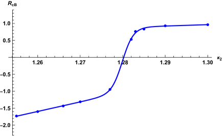
Figure 3: Curvature $R_{\rm c}$ vs. $\kappa_{2}$ obtained with the B-fit (dots) fitted by the function (8.6) in [42] ($N_{4}=64$ k, data from the Erratum).

Figure 4: The ratio $m/(3/r_{0})$ vs. $\kappa_{2}$ in the collapsed phase with $r_{0}$ values from the fit in figure 3 ($N_{4}=64$ k). The line is a linear fit by $10-7.7\,\kappa_{2}$.

Refitting the retrieved propagator data with the fit function $a\exp(-mr)+c$ in the domain $6\leq r\leq 24$, the fitted parameters came out as ($N_{4}=32$ k):

$$\begin{array}[]{cccccccccc}\kappa_{2}&c&a&m&r_{0m}\equiv 3/m&\\ 1.240&-0.0726&1.48&0.098&30.7\\ 1.245&-0.0816&1.62&0.081&37.2\\ 1.250&-0.148&2.04&0.056&53.5\\ 1.252&-0.167&2.14&0.051&58.9\end{array}$$ (14)

The effective curvature radii $r_{0m}$ are remarkably large. Our refitted $m$ are 20-30 % smaller than those in figure 2 (the original fit domain $6\leq r\leq 20$ in section II leads to even slightly smaller values and spoil the good looking fits in figure 5 for $r>20$). The re-fits are of the least-squares type whereas the error bars in figure 2 represent jack-knife errors, which tend to underestimate errors. Overlaying a print of the plot in figure 1 by a same size print for the propagators obtained with refitted parameters gives a perfect match visually. We ascribe the difference to small mis-representations by the postscript files and correlations in the fitted $a$, $m$ and $c$. It does not affect the exploring nature of this work.

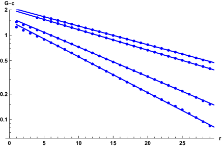
Figure 5: Propagators fitted by $c+a\exp(-mr)$ in the domain $6\leq r\leq 24$. Data and fit-function are both subtracted by $c$; top to bottom $\kappa_{2}=1.252$, 1.250, 1.245, 1.240; $N_{4}=32$k.

Figure 5 shows the obtained propagators shifted by $-c$ on a logarithmic scale. Exponential behavior is a fairly good approximation as can be seen quantitatively in figure 6 which shows the ratio (data-$c$)/($a\exp(-mr))$ for $\kappa_{2}=1.240$. In this case the deviations from 1 are at the percent level in the fit domain; for the other $\kappa_{2}$ such deviations are smaller by an order of magnitude. The local minimum near $r=18$ occurs where the volume-distance correlator has its maximum (cf. figure 14 in appendix A).

Remarkably, this maximum hardly affects the nearly exponential behavior of the shifted propagators. Surprising is also the fact that this behavior occurs all the way down to about $r=6$. It implies that using the exact form (11) of $G(r)$ in a fit function of the form $c+a\,G(r)$ cannot fit the data. (This becomes immediately clear when trying such fits. One also notes that $G(r)$ in (11) approaches the leading term in its asymptotic expansion to 1% accuracy only for $r/r_{0}>2.59$; for $\kappa_{2}=1.240$ this means $r>80$ !.)

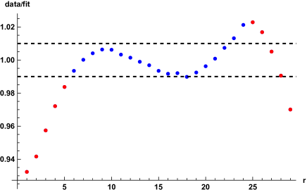
Figure 6: Subtracted propagator $G(r)-c$ divided by subtracted fit-function $a\exp(-mr)$, for $\kappa_{2}=1.240$. The blue(red) points are inside(outside) the fit domain.

IV Metric scale factor from measured propagator

Having obtained $G(r)$ from the numerical simulation we now use the relation (3) to define an average metric scale factor as ‘seen’ by the propagator, by treating (3) as a differential equation for $a(r)$:

$$3\,\partial_{r}\ln[a(r)]=-\partial_{r}\ln\left[-\partial_{r}G(r)\right]\,.$$ (15)

The solution for $a(r)$ has a multiplicative integration constant,

$$a(r)\propto\left[-\frac{1}{\partial_{r}G(r)}\right]^{1/3}\,.$$ (16)

On the lattice we implement the discrete derivative as

$$G^{\prime}(r+1/2)=G(r+1)-G(r)\,,$$ (17)

and define a lattice version of the scale factor by

$$a_{G}(r)=\left[-\frac{1}{G^{\prime}(r)}\right]^{1/3}\,.$$ (18)

The scale factor to represent the average geometry in the continuum contains the multiplicative integration constant $c_{G}$,

$$a(r)=c_{G}\,a_{G}(r)\,.$$ (19)

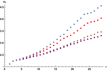
Figure 7: Lattice $a_{G}(r)$, top to bottom $\kappa_{2}=1.240$, 1.245, 1.250, 1.252; $N_{4}=32$k.

Results are available for $\kappa_{2}=1.240$, 1.245, 1.250 and 1.252 at $N_{4}=32$ k. Figure 7 shows $a_{G}(r)$ for these $\kappa_{2}$. In this study of the collapsed phase it is important that $\kappa_{2}$ is sufficiently far from the phase transition. Judging from the broad susceptibility peak in figure 14 of [42], this holds for $\kappa_{2}=1.240$, and to a lesser extent for $\kappa_{2}=1.245$ which appears located at the edge of the peak. But the two larger $\kappa_{2}$ have penetrated the susceptibility peak and indeed, their points plotted in figure 7 appear separated from the two lower $\kappa_{2}$. In the following we concentrate primarily on case $\kappa_{2}=1.240$.

The first three data points at $r=1.5$, 2.5 and 3.5 where all $\kappa_{2}$ data merge visually are presumably strongly subjected to lattice artefacts; discarding these, a mental extrapolation to $r=0$ suggests a non-zero $a_{G}(0)\approx 2.3$.

The pennant-like feature of the last five data points ($r\geq 24.5$) is present in both $\kappa_{2}=1.240$ and 1.245 which suggests that it is not due to statistical fluctuations. It may indicate a drop in the contributing volume near $r=25$ and also a change in the character of contributing geometries.

At large distances we expect branched polymers to become important in a broad transition region starting at $r=25$ (cf. appendix A). As mentioned in the Introduction, figure 2.7 in [45] indicates that $G(r)$ flattens and becomes nearly constant on minimal neck polymers. This will cause a rapid increase of $a_{G}(r)$.

Of particular interest to our analysis turns out to be the region near the origin $r=0$. To avoid strong lattice artefacts and variable dimension effects we shall reach this region by extrapolation from $r\geq 5.5$ towards zero. A good choice of fit function and fit domain appears to be given by

$$f_{\rm rat}(r)=\frac{p_{0}+p_{1}\,r^{2}}{1+q\,r^{2}}\,,\quad 5.5\leq r\leq 23.5\,.$$ (20)

It does significantly better than a mere quadratic fit $p_{0}+p_{1}r^{2}$ in the region $r\geq 19.5$, and even in $r\leq 7.5$. The exponential fit made already for the propagator

$$f_{\rm e}(r) = [-\partial_{r}(c+a\exp(-mr)]^{-1/3}$$ (21)

$$= (3a/r_{0m})^{-1/3}\,\exp(r/r_{0m})\,,$$

gives a good description of the data in $7.5\leq r\leq 18.5$ with the parameters of (14). For analytic treatment the simple form

$$f_{\rm ch}(r)=c_{\rm ch}\cosh(r/r_{0})$$ (22)

is useful with the same fit domain as in (20). Qualitatively $f_{\rm ch}(r)$ is similar to $f_{\rm rat}(r)$ in the fit domain and it approaches asymptotically a Euclidean Anti-de Sitter (EAdS) scale factor with length scale $r_{0}$. However, here $r_{0}$ monitors primarily quadratic behavior at small and intermediate distances. The fitted parameters for the lowest two $\kappa_{2}$ for $f_{\rm rat}(r)$ are given by

$$\begin{array}[]{cccccccccc}\kappa_{2}&p_{0}&p_{1}&q_{1}&p_{1}/p_{0}-q_{1}&\\ 1.240&2.24&0.00447&0.000219&0.0018\\ 1.245&2.23&0.00497&0.000616&0.0016\end{array}\,.$$ (23)

The combination $p_{1}/p_{0}-q_{1}$ is the coefficient of $r^{2}$ in the expansion $f(r)=f(0)+\frac{1}{2}\,f^{\prime\prime}(0)r^{2}+\cdots$. Fits are shown in figure 8 for $\kappa_{2}=1.240$. For the cosh-model we only mention $c_{\rm ch}=2.32$, $r_{0}=22$ for $\kappa_{2}=1.240$, since this fit function will not be used further in this article.

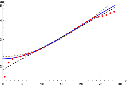
Figure 8: Log-plot of $a_{G}(r)$ data (dots) and fit functions $f_{\rm rat}$ (blue curve), $f_{\rm ch}$ (dashed brown curve), and $f_{\rm e}(r)$ (dashed black straight line); $N_{4}=32$ k, $\kappa_{2}=1.240$.

A fit function with EAdS asymptotics in which the scale $r_{0}$ is decoupled from the small and intermediate region is

$$f_{\rm ratch}(r)=f_{\rm rat}(r)f_{\rm ch}(r)\,,\quad c_{\rm ch}=1\,,\quad r_{0}=r_{0{\rm m}}\,.$$ (24)

With the choice $r_{0}=r_{0{\rm m}}$, refitting the parameters of the factor $f_{\rm rat}(r)$ gives an equally good fit as $f_{\rm rat}(r)$ on its own. However, with the moderate-size lattices used here, evidence for EAdS asymptotic behavior is not strong.

The scalar curvature can be calculated from

$$R(r)=6\left[-\frac{a^{\prime\prime}(r)}{a(r)}-\frac{a^{\prime}(r)^{2}}{a(r)^{2}}+\frac{1}{a(r)^{2}}\right]\,.$$ (25)

With $a(r)=c_{G}\,f_{\rm rat}(r)$ this becomes a rational function in which numerator and denominator are polynomials of the 4-th degree in $r^{2}$. At the origin it simplifies to

$$R_{\rm rat}(0)=\frac{6}{c_{G}^{2}\,p_{0}^{2}}-\frac{12\,p_{1}}{p_{0}}+12\,q_{1}\,.$$ (26)

The metric scale factor $a(r)=c_{G}\,a_{G}(r)$ is completed by specifying the integration constant $c_{G}$. We mention three choices:

• Equate $V(r)=\int d\Omega_{3}\,\int_{0}^{r}d\bar{r}\,a(\bar{r})^{3}$ with the four-volume of the simplexes in a ball within distance $r$ from the origin. Fits discussed below give $c_{G}\approx 1.5$.

• Impose $R(0)=0$, which leads to negative curvature away from the origin:

  $$c_{G}=\frac{1}{\sqrt{2}\,p_{0}\sqrt{p_{1}/p_{0}-q_{1}}}\equiv c_{G0}\,.$$ (27)

  The fit result is $c_{G0}=7.49$.

• Equate the surface gravity of the ‘instantaneous black hole’ encountered in the next section with the Schwarzschild case, eq. (42), then $c_{G{\rm S}}=5.3$.

The first case is not straight-forward since $G(r)$ is assumed to practically ‘ignore’ the volume of branched-polymer ‘hair’ of the blobs mentioned in the Introduction. An implementation with the proposition that the hair only contributes to the region $r>r_{\rm blob}$ and the volume in the blobs is equal to $V(r_{\rm blob})$ leads to $c_{G}\simeq 1.5$ (cf. end of appendix A). The resulting curvature $R(r)$ is relatively large (by an order of magnitude compared to the other cases) and positive. This stems from the curvature term $6/a(r)^{2}$ in (25) coming from the $S^{3}$ sphere with radius $a(r)\propto c_{G}$ and a relatively small $c_{G}$.

The second case is more in line with the original motivation of a negative-curvature collapsed phase. The curvatures for the second and third cases are shown in figure 9.

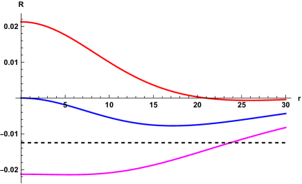
Figure 9: Scalar curvatures for various $c_{G}$. Upper curve (red): $c_{G}=c_{G{\rm S}}=5.3$; middle curve (blue): $c_{G}=c_{G0}=7.5$; lower curve (magenta): $c_{G}=\infty$. The dashed line (black) is $-12/r_{0{\rm m}}^{2}$ with $r_{0{\rm m}}=30.7$ from (14).

V Black hole features

Black hole and similar geometries with rotational symmetry are usually studied in spherical coordinates. In imaginary time $\tau$, line elements have the form

$$ds^{2}=g_{\tau\tau}(r,\tau)\,d\tau^{2}+2\,g_{rr}(r,\tau)\,dr^{2}+r^{2}\,d\Omega_{2}^{2}\,,$$ (28)

in which $r$ is a radial coordinate in three dimensions. The radial coordinate in four dimensions used in the previous sections was also called $r$ and to avoid confusion we shall denote it in this section by $\eta$,

$$ds^{2} = d\eta^{2}+a(\eta)^{2}\,d\Omega_{3}^{2}$$ (29)

$$= d\eta^{2}+a(\eta)^{2}\,d\psi^{2}+a(\eta)^{2}\,\sin(\psi)^{2}\,d\Omega_{2}^{2}\,,$$

($0<\psi<\pi$). For the rational function fit

$$a(\eta)=c_{G}\,f_{\rm rat}(\eta)=c_{G}(p_{0}+p_{1}\,\eta^{2})/(1+q_{1}\,\eta^{2})\,.$$ (30)

Transformations of variables of the form

$$r = a(\eta)\,\sin\psi\,,\quad y=a(\eta)\,\cos\psi\,,\quad y=y(r,\tau)\,,$$ (31)

$$\eta = a_{\rm inv}(\sqrt{r^{2}+y^{2}})\;,\psi=\arctan(y,r)\,,$$ (32)

where $a_{\rm inv}(a)$ is the inverse function of $a(\eta)$, turn (29) into (28) and conversely. The maximal value of $r$ is obtained when $\psi=\pi/2$ and $a(\eta)$ is maximal; we denote it by $r_{\rm b}$, $r_{\rm b}=a_{\rm max}\approx 4.5\,c_{G}$ (cf. figure 8), and denote $a(0)=h$. A study of various functions $f(r,\tau)$ is delegated to a companion article. Here we just summarize for the rational function fit the effect of choosing

$$y(r,\tau) = \sqrt{F(r)}\,\tau\,,\qquad\;h<r<r_{\rm b}\,,$$ (33)

$$= \sqrt{h^{2}-r^{2}}\,\,(1+c_{\tau}\,\tau^{2})\,,\quad 0<r<h\,,$$ (34)

$$F(r) = \frac{4(r-h)(c_{G}\,p_{1}-q_{1}r)^{3}}{h^{2}(p_{1}/p_{0}-q_{1})^{2}}\,,$$ (35)

$$c_{\tau} = 2(p_{1}/p_{0}-q_{1})\,,$$ (36)

$$h \equiv a(0)=c_{G}\,p_{0}\,.$$ (37)

in the limit $\tau\to 0$. The function $y(r,t)$ has been designed such that the metric becomes diagonal in this limit, $g_{r\tau}(r,0)=0$, and $c_{\tau}$ is determined in (36) such that $g_{\tau\tau}(r,0)$ and $1/g_{r\tau}(r,0)$ become equal; they are given by

$$g_{\tau\tau}(r,0) = 1/g_{rr}(r,0)$$ (38)

$$= F(r)\,,\quad\;\;\;\,h<r<r_{\rm b}\,,$$ (39)

$$= 1-r^{2}/h^{2}\,,\quad 0<r<h\,.$$ (40)

The metric describes at $\tau=0$ a black-hole with horizon radius $r=h$ and surface gravities $\kappa_{\pm}$ (the prime denotes $\partial_{r}$):

$$2\,\kappa_{+} = \lim_{r\to h^{+}}\partial_{r}g_{\tau\tau}(r,0)=F^{\prime}(h)=4h(p_{1}/p_{0}-q_{1})\,,$$

$$2\,\kappa_{-} = \lim_{r\to h^{-}}\partial_{r}g_{\tau\tau}(r,0)=-\frac{2}{h}\,.$$ (41)

The interior region $0<r<h$ is like an EdS space.

For a Euclidean Schwarzschild black hole with horizon radius $r_{\rm S}$ and $r>r_{\rm S}$, $g_{\tau\tau}(r)=1-r_{\rm S}/r$ , the surface gravity $\kappa_{\rm S}=1/(2r_{\rm S})$ [55]. One choice of $c_{G}$ can be made by matching the horizon radius $h=r_{\rm S}$ and the surface gravity $\kappa_{+}=\kappa_{\rm S}$, which gives

$$c_{G}=\frac{1}{2p_{0}\sqrt{p_{1}/p_{0}-q_{1}}}\equiv c_{G{\rm S}}\,.$$ (42)

With the fitted parameter values (23) this gives $c_{G}=5.3$ and $h\simeq 12$, for $\kappa_{2}=1.240$. Figure 10 shows $g_{\tau\tau}(r,0)$ for this value of $c_{G}$ together with the Schwarzschild metric (dashed). For comparison also shown is the case $c_{G}=1.5$ ($h=3.3$) (cf.  end of appendix A).

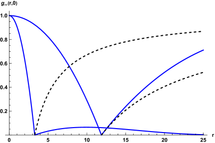
Figure 10: Metric component $g_{\tau\tau}(r,0)$ for $c_{G}=5.3$ ($h=11.9$) and 1.5 ($h=3.3$); $\kappa_{2}=1.240$. The corresponding Schwarzschild metrics are also shown (black, dashed).

The second derivative of $g_{\tau\tau}(r,0)$ at the horizon is independent of $c_{G}$ and given by

$$F^{\prime\prime}(h)=-24\,q_{1}\,.$$ (43)

Its negative sign ($-q_{1}<0$) matches the concavity of the curve in $r>h$, which its shares with the Schwarzschild form. For $\kappa_{2}=1.245$ with its larger $q_{1}$ the curve falls below that of Schwarzschild. (With the fit function $f_{\rm ch}(r)$ this curve has the wrong convex behavior.)

Assuming the Einstein equations to be valid in the effective sense, the condensate energy and pressure are given by the Einstein tensor, as in (6), which can be very conveniently calculated (for $\tau\neq 0$) using the software QERe [52]. When $\tau\to 0$ it becomes diagonal with energy density and pressures given by

$$8\pi G_{\rm N}\{\rho\,,\,p_{r}\,,\,p_{\theta}\,,\,p_{\phi}\}=\{-G^{\tau}_{\;\,\tau}\,,G^{r}_{\;\,r}\,,G^{\theta}_{\;\,\theta}\,,G^{\phi}_{\;\,\phi}\}\,.$$ (44)

In the exterior region, $r>h$, we find

$$G^{\tau}_{\;\,\tau}=G^{\theta}_{\;\,\theta}=G^{\phi}_{\;\,\phi} = -\frac{1}{r^{2}}\,\left[1+\frac{4(c_{G}p_{1}-q_{1}r)^{2}(c_{G}^{2}p_{0}p_{1}-2c_{G}(p_{1}+2p_{0}q_{1})r+5q_{1}r^{2})}{c_{G}^{2}(p_{1}-p_{0}q_{1})^{2}}\right]\,,$$ (45)

$$G^{r}_{\;\,r} = -\frac{3}{r^{2}}\left[1+\frac{4(c_{G}p_{0}-r)(c_{G}p_{1}-q_{1}r)^{3}}{c_{G}^{2}(p_{1}-p_{0}q_{1})^{2}})\right]\,,$$ (46)

In the interior region $0<r<h$,

$$G^{\tau}_{\;\,\tau} = -\frac{3}{c_{G}^{2}p_{0}^{2}}\,,$$ (47)

$$G^{r}_{\;\,r}=G^{\phi}_{\;\,\phi}=G^{\theta}_{\;\,\theta} = -\frac{1}{c_{G}^{2}p_{0}^{2}}+\frac{4p_{1}}{p_{0}}-4q_{1}\,,$$ (48)

independent of $r$. The interior energy-density $\rho$ is positive and the pressure $p$ is negative for $c_{G}<c_{G{\rm S}}$, as shown in figure 11. Figure 12 shows the case $c_{G}=c_{G{\rm S}}$, for which the interior pressure vanishes (note the difference in scale). For the case $c_{G}=c_{G0}$ the interior pressure is also positive, as shown in figure 13. In this case the curvature $R=-\sum_{\mu}G^{\mu}_{\;\,\mu}(r,0)$ vanishes in the interior and continuous at $r=h$.

Figure 11: Energy density $8\pi G_{\rm N}\rho$ (blue, positive) and pressure $8\pi G_{\rm N}\,p_{r}$ (red, negative) for $c_{G}=1.5$ ($h=3.3$).

Figure 12: As in figure 11 for $c_{G}$ in (42), $c_{G}=5.3$ ($h=12$). In this case the pressure vanishes in the interior $r<h$.

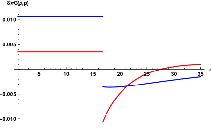
Figure 13: Energy density (blue) and pressure (red) as in figure 11 for $c_{G}=c_{G0}=7.5$ ($h=17$) in (27).

Discontinuities at $r=h$ may be expected from the discontinuous first derivative of $g_{\tau\tau}(r,0)$ at $r=h$, as evident in figure 10 and the different surface gravities $\kappa_{\pm}$ in (41). The Einstein tensor contains two derivatives of the metric and when these are both spatial a Dirac delta distribution will also be present. Using the Heaviside step function $\theta(x)$, $d\theta(x)/dx=\delta(x)$, $x\,\delta(x)=0$, and the expressions in problems 14.13 or 14.16 of [56], equations (38) – (41) lead to a contribution to the transverse pressure $p_{\theta}=p_{\phi}$,

$$\Delta p_{\phi} = \frac{1}{8\pi G_{\rm N}}\,\partial_{r}^{2}\left[(\kappa_{+}\theta(r-h)+\kappa_{-}\theta(h-r))\right]$$ (49)

$$= \frac{\Delta\kappa}{8\pi G_{\rm N}}\,\delta(r-h)\,,\quad\Delta\kappa=\kappa_{+}-\kappa_{-}>0\,.$$

On the other hand, one expects the scalar curvature invariant $R(r)$ to be continuous at the horizon; $R$ is equal to minus the trace of the Einstein tensor, and indeed continuous at $r=h=c_{G}\,p_{0}$ by (45)–(48). Since $R=8\pi G_{\rm N}(\rho-p_{r}-p_{\theta}-p_{\phi})$, there should also be a contribution to the energy density

$$\Delta\rho=\frac{\Delta\kappa}{4\pi G_{\rm N}}\,\delta(r-h)$$ (50)

which cancels $\Delta p_{\theta}+\Delta p_{\phi}$ in $R$. Integrated over the horizon this can be interpreted as a boundary layer surface tension [50].

The integrated Misner-Sharp mass at $\tau=0$ is by (37), (40), (44) and (47),

$$\lim_{r\to h^{-}}4\pi\int_{0}^{r}d\bar{r}\,r^{2}\rho=\frac{h}{2G_{\rm N}}\equiv M\,,$$ (51)

and the corresponding boundary layer contribution

$$M_{\rm layer}=\frac{h^{2}\Delta\kappa}{G_{\rm N}}\,.$$ (52)

The mass (51) has the Schwarzschild form which appears to support choosing $c_{G}=c_{G{\rm S}}$. The binding-energy estimate made in [38], $\sqrt{G_{\rm N}}\approx 8$ , was for $\kappa_{2}=1.255$ and one expects it to be larger with the present 1.240. Taking $\sqrt{G_{\rm N}}=10$ gives an idea of the order of magnitude in case $c_{G}=c_{G{\rm S}}$: $M\approx 0.06$, $M_{\rm layer}\approx 0.15$, in lattice units $\tilde{\ell}=1$.

VI Conclusions

The intuitive idea that the collapsed phase may tell us something about black holes stimulated a change of coordinates that showed an black hole at time zero, with a condensate in its interior, discontinuous and with delta shells at the horizon radius $h$, and decaying in the exterior region which was probed up to about $2h$. There are similarities with the gravastars in [50] and remnants [53]. Depending on the integration constant $c_{G}$ the pressure could be positive or negative but the energy was positive in all cases.

In the computation of the propagators, the origin was averaged over the volume (as occurs also in the quantum average), in a sampling approximation. On large volumes this might wash out black hole effects since the black hole is expected to reside near the singular structure. Perhaps a ‘center of mass’ selection as described in [6] should be used before taking the quantum average, albeit this would break the discrete remnant of diffeomorphism invariance in DT. The situation seems analogous to spontaneous symmetry breaking in field theory.

Of course, the importance of the results depends on corroboration by an approach to continuum and infinite volume limits. In the scenario using the measure term mentioned in the Introduction (section I), scaling ‘lines of constant physics’ should cross $\beta=0$ away from the phase boundary in order to be well in the collapsed phase.

The method of obtaining a metric based on the propagation of massless fields may also lead to a new validation of EDT’s elongated phase.

Appendix A EDT and metric from a volume-distance correlator

The EDT spacetimes used here are piece-wise flat manifolds consisting of equilateral 4-simplexes glued together at their 3-simplex boundaries, called ‘combinatorial triangulations’. The number of $i$-simplexes in these simplicial complexes is denoted by $N_{i}$, $i$=1,…,4. In the present study their topology is $S^{4}$. The volume of an $i$-simplex is given by

$$v_{i}=\frac{\ell^{i}\sqrt{i+1}}{i!\sqrt{2^{i}}}\,,$$ (53)

with $\ell$ the spacing between the lattice points. The centers of the 4-simplexes make up the dual lattice, with spacing $\tilde{\ell}=\ell/\sqrt{10}$. In the following the dual lattice will be important. Unless other wise indicated we shall be using units $\tilde{\ell}=1$.

Let $t$ denote a triangle, $t=1,\ldots,N_{2}$. The integral of the scalar curvature around a single triangle is given by [57, 58]

$$\int_{t}d^{4}x\,\sqrt{g}\,R=2\,v_{2}(2\pi-o_{t}\,\theta)\equiv R_{t}\,,$$ (54)

where $\theta=\arccos(1/4)$ and $o_{t}$ is the order of the triangle, the number of 4-simplexes containing $t$. Summing over all triangle contributions gives

$$\int d^{4}x\,\sqrt{g}\,R=\sum_{t}R_{t}=2v_{2}(2\pi\,N_{2}-10\theta\,N_{4})\,.$$ (55)

The Einstein-Hilbert action $S_{\rm EH}$ with bare parameters $G_{{\rm N}0}$ and $\Lambda_{0}$ becomes

$$\frac{1}{16\pi G_{{\rm N}0}}\int d^{4}x\,\sqrt{g}\,(2\Lambda_{0}-R)=\kappa_{4}N_{4}-\kappa_{2}N_{2}\,,$$ (56)

where

$$\kappa_{2}=\frac{v_{2}}{4\,G_{{\rm N}0}}\,,\quad\kappa_{4}=\frac{\Lambda_{0}v_{4}+10\theta v_{2}}{8\pi G_{{\rm N}0}}\,.$$ (57)

The partition functions are sums over triangulations $\mathcal{T}(N_{4})$ at fixed topology,

$$Z = \int Dg\,e^{-S_{\rm EH}}\to Z(\kappa_{2},\kappa_{4})\,,$$ (58)

$$Z(\kappa_{2},\kappa_{4}) = \sum_{N_{4}}e^{-\kappa_{4}N_{4}}Z(\kappa_{2},N_{4})\,,$$ (59)

$$Z(\kappa_{2},N_{4}) = \sum_{{\cal T}(N_{4})}\frac{1}{C(\mathcal{T})}\,e^{\kappa_{2}N_{2}}\,,$$ (60)

$$Z(\kappa_{2},\beta,N_{4}) = \sum_{{\cal T}(N_{4})}\frac{M(\mathcal{T},\beta)}{C(\mathcal{T})}\,e^{\kappa_{2}N_{2}}\,.$$ (61)

Here $C(\mathcal{T})$ is the order of the symmetry group (authomorphisms) that $\mathcal{T}$ may have, which is relevant for strong coupling expansions on small lattices [59, 8]. In (61) a ‘measure term’ [9] is inserted which introduces a third coupling parameter $\beta$,

$$M(\mathcal{T},\beta)=\prod_{t}o_{t}^{\beta}=\exp\left[\beta\sum_{t}\ln\left(\frac{2\pi}{\theta}-\frac{R_{t}}{2\theta v_{2}}\right)\right],$$ (62)

where we used (54). It depends logarithmically on the curvature but the product form shows that is still local.

We worked with the fixed-volume, ‘canonical’, partition function (60), i.e. $\beta=0$. Then the quantum average of observables $O$ is

$$\langle O\rangle=\frac{1}{Z(\kappa_{2},N_{4})}\sum_{{\cal T}(N_{4})}e^{\kappa_{2}N_{2}}\,O({\cal T})\,.$$ (63)

In particular, average scalar field propagators on $\mathcal{T}$ were computed by inverting a lattice version of the Laplace-Beltrami operator as in [36]. With $S^{4}$ topology this operator has an exact zero mode, the constant mode. Computations of propagators in four dimensions where pioneered in [1].

We call the average number of elementary 4-simplexes at dual lattice distance $r$ from an arbitrary origin the volume-distance correlator, $n(r)$. The average number of simplexes within distance $r$ is

$$N(r)=N(0)+\sum_{\bar{r}=1}^{r}n(\bar{r})\,,\quad N(0)=1\,,$$ (64)

in terms of which

$$n(r)=N(r)-N(r-1)\equiv N^{\prime}(r-1/2)\equiv\tilde{n}(r-1/2)\,.$$ (65)

Here $N^{\prime}$ is a discrete derivative and $\tilde{n}(r)$ is a shifted version of $n(r)$. These observables are compared with the volumes (2) of an isotropic space in the continuum. Typical examples are maximal symmetric spaces, which metrics were matched in [42] to volume-distance correlators at relatively small distances.

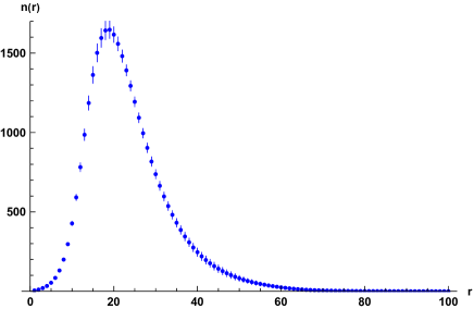
Figure 14: Volume-distance correlator $n(r)$ for $N_{4}=32000$, $\kappa_{2}=1.240$.

Figure 14 shows a collapsed-phase example relevant for the present work. It is fitted by the hyperbolic-sine form $c\,r_{0}^{3}\sinh[(r-s)/r_{0}]^{3}$ which corresponds to a 4D hyperbolic space with constant negative curvature $-12/r_{0}^{2}$, as follows from (25) when $a(r)=r_{0}\,\sinh(r/r_{0})$. The largest point in the fit domain, $2\leq r\leq 10$, is still smaller than the inflexion point of $n(r)$ near $r=13$. The fitted parameters are

$$c=0.093\,\quad s=-2.7\,,\quad r_{0}=10\,.$$ (66)

On the right of its maximum $n(r)$ is fitted by a Gaussian form $\exp(e_{0}-e_{1}\,r-e_{2}\,r^{2})$, which represents branched-polymer behavior at large $r$ [24, 42]. The fitted parameters are

$$e_{0}=9.05\,,\quad e_{1}=0.0635\,,\quad e_{2}=0.000609\,.$$ (67)

The transition region to branched polymer behavior appears to be broad. For definiteness, the smallest distance in the fit domain was chosen to be at the right inflexion point of $n(r)$, $r=25$. The volume of the region $r>25$ is a substantial fraction of the total volume: $(N_{4}-N(25))/N_{4}=0.34$.

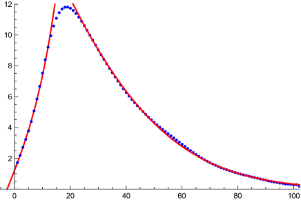
Figure 15: Central values $n(r)^{\frac{1}{3}}$ of the $n(r)$ data in figure 14 (blue dots); $c^{\frac{1}{3}}\,r_{0}\,\sinh[(r-s)/r_{0}]$ from the fit to $n(r)$ in the region $2\leq r\leq 10$ (red curve on the left flank) and $\exp[\frac{1}{3}(e_{0}-e_{1}\,r-e_{2}\,r^{2})]$ from the fit to $n(r)$ in the region $25\leq r\leq 110$.

Besides fitting $n(r)$ with constant-curvature forms, detailed scale factors $a(r)$ were also studied through interpolation of $n(r)^{1/3}$. Figure 15 shows $n(r)^{1/3}$ together with the above fits to the left and right flanks of $n(r)$. In the following $\tilde{n}(r)$ is used instead of $n(r)$ as it avoids having to discuss some discretization effects. For convenience an interpolation of $\tilde{n}(r)^{1/3}$ is denoted by $\tilde{n}_{1/3}(r)$. The lattice scale factor for a metric of the form (1) is proposed to be given by

$$a(r-\tilde{s})=c^{-1/3}\,\tilde{n}_{1/3}(r)\,,$$ (68)

where $c$ and $\tilde{s}$ are determined as follows: linear interpolation of and $\tilde{n}(3/2)^{1/3}$ and extrapolation into the region $r<1/2$ results in a zero at $r=\tilde{s}$, $\tilde{n}_{1/3}(\tilde{s})=0$, and $c$ follows from requiring $a(r)$ to vanish at $\tilde{s}$ with unit slope,

$$a(0)=0\,,\quad a^{\prime}(0)=1\,.$$ (69)

These requirements ensure that the space with scale factor $a(r)$ extended to $\tilde{s}$ has no conical singularity. Typically $\tilde{s}$ is negative with magnitude a few $\tilde{\ell}$, and the case in figure 14 the parameters come out with the shifted value of $s$ by about 1/2 compared to (66), $\tilde{s}=-3.1$, $c=0.11$ . Subsequently the discrete values of $\tilde{n}_{1/3}(r)$ at half-integer values are interpolated by a polynomial of sufficiently high order.

To enable using continuum formulas, such as $\int d\Omega_{3}=2\pi^{2}$ when calculating a volume as in (2), $a$ and $r$ were scaled in [42] by a factor $\lambda$ and the resulting quantities dubbed ‘continuum’, indicated by a subscript ‘c’,

$$r_{\rm c}=\lambda\,(r-s)\,,\quad a_{\rm c}(r_{\rm c})=\lambda\,a(r-s)\,,\quad r_{0{\rm c}}=\lambda\,r_{0}\,,$$ (70)

The factor $\lambda$ was defined in [42] as

$$\lambda^{4}=\frac{v_{4}c}{2\pi^{2}}\,,$$ (71)

which gives $\lambda=0.34$ for the case in figure 14. An $r$-dependent $\lambda(r)$ can be defined by comparing the continuum volume $V_{\rm c}(r_{\rm c})$ with the lattice $N(r)v_{4}$:

$$V_{\rm c}(r_{\rm c}) = 2\pi^{2}\int_{0}^{r_{\rm c}}dr_{\rm c}\,a_{\rm c}(r_{\rm c})^{3}=2\pi^{2}\frac{\lambda(r)^{4}}{c}\,\int_{\tilde{s}}^{r}d\bar{r}\,\tilde{n}_{1/3}(\bar{r})^{3}$$ (72)

$$= N(r)v_{4}\,\Rightarrow\lambda(r)^{4}=\lambda^{4}\,\frac{N(r)}{\int_{\tilde{s}}^{r}d\bar{r}\,\tilde{n}_{1/3}(\bar{r})^{3}}\,.$$

The ratio $\lambda(r)^{4}/\lambda^{4}$ is plotted in figure 16; it is close to unity for $r\gtrsim 5$.

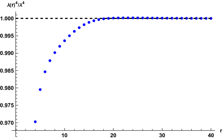
Figure 16: The ratio $\lambda(r)^{4}/\lambda^{4}$ in (72); $N_{4}=32$ k, $\kappa_{2}=1.240$.

The resulting scale factor $a_{\rm c}(r_{\rm c})$ can be used to compute the curvature using (25), with $a(r)\to a_{\rm c}(r_{\rm c})$. Judging results, it is convenient to use the original units, i.e. $R=\lambda^{2}R_{\rm c}$. The unscaled $R(r-\tilde{s})$ is plotted in figure 17 (black curve). It shows negative curvature around $r=6$ and a change to positive curvature already at $r=11$. The horizontal black dashed line is $-12/r_{0}^{2}$ with curvature radius (66) from the fit with the hyperbolic-sine function.

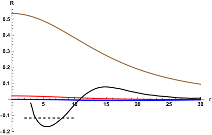
Figure 17: Wiggly black curve: curvature $R(r-\tilde{s})$; horizontal black dashed line $-12/r_{0}^{2}$ with $r_{0}=10$; small magnitude curves (red and blue) are the same as in figure 9); large positive brown curve corresponds to $a(r)=c_{G}f_{\rm rat}(r)$, $c_{G}=1.46$.

For comparison, also shown are the curvatures obtained from the propagator metric $a(r)=c_{G}\,a_{G}(r)$ with the rational function fit $a_{G}(r)=f_{\rm rat}(r)$, $c_{G}=c_{G{\rm S}}$ and $c_{G}=c_{G0}$ (which were shown on a smaller scale in figure 9). The large positive curve (brown) represents the case $c_{G}=1.46$, a result of the following considerations:

As mentioned at the end of section IV a possible choice of the integration constant $c_{G}$ can be made by comparing the volume within an average ‘blob’ size of radius $r_{\rm blob}$ with the simplex-volume within that radius, $N(r_{\rm blob})v_{4}$. A candidate for $r_{\rm blob}$ is the inflexion point $r_{\rm infl}$ in $n(r)$ beyond which the branched polymer fit shown in figure 15 was applied, $r_{\rm infl}=25$. Defining an $r$-dependent $c_{G}(r)$,

$$c_{G}(r)=\left[\frac{N(r)\,v_{4}}{2\pi^{2}\int_{0}^{r}d\bar{r}\,a_{G}(\bar{r})^{3}}\right]^{1/3}\,,$$ (73)

the sensitivity of $c_{G}$ to $r=r_{\rm blob}$ can be judged from figure 18. With the fit function $f_{\rm rat}(r)$ this gives $c_{G}(25)=1.46$ for $r_{\rm blob}=25$, the maximal value is $c_{G}(20)=1.55$.

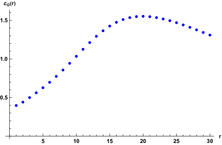
Figure 18: Plot of $c_{G}(r)$ in (73).

References

- Agishtein and Migdal [1992] M. E. Agishtein and A. A. Migdal, Simulations of four-dimensional simplicial quantum gravity, Mod. Phys. Lett. A7, 1039 (1992).
- Ambjorn and Jurkiewicz [1992] J. Ambjorn and J. Jurkiewicz, Four-dimensional simplicial quantum gravity, Phys. Lett. B278, 42 (1992).
- Bilke and Thorleifsson [1999] S. Bilke and G. Thorleifsson, Simulating four-dimensional simplicial gravity using degenerate triangulations, Phys. Rev. D 59, 124008 (1999), arXiv:hep-lat/9810049 .
- Thorleifsson [1999] G. Thorleifsson, Lattice gravity and random surfaces, Nucl. Phys. B Proc. Suppl. 73, 133 (1999), arXiv:hep-lat/9809131 .
- Ambjorn et al. [1999a] J. Ambjorn, K. N. Anagnostopoulos, and J. Jurkiewicz, Abelian gauge fields coupled to simplicial quantum gravity, JHEP 08, 016, arXiv:hep-lat/9907027 .
- Ambjorn et al. [2013] J. Ambjorn, L. Glaser, A. Goerlich, and J. Jurkiewicz, Euclidian 4d quantum gravity with a non-trivial measure term, JHEP 10, 100, arXiv:1307.2270 [hep-lat] .
- Laiho et al. [2017] J. Laiho, S. Bassler, D. Coumbe, D. Du, and J. Neelakanta, Lattice Quantum Gravity and Asymptotic Safety, Phys. Rev. D 96, 064015 (2017), arXiv:1604.02745 [hep-th] .
- Bilke et al. [1998a] S. Bilke, Z. Burda, A. Krzywicki, B. Petersson, J. Tabaczek, and G. Thorleifsson, 4d simplicial quantum gravity interacting with gauge matter fields, Phys. Lett. B418, 266 (1998a), arXiv:hep-lat/9710077 .
- Bilke et al. [1998b] S. Bilke, Z. Burda, A. Krzywicki, B. Petersson, J. Tabaczek, and G. Thorleifsson, 4d simplicial quantum gravity: Matter fields and the corresponding effective action, Phys. Lett. B432, 279 (1998b), arXiv:hep-lat/9804011 .
- Coumbe and Laiho [2015] D. Coumbe and J. Laiho, Exploring Euclidean Dynamical Triangulations with a Non-trivial Measure Term, JHEP 04, 028, arXiv:1401.3299 [hep-th] .
- Bruegmann and Marinari [1993] B. Bruegmann and E. Marinari, 4-d simplicial quantum gravity with a nontrivial measure, Phys.Rev.Lett. 70, 1908 (1993), arXiv:hep-lat/9210002 [hep-lat] .
- Asaduzzaman and Catterall [2022] M. Asaduzzaman and S. Catterall, Euclidean Dynamical Triangulations Revisited, (2022), arXiv:2207.12642 [hep-lat] .
- Bialas et al. [1996] P. Bialas, Z. Burda, A. Krzywicki, and B. Petersson, Focusing on the fixed point of 4d simplicial gravity, Nucl. Phys. B472, 293 (1996), arXiv:hep-lat/9601024 .
- de Bakker [1996] B. V. de Bakker, Further evidence that the transition of 4D dynamical triangulation is 1st order, Phys. Lett. B389, 238 (1996), arXiv:hep-lat/9603024 .
- Rindlisbacher and de Forcrand [2015] T. Rindlisbacher and P. de Forcrand, Euclidean Dynamical Triangulation revisited: is the phase transition really 1st order? (extended version), JHEP 1505, 138, arXiv:1503.03706 [hep-lat] .
- Ambjorn et al. [2012] J. Ambjorn, A. Goerlich, J. Jurkiewicz, and R. Loll, Nonperturbative Quantum Gravity, Phys. Rept. 519, 127 (2012), arXiv:1203.3591 [hep-th] .
- Loll [2020] R. Loll, Quantum Gravity from Causal Dynamical Triangulations: A Review, Class. Quant. Grav. 37, 013002 (2020), arXiv:1905.08669 [hep-th] .
- Ambjorn [2022] J. Ambjorn, Lattice Quantum Gravity: EDT and CDT (2022) arXiv:2209.06555 [hep-lat] .
- Ambjorn et al. [2014] J. Ambjorn, A. Görlich, J. Jurkiewicz, A. Kreienbuehl, and R. Loll, Renormalization Group Flow in CDT, Class. Quant. Grav. 31, 165003 (2014), arXiv:1405.4585 [hep-th] .
- Ambjorn et al. [2016] J. Ambjorn, D. Coumbe, J. Gizbert-Studnicki, and J. Jurkiewicz, Searching for a continuum limit in causal dynamical triangulation quantum gravity, Phys. Rev. D 93, 104032 (2016), arXiv:1603.02076 [hep-th] .
- Gizbert-Studnicki [2023] J. Gizbert-Studnicki, Semiclassical and Continuum Limits of Four-Dimensional CDT (2023) arXiv:2301.06068 [hep-th] .
- Hamber [2019] H. W. Hamber, Vacuum Condensate Picture of Quantum Gravity, Symmetry 11, 87 (2019), arXiv:1707.08188 [hep-th] .
- Rocek and Williams [1981] M. Rocek and R. M. Williams, Quantum Regge Calculus, Phys. Lett. B 104, 31 (1981).
- Ambjorn and Jurkiewicz [1995] J. Ambjorn and J. Jurkiewicz, Scaling in four-dimensional quantum gravity, Nucl. Phys. B451, 643 (1995), arXiv:hep-th/9503006 .
- Hotta et al. [1996] T. Hotta, T. Izubuchi, and J. Nishimura, Singular Vertices in the Strong Coupling Phase of Four-Dimensional Simplicial Gravity, Nucl. Phys. Proc. Suppl. 47, 609 (1996), arXiv:hep-lat/9511023 .
- Hotta et al. [1995] T. Hotta, T. Izubuchi, and J. Nishimura, Singular vertices in the strong coupling phase of four-dimensional simplicial gravity, Prog.Theor.Phys. 94, 263 (1995), arXiv:hep-lat/9709073 [hep-lat] .
- Catterall et al. [1996] S. Catterall, G. Thorleifsson, J. B. Kogut, and R. Renken, Singular Vertices and the Triangulation Space of the D- sphere, Nucl. Phys. B468, 263 (1996), arXiv:hep-lat/9512012 .
- Catterall et al. [1998] S. Catterall, R. Renken, and J. B. Kogut, Singular structure in 4-D simplicial gravity, Phys.Lett. B416, 274 (1998), arXiv:hep-lat/9709007 [hep-lat] .
- Ambjorn et al. [1999b] J. Ambjorn, M. Carfora, D. Gabrielli, and A. Marzuoli, Crumpled triangulations and critical points in 4-D simplicial quantum gravity, Nucl. Phys. B 542, 349 (1999b), arXiv:hep-lat/9806035 .
- Hikami [2018] S. Hikami, Conformal Bootstrap Analysis for Single and Branched Polymers, PTEP 2018, 123I01 (2018), arXiv:1708.03072 [hep-th] .
- Poland et al. [2019] D. Poland, S. Rychkov, and A. Vichi, The Conformal Bootstrap: Theory, Numerical Techniques, and Applications, Rev. Mod. Phys. 91, 015002 (2019), arXiv:1805.04405 [hep-th] .
- Maldacena [1998] J. M. Maldacena, The Large N limit of superconformal field theories and supergravity, Adv. Theor. Math. Phys. 2, 231 (1998), arXiv:hep-th/9711200 .
- Witten [1998a] E. Witten, Anti-de Sitter space and holography, Adv. Theor. Math. Phys. 2, 253 (1998a), arXiv:hep-th/9802150 .
- Witten [1998b] E. Witten, Anti-de Sitter space, thermal phase transition, and confinement in gauge theories, Adv. Theor. Math. Phys. 2, 505 (1998b), arXiv:hep-th/9803131 .
- Smit [2002] J. Smit, Introduction to quantum fields on a lattice: A robust mate, Cambridge Lect. Notes Phys. 15 (2002), [Erratum: https://www.researchgate.net/profile/Jan-Smit-7].
- de Bakker and Smit [1997] B. V. de Bakker and J. Smit, Gravitational binding in 4D dynamical triangulation, Nucl. Phys. B484, 476 (1997), arXiv:hep-lat/9604023 .
- de Bakker and Smit [1994] B. de Bakker and J. Smit, Euclidean gravity attracts, Nucl. Phys. B Proc. Suppl. 34, 739 (1994), arXiv:hep-lat/9311064 .
- Smit [2021] J. Smit, Three models of non-perturbative quantum-gravitational binding, (2021), arXiv:2101.01028 [gr-qc] .
- Dai et al. [2021] M. Dai, J. Laiho, M. Schiffer, and J. Unmuth-Yockey, Newtonian binding from lattice quantum gravity, Phys. Rev. D 103, 114511 (2021), arXiv:2102.04492 [hep-lat] .
- Bassler et al. [2021] S. Bassler, J. Laiho, M. Schiffer, and J. Unmuth-Yockey, The de Sitter Instanton from Euclidean Dynamical Triangulations, Phys. Rev. D 103, 114504 (2021), arXiv:2103.06973 [hep-lat] .
- de Bakker and Smit [1995] B. V. de Bakker and J. Smit, Curvature and scaling in 4-d dynamical triangulation, Nucl. Phys. B439, 239 (1995), arXiv:hep-lat/9407014 .
- Smit [2013] J. Smit, Continuum interpretation of the dynamical-triangulation formulation of quantum Einstein gravity, JHEP 08, 016, [Erratum: JHEP 09, 048 (2015)], arXiv:1304.6339 [hep-lat] .
- Smit [1997] J. Smit, Remarks on the quantum gravity interpretation of 4D dynamical triangulation, Nucl. Phys. Proc. Suppl. 53, 786 (1997), arXiv:hep-lat/9608082 .
- de Bakker and Smit [1996a] B. V. de Bakker and J. Smit, Curvature in the crumpled phase of 4D dynamical triangulation, unpublished draft (1996a).
- de Bakker [1995] B. V. de Bakker, Simplicial quantum gravity, (1995), arXiv:hep-lat/9508006 .
- Chapline et al. [2003] G. Chapline, E. Hohlfeld, R. B. Laughlin, and D. I. Santiago, Quantum phase transitions and the breakdown of classical general relativity, Int. J. Mod. Phys. A 18, 3587 (2003), arXiv:gr-qc/0012094 .
- Mazur and Mottola [2001] P. O. Mazur and E. Mottola, Gravitational condensate stars: An alternative to black holes, (2001), arXiv:gr-qc/0109035 .
- Mazur and Mottola [2004] P. O. Mazur and E. Mottola, Gravitational vacuum condensate stars, Proc. Nat. Acad. Sci. 101, 9545 (2004), arXiv:gr-qc/0407075 .
- Cattoen et al. [2005] C. Cattoen, T. Faber, and M. Visser, Gravastars must have anisotropic pressures, Class. Quant. Grav. 22, 4189 (2005), arXiv:gr-qc/0505137 .
- Mazur and Mottola [2015] P. O. Mazur and E. Mottola, Surface tension and negative pressure interior of a non-singular ‘black hole’, Class. Quant. Grav. 32, 215024 (2015), arXiv:1501.03806 [gr-qc] .
- Simpson and Visser [2019] A. Simpson and M. Visser, Regular black holes with asymptotically Minkowski cores, Universe 6, 8 (2019), arXiv:1911.01020 [gr-qc] .
- Shoshany [2021] B. Shoshany, OGRe: An Object-Oriented General Relativity Package for Mathematica, J. Open Source Softw. 6, 3416 (2021), arXiv:2109.04193 [cs.MS] .
- Bonanno and Saueressig [2022] A. Bonanno and F. Saueressig, Stability properties of Regular Black Holes, (2022), arXiv:2211.09192 [gr-qc] .
- de Bakker and Smit [1996b] B. V. de Bakker and J. Smit, Curvature in the crumpled phase of 4D dynamical triangulation, unpublished draft (1996b).
- Gibbons and Hawking [1977] G. W. Gibbons and S. W. Hawking, Action Integrals and Partition Functions in Quantum Gravity, Phys. Rev. D 15, 2752 (1977).
- Misner et al. [1973] C. W. Misner, K. S. Thorne, and J. A. Wheeler, Gravitation (W. H. Freeman, San Francisco, 1973).
- Cheeger et al. [1984] J. Cheeger, W. Muller, and R. Schrader, On the Curvature of Piecewise Flat Spaces, Commun.Math.Phys. 92, 405 (1984).
- Friedberg and Lee [1984] R. Friedberg and T. Lee, Derivation of Regge’s Action From Einstein’s Theory of General Relativity, Nucl.Phys. B242, 145 (1984).
- Bilke et al. [1999] S. Bilke, Z. Burda, A. Krzywicki, B. Petersson, K. Petrov, J. Tabaczek, and G. Thorleifsson, The Strong coupling expansion in simplicial quantum gravity, Nucl. Phys. B Proc. Suppl. 73, 798 (1999), arXiv:hep-lat/9809088 .