The #DNN-Verification Problem:
Counting Unsafe Inputs for Deep Neural Networks

Abstract

Deep Neural Networks are increasingly adopted in critical tasks that require a high level of safety, e.g., autonomous driving. While state-of-the-art verifiers can be employed to check whether a DNN is unsafe w.r.t. some given property (i.e., whether there is at least one unsafe input configuration), their yes/no output is not informative enough for other purposes, such as shielding, model selection, or training improvements. In this paper, we introduce the #DNN-Verification problem, which involves counting the number of input configurations of a DNN that result in a violation of a particular safety property. We analyze the complexity of this problem and propose a novel approach that returns the exact count of violations. Due to the #P-completeness of the problem, we also propose a randomized, approximate method that provides a provable probabilistic bound of the correct count while significantly reducing computational requirements. We present experimental results on a set of safety-critical benchmarks that demonstrate the effectiveness of our approximate method and evaluate the tightness of the bound.

1 Introduction

In recent years, the success of Deep Neural Networks (DNNs) in a wide variety of fields (e.g., games playing, speech recognition, and image recognition) has led to the adoption of these systems also in safety-critical contexts, such as autonomous driving and robotics, where humans safety and expensive hardware can be involved. A popular and successful example is “ACAS Xu”, an airborne collision avoidance system for aircraft based on a DNN controller, which is now a standard DNN-verification benchmark.

A DNN is a non-linear function that maps a point in the input space to an output that typically represents an action or a class (respectively, for control and classification tasks). A crucial aspect of these DNNs lies in the concept of generalization. A neural network is trained on a finite subset of the input space, and at the end of this process, we expect it to find a pattern that allows making decisions in contexts never seen before. However, even networks that empirically perform well on a large test set can react incorrectly to slight perturbations in their inputs Szegedy et al. (2013). While this is a negligible concern in simulated and controlled environments, it can potentially lead to catastrophic consequences for real safety-critical tasks, possibly endangering human health. Consequently, in recent years, part of the scientific communities devoted to machine learning and formal methods have joined efforts to develop DNN-Verification techniques that provide formal guarantees on the behavior of these systems Liu et al. (2021)Katz et al. (2021).

Given a DNN and a safety property, a DNN verification tool should ideally either ensure that the property is satisfied for all the possible input configurations or identify a specific example (e.g., adversarial configuration) that violates the requirements. Given these complex functions’ non-linear and non-convex nature, verifying even simple properties is proved to be an NP-complete problem Katz et al. (2017). In literature, several works try to solve the problem efficiently either by satisfiability modulo theories (SMT) solvers Liu et al. (2021)Katz et al. (2019) or by interval propagation methods Wang et al. (2021).

Although these methods show promising results, the current formulation, widely adopted for almost all the approaches, considers only the decision version of the formal verification problem, with the solution being a binary answer whose possible values are typically denoted SAT or UNSAT. SAT indicates that the verification framework found a specific input configuration, as a counterexample, that caused a violation of the requirements. UNSAT, in contrast, indicates that no such point exists, and then the safety property is formally verified in the whole input space. While an UNSAT answer does not require further investigations, a SAT result hides additional information and questions. For example, how many of such adversarial configurations exist in the input space? How likely are these misbehaviors to happen during a standard execution? Can we estimate the probability of running into one of these points? These questions can be better dealt with in terms of the problem of counting the number of violations to a safety property, a problem that might be important also in other contexts: (i) model selection: a counting result allows ranking a set of models to select the safest one. This model selection is impossible with a SAT or UNSAT type verifier, which does not provide any information to discriminate between two models which have both been found to violate the safety condition for at least one input configuration. (ii) guide the training: knowing the total count of violations for a particular safety property can help guiding the training of a deep neural network in a more informed fashion, for instance, minimizing this number over the training process. (iii) estimating the probability of error: the ratio of the total number of violations over the size of the input space provides an estimate of the probability of committing an unsafe action given a specific safety property.

Furthermore, by enumerating the violation points, it is possible to perform additional safety-oriented operations, such as: (iv) shielding: given the set of input configurations that violate a given safety property, we could adopt a more informative shielding mechanism that prevents unsafe actions.(v) enrich the training phase: if we can enumerate the violation configurations, we could add these configurations to the training (or to a memory buffer in deep reinforcement learning setup) to improve the training phase in a safe-oriented fashion. Motivated by the above questions and applications, previous works Baluta et al. (2019)Zhang et al. (2021)Ghosh et al. (2021) propose a quantitative analysis of neural networks, focusing on a specific subcategory of these functions, i.e., Binarized Neural Networks (BNN). However, violation points are generally not preserved in the binarization of a DNN to a BNN nor conversely in the relaxation of a BNN to a DNN Zhang et al. (2021).

To this end, in this paper, we introduce the #DNN-Verification problem, which is the extension of the decision DNN-Verification problem to the corresponding counting version. Given a general deep neural network (with continuous values) and a safety property, the objective is to count the exact number of input configurations that violate the specific requirement. We analyze the complexity of this problem and propose two solution approaches. In particular, in the first part of the paper, we propose an algorithm that is guaranteed to find the exact number of unsafe input configurations, providing a detailed theoretical analysis of the algorithm’s complexity. The high-level intuition behind our method is to recursively shrink the domain of the property, exploiting the SAT or UNSAT answer of a standard formal verifier to drive the expansion of a tree that tracks the generated subdomains. Interestingly, our method can rely on any formal verifier for the decision problem, taking advantage of all the improvements to state-of-the-art and, possibly, to novel frameworks. As the analysis shows, our algorithm requires multiple invocations of the verification tool, resulting in significant overhead and becoming quickly unfeasible for real-world problems. For this reason, inspired by the work of Gomes et al. (2007) on #SAT, we propose an approximation algorithm for #DNN-Verification, providing provable (probabilistic) bounds on the correctness of the estimation.

In more detail, in this paper, we make the following contribution to the state-of-the-art:

• We propose an exact count formal algorithm to solve #DNN-verification, that exploits state-of-the-art decision tools as backends for the computation.

• We present CountingProVe, a novel approximation algorithm for #DNN-verification, that provides a bounded confidence interval for the results.

• We evaluate our algorithms on a standard benchmark, ACAS Xu, showing that CountingProVe is scalable and effective also for real-world problems.

To the best of our knowledge, this is the first study to present #DNN-verification, the counting version of the decision problem of the formal verification for general neural networks without converting the DNN into a CNF.

2 Preliminaries

Deep Neural Networks (DNNs) are processing systems that include a collection of connected units called neurons, which are organized into one or more layers of parameterized non-linear transformations. Given an input vector, the value of each next hidden node in the network is determined by computing a linear combination of node values from the previous layer and applying a non-linear function node-wise (i.e., the activation function). Hence, by propagating the initial input values through the subsequent layers of a DNN, we obtain either a label prediction (e.g., for image classification tasks) or a value representing the index of an action (e.g., for a decision-making task).

Figure 1: A simple example of a DNN $\mathcal{N}$ that will be used as a running example throughout the paper.

Fig. 1 shows a concrete example of how a DNN computes the output. Given an input vector $V_{1}=[1,0]^{T}$, the weighted sum layer computes the value $V_{2}=[+5,-1]^{T}$. This latter is the input for the so-called activation function Rectified Linear Unit (ReLU), which computes the following transformation, $y=ReLU(x)=\max(0,x)$. Hence, the result of this activated layer is the vector $V_{3}=[+5,0]^{T}$. Finally, the network’s single output is again computed as a weighted sum, giving us the value $-5$.

2.1 The DNN-Verification Problem

An instance of the DNN-Verification problem (in its standard decision form) is given by a trained DNN $\mathcal{N}$ together with a safety property, typically expressed as an input-output relationship for $\mathcal{N}$ Liu et al. (2021). In more detail, a property is a tuple that consists of a precondition, expressed by a predicate $\mathcal{P}$ on the input, and a postcondition, expressed by a predicate $\mathcal{Q}$ on the output of $\mathcal{N}$. In particular, $\mathcal{P}$ defines the possible input values we are interested in—aka the input configurations—(i.e., the domain of the property), while $\mathcal{Q}$ represents the output results we aim to guarantee formally for at least one of the inputs that satisfy $\mathcal{P}.$ Then, the problem consists of verifying whether there exists an input configuration in $\mathcal{P}$ that, when fed to the DNN $\mathcal{N}$, produces an output satisfying $\mathcal{Q}$.

Definition 1 (DNN-Verification Problem).

a

Input: A tuple $\mathcal{R}=\langle\mathcal{N},\mathcal{P},\mathcal{Q}\rangle$, where $\mathcal{N}$ is a trained DNN, $\mathcal{P}$ is precondition on the input, and $\mathcal{Q}$ a postcondition on the output.

Output: SAT if $\exists\;x\;|\;\mathcal{P}(x)\wedge\mathcal{Q}(\mathcal{N}(x))$ and UNSAT otherwise, indicating that no such $x$ exists.

As an example of how this problem can be employed for checking the existence of unsafe input configurations for a DNN, suppose we aim to verify that the DNN $\mathcal{N}$ of Fig. 1, for any input in the interval $[0,1]$, outputs a value greater than or equal 0. Hence, we define $\mathcal{P}$ as the predicate on the input vector ${\bf v}=(v^{1}_{1},v^{1}_{2})$ which is true iff ${\bf v}\in[0,1]\times[0,1]$, and $\mathcal{Q}$ as the predicate on the output $v_{4}^{1}$ which is true iff $v_{4}^{1}=\mathcal{N}(v^{1}_{1},v^{1}_{2})<0,$ that is we set $\mathcal{Q}$ to be the negation of our desired property. Then, solving the DNN-Verification Problem on the instance $(\mathcal{N},\mathcal{P},\mathcal{Q})$ we get SAT iff there is counterexample that violates our property.

Since for the input vector ${\bf v}=(1,0)$ (also reported in Fig. 1), the output of $\mathcal{N}$ is $<0$, in the example, the result of the DNN-Verification Problem (with the postcondition being the negated of the desired property) is SAT, meaning that there exists at least a single input configuration $(v^{1}_{1},v^{1}_{2})$ that satisfies $\mathcal{P}$ and for which $\mathcal{N}(v^{1}_{1},v^{1}_{2})<0$. As a result, we can say that the network is not safe for the desired property.

3 #DNN-Verification and Exact Count

In this section, we first provide a formal definition for #DNN-Verification; hence, we propose an algorithm to solve the problem by exploiting any existing formal verification tool. Finally, we proceed with a theoretical discussion on the complexity of the problem, highlighting the need for approximate approaches.

3.1 Problem Formulation

Given a tuple $\mathcal{R}=\langle\mathcal{N},\mathcal{P},\mathcal{Q}\rangle$, as in Definition 1, we let $\Gamma(\mathcal{R})$ denote the set of all the input configurations for $\mathcal{N}$ satisfying the property defined by $\mathcal{P}$ and $\mathcal{Q},$ i.e.

$$\Gamma(\mathcal{R})=\Bigg{\{}x\;\big{|}\;\mathcal{P}(x)\wedge\mathcal{Q}(\mathcal{N}(x))\Bigg{\}}$$

Then, the #DNN-Verification consists of computing the cardinality of $\Gamma(\mathcal{R}).$

Definition 2 (#DNN-Verification Problem).

a

Input: A tuple $\mathcal{R}=\langle\mathcal{N},\mathcal{P},\mathcal{Q}\rangle$, as in Definition 1.

Output: $|\Gamma(\mathcal{R})|$

For the purposes discussed in the introduction, rather than the cardinality of $\Gamma(\mathcal{R})$, it is more useful to define the problem in terms of the ratio between the cardinality of $\Gamma$ and the cardinality of the set of inputs satisfying $\mathcal{P}.$ We refer to this ratio as the violation rate (VR), and study the result of the #DNN-Verification problem in terms of this equivalent measure.

Definition 3 (Violation Rate (VR)).

Given an instance of the DNN-Verification problem $\mathcal{R}=\langle\mathcal{N},\mathcal{P},\mathcal{Q}\rangle$ we define the violation rate as

$$VR=\frac{|\Gamma(\mathcal{R})|}{\lvert\{x\;|\;\mathcal{P}(x)\}\lvert}$$

Although, in general, DNNs can handle continuous spaces, in the following sections (and for the analysis of the algorithms), without loss of generality, we assume the input space to be discrete. We remark that for all practical purposes, this is not a limitation since we can assume that the discretization is made to the maximum resolution achievable with the number of decimal digits a machine can represent. It is crucial to point out that discretization is not a requirement of the approaches proposed in this work. In fact, supposing to have a backend that can deal with continuous values, our solutions would not require such discretization.

3.2 Exact Count Algorithm for #DNN-Verification

We now present an algorithm to solve the exact count of #DNN-Verification.

The algorithm recursively splits the input space into two parts of equal size as long as it contains both a point that violates the property (i.e., $(\mathcal{N},\mathcal{P},\mathcal{Q})$ is a SAT-instance for DNN-Verification problem) and a point that satisfies it (i.e., $(\mathcal{N},\mathcal{P},\neg\mathcal{Q}$) is a SAT-instance for DNN-Verification problem). The leaves of the recursion tree of this procedure correspond to a partition of the input space into parts where the violation rate is either 0 or 1. Therefore, the overall violation rate is easily computable by summing up the sizes of the subinput spaces in the leaves of violation rate 1.

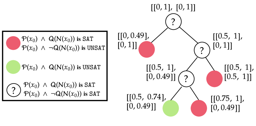
Figure 2: Example execution of exact count for a particular $\mathcal{N}$ and safety property (assuming a discretization factor of $0.01$).

Fig. 2 shows an example of the execution of our algorithm for the DNN and the safety property presented in Sec. 2. We want to enumerate the total number of input configurations ${\bf v}=(v_{1}^{1},v_{1}^{2})$ where both $v_{1}^{1}$ and $v_{1}^{2}$ satisfy $\mathcal{P}$ (i.e., they lie in the interval $[0,1]$) and such that the output $v^{1}_{4}=\mathcal{N}({\bf v})$ is a value strictly less than 0, i.e., ${\bf v}$ violates the safety property.

The algorithm starts with the whole input space and checks if at least one point exists that outputs a value strictly less than zero. The exact count method checks the predicate $\exists x\mid\mathcal{P}(x)\wedge\mathcal{Q}(\mathcal{N}(x))$ with a verification tool for the decision problem. If the result is UNSAT, then the property holds in the whole input space, and the algorithm returns a VR of $0\%$. Otherwise, if the verification tool returns SAT, at least one single violation point exists, but we cannot assert how many similar configurations exist in the input space. To this end, the algorithm checks another property equivalent to the original one, thus negating the postcondition (i.e., $\neg\mathcal{Q}=v_{1}^{4}\geq 0$). Here, we have two possible outcomes:

• $\mathcal{P}(x_{0})\wedge\neg\mathcal{Q}(\mathcal{N}(x_{0}))$ is UNSAT implies that all possible $x_{0}=(v_{1}^{1},v_{1}^{2})$ that satisfy $\mathcal{P}$, output a value strictly less than 0, violating the safety property. Hence, the algorithm returns a 100% of VR in the input area represented by $\mathcal{P}$. This situation is depicted with the red circle in Fig. 2.

• $\mathcal{P}(x_{0})\wedge\neg\mathcal{Q}(\mathcal{N}(x_{0}))$ is SAT implies that there is at least one input configuration ${\bf v}=(v_{1}^{1},v_{1}^{2})$ satisfying $\mathcal{P}$ and such that $\mathcal{N}({\bf v})\geq 0.$ Therefore, the algorithm cannot assert anything about the violated portion of the area since there are some input points on which $\mathcal{N}$ generates outputs greater or equal to zero and some others that generate a result strictly less than zero. Hence, the procedure splits the input space into two parts, as depicted in Fig. 2.

This process is repeated until the algorithm reaches one of the base cases, such as a situation in which either $\mathcal{P}(x)\wedge\mathcal{Q}(\mathcal{N}(x))$ is not satisfiable (i.e., all the current portion of the input space is safe), represented by a green circle in Fig.2), or $\mathcal{P}(x)\wedge\neg\mathcal{Q}(\mathcal{N}(x))$ is not satisfiable (i.e., the whole current portion of the input space is unsafe), represented by a red circle. Note that the option of obtaining UNSAT on both properties is not possible.

Finally, the algorithm of exact count returns the VR as the ratio between the unsafe areas (i.e., the red circles) and the original input area. In the example of Fig. 2, assuming a 2-decimal-digit discretization, we obtain a total number of violation points equal to $8951$. Normalizing this value by the initial total number of points ($10201$), and considering the percentage value, we obtain a final VR of $87.7\%$. Moreover, the Violation Rate can also be interpreted as the probability of violating a safety property using a particular DNN $\mathcal{N}$. In more detail, uniformly sampling $10$ random input vectors for our DNN $\mathcal{N}$ in the intervals described by $\mathcal{P}$, $8$ over $10$ with high probability violates the safety property.

3.3 Hardness of #DNN-Verification

It is known that finding even just one input configuration (also referred to as violation point) that violates a given safety property is computationally hard since the DNN-Verification problem is NP-Complete Katz et al. (2017). Hence, counting and enumerating all the violation points is expected to be an even harder problem.

Theorem 1.

The #DNN-Verification is #P-Complete.

Note that, in general, the counting version of an NP-complete problem is not necessarily #P-complete. We are able to prove Theorem 1 by showing that the hardness proof for DNN-Verification in Katz et al. (2017) provides a bijection between an assignment that satisfies a 3-CNF formula and a violation point in given input space (we include the details is in the supplementary material). Hence, #DNN-Verification turns out to be #P-Complete as #3-SAT Valiant (1979).

4 CountingProVe for Approximate Count

In view of the #P-completeness of the #DNN-Verification problem, it is not surprising that the time complexity of the algorithm for the exact count worsens very fast when the size of the instance increases. In fact also moderately large networks are intractable with this approach. To overcome these limitations while still providing guarantees on the quality of the results, we propose a randomized-approximation algorithm, CountingProVe (presented in Algorithm 1).

To understand the intuition behind our approach, consider Fig. 2. If we could assume that each split distributed the violation points evenly in the two subinstances it produces, for computing the number of violation points in the whole input space it would be enough to compute the number of violation points in the subspace of a single leaf and multiplying it by $2^{s}$ (which represents the number of leaves). Since we cannot guarantee a perfectly balanced distribution of the violation points among the leaves, we propose to use a heuristic strategy to split the input domain, balancing the number of violation points in expectation. This strategy allows us to estimate the count and a provable confidence interval on the actual violation rate. In more detail, our algorithm receives as input the tuple for a DNN-Verification problem (i.e., $\mathcal{R}=\langle\mathcal{N},\mathcal{P},\mathcal{Q}\rangle$) and to obtain a precise estimate of the VR, performs $t$ iterations of the following procedure.

Algorithm 1 CountingProVe

1:  Input: $\mathcal{R}=\langle\mathcal{N},\mathcal{P},\mathcal{Q}\rangle$, $t$ ($\#$ of repetitions), $m$ ($\#$ of violation points sampled per iteration), $\beta>0$ (error tolerance factor).

2:  Output: lower bound of the violation rate.

3:  for t=1 to $t$ do

4:     $VR_{t}$ $\leftarrow 100\%,$ $s\leftarrow 0$

5:     while $Timeout(ExactCount(\mathcal{R}))$ do

6:        $S\leftarrow SampleViolationPoints(\mathcal{R},m)$

7:        $median\leftarrow ComputeMedian(S,node_{i})$

8:        $node_{i,0},node_{i,1}\leftarrow SplitInterval(node_{i},median)$

9:        $side\leftarrow$ a random value chosen uniformly from {0,1}

10:        $\mathcal{P}\leftarrow UpdateP(\mathcal{P},node_{i,side})$

11:        $s\leftarrow s+1$

12:     end while

13:     $VR_{t}\leftarrow 2^{s-\beta}\cdot$ $ExactCount(\mathcal{R})\cdot\prod_{i=1}^{s}\alpha_{i}$

14:     $VR\leftarrow min(VR_{t},VR)$

15:  end for

16:  return VR

Initially, we assume that, in the whole input domain, the safety property does not hold, i.e., we have a 100% of Violation Rate. The idea is to repeatedly simplify the input space by performing a sequence of multiple splits, where each $i$-th split implied a reduction of the input space of a factor $\alpha_{i}$. At the end of $s$ simplifications, the goal is to obtain an exact count of unsafe input configurations that can be used to estimate the VR of the entire input space. Specifically, Algorithm 1 presents the pseudo-code for the heuristic approach. Before splitting, the algorithm attempts to use the exact count but stops if not completed within a fixed timeout which we set to just a fraction of a second (line 5). Inside the loop, the procedure $SampleViolationPoints(\mathcal{R},m)$ samples $m$ violation points from the subset of the input space described in $\mathcal{P}$ (using a uniform sampling strategy) and saves them in $S$.

After line 6, the algorithm has an estimation of how many violation points there are in the portion of the input space under consideration. The idea is to simplify one dimension of the hyperrectangle cyclically while keeping the number of violation points balanced in the two portions of the domain we aim to split (i.e., as close to $|S|/2$ as possible). Specifically, $ComputeMedian(S,node_{i})$ (line 7) computes the median of the values along the dimension of the node chosen for the split. $SplitInterval(node_{i},median)$ splits the node into two parts $node_{i,0}$ and $node_{i,1}$ according to the median computed. For instance, suppose we have an interval of $[0,1]$ and the median value is $0.33$. The two parts obtained by calling $SplitInterval(node_{i},median)$ are $[0,0.33]$ and $(0.33,1]$. The algorithm proceeds randomly, selecting the side to consider from that moment on and discarding the other part. Hence, it updates the input space intervals to be considered for the safety property $\mathcal{P}$ (lines 9-10). Finally, the variable $s$ that represents the number of splits made during the iteration is incremented. At the end of the while loop (line 12), the VR is computed by multiplying the result of the exact count by $2^{s-\beta}$, and for $\prod_{i=1}^{s}\alpha_{i}$. The first term ($2^{s-\beta}$) considers the fact that we balanced the VR in our tree, hence selecting one path and multiplying by $2^{s}$, we get a representative estimate of the whole starting input area. $\beta$ is a tolerance error factor, and finally, $\prod_{i=1}^{s}\alpha_{i}$ describes how we simplified the input space during the $s$ splits made (line 13). Finally, the algorithm refines the lower bound (line 14).

The crucial aspect of CountingProVe is that even when the splitting method is arbitrarily poor, the bound returned is provably correct (from a probabilistic point of view), see next section for more details. Moreover, the correctness of our algorithm is independent on the number of samples used to compute the median value. However, using a poor heuristic (i.e., too few samples or a suboptimal splitting technique), the bound’s quality can change, as the lower bound may get farther away from the actual Violation Rate. We report in the supplementary material an ablation study that focuses on the impact of the heuristic on the results obtained.

4.1 A Provable Lower Bound

In this section, we show that the randomized-approximation algorithm CountingProVe returns a correct lower bound for the Violation Rate with a probability greater (or equal) than $(1-2^{-\beta t})$. In more detail, we demonstrate that the error of our approximation decreases exponentially to zero and that it does not depend on the number of violation points sampled during the simplification process nor on the heuristic for the node splitting.

Theorem 2.

Given the tuple $\mathcal{R}=\langle\mathcal{N},\mathcal{P},\mathcal{Q}\rangle$, the Violation Rate returned by the randomized-approximation algorithm CountingProVe is a correct lower bound with a probability $\geq(1-2^{-\beta t})$.

Proof.

Let $VR^{*}>0$ be the actual violation rate. Then, CountingProVe returns an incorrect lower bound, if for each iteration, $VR>VR^{*}$. The key of this proof is to show that for any iteration, $Pr(VR>VR^{*})<2^{-\beta}$.

Fix an iteration $t$. The input space described by $\mathcal{P}$ and under consideration within the while loop is repeatedly simplified. Assume we have gone through a sequence of $s$ splits, where, as reported in Sec.4, the $i$-th split implied a reduction of the solution space of a factor $\alpha_{i}$. For a violation point $\sigma,$ we let $Y_{\sigma}$ be a random variable that is 1 if $\sigma$ is also a violation point in the restriction of the input space that has been (randomly) obtained after $s$ splits (and that we refer to as the solution space of the leaf $\ell$).

Hence, the VR obtained using an exact count method for a particular $\ell$ is $VR_{\ell}=\frac{\sum_{\sigma\in\Gamma}Y_{\sigma}}{A_{\ell}}$, i.e., the ratio between the number of violation points and the number of points in $\ell$ ($A_{\ell}$). Then our algorithm returns as an estimate of the total VR computed by:

$$VR=2^{s-\beta}\cdot VR_{\ell}\cdot\prod_{i=1}^{s}\alpha_{i}=2^{s-\beta}\cdot\frac{\sum_{\sigma\in\Gamma}Y_{\sigma}}{A_{\ell}}\cdot\prod_{i=1}^{s}\alpha_{i}$$ (1)

Let s denote the sequence of $s$ random splits followed to reach the leaf $\ell$. We are interested in $\mathbb{E}[VR]=\mathbb{E}[\mathbb{E}[VR|\textbf{s}]]$. The inner conditional expectation can be written as:

$$\mathbb{E}[VR\;|\;\textbf{s}] =\mathbb{E}\Big{[}2^{s-\beta}\cdot\frac{\sum_{\sigma\in\Gamma}Y_{\sigma}}{A_{\ell}}\cdot\prod_{i=1}^{s}\alpha_{i}\;\big{|}\;\textbf{s}\;\Big{]}$$ (2)

$$=\mathbb{E}\Big{[}2^{s-\beta}\cdot\frac{\sum_{\sigma\in\Gamma}Y_{\sigma}}{A_{Tot}}\;\big{|}\;\textbf{s}\;\Big{]}$$ (3)

$$=\frac{2^{s-\beta}}{A_{Tot}}\sum_{\sigma}\mathbb{E}[Y_{\sigma}=1\;|\;\textbf{s}\;]$$ (4)

$$=\frac{2^{s-\beta}}{A_{Tot}}\sum_{\sigma}2^{-s}$$ (5)

$$=2^{-\beta}\frac{\sum_{\sigma\in\Gamma}1}{A_{Tot}}=2^{-\beta}VR^{*}$$ (6)

where the equality in (2) follows from rewriting VR using (1). Equality (3) follows from (2) using the relation $A_{Tot}=\frac{A_{\ell}}{\prod_{i=1}^{s}\alpha_{i}}$. Then we have (4) that follows from (3) by using the linearity of the expectation. (5) follows from (4) since, in each split, we choose the side to take independently and with probability $1/2$. Finally, (6) follows by recalling that $\sum_{\sigma\in\Gamma}1$ is the total number of violations in the whole input space, hence $VR^{*}=\frac{\sum_{\sigma\in\Gamma}1}{A_{Tot}}$. Therefore, we have

$$\mathbb{E}[VR]=\mathbb{E}[\mathbb{E}[VR|\textbf{s}]]=\mathbb{E}[2^{-\beta}VR^{*}]=2^{-\beta}VR^{*}.$$

Finally, by using Markov’s inequality, we obtain that

$$Pr(VR>VR^{*})<\frac{\mathbb{E}[VR]}{VR^{*}}=\frac{2^{-\beta}VR^{*}}{VR^{*}}=2^{-\beta}.$$

Repeating the process $t$ times, we have a probability of overestimation equal to $2^{-\beta t}$. This proves that the Violation Rate returned by CountingProVe is correct with a probability $\geq(1-2^{-\beta t})$. ∎

4.2 A Provable Confidence Interval of the VR

This section shows how a provable confidence interval can be defined for the VR using CountingProVe. In particular, recalling the definition of Violation Rate (Def. 3), it is possible to define a complementary metric, the safe rate (SR), counting all the input configurations that do not violate the safety property (i.e., provably safe). In particular, we define:

Definition 4.

(Safe Rate (SR)) Given an instance of the DNN-Verification problem $\mathcal{R}=\langle\mathcal{N},\mathcal{P},\mathcal{Q}\rangle$ we define the Safe Rate as the ratio between the number of safe points and the total number of points satisfying $\mathcal{P}.$ Formally:

$$SR=\frac{|\{x\;|\;\mathcal{P}(x)\}\setminus\Gamma(\mathcal{R})|}{|\{x\;|\;\mathcal{P}(x)\}|}=\frac{|\Gamma(\mathcal{N},\mathcal{P},\neg\mathcal{Q})|}{|\{x\;|\;\mathcal{P}(x)\}|}$$

where the numerator indicates the sum of non-violation points in the input space. From the second expression, it is easy to see that CountingProVe can be used to compute a lower bound of the SR, by running Alg. 1 on the instance $(\mathcal{N},\mathcal{P},\neg\mathcal{Q}).$

Theorem 3.

Given a Deep Neural Network $\mathcal{N}$ and a safety property $\langle\mathcal{P},\mathcal{Q}\rangle$, complementing the lower bound of the Safe Rate obtained using CountingProVe, which is correct with a probability $\geq(1-2^{-\beta t})$, we obtain an upper bound for the Violation Rate with the same probability.

Proof.

Suppose we compute the Safe Rate with CountingProVe. From Theorem 2, we know that the probability of overestimating the real SR tends exponentially to zero as the iterations $t$ grow. Hence, $Pr(SR>SR^{*})<2^{-\beta t}$. We now consider the Violation Rate as the complementary metric of the Safe Rate, and we write $VR=1-SR$ (as the $SR$ is a value in the interval $[0,1]$). We want to show that the probability that the VR, computed as $VR=1-SR$, underestimates the real Violation Rate ($VR^{*}$) is the same as theorem 2.

Suppose that at the end of $t$ iterations, we have a $VR<VR^{*}$. This would imply by definition that $1-SR<1-SR^{*}$, i.e., that $SR>SR^{*}$. However, from Theorem 2, we know that the probability that CountingProVe returns an incorrect lower bound at each iteration is $2^{-\beta t}$. Hence, we obtained that the VR computed as $VR=1-SR$ is a correct upper bound with the probability (1 - $2^{-\beta t}$) as desired. ∎

These results allow us to obtain a confidence interval for the Violation Rate, namely, from Theorems 2 and 3 we have:

Lemma 4.

CountingProVe can compute both a correct lower and upper bound, i.e., a correct confidence interval for the VR, with a probability $\geq(1-2^{-\beta t})$.

4.3 CountingProVe is Polynomial

To conclude the analysis of our randomized-approximation algorithm, we discuss some additional requirements to guarantee that our approach runs in polynomial time. Let $N$ denote the size of the instance. It is easy to see that by choosing both the timeout applied to each run of the exact count algorithm used in line 5 and the number $m$ of points sampled in line 6 to be polynomially bounded in $N$ then each iteration of the for loop is also polynomial in $N.$ Moreover, if each split of the input area encoded by $\mathcal{P}$ performed in lines 7-10 is guaranteed to reduce the size of the instance by at least some fraction $\gamma\in(0,1),$ then after $s=\Theta(\log N)$ splits the instance in the leaf $\ell$ has size $O(\frac{N}{2^{s}})=O(1)$. Hence, we can exploit an exponential time formal verifier to solve the instance in the leaf $\ell$, and the total time will be polynomial in $N$.

Instance		Exact Count		CountingProVe (confidence $\geq 99\%$)
		BaB
		Violation Rate	Time	Interval confidence VR	Size	Time
Model_2_20		20.78%	234 min	[19.7%, 22.6%]	2.9%	42 min
Model_2_56		55.22%	196 min	[54.13%, 57.5%]	3.37%	34 min
Model_2_68		68.05%	210 min	[66.21%, 69.1%]	2.89%	45 min
Model_5_09		–	24 hrs	[8.42%, 13.2%]	4.78%	122 min
Model_5_50		–	24 hrs	[48.59%, 52.22%]	3.63%	124 min
Model_5_95		–	24 hrs	[91.73%, 96.23%]	4.49%	121 min
Model_10_76		–	24 hrs	[74.25%, 77.23%]	3.98%	300 min
$\phi_{2}$ ACAS Xu_2.1		–	24 hrs	[0.45%, 5.01%]	4.56%	246 min
$\phi_{2}$ ACAS Xu_2.3		–	24 hrs	[1.23%, 4.21%]	2.98%	241 min
$\phi_{2}$ ACAS Xu_2.4		–	24 hrs	[0.74%, 3.43%]	2.68%	243 min
$\phi_{2}$ ACAS Xu_2.5		–	24 hrs	[1.67%, 4.10%]	2.42%	240 min
$\phi_{2}$ ACAS Xu_2.7		–	24 hrs	[2.35%, 5.22%]	2.87%	240 min

Table 1: Comparison of CountingProVe and exact counter on different benchmark setups. The first block shows the results on our benchmark properties, where every instance is in the form Model_$\rho$_$\psi$, where $\rho$ is the size of the input space and $\psi$ is the id of the specific DNN. The last block reports the results on the Acas Xu $\phi_{2}$ benchmark. Full results on $\phi_{2}$ and another property in the AppendixD.

5 Experimental Results

In this section, we guide the reader to understand the importance and impact of this novel encoding for the verification problem of deep neural networks. In particular, in the first part of our experiments, we show how the problem’s computational complexity impacts the run time of exact solvers, motivating the use of an approximation method to solve the problem efficiently. In the second part, we analyze a concrete case study, ACAS Xu Katz et al. (2017), to explain why finding all possible unsafe configurations is crucial in a realistic safety-critical domain. All the data are collected on a commercial PC running Ubuntu 22.04 LTS equipped with Nvidia RTX 2070 Super and an Intel i7-9700k. In particular, for the exact counter, we rely as backend on the formal verification tool BaB Bunel et al. (2018) available on “NeuralVerification.jl” and developed as part of the work of Liu et al. (2021). While, as exact count for CountingProVe, we rely on ProVe Corsi et al. (2021) given its key feature of exploiting parallel computation on GPU. In our experiments with CountingProVe, we set $\beta=0.02$ and $t=350$ in order to obtain a correctness confidence level greater or equal to $99\%$ (refer to Theorem 2).

Table 1 summarizes the results of our experiments, evaluating the proposed algorithms (i.e., the exact counter and CountingProVe) on different benchmarks. Our results show the advantage of using an approximation algorithm to obtain a provable estimate of the portion of the input space that violates a safety property. We discuss the results in detail below. The code used to collect the results and several additional experiments and discussions on the impact of different hyperparameters and backends for our approximation are available in the supplementary material (available here).

Scalability Experiments

In the first two blocks of Tab. 1, we report the experiments related to the scalability of the exact counters against our approximation method CountingProVe, showing how the #DNN-Verification problem becomes immediately infeasible, even for small DNNs. In more detail, we collect seven different random models (i.e., using random seeds) with different levels of violation rates for the same safety property, which consists of all the intervals of $\mathcal{P}$ in the range $[0,1]$, and a postcondition $\mathcal{Q}$ that encodes a strictly positive output. In the first block, all the models have two hidden layers of 32 nodes activated with $ReLU$ and two, five, and ten-dimensional input space, respectively. Our results show that for the models with two input neurons, the exact counter returns the violation rate in about $3.3$ hours, while our approximation in less than an hour returns a provable tight ($\sim 3\%$) confidence interval of the input area that presents violations. Crucially, as the input space grows, the exact counters reach the timeout (fixed after 24 hours), failing to return an exact answer. CountingProVe, on the other hand, in about two hours, returns an accurate confidence interval for the violation rate, highlighting the substantial improvement in the scalability of this approach. In the supplementary material, we report additional experiments and discussions on the impact of different hyperparameters for the estimate of CountingProVe.

ACAS Xu Experiments

The ACAS Xu system is an airborne collision avoidance system for aircraft considered a well-known benchmark and a standard for formal verification of DNNs Liu et al. (2021)Katz et al. (2017)Wang et al. (2018). It consists of 45 different models composed of an input layer taking five inputs, an output layer generating five outputs, and six hidden layers, each containing $50$ neurons activated with $ReLU$. To show that the count of all the violation points can be extremely relevant in a safety-critical context, we focused on the property $\phi_{2}$, on which, for 34 over 45 models, the property does not hold. In detail, the property $\phi_{2}$ describes the scenario where if the intruder is distant and is significantly slower than the ownship, the score of a Clear of Conflict (COC) can never be maximal (more detail are reported here Katz et al. (2017)). We report in the last block of Tab. 1 the results of this evaluation. To understand the impact of the #DNN-Verification problem, let us focus, for example, on the ACAS Xu_2.7 model. As reported in Tab. 1, CountingProVe returns a provable lower bound for the violation rate of at least a $2.35\%$. This means that assuming a 3-decimal-digit discretization, our approximation counts at least $23547$ violation points compared to a formal verifier that returns a single counterexample (i.e., a single violation point). Note that a state-of-the-art verifier that returns only SAT or UNSAT does not provide any information about the amount of possible unsafe configurations considered by the property.

6 Discussion

In this paper, we first present the #DNN-Verification, the problem of counting the number of input configurations that generates a violation of a given safety property. We analyze the complexity of this problem, proving the #P-completness and highlighting why it is relevant for the community. Furthermore, we propose an exact count approach that, however, inherits the limitations of the formal verification tool exploited as a backend and struggles to scale on real-world problems. Crucially, we present an alternative approach, CountingProVe, which provides an approximated solution with formal guarantees on the confidence interval. Finally, we empirically analyze our algorithms on a set of benchmarks, including a real-world problem, ACAS Xu, considered a standard in the formal verification community.

Moving forward, we plan to investigate possible optimizations in order to improve the performance of CountingProVe, for example, by improving the node selection and the bisection strategies for the interval; or by exploiting the result of #DNN-Verification to optimize the system’s safety during the training loop.

Appendix: Supplementary Material

Appendix A #DNN-Verification is #P-Complete

Theorem 1.

The #DNN-Verification problem is #P-Complete.

Proof.

The proof of #P-completeness is similar and follows the one of NP-Completeness; the main difference is in the concept of polynomial time counting reduction. As stated in Valiant [1979] and Gomes et al. [2021], many NP-complete problems are parsimonious, meaning that for almost all pairs of NP-complete problems, there exist polynomial transformations between them that preserve the number of solutions. Hence, the reduction between two NP-Complete problems can be directly taken as part of a counting reduction, thus providing an easy path to proving #P-completeness.

For our purpose, we follow the reduction between 3-SAT and DNN-Verification provided in the work of Katz et al. [2017]. In more detail, we assume that the input nodes take the discrete values in $\{0,1\}$ for simplicity. Note that this limitation can be relaxed using an $\varepsilon$ discretization to consider a range between $[a,b]$ for the input space.

Recalling the hardness proof, we know that any 3-SAT formula $\Phi$ can be transformed into a DNN $\mathcal{N}$ (with ReLUs activation functions) and a property $\phi$, such that $\phi$ is satisfiable on $\mathcal{N}$ if and only if $\Phi$ is satisfiable. Specifically, Katz et al. [2017] provided three useful gadgets to perform the reduction:

1. disjunction gadget that maps a disjunction of three literals in a 3-CNF formula to the same result for a group of three nodes in a DNN. Formally this gadget performs the following transformation: $y_{i}=1-\max(0,1-\sum_{j=1}^{3}q_{i}^{j})$. Where $y_{i}$ is the node that collects the result of the linear combination and subsequent $ReLU$ activation of up to 3 nodes ($q_{i}^{j}$) from the previous layer. Hence, $y_{i}$ will be $1$ if at least one input variable is set to 1 (or true), and $y_{i}$ will be $0$ if all input variables are set to $0.$ In words, this gadget maps a disjunction of literals in a 3-CNF to a combination of nodes in a DNN, such that there is a one-one correspondence between the output of the nodes on a 0-1 input and the truth value computed by the disjunction over the equivalent truth values.

2. negation gadget that on input $x_{i}\in\{0,1\}$ produces the output value $y_{i}=1-x_{j},$ hence modelling the exact behaviour of a logical negation.

3. conjuction gadget which maps the satisfiability of a 3-CNF $\Phi$ into a $\phi$ satisfiability for a DNN. In particular, $\Phi$ is satisfied only if all clauses $C_{1},\dots,C_{n}$ are simultaneously satisfied. Hence, if all the nodes are in the domain $\{0,1\}$, for satisfiability, we want the resulting output of a forward propagation equal to $n$, i.e., the number of clauses. This gadget maps the conjunction of $n$ clauses in a 3-CNF, i.e., the satisfiability, into the linear combination of $n$ nodes to produce an output value. Therefore, $C_{1}\wedge C_{2}\wedge\cdots\wedge C_{n}=true$ if and only if the output of the gadget is $n.$

From the combination of these three gadgets, we obtain a reduction transforming a 3-CNF formula $\phi$ into a DNN $\cal N$. Let us consider the instance to the DNN-Verification problem asking to check whether there exists an input configuration on which $\cal N$ outputs a value different from $n$. Then, we have that the formula $\phi$ is satisfiable, i.e., there is a truth assignment to the input variables if and only if for the DNN $\cal N$ there exists an input configuration (in fact necessarily only using values in $\{0,1\}$) that induces the output $y=n$, i.e., if and only if, there exists a violation.

As observed, this reduction also shows that each distinct satisfying assignment for $\phi$ is mapped to a distinct input configuration producing output $n$ and vice versa, each input configuration on which $\cal N$ outputs $n$ must be $\{0,1\}$-valued and corresponds to a truth assignment that satisfies $\phi.$

Therefore counting the number of satisfying assignments for $\phi$ is equivalent to counting the number of violations for $\cal N.$ Hence, from the #P-Completness of #3SAT Valiant [1979] it follows (via the above reduction) that also #DNN-Verification is #P-Complete.

∎

Confidence		Hyperparameters		CountingProVe
		$\beta$	$t$	Interval confidence VR	Size	Time
		0.02	350	[54.13%, 57.5%]	3.37%	34 min
99%		0.1	70	[51.36%, 59.17%]	7.81%	8 min
		1.5	5	[19.39%, 84.35%]	64.96%	32 sec
		0.02	170	[52.99%, 56.68%]	3.69%	17 min
90%		0.1	34	[51.37%, 58.93%]	7.55%	4 min
		1.5	3	[19.53%, 84.32%]	64.79%	18 sec
		0.02	137	[53.52%, 57.01%]	3.48%	14 min
85%		0.1	27	[51.47%, 58.67%]	7.2%	3 min
		1.5	2	[19.56%, 84.24%]	64.67%	12 sec

Table 2: Comparison of different hyperparameters for CountingProVe on Model_2_56. The true VR is equal to $55.22\%$.

Appendix B Hyperparameters and Ablation Study

We report in this section the hyperparameters used to collect the results shown in the main paper. Regarding the heuristic presented in the Alg. 1, we want to point out to the reader that a possible optimization is to perform a fixed number of $s$ simplifications before calling the exact count method. In fact, as shown in the main paper, given the complexity of the problem, calling the exact count too frequently when input space is still considerably large typically results in a timeout, thus causing a waste of computation and time. For this reason, we decided to perform a fixed number of preliminary simplifications before calling the exact count. In more detail, we set $s=17$ for the first row of Tab. 1, and $s=45$ for the remaining part. The value $s$ for the preliminary simplifications can be obtained assuming any discretization of the initial input space $N$, described by $\mathcal{P}$. Hence, relying on the considerations discussed in the Sec. 4.3 for the polynomiality of the approximation, we set $s=\lfloor\log N\rfloor-1$ to ensure the termination of an exponential time exact counter. Moreover, to collect the data of Tab. 1 and 8, as stated in the main paper, we set $\beta=0.02,t=350$ obtaining a confidence level of $99\%$ (see theorem 2). Finally, regarding the number of samples to compute the median, we set $m=1.5M$ for the scalability experiment of Sec. 5 and $m=3M$ for the ACAS Xu experiments.

We performed additional experiments to highlight the impact of different hyperparameters on the quality of the estimate returned by CountingProVe. Crucially, as specified in section 4 in the main paper, the correctness of the algorithm is independent of the heuristic used by the algorithm. We now analyze the impact on the estimate of different parameters such as $\beta,t$, and $m$.

Experiments on Different $\beta$ and $t$

Tab. 2 shows the comparison results between different hyperparameters for CountingProVe. In detail, all the experiments are performed on the same model “Model_2_56”, using $s=17$ preliminary simplifications before calling the exact count. Moreover, we use the same number of $m=1.5M$ samples to compute the median value in the heuristic. We test three confidence levels at 85%, 90%, and 99%, respectively, setting three possible value pairs for $\beta$ and $t$.

Regarding the impact of the error tolerance factor $\beta$, as expected, as this value increases, the confidence interval deteriorates.We justify this as the tolerance factor appears in the formula for calculating the violation at the end of each while loop ($2^{s-\beta}\cdot ExactCount$). Hence, a larger $\beta$ strongly impacts the value of the estimate, thus also potentially deteriorating the lower and upper bounds. However, we want to emphasize once again as for any value tested at a high confidence level, the estimate returned by CountingProVe is correct, i.e., the lower bound does not overestimate, and the upper bound never underestimates the value returned by the true count (equals to $55.22\%$).

Interestingly, we note that by setting the same value for the error tolerance factor ($\beta=0.02$), the estimate for the three confidence levels is quite similar. Our approximation thus allows choosing the desired confidence level while obtaining a good estimate and potentially saving time. In fact, by choosing a confidence of 85%, we obtain an estimate very close to the best estimate obtained with 99% confidence, halving the computation time.

Impact of the $m$ Samples in CountingProVe

Although the correctness of the approximation does not depend on the number of violation samples to compute the median value (as shown in Theorem 2), we performed an additional experiment to understand its impact on the quality of the estimation. The experiment was performed on the “Model_2_56” model with parameters $\beta=0.02,t=350,s=17$. We report in Tab 3 the comparison of four different sample values, $500k,1M,1.5M,3M$, and finally $5M$. As we can notice, increasing the sampling size $m$ to find the violation points to compute the median leads to a more accurate estimate of the true violation rate. Intuitively, we obtain a (theoretically) higher probability of finding violation points in the input space by increasing the number of samples. Hence, the more violation points we randomly sample, the more information we obtain to compute an accurate median. However, using more samples results in more time to compute the median and, consequently, the confidence interval of the violation rate.

$m$ samples	CountingProVe (confidence $\geq$ 99%)
	Interval confidence VR	Size	Time
$500k$	[52.59%, 66.36%]	13.8%	13 min
$1M$	[51.45%, 57.2%]	5.74%	24 min
$1.5M$	[54.13%, 57.5%]	3.37%	34 min
$3M$	[53.41%, 56.63%]	3.21%	40 min
$5M$	[54.17%, 56.42%]	2.24%	60 min

Table 3: Comparison of different $m$ for CountingProVe

Instance		Hyperparameters				CountingProVe
		$\beta$	$t$	$s$	$m$	Backend	Interval VR	Size	Time
Model_2_56		0.1	70	15	1.5M	BaB	[51.36%, 59.17%]	7.81%	10 min
Model_2_56		0.1	70	15	1.5M	ProVe	[51.36%, 59.17%]	7.81%	8 min
Model_2_56		0.02	350	22	1.5M	BaB	[53.77%, 57.03%]	3.26%	60 min
Model_2_56		0.02	350	22	1.5M	ProVe	[53.77%, 57.03%]	3.26%	50 min
Model_5_95		0.02	350	79	1.5M	BaB	[92.42%, 96.22%]	3.8%	185 min
Model_5_95		0.02	350	79	1.5M	NSVerify	[92.42%, 96.22%]	3.8%	180 min
Model_5_95		0.02	350	79	1.5M	ProVe	[92.42%, 96.22%]	3.8%	150 min

Table 4: Comparison of different backends for CountingProVe

Appendix C DNN-Verification and Tools

Due to the increasing adoption of DNN systems in safety-critical tasks, the formal method community has developed many verification methods and tools. In literature, these approaches are commonly subdivided into two categories: (i) search-based and (ii) SMT-based methods Liu et al. [2021]. The algorithm from the first class typically relies on the interval analysis Moore et al. [2009] to propagate the input bound through the network and perform a reachability analysis in the output layer Wang et al. [2021]Corsi et al. [2021]Wang et al. [2018]. The second class, in contrast, tries to encode the linear combinations and the non-linear activation functions of a DNN as constrained for an optimization problem Katz et al. [2017]Tjeng et al. [2018]Katz et al. [2019]. Crucially, our work is built upon the promising results and the constant improvement in the scalability of these methodologies. In particular, our exact count algorithm is agnostic to the verification tool exploited as the backend and can thus take advantage of any improvement in the field.

In recent years, some effort has also been made to exploit the results of the formal verification analysis in practical application. The work of Amir et al. [2023], for example, proposes a methodology to provide guarantees about the behavior of robotic systems controlled via DNNs; here, the authors exploited a formal verification pipeline to filter the models that respect some hard constraints. Other approaches attempt to improve adherence to some properties as part of the training process, exploiting the results of the formal analysis as a signal to optimize Marzari et al. [2023]Marzari et al. [2022]Marchesini et al. [2022]Marchesini et al. [2021]. We believe our work can be used to drastically reduce computational time and provide more informative results, encouraging the development of similar approaches to improve the safety of DNN-based systems.

Alternative Backends for CountingProVe

To show that the correctness of our approximation is independent of the backend chosen, we conducted additional experiments using BaB Bunel et al. [2018] and NSVerify Lomuscio and Maganti [2017] as the exact counters instead of ProVe Corsi et al. [2021] for the final count on the leaf in CountingProVe. To perform a fair analysis, given the stochastic nature of our approximation, we set the same seed for all methods tested, only changing some hyperparameters and network sizes. We report in Tab. 4 the results of our experiments. As expected, the resulting interval of confidence for the VR is the equivalent using any exact counters or hyperparameters in all the tests performed. In more detail, in the first two rows of Tab. 4, we use the same model (Model_2_56), only varying the hyperparameters for the confidence (i.e., $\beta$ and $t$), and the number of preliminary splits $s$. We can notice as long as the network size is still small, the use of the GPU (used in ProVe) does not bring much benefit. In fact, there is a slight difference in the time to compute the interval of confidence of the VR in both tests with the model with only two input nodes. Moreover, while performing multiple preliminary splits ($s$) can take more time, it also slightly improves the confidence interval. Crucially, notice that in the last two rows of Tab. 4 a little improvement of the interval confidence of VR w.r.t the results presented in Tab. 1 and 2.

Regarding the last row of Tab. 4, we used a different model (Model_5_95) to test the scalability of other exact counters in combination with CountingProVe. The interesting thing to point out in this experiment is that BaB (or any different DNN-verification tool) used as a backend for the exact count on the same model results in timeout (i.e., after 24 hours, it does not return a result) as reported in Tab 1. However, using it as a backend in our approximation, in about 3 hours, can return a very tight confidence interval of the amount of the input space that presents violations. This shows that the intuition behind our approximation brings significant scalability improvements.

Finally, in this last experiment, we confirm what we mentioned above. As the network grows, having GPU support brings significant improvements in timing, as ProVe, in this experiment, saves 30 minutes of computation. Hence, this result motivates us to use it as the “default” backend for our approximation. Moreover, ProVe can verify any DNNs, i.e., with any activation function, which is not typically possible with any state-of-the-art DNN-verification tool. However, this experiment clearly shows that any verifier (perhaps that exploits GPUs) can be employed in CountingProVe, so potentially future improvements or new methods can be easily integrated into our approximation.

Discretization

It is crucial to point out that discretization is not a requirement of our counting approach. In fact, supposing to have a backend that can deal with continuous values, CountingProve would not require such discretization. Nevertheless, the discretization factor might be a parameter of the algorithm. To this end, we performed an analysis of the impact of this parameter, reporting the results in Tab. 5. Our experiments demonstrate that using a less fine-grained discretization produces less accurate outcomes, but it enhances the efficiency of the process in terms of time. In the main paper, we opted for a discretization value of 3 (i.e., $0.001$) that provides a good balance between time and accuracy.

Rounding	CountingProVe (confidence $\geq$ 99%)
(decimal digit)		Interval Size	Time
$1$		64.8 $\pm 2.2$%	$\sim$213 min
$3$		2.83 $\pm 0.19$%	$\sim$242 min
$5$		2.2$\pm 0.38$%	$\sim$315 min

Table 5: Different discretization test on property $\phi_{2}$ of ACAS Xu.

Single Check Verification

In Tab. 6, we provide the results of our additional experiments on the single check verification using $\alpha$-$\beta$-$CROWN$Wang et al. [2021]. We point out that this does not provide the same information as our proposed approach. Specifically, running a decision verifier multiple times does not provide information about the actual number of violations. Nevertheless, as reported in the main paper, the UNSAT case can be interpreted as a counting result, where the answer is zero violations.

	Models
	$2\_5$	$2\_6$	$2\_7$	$3\_3$	$4\_2$
Result	SAT	SAT	SAT	UNSAT	UNSAT
Time (s)	8.2	8.1	8.12	74.23	85.1

Table 6: Single Check Verification on property $\phi_{2}$ of ACAS Xu.

Appendix D Full Experimental Results ACAS Xu

We report in Tab 8 the full results of comparing CountingProVe and the exact counter on $\phi_{2}$ of the ACAS Xu benchmark discussed in Sec.5. As stated in the main paper, we consider only the model for which the property $\phi_{2}$ does not hold (i.e., the models that present at least one single input configuration that violate the safety property). From the results of Tab 8, we can see that our approximation returns a tight interval confidence (mean of 2.83%) of the VR for each model tested in about 4 hours. We want to underline that these obtained results do not exploit any particular optimization of our approximation, and therefore the times to compute these intervals can be greatly improved. For example, a simple optimization would compute the various $t$ iterations in parallel, significantly reducing computation times. Finally, Fig. 3 shows a 3d representation of the second property of the ACAS Xu benchmark (i.e., $\phi_{2}$), comparing the possible outcome of a standard formal verifier, namely DNN-Verification, and the problem presented in this paper #DNN-Verification.

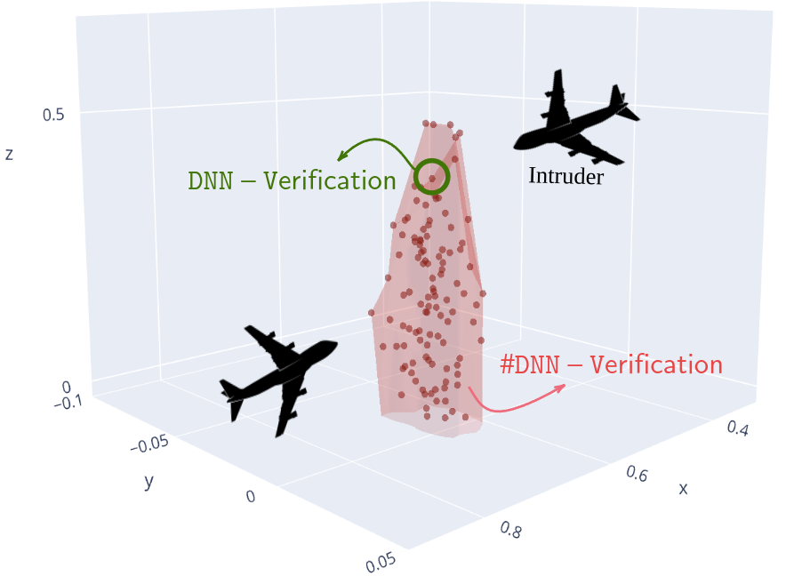
Figure 3: Explanatory image of the possible impact of #DNN-Verification in safety-critical contexts. A standard verifier returns only a violation point (highlighted in the image with a green circle), limiting the interpretability of the results. In contrast, our approach paves the way to estimate the entire dangerous area (depicted in red in the figure).

Experiments on a Different Property

To validate the correctness of our approximation, we also performed a final experiment on property $\phi_{3}$ of the Acas Xu benchmark. In particular, this property encodes a scenario in which if the intruder is directly ahead and is moving towards the ownship, the score for COC will not be minimal (we refer to Katz et al. [2017] for further details). This property is particularly interesting as it holds for all 45 models, i.e., we expect a 0% of violation rate for each model tested. For simplicity, in Tab. 7 we report only the first 5 models since the results were very similar for all the DNNs tested. As expected, we empirically confirmed that also for this particular situation, the lower and upper bounds computed with CountingProVe never overestimate and underestimate respectively the true value of the violation rate, in this case, 0%.

Instance	CountingProVe (confidence $\geq$ 99%)
	Interval confidence VR	Size	Time
$\phi_{3}$ ACAS Xu_1.1	[0%, 2.26%]	2.26%	215 min
$\phi_{3}$ ACAS Xu_1.2	[0%, 2.88%]	2.88%	216 min
$\phi_{3}$ ACAS Xu_1.3	[0%, 2.30%]	2.30%	215 min
$\phi_{3}$ ACAS Xu_1.4	[0%, 2.47%]	2.47%	218 min
$\phi_{3}$ ACAS Xu_1.5	[0%, 2.48%]	2.48%	214 min

Table 7: CountingProVe on ACAS Xu $\phi_{3}$ property

Instance		Exact Count		CountingProVe (confidence $\geq 99\%$)
		BaB
		Violation Rate	Time	Interval confidence VR	Size	Time
$\phi_{2}$ ACAS Xu_2.1		–	24 hrs	[0.45%, 5.01%]	4.56%	246 min
$\phi_{2}$ ACAS Xu_2.2		–	24 hrs	[1.06%, 4.81%]	3.75%	246 min
$\phi_{2}$ ACAS Xu_2.3		–	24 hrs	[1.23%, 4.21%]	2.98%	241 min
$\phi_{2}$ ACAS Xu_2.4		–	24 hrs	[0.74%, 3.43%]	2.68%	243 min
$\phi_{2}$ ACAS Xu_2.5		–	24 hrs	[1.67%, 4.10%]	2.42%	240 min
$\phi_{2}$ ACAS Xu_2.6		–	24 hrs	[1.01%, 3.59%]	2.58%	248 min
$\phi_{2}$ ACAS Xu_2.7		–	24 hrs	[2.35%, 5.22%]	2.87%	240 min
$\phi_{2}$ ACAS Xu_2.8		–	24 hrs	[1.77%, 4.68%]	2.92%	248 min
$\phi_{2}$ ACAS Xu_2.9		–	24 hrs	[0.18%, 2.77%]	2.59%	239 min
$\phi_{2}$ ACAS Xu_3.1		–	24 hrs	[1.62%, 4.98%]	3.36%	242 min
$\phi_{2}$ ACAS Xu_3.2		–	24 hrs	[0%, 2.50%]	2.5%	243 min
$\phi_{2}$ ACAS Xu_3.3		–	24 hrs	[0%, 2.54%]	2.54%	245 min
$\phi_{2}$ ACAS Xu_3.4		–	24 hrs	[0.26%, 3.08%]	2.82%	244 min
$\phi_{2}$ ACAS Xu_3.5		–	24 hrs	[0.92%, 3.60%]	2.68%	244 min
$\phi_{2}$ ACAS Xu_3.6		–	24 hrs	[1.71%, 4.48%]	2.77%	251 min
$\phi_{2}$ ACAS Xu_3.7		–	24 hrs	[0.14%, 2.64%]	2.49%	213 min
$\phi_{2}$ ACAS Xu_3.8		–	24 hrs	[0.75%, 3.28%]	2.54%	216 min
$\phi_{2}$ ACAS Xu_3.9		–	24 hrs	[2.11%, 5.20%]	3.09%	242 min
$\phi_{2}$ ACAS Xu_4.1		–	24 hrs	[0.33%, 3.04%]	2.71%	246 min
$\phi_{2}$ ACAS Xu_4.3		–	24 hrs	[1.3%, 3.61%]	2.31%	243 min
$\phi_{2}$ ACAS Xu_4.4		–	24 hrs	[0.79%, 3.57%]	2.79%	247 min
$\phi_{2}$ ACAS Xu_4.5		–	24 hrs	[0.71%, 4.03%]	3.33%	240 min
$\phi_{2}$ ACAS Xu_4.6		–	24 hrs	[1.65%, 4.72%]	3.08%	244 min
$\phi_{2}$ ACAS Xu_4.7		–	24 hrs	[1.67%, 4.33%]	2.66%	248 min
$\phi_{2}$ ACAS Xu_4.8		–	24 hrs	[1.68%, 4.17%]	2.49%	241 min
$\phi_{2}$ ACAS Xu_4.9		–	24 hrs	[0.10%, 2.61%]	2.51%	247 min
$\phi_{2}$ ACAS Xu_5.1		–	24 hrs	[1.06%, 3.76%]	2.7%	240 min
$\phi_{2}$ ACAS Xu_5.2		–	24 hrs	[0.86%, 3.58%]	2.72%	248 min
$\phi_{2}$ ACAS Xu_5.4		–	24 hrs	[0.75%, 3.25%]	2.5%	239 min
$\phi_{2}$ ACAS Xu_5.5		–	24 hrs	[1.66%, 4.35%]	2.68%	247 min
$\phi_{2}$ ACAS Xu_5.6		–	24 hrs	[1.81%, 4.45%]	2.64%	240 min
$\phi_{2}$ ACAS Xu_5.7		–	24 hrs	[1.75%, 5.15%]	3.40%	246 min
$\phi_{2}$ ACAS Xu_5.8		–	24 hrs	[1.96%, 4.65%]	2.70%	241 min
$\phi_{2}$ ACAS Xu_5.9		–	24 hrs	[1.62%, 4.40%]	2.77%	241 min
				Mean	2.83%	242 min

Table 8: Comparison of CountingProVe and exact counters on different benchmark setups.

References

- Amir et al. [2023] Guy Amir, Davide Corsi, Raz Yerushalmi, Luca Marzari, David Harel, Alessandro Farinelli, and Guy Katz. Verifying learning-based robotic navigation systems. In 29th International Conference, TACAS 2023, pages 607–627. Springer, 2023.
- Baluta et al. [2019] Teodora Baluta, Shiqi Shen, Shweta Shinde, Kuldeep S. Meel, and Prateek Saxena. Quantitative verification of neural networks and its security applications. In Proceedings of the 2019 ACM SIGSAC Conference on Computer and Communications Security, 2019.
- Bunel et al. [2018] Rudy R Bunel, Ilker Turkaslan, Philip Torr, Pushmeet Kohli, and Pawan K Mudigonda. A unified view of piecewise linear neural network verification. Advances in Neural Information Processing Systems, 31, 2018.
- Corsi et al. [2021] Davide Corsi, Enrico Marchesini, and Alessandro Farinelli. Formal verification of neural networks for safety-critical tasks in deep reinforcement learning. In Uncertainty in Artificial Intelligence, pages 333–343. PMLR, 2021.
- Ghosh et al. [2021] Bishwamittra Ghosh, Debabrota Basu, and Kuldeep S Meel. Justicia: A stochastic sat approach to formally verify fairness. In Proceedings of the AAAI Conference on Artificial Intelligence, pages 7554–7563, 2021.
- Gomes et al. [2007] Carla P Gomes, Jörg Hoffmann, Ashish Sabharwal, and Bart Selman. From sampling to model counting. In IJCAI, volume 2007, pages 2293–2299, 2007.
- Gomes et al. [2021] Carla P Gomes, Ashish Sabharwal, and Bart Selman. Model counting. In Handbook of satisfiability, pages 993–1014. IOS press, 2021.
- Katz et al. [2017] Guy Katz, Clark Barrett, David L Dill, Kyle Julian, and Mykel J Kochenderfer. Reluplex: An efficient smt solver for verifying deep neural networks. In International conference on computer aided verification, pages 97–117. Springer, 2017.
- Katz et al. [2019] Guy Katz, Derek A Huang, Duligur Ibeling, Kyle Julian, Christopher Lazarus, Rachel Lim, Parth Shah, Shantanu Thakoor, Haoze Wu, Aleksandar Zeljić, et al. The marabou framework for verification and analysis of deep neural networks. In International Conference on Computer Aided Verification, 2019.
- Katz et al. [2021] Guy Katz, Clark Barrett, David L Dill, Kyle Julian, and Mykel J Kochenderfer. Reluplex: a calculus for reasoning about deep neural networks. Formal Methods in System Design, pages 1–30, 2021.
- Liu et al. [2021] Changliu Liu, Tomer Arnon, Christopher Lazarus, Christopher Strong, Clark Barrett, Mykel J Kochenderfer, et al. Algorithms for verifying deep neural networks. Foundations and Trends® in Optimization, 4(3-4):244–404, 2021.
- Lomuscio and Maganti [2017] Alessio Lomuscio and Lalit Maganti. An approach to reachability analysis for feed-forward relu neural networks. arXiv preprint arXiv:1706.07351, 2017.
- Marchesini et al. [2021] Enrico Marchesini, Davide Corsi, and Alessandro Farinelli. Benchmarking safe deep reinforcement learning in aquatic navigation. In 2021 IEEE/RSJ International Conference on Intelligent Robots and Systems (IROS), pages 5590–5595, 2021.
- Marchesini et al. [2022] Enrico Marchesini, Davide Corsi, and Alessandro Farinelli. Exploring safer behaviors for deep reinforcement learning. In Association for the Advancement of Artificial Intelligence (AAAI), 2022.
- Marzari et al. [2022] Luca Marzari, Davide Corsi, Enrico Marchesini, and Alessandro Farinelli. Curriculum learning for safe mapless navigation. In Proceedings of the 37th ACM/SIGAPP Symposium on Applied Computing, pages 766–769, 2022.
- Marzari et al. [2023] Luca Marzari, Enrico Marchesini, and Alessandro Farinelli. Online safety property collection and refinement for safe deep reinforcement learning in mapless navigation. In 2023 IEEE International Conference on Robotics and Automation (ICRA). IEEE, 2023.
- Moore et al. [2009] Ramon E Moore, R Baker Kearfott, and Michael J Cloud. Introduction to interval analysis. SIAM, 2009.
- Szegedy et al. [2013] Christian Szegedy, Wojciech Zaremba, Ilya Sutskever, Joan Bruna, Dumitru Erhan, Ian Goodfellow, and Rob Fergus. Intriguing properties of neural networks. arXiv preprint arXiv:1312.6199, 2013.
- Tjeng et al. [2018] Vincent Tjeng, Kai Y Xiao, and Russ Tedrake. Evaluating robustness of neural networks with mixed integer programming. In International Conference on Learning Representations, 2018.
- Valiant [1979] Leslie G Valiant. The complexity of enumeration and reliability problems. SIAM Journal on Computing, 8(3):410–421, 1979.
- Wang et al. [2018] Shiqi Wang, Kexin Pei, Justin Whitehouse, Junfeng Yang, and Suman Jana. Efficient formal safety analysis of neural networks. Advances in Neural Information Processing Systems, 31, 2018.
- Wang et al. [2021] Shiqi Wang, Huan Zhang, Kaidi Xu, Xue Lin, Suman Jana, Cho-Jui Hsieh, and J Zico Kolter. Beta-crown: Efficient bound propagation with per-neuron split constraints for neural network robustness verification. Advances in Neural Information Processing Systems, 34:29909–29921, 2021.
- Zhang et al. [2021] Yedi Zhang, Zhe Zhao, Guangke Chen, Fu Song, and Taolue Chen. Bdd4bnn: a bdd-based quantitative analysis framework for binarized neural networks. In Computer Aided Verification: 33rd International Conference, CAV 2021, Virtual Event, July 20–23, 2021, Proceedings, Part I 33, pages 175–200. Springer, 2021.