Solving various NP-Hard problems using exponentially fewer qubits
on a Quantum Computer

Abstract

NP-hard problems are not believed to be exactly solvable through general polynomial time algorithms. Hybrid quantum-classical algorithms to address such combinatorial problems have been of great interest in the past few years. Such algorithms are heuristic in nature and aim to obtain an approximate solution. Significant improvements in computational time and/or the ability to treat large problems are some of the principal promises of quantum computing in this regard. The hardware, however, is still in its infancy and the current Noisy Intermediate Scale Quantum (NISQ) computers are not able to optimize industrially relevant problems. Moreover, the storage of qubits and introduction of entanglement require extreme physical conditions. An issue with quantum optimization algorithms such as QAOA is that they scale linearly with problem size. In this paper, we build upon a proprietary methodology which scales logarithmically with problem size – opening an avenue for treating optimization problems of unprecedented scale on gate-based quantum computers. In order to test the performance of the algorithm, we first find a way to apply it to a handful of NP-hard problems: Maximum Cut, Minimum Partition, Maximum Clique, Maximum Weighted Independent Set. Subsequently, these algorithms are tested on a quantum simulator with graph sizes of over a hundred nodes and on a real quantum computer up to graph sizes of 256. To our knowledge, these constitute the largest realistic combinatorial optimization problems ever run on a NISQ device, overcoming previous problem sizes by almost tenfold.

I Introduction

NP-hard problems are problems that do not have algorithms that can give an exact solution in polynomial time, whereas it is ’easy’ to verify the solution if it is known [1, 2, 3]. While finding exact solutions to large problems is difficult, there exist many algorithms that find approximate solutions to these problems [4, 5, 6, 7]. In the scope of quantum computing, a huge amount of research has been carried out on hybrid quantum-classical algorithms [8, 9, 10, 11, 12, 13, 14, 15, 16, 17, 18, 19, 20]. In such algorithms, quantum circuit measurements are used in tandem with a classical optimization loop to obtain an approximate solution.

One of the most commonly used hybrid algorithms is the Quantum Approximate Optimization Algorithm (QAOA) [8, 21, 22, 23, 24]. One of the main drawbacks of the QAOA is that the number of qubits required scales linearly with problem size [25]. This means that a graph of $n$ nodes would require an $n$-qubit quantum computer to be solved. At the moment, the largest available universal gate-based quantum computer is IBM’s Osprey device, containing 433 qubits. All the qubits are not of the same quality and the larger the problem, the more likely it is to obtain noisier results due to the presence of qubits with higher error rates. Moreover, these qubits are not all-in-all connected, meaning that in case of large sized problem, numerous SWAP gates would have to be used in order to run the circuit, leading to more noise.

It is therefore not surprising that a smaller scale quantum computer is likely to provide much better results that a larger one. In light of this, an algorithm to encode the Maximum Cut problem on a quantum computer using logarithmically fewer qubits was developed [26]. This encoding allows us to represent much larger problems using a fairly small number of qubits. Therefore a Maximum Cut problem with a graph of $n$ nodes can be represented using only $\lceil\log_{2}n\rceil$ qubits.

Since the developed algorithm deals specifically with solving the Maximum Cut problem, a logical extension of this algorithm would be to expand the applicability of the algorithm to other problems. This can be approached in two ways, as shall be demonstrated in the following sections.

The paper is structured as follows. In section II.2, we describe in detail the logarithmic encoding of the Maximum Cut problem on a quantum computer. In section II.3, we show how this algorithm can be applied on a variety of NP-hard problems by converting them, directly or indirectly, to the Maximum Cut problem. In section II.4, we show how any Quadratic Unconstrained Binary Optimization Problem (QUBO) problem can be treated using the logarithmic encoding. In section III, experimental results of all the methods described in the previous sections are shown. Notably, we show quantum simulator results with instances of sizes of over a hundred nodes/objects, as well as quantum hardware (QPU) results for problem sizes up to 256.

II Methods

II.1 An Introduction to the Quantum Model of Computation

Quantum computing [27, 28, 29, 30] presents a new way of doing computations by making use of fundamental properties of quantum mechanics such as superposition and entanglement. A classical bit consists of 2 possible states, $0$ and $1$. In quantum computing the first building block is the quantum bit or qubit. Much like a classical bit, a qubit has 2 basis states $\ket{0}$ and $\ket{1}$.

However unlike a classical bit, a qubit can exist in any linear combination of $\ket{0}$ and $\ket{1}$. Let $\ket{\psi}$ define the state of a qubit, then it can be mathematically defined as:

$$\ket{\psi}=\alpha\ket{0}+\beta\ket{1}$$ (1)

where $\alpha$ and $\beta$ are complex coefficients such that $|\alpha|^{2}+|\beta|^{2}=1$. The coefficients $\alpha$ and $\beta$ are such that $|\alpha|^{2}$ and $|\beta|^{2}$ represent the probability of a qubit being in the state $\ket{0}$ and $\ket{1}$ respectively. The existence of qubits in all the intermediate states between $0$ and $1$ is called superposition.

Another important concept is that of entanglement. Two qubits are said to be entangled if they cannot be represented as a product state. This means that they can only be written in a combined superposition of all possible two-qubit basis states. Let $\ket{\Psi}$ be an $N$-qubit state. It can be represented mathematically as follows:

$$\ket{\Psi}=\sum\limits_{i\in\{0,1\}^{N}}c_{i}\ket{i}$$ (2)

To completely describe the $N$-qubit state, we will require $2^{N}$ coefficients. If there is no entanglement then each qubit can be expressed separately. From equation (1) it can be seen that we need 2 coefficients to encode a single qubit and therefore we would need only $2N$ coefficients to represent $N$ non-entangled qubits. Entanglement is therefore of paramount importance in quantum computing as it helps encode much more information.

The specific model of quantum computation used in this paper is called gate-based quantum computing. There exist other types of quantum computing such as quantum annealing [31], topological quantum computing [32] and measurement-based quantum computing [33]. They are, however, beyond the scope of this paper. In the gate-based model we create a quantum circuit which is a combination of qubits and operations on qubits.

Operations on qubits are known as quantum gates. Mathematically, these can be represented by square matrices. A important property of gates is that they must be Hermitian. There are 2 basic types of gates:

1. Single qubit gates : They act on a single qubit and alter the state of the qubit.

2. Multiple qubit gates : These gates act on multiple qubits. These are also referred to as entangling gates. The simplest entangling gate is the CNOT gate.

All quantum operations can be represented using single qubit gates and the CNOT gate. The gate-based model is therefore a universal model of quantum computation.

Once we have created a circuit out of qubits and gates we finally need to ’measure’ our qubits, which is equivalent to calculating the expectation value the system. Let all the gates in the circuit be represented by unitary matrix $U$. If it is applied to the initial state $\ket{\Psi}$, we have the following final state:

$$\ket{\Psi^{\prime}}=U\ket{\Psi}$$ (3)

The expectation value of a measurable $H$ is given by the following expression:

$$\braket{H}=\bra{\Psi^{\prime}}H\ket{\Psi^{\prime}}$$ (4)

A measurable can be mathematically represented by a Hermitian matrix.

Since quantum computers were first theorized in the 1980s, theoretical advantages of quantum algorithms compared to their classical counterparts have been proven for several problems [34, 35, 36]. However, implementing them requires a significant amount of high quality quantum resources. Specifically, they need quantum computers with many qubits as well as the ability to handle a lot of quantum operations (gates) without generating much noise. In other words, they should be able to run deep quantum circuits on several qubits. Such quantum computers might become available in the medium term but at present we have noisy intermediate-scale quantum (NISQ) computers, which cannot handle these algorithms. This has led to a significant amount of research in the development of hybrid algorithms that can run on currently available hardware.

II.2 A qubit-efficient Maximum Cut Algorithm

Contemporary quantum optimization algorithms in general scale linearly with problem size. This means that if the problem consists of an $n$ node graph, the algorithm will require $n$ qubits to solve the problem. Note that to solve a problem here implies to obtain an approximate solution. Following Ref. [26], we present an algorithm that scales logarithmically with the problem size. For a problem of size $n$, the number of qubits required is $\lceil\log_{2}n\rceil$.

II.2.1 Description of the algorithm

Recall first the definition of Maximum Cut:

Maximum Cut Input A weighted graph $G(V,E,w)$. Task Find $x\in\{1,-1\}^{|V|}$ that maximizes $\sum_{ij}w_{ij}\dfrac{(1-x_{i})(1+x_{j})}{4}\forall\{(i,j)\in E\}$, where $w_{ij}$ are the weights on the edges.

Given a graph $G(V,E)$, the Maximum Cut can be represented using the graph Laplacian matrix. The graph Laplacian is defined as follows:

$$L_{ij}=\begin{cases}degree(i)\quad&\text{if }\,i=j\\ -w_{ij}\quad&\text{if }\,i\neq j\text{ and }(i,j)\in E\\ 0\quad&\text{otherwise}\end{cases}$$ (5)

Note that the degree here is a weighted degree.

The Maximum Cut value is given by the following equation [37]:

$$\text{{Maximum Cut}}=\frac{1}{4}x^{T}Lx$$ (6)

where $L$ is the Laplacian matrix and $x\in\{1,-1\}^{|V|}$ is the bi-partition vector.

Due to fact that the Laplacian is a Hermitian matrix, it resembles a Hamiltonian of an actual physical system. The quantum analog of equation (6) is

$$C(\theta_{1}...\theta_{n})=2^{n-2}\bra{\Psi(\theta_{1}...\theta_{n})}L\ket{\Psi(\theta_{1}...\theta_{n})}$$ (7)

where $L$ is the Laplacian matrix of the graph, $\ket{\Psi}$ is the parameterized ansatz, $n$ is the size of the graph, and $\theta=\{\theta_{1}....\theta_{n}\}$ are the variables to be optimized. $2^{n-2}$ is the normalization constant.

As described in Figure 1, we have designed a variational algorithm that finds a good approximation to the best Maximum Cut. Starting from the initial values of $\theta$ parameters, we call a quantum circuit to evaluate the objective function (Algorithm 1) and run a classical black box optimization loop over the $\theta$ parameters (Algorithm 2). As a result, we obtain $\theta^{*}$ to evaluate the best solution.

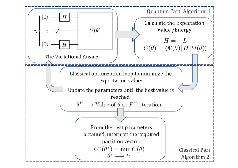
Figure 1: Diagrammatic representation of the hybrid quantum-classical algorithm.

To evaluate the expectation value $C$ on a quantum computer, first we need to create the ansatz $\ket{\Psi(\theta_{1}...\theta_{n})}$. In order to do this the following steps are required.

1. We define a function $R(\theta_{k})$ as follows:

   $$R(\theta_{k})=\begin{cases}0\quad&\text{if }\,0\leq\theta_{k}<\pi\\ 1\quad&\text{if }\,\pi\leq\theta_{k}<2\pi\\ \end{cases}$$ (8)

   Therefore,

   $$\exp(i\pi R(\theta_{k}))=\begin{cases}1\quad&\text{if }\,0\leq\theta_{k}<\pi\\ -1\quad&\text{if }\,\pi\leq\theta_{k}<2\pi\\ \end{cases}$$ (9)

   The point of doing this is that not all classical optimizers accept binary variables. The function $R$ converts a continuous variable into a binary one, which is what we need.

2. Given a graph $G(V,E)$ such that $|V|=n$ and $|E|=m$, to create the ansatz we first define the number of qubits required as follows:

   $$N=\lceil\log_{2}n\rceil$$ (10)

   When the number of nodes are not an exact power of 2, we can adjust $L$ to be of size $2^{N}$ by adding null matrices of size $2^{N}-|V|$, $\mathbb{O}_{2^{N}-|V|}$, as shown in line 3, Algorithm 1.

3. Create a quantum circuit and apply a Hadamard gate to all the qubits to achieve an equal superposition of the states (lines 7 and 8, Algorithm 1).

4. To the circuit, apply a diagonal gate $U$ (line 9, Algorithm 1) of the following form:

   $$U(\theta)=\begin{bmatrix}e^{i\pi R(\theta_{1})}&0&0&....\\ 0&e^{i\pi R(\theta_{2})}&0&....\\ ....&....&....&....\\ 0&0&0&e^{i\pi R(\theta_{n})}\end{bmatrix}$$ (11)

   Therefore the final ansatz is:

   $$\ket{\Psi(\theta)}=U(\theta)H^{\otimes N}\ket{0}^{\otimes N}$$ (12)

   The state in the above equation is obtained in line 10 of Algorithm 1.

Having an ansatz, we can now define the Laplacian as an observable and evaluate the measurement (as in equation 7) which is the energy of the system. Since the classical optimizer minimizes the cost function we take the negative of the Laplacian matrix. Thus the final cost function is:

$$C(\theta)=-2^{n-2}\bra{\Psi(\theta)}L\ket{\Psi(\theta)}$$ (13)

To evaluate this expectation value, the Laplacian matrix needs to be converted into a sum of tensor products of Pauli matrices (line 4 Algorithm 1, see Appendix A).

Using classical black-box meta optimizers such as COBYLA, Nelder-Mead or Genetic Algorithm (as detailed in Algorithm 2), we then obtain

$$C^{*}(\theta^{*})=\min C(\theta)$$ (14)

The final parameters obtained $\theta^{*}$ gives the bi-partition vector, using equation (9).

Input: Laplacian matrix of a graph $G(V,E)$

1 $L\leftarrow$Graph Laplacian of size $|V|\times|V|$

2 $N\leftarrow\lceil\log_{2}|V|\rceil$

3 $L^{*}\leftarrow\begin{bmatrix}L&\mathbb{O}_{2^{N}-|V|}\\ \mathbb{O}_{2^{N}-|V|}&\mathbb{O}_{2^{N}-|V|}\end{bmatrix}$

4 $H\leftarrow\dfrac{1}{n}\sum\limits_{i=1}^{4^{N}}Tr(J_{i}\cdot L^{*})J_{i}\text{ where }J=\{\prod_{k=1}^{N}S^{\otimes k}\}$

5 $\theta\leftarrow$ List of $|V|$ parameters

6

7Function EvalCost($\theta$ ):

8       $Q\leftarrow$ Quantum Circuit of $N$ qubits

9       Add Hadamard gate to each Qubit

10       $U\leftarrow$ diagonal gate $diag(\theta,R)$

11       Apply $U$ to $Q$

12       $F\leftarrow ExpectationValue(Q,H)$

13       return $2^{|V|-2}F$

14      

15

16

17

Algorithm 1 Log Encoding of Maximum Cut: Building the Objective Function

Input: EvalCost($\theta$)

1

2Function Optimizer(EvalCost($\theta$),$\theta^{\text{initial}}$ ):

3      

4      repeat

5             $\theta^{p}\leftarrow\theta\text{ at }p^{th}\text{ iteration}$

6             $C\leftarrow$ EvalCost($\theta^{p}$)

7             if C is sufficiently good then

8                  $C^{*}\leftarrow C$

9                  break

10            else

11                  Update $\theta^{p}\rightarrow\theta^{p+1}$

12                  continue

13             end if

14            

15      

16      

17      return $C^{*}$

18      

19

20

21

Algorithm 2 Log Encoding of Maximum Cut: Minimizing the Objective Function

II.2.2 Advantages and disadvantages of the algorithm

The algorithm helps us represent large problems (by current standards of quantum computing) on a quantum computer. Algorithms like the QAOA, for example, require 128 qubits to represent a 128-node Maximum Cut problem. The same problem can be solved by the proposed algorithm using only 7 qubits. A problem with over a million nodes can be represented with just 20 qubits, something that is quite unthinkable using contemporary algorithms. It therefore has the promise of being able to be applied to interesting and even industrially relevant sizes using the currently available sizes of NISQ QCs. While the QAOA depends on the availability of a large number of qubits for the algorithm to work on any interesting problem, the above algorithm only depends on an increased accuracy in QCs of current size. The number of CNOT gates required for the QAOA ansatz is $p|E|$, where $p$ is the depth of the algorithm (for all practical purposes, $p\gg 1$ [38]) and $|E|$ is the number of edges in the graph. In our algorithm the number of CNOTs is equal to $|V|-1$, $|V|$ being the number of vertices. Generally, and especially at higher densities, it is easy to see that $p|E|\gg|V|$. This means that our circuit turns out to be much shallower than that of QAOA.

In our study, the search space remains the same as that of the classical search space. A procedure to reduce the number of variables has been presented in [26]. However, this method is beyond the scope of the current work. Readers should also refer to followup studies [39] where the algorithm was evaluated on the Maximum Cut problem by using the alternating optimization procedure [40] which scales polynomially in problem size.

II.3 Applying the algorithm to other NP-hard problems

A logical next step is to attempt to solve a variety of combinatorial optimisation problems using the algorithm. In Karp’s paper from 1972 [41], he outlined how we can convert one NP-complete problem into another. A more recent paper [42] lists numerous more such reductions. Figure 2 shows a subset (a transformation family) of these reductions directly or indirectly relating to Maximum Cut. Here, we follow a similar logic to convert various NP-hard problems to Maximum Cut.

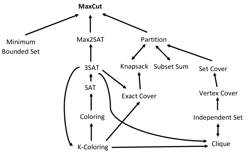
Figure 2: Graph of Maximum Cut transformation family for NP-complete problems.

Note, however, that these conversions might not have a one-to-one scaling. For example, an $n$ variable Maximum 2-Sat problem requires us to solve a $2n$ node Maximum Cut problem.

In Karp’s paper all the transitions are from one decision problem to another. Usually in classical computing it would be considered trivial to convert a decision problem into an optimisation one. However, our algorithm is inherently an optimisation algorithm and moreover will give various results for a various runs. The point being, it will not respond well to yes-no decision problems. Therefore, it is important to make reductions between the optimisation versions. Moreover it is important to make sure that these conversions support a wide definition of the problems (for example Maximum 3-Sat instead of 3-Sat).

Following are some such polynomial-time reductions of NP-hard problems:

II.3.1 Minimum Partition to Maximum Cut

Minimum Partition Input A set $S=\{w:w\in\mathbb{Z}^{+}\}$. Task Find $A\subseteq S$ that minimizes
$|\sum\limits_{w_{k}\in A}{w_{k}}-\sum\limits_{w_{l}\notin A}{w_{l}}|$.

This can be converted to the maximum cut problem in the following manner:

1. Create a graph such that there is a node for every number.

2. For every pair of nodes $(i,j)$, connect them using an edge of weight $w_{i}*w_{j}$.

3. The maximum cut value of this graph gives a bi-partition that is equivalent to the minimum partition.

II.3.2 Maximum 2-Sat to Maximum Cut

Maximum 2-Sat Input A set of $m$ clauses $C=\{w_{pq}(x_{p}+x_{q}):x_{p},x_{q}\in X\cup X^{\prime}\}$ where $X=\{x:x\in\{0,1\}\}$, $X^{\prime}=\{\overline{x}:x\in X\}$ and $w_{pq}$ are the clause weights. Task Find the variable assignment $X$ that maximizes the combined weight of the satisfied clauses.

The problem is said to be satisfiable if all the clauses are satisfied.

We can convert this problem into the maximum cut problem in the following manner:

1. In a graph, assign 2 nodes for every variable, one for the variable and another for the complement of the variable. Hence there are $2|X|$ nodes in the graph.

2. Draw an edge between the nodes representing the variables and their complements. For example connect $x_{1}$ and $\overline{x_{1}}$, $x_{2}$ and $\overline{x_{2}}$ and so on. Add a large edge weight (about $10^{m}$). This is to make sure that the variables and their complements do not fall in the same partition.

3. For every clause, add an edge between the respective nodes with edge weight as $w_{pq}$.

4. The maximum cut of this graph is equivalent to the Maximum 2-Sat solution.

II.3.3 Maximum Clique to Maximum 2-Sat

Maximum Clique Input A graph $G(V,E)$. Task Maximize $|V^{\prime}|$ in the graph $\{G^{\prime}(V^{\prime},E^{\prime}):V^{\prime}\subseteq V,E^{\prime}\subseteq E,|E^{\prime}|=\frac{|V^{\prime}|(|V^{\prime}|-1)}{2}\}$.

It can be converted to the Maximum 2-Sat problem in the following manner:

1. Consider a graph $G(V,E)$ having vertices $v_{i}\in V$. For each vertex $v_{i}$ add a variable $x_{i}$. Also an auxiliary variable $z$. We therefore have $|V|+1$ variables.

2. For every variable add the following 2 clauses: $(x_{i}+z)$ and $(x_{i}+\overline{z})$. Let us refer to these clauses as Type A clauses.

3. Add the following clauses: $(\overline{x_{i}}+\overline{x_{j}})\text{ }\forall\text{ }(i,j)\notin E$. We will refer to these clauses as clauses of type B.

4. The clauses of type A ensure that the maximum number of nodes are selected and the clauses of type B make sure that the selected subgraph is a clique.

5. To the type B clauses, add a large weight. Due to the nature of the algorithm and it’s susceptibility to errors, we may get solutions that are not cliques at all. Moreover finding a clique and maximizing it are 2 different problems and by adding weights we make sure that they are not affected by one another.

6. The Maximum 2-Sat problem is solved for this set of clauses. The partition of selected variables form the Maximum Clique.

II.4 Generalizing the Algorithm

The algorithm described above solves, originally, the Maximum Cut problem. Various conversions are then used in order to solve other problems. Here, a second, more general approach, shall be described, where any problem which can be written in the form of a Quadratic Unconstrained Binary Optimization (QUBO) problem [43] can be solved. Instead of taking the Laplacian matrix as the input, this algorithm takes as input the QUBO matrix of the problem.

Firstly, we define the QUBO matrix. To describe a problem as a QUBO, all the terms in the objective function should be either linear or quadratic. Since the variables in the objective function are binary, a linear term can be easily converted to a quadratic one, since $x_{i}^{2}=x_{i}\text{ }\forall\text{ }x\in\{0,1\}$.

Consider the objective function of the following form:

$$P=\sum_{\begin{subarray}{c}ij\end{subarray}}a_{ij}x_{i}x_{j}$$ (15)

It can be rewritten as:

$$P=\begin{pmatrix}x_{1}&x_{2}&...&x_{n}\end{pmatrix}\begin{pmatrix}a_{11}&a_{12}&...&a_{1n}\\ a_{21}&a_{22}&...&a_{2n}\\ ...&...&...&...\\ a_{n1}&a_{n2}&...&a_{nn}\end{pmatrix}\begin{pmatrix}x_{1}\\ x_{2}\\ ...\\ x_{n}\end{pmatrix}$$ (16)

$$P=x^{T}Qx$$ (17)

$$Q=\begin{pmatrix}a_{11}&a_{12}&...&a_{1n}\\ a_{21}&a_{22}&...&a_{2n}\\ ...&...&...&...\\ a_{n1}&a_{n2}&...&a_{nn}\end{pmatrix}$$ (18)

$Q$ is the required QUBO matrix.

This matrix cannot be directly used in the algorithm. This is because in the original Maximum Cut algorithm, the variable used belongs to the set $\{1,-1\}$ and not $\{0,1\}$. To make the equation mathematically consistent, we need to reformulate the QUBO matrix.

Let $z\in\{1,-1\}$ and $x\in\{0,1\}$, then $x=\dfrac{1-z}{2}$. Equation (15) therefore becomes:

$$P=\sum_{i}a_{ii}\dfrac{1-z_{i}}{2}+\sum_{\begin{subarray}{c}ij\\ i\neq j\end{subarray}}a_{ij}\dfrac{1-z_{i}}{2}\dfrac{1-z_{j}}{2}$$ (19)

Note that in the first term $\dfrac{1-z_{i}}{2}$ has been used instead of $\bigg{(}\dfrac{1-z_{i}}{2}\bigg{)}^{2}$ since $x_{i}^{2}=x_{i}$.

In the search for optimal values of parameters $z$ we can eliminate the constant terms in $P$ as they only add a constant shift to the cost function. We can therefore simplify (19) as follows:

$$P =\sum_{i}a_{ii}\dfrac{1-z_{i}}{2}+\sum_{\begin{subarray}{c}ij\\ i\neq j\end{subarray}}a_{ij}\dfrac{1-z_{i}}{2}\dfrac{1-z_{j}}{2}$$ (20)

$$=\dfrac{1}{2}\sum_{i}a_{ii}(1-z_{i})+\dfrac{1}{4}\sum_{\begin{subarray}{c}ij\\ i\neq j\end{subarray}}a_{ij}(1-z_{i}-z_{j}+z_{i}z_{j})$$ (21)

$$=-\dfrac{1}{2}\sum_{i}a_{ii}z_{i}+\dfrac{1}{4}\sum_{\begin{subarray}{c}ij\\ i\neq j\end{subarray}}a_{ij}(-z_{i}-z_{j}+z_{i}z_{j})$$ (22)

The above cannot be represented in a matrix form similar to Eq. 18 since it has linear terms that cannot be quadratized since $z_{i}^{2}\neq z_{i}$.

We therefore need to reformulate the problem. In this reformulation the linear terms are represented in the off-diagonal terms instead of the diagonals. Let us have $2n$ variables $\{z_{1},z_{2}....z_{2n}\}$ where $z_{1}...z_{n}\in\{1,-1\}$ and $z_{n+1}...z_{2n}\in\{1\}$. Then to represent a linear variable $z_{i}$, we can have the term $z_{i}z_{i+n}$ where $z_{i+n}=1$. The equation (22) can be rewritten as follows:

$$P=-\dfrac{1}{2}\sum_{i}a_{ii}z_{i}z_{i+n}+\dfrac{1}{4}\sum_{\begin{subarray}{c}ij\\ i\neq j\end{subarray}}a_{ij}(-z_{i}z_{i+n}-z_{j}z_{j+n}+z_{i}z_{j})$$ (23)

This is our reformulated QUBO, which we shall call the spin-QUBO(sQUBO). This is a matrix of size $2n\times 2n$. It will require $\lceil\log_{2}2n\rceil=(1+\lceil\log_{2}n\rceil$) qubits, or, in other words, 1 more qubit than the original algorithm. Note that this is still an optimization problem of $n$ variables since the variables $z_{n+1}...z_{2n}$ are fixed.

Using our formulation, we propose that any problem that can be represented in a QUBO format can be solved using the algorithm described in Algorithm 3.

Input: QUBO Matrix

1 Convert $QUBO$ to $sQUBO$

2 $Q\leftarrow$sQUBO

3 $N\leftarrow\lceil\log_{2}2n\rceil$

4 $Q^{*}\leftarrow\begin{bmatrix}Q&\mathbb{O}_{2^{N}-n}\\ \mathbb{O}_{2^{N}-n}&\mathbb{O}_{2^{N}-n}\end{bmatrix}$

5 $H\leftarrow\dfrac{1}{n}\sum\limits_{i=1}^{4^{N}}Tr(J_{i}\cdot Q^{*})J_{i}\text{ where }J=\{\prod_{k=1}^{N}S^{\otimes k}\}$

6 $\theta\leftarrow$ List of $n$ parameters

7

8Function EvalCost($\theta$ ):

9       $QC\leftarrow$ Quantum Circuit of N qubits

10       Add Hadamard gate to each Qubit

11       $U\leftarrow$ diagonal gate $diag(\theta,R)$

12       Apply $U$ to $QC$

13       $F\leftarrow ExpectationValue(Q,H)$

14       return $F$

15      

16

17

18

Algorithm 3 Log Encoding of a QUBO problem: Building the Objective Function

II.4.1 Maximum Weighted Independent Set using QUBO

Maximum Weighted Independent Set Input A graph $G(V,E)$ with node weights $w_{i}$ Task Find $x\in\{0,1\}^{|V|}$ that maximizes $\sum_{i}w_{i}x_{i}$ such that ${x_{i}+x_{j}\leq 1}\text{ }\forall\text{ }(i,j)\in E$. The Maximum Weighted Independent Set problem consists of an objective function and constraints. We can however incorporate the constraints in the objective function as penalty terms. Let $p$ be the magnitude of the penalty.

$$W=\max\Big{(}-\sum\limits_{i}w_{i}x_{i}+p\Big{(}\sum\limits_{(i,j)\in E}x_{i}x_{j}\Big{)}\Big{)}$$ (24)

Since $x_{i}$ is binary

$$W=\max\Big{(}-\sum\limits_{i}w_{i}x_{i}^{2}+p\Big{(}\sum\limits_{(i,j)\in E}x_{i}x_{j}\Big{)}\Big{)}$$ (25)

Hence we have a QUBO matrix of the following form:

$$Q_{ij}=\begin{cases}-w_{i}\quad&\text{if }\,(i,j)\in E\text{ and }i=j\\ \frac{p}{2}\quad&\text{if }\,(i,j)\in E\text{ and }i\neq j\\ 0\quad&\text{if }\,(i,j)\notin E\\ \end{cases}$$ (26)

$Q_{ij}$ can now be used as input in Algorithm 3 to solve the problem.

III Results and Discussions

In this section we first show the performance of the algorithm for the Maximum Cut problem. We compare the results from our algorithm with the optimal solution achieved using an integer linear program. We test our algorithm on both a quantum simulator and real hardware. Then, the effect of increasing graph density on performance is tested to surpass the sparse examples found in the literature. Finally for Maximum Cut, quantum simulator runs of up to 256 nodes are shown. Then we display the results of the Minimum Partition problem, which has been solved by converting it to the Maximum Cut problem.

Next, the results from the QUBO method are shown. The Minimum Partition problem is solved, this time using the QUBO method, and the results are compared with the conversion method.

III.1 Maximum Cut

We start by benchmarking the Maximum Cut algorithm against classical methods such as 0-1 integer linear programming and Goemans-Williamson method. All graph instances in this section are generated using the $fast\_gnp\_random\_graph()$ function of the networkx Python package, with $seed=0$ for all cases.

\begin{overpic}[width=216.81pt]{maxcut32_2.pdf} \put(0.0,0.0){{a)}} \end{overpic}\begin{overpic}[width=216.81pt]{MaxCut32_1.pdf} \put(0.0,0.0){{b)}} \end{overpic}

Figure 3: a) Performance of the algorithm on a 32-Node graph instance. The QPU result is based on a single run while the simulator results are based on 50 runs. b) The Maximum Cut of 32-node graphs of varying densities. Optimizer used is Genetic Algorithm. Data is based on 50 runs for each instance and is normalized using the optimal result obtained using ILP.

Figure 3a) shows the performance of the algorithm versus the optimal solution obtained using an Integer Linear Program (see Appendix B). Two different classical optimizers have been used for the runs on the Quantum Simulator. We can see that both classical optimizers give fairly similar results, $90.04\%$ of the optimal for the genetic algorithm and $91.04\%$ of the optimal for COBYLA. The result from the QPU is slightly worse ($83.58\%$ of the optimal), as is expected due to the noise present in the current devices. Note that only a single instance has been considered here as opposed to multiple. This is because running algorithms on real hardware is extremely time consuming due to queue times (wait times).

In Figure 3b), 10 randomly generated 32-Node instances are tested with increasing graph density. Here graph density implies the fraction of the total possible edges present in the graph. For each instance, data was collected for 50 runs, using 2 different types of classical optimizers, COBYLA and Genetic Algorithm. In addition, a 0-1 integer linear program (ILP) [44] was used to obtain the optimal result of each of the instances. The ILP data is then used to normalize the simulator data. Hence, the data is in the form of percentage of optimal value. In most instances, the genetic algorithm (GA) performed better than COBYLA. This, however, might be down to the fact that the genetic algorithm is simply able to cover a larger search space. Larger instances might require a larger number of iterations with high computational cost. In these cases, using COBYLA could be more practical. While the GA results vary with each run, the results from COBYLA are the same in each run. This can be seen from the fact that the COBYLA plot has a flat error bar. We can see that the increase in the number edges does not heavily impact the accuracy of the algorithm. This is an important factor and is useful for the sections to follow.

Graph Density	ILP			Quantum Simulator		QPU
	Solution	Time(s)	Gap($\%$)	Solution	Time(s)	Solution	Time(s)
0.30	383	7.6	3.92	343.9	280	282	383
0.35	443	69.7	3.84	400.8	272	365	439
0.40	497	1077.7	3.82	454.3	270	380	393
0.45	553	1375.2	3.98	512.8	272	446	518

Table 1: 64-Node Maximum Cut results

Graph Density	128 Nodes			256 Nodes
	GW Range	Solution	$\%$ Difference	GW Range	Solution	$\%$ Difference
0.3	1376 - 1431	1270	88.7 - 92.3	5408 - 5587	5066	90.7 - 93.7
0.4	1796 - 1864	1691	90.7 - 94.1	7087 - 7232	6736	93.1 - 95.0
0.5	2186 - 2271	2103	92.6 - 96.2	8701 - 8880	8367	94.2 - 96.2
0.6	2618 - 2679	2501	93.3 - 95.5	10356 - 10504	9967	94.9 - 96.2

Table 2: 128 and 256-Node Maximum Cut results using a quantum simulator.

In order to demonstrate the scalability of the algorithm, we further test the algorithm on problem instances of 64, 128 and 256 nodes (6, 7 and 8 qubits respectively). For the case of 64 node graphs, as shown in Table 1, each instance is run 10 times on the quantum simulator and their mean and standard deviation are shown. The genetic optimizer is used for all obtained data. The data was normalized by using the ILP algorithm as mentioned before. The model solved the problem upto a specified integrality gap of $4\%$. The data represented in the table is given as a percent of the solution obtained from ILP. We can see that for all cases, the results are nearly or over 90% of the optimal cut. It is seen again that increase in graph density does not affect performance whatsoever. Furthermore, the execution time of ILP increases rapidly with graph density whereas it remains more or less the same for both the simulator and the QPU. For example in the graph with density $0.45$, the ILP takes $1375.2$ seconds whereas the quantum simulator and QPU take $272$ seconds and $518$ seconds respectively.

For 128 and 256 nodes (Table 2 and 3), the Goemans Williamson (GW) method [45] is used for benchmarking. This is because the ILP took longer than 2 days without converging (Gurobi optimizer) on a PC. The GW range is based on 50 runs. Table 2 shows results using a quantum simulator while Table 3 shows results obtained using an IBM quantum computer. The $ibmq\_mumbai$ backend was used for the instances of size 128 while the $ibmq\_guadalupe$ was used for the instance of size 256.

Instance	Solution	GW Range	$\%$ Diff.
Size=128, Density=0.4	1538	1796 - 1864	82.5 - 85.6
Size=128, Density=0.5	2022	2186 - 2271	89.0 - 92.5
Size=256, Density=0.5	8079	8701 - 8880	90.9 - 92.8

Table 3: 128 and 256-Node Maximum Cut results using QPU with GA.

III.2 Minimum Partition as a conversion from Maximum Cut

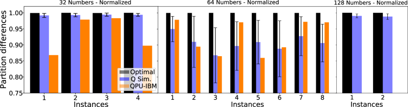
Figure 4: The difference between partition sets for 32, 64 and 128 Numbers. Each instance was run on the quantum simulator 4 times. Each instance was run on the quantum simulator with GA, 100 times for 32 numbers, 10 times for 64 numbers and 4 times for 128 numbers. The QPU data are based on a single run.

As described in Section II.3.1, the number partitioning problem can be directly converted into the Maximum Cut problem. The graphs hence formed are weighted fully-dense graphs.

For the instances, all the numbers used were random integers between 1 and 100. Tests were carried out on the quantum simulator as well as on real hardware from IBM.

The results of partition differences have been normalized in the following manner. For a problem with $N$ numbers, if the partition difference is $p$, then the normalised difference is $p_{norm}=\dfrac{50N-p}{50N}$. All our numbers are random integers between $1$ and $100$, hence $50.5$ on an average. For simplicity we use $50$ in $p_{norm}$.

The optimal value for each instance is obtained using the Integer Quadratic model described in Appendix C.

Figure 4 displays the performance of 32, 64, and 128-number Minimum Partition converted to Maximum Cut. For 32 integers, we have a mean value of $98\%$ and a very small dispersion using the quantum simulator. For 64-number Minimum Partition, the mean values are better than $85\%$ for all instances. Moreover, for both problems sizes, despite the fact that the Minimum Partition problem leads to a complete graph Maximum Cut problem, actual QPUs are able to demonstrate an approximate solution. The problem of size 128 has mean values of about $97\%$ on a quantum simulator.

All QPU runs in this section are done on $ibmq\_mumbai$.

III.3 Maximum Clique as a conversion from Maximum Cut

The Maximum Clique problem can be converted to the Maximum Cut problem by first converting it to the Maximum 2-Sat (II.3.2) and then from the Maximum 2-Sat to Maximum Cut (II.3.3).

After the conversion, a $n$-node Maximum Clique problem requires the solution of a $2(n+1)$-node Maximum Cut. Table 4 shows results for various instances run on a quantum simulator. It is seen that in half of the instances, the best solution is the optimal solution as obtained using numpy. It should be noted that our approach finds a dense subgraph and then removes the nodes with lowest degree iteratively.

Instance	No. of Qubits	No. of Runs	Best Solution	Worst Solution	Av. Solution	Opt. Solution
Size=31, Density=0.3	6	50	4	3	3.38	4
Size=31, Density=0.4	6	50	5	3	3.92	5
Size=31, Density=0.5	6	50	6	3	4.46	6
Size=31, Density=0.6	6	50	7	4	5.34	8
Size=31, Density=0.7	6	50	8	5	6.26	9
Size=63, Density=0.5	7	10	8	6	6.5	8
Size=63, Density=0.6	7	10	8	6	7.2	10
Size=63, Density=0.7	7	10	11	8	9.3	12

Table 4: Maximum Clique results using quantum simulator with GA.

III.4 Maximum Weighted Independent Set using QUBO method

In this section, results of the Maximum Weighted Independent Set problem solved using the QUBO method (section II.4.1) is presented.

For each figure the performance of the algorithm is shown. The data is normalized using the optimal solution found using the commercial CPLEX solver.

Figure 5 shows the data for graphs of size 32, 64 and 128. The data for 32, 64 and 128 nodes is based on 50, 50 and 10 runs respectively. The data represented only takes into account the feasible solutions produced. For graphs of size 32, the mean values for all instances are above $80\%$ and the best obtained result is optimal for every instance. For graphs of size 64, the mean values for all instances are above $60\%$ and the best obtained result is on an average over $80\%$. For 128-node graphs, the solutions are slightly degraded in comparison. Note, however, that the data for 128-node instances is based only on a few runs. Moreover, the performance also depends on the number of GA iterations used in the algorithm run. The number of GA iterations used for the experiments for sizes 32, 64, and 128 are 50, 100 and 200 respectively.

Table 5 shows how the performance varies depending upon the number of GA iterations used. For this table, the Maximum Weighted Independent Set Instance 4 of size 64 has been taken. An increase in the number of GA iterations not only improves the performance but also the percentage of feasible results.

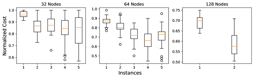
Figure 5: Maximum Weighted Independent Set problem for 32, 64 and 128-node graphs using a quantum simulator. Each instance was run on a quantum simulator with GA 50 times for graph sizes of 32 and 64 and 10 times for graph size of 128.

Size	GA iterations	Solution as % of Optimum	% of Feasible Solutions
64	50	54.8	60
64	100	66.6	96
64	200	77.8	100

Table 5: Maximum Weighted Independent Set results demonstrating the relationship between GA iterations and performance. The Instance 4 of size 64 is used for this table. The performances are an average over 10 runs.

III.5 A comparative study of time taken by the simulator and the QPU

In Table 6 and Figure 6, the time taken to run the algorithm for different Maximum Cut instance sizes is compared. While the quantum computer still takes a significant amount of time to solve the problem, the time taken does not increase exponentially as in the case of the simulator. As we move towards larger instances, we reach a point where it is quicker to run a problem on a QPU than using a simulator.

Note that the QPU time here does not take into account the queue time or waiting time for the QPU runs. The real-world time was several hours or even several days for the largest run instance. This prevented us from running larger instances on the quantum computer.

N	QPU(minutes)	Quantum Simulator(minutes)
32	1.7	3
64	9	52
128	45	222
256	112	3202

Table 6: Data for time taken for various instance sizes in the the QPU and in the quantum simulator

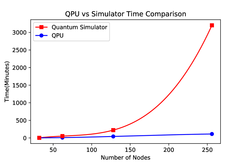
Figure 6: Plot demonstrating the time taken by the quantum simulator versus the time taken to solve the same instance on real hardware

IV Conclusion

In this paper, we investigated and further developed methods to logarithmically encode combinatorial optimization problems on a quantum computer. We begin with expanding the work done in [26], which describes a way to logarithmically encode the Maximum Cut problem. We performed several runs of this algorithm with various instances, on the quantum simulator as well as real hardware, using different classical optimizers like COBYLA and the genetic algorithm.

We then reformulate a number of NP-hard combinatorial optimization problems into the Maximum Cut problem, either directly or indirectly and solve it on a real quantum computer. We take the Minimum Partition problem as an example and solve it by using a reduction as mentioned in section II.3.1. This is possible since the algorithm is largely unaffected by increasing the density of the Maximum Cut graph in question, since the Minimum Partition problem converts into a weighted fully-dense graph. Some performance benchmarks of the partition problem have been presented.

We then proceed to present a more general formulation inspired from the structure of the Maximum Cut algorithm. We see that instead of using the Laplacian, we can use the QUBO matrix of a problem in order to solve it. We introduce the sQUBO representation of the QUBO matrix for it to be compatible with the algorihtm. This therefore opens up the applicability of the algorithm to a wide range of algorithms. The Maximum Weighted Independent Set problem is solved using its sQUBO matrix.

To our knowledge, it is the first time that graph problems of such sizes (256 Maximum Cut, 64 Minimum Partition) have been executed on real universal gate-based quantum computers.

V Declarations

V.1 Ethical Approval and Consent to participate

Not applicable.

V.2 Consent for publication

Not applicable.

V.3 Data availability statement

The authors will make all data available upon reasonable requests.

V.4 Competing interests

A part of the methodology presented in the manuscript is protected by a provisionally patent claim ”Method for optimizing a functioning relative to a set of elements and associated computer program product” submission number EP21306155.9 submitted on 26.8.2021.

V.5 Funding

Y.C. and M.R. acknowledge funding from European Union’s Horizon 2020 research and innovation programme, more specifically the $\bra{\text{NE}}\text{AS}\ket{\text{QC}}$ project under grant agreement No. 951821.

Appendix A Appendix: Calculating the Expectation value of an observable

Given a Hamiltonian matrix $H$, we first need to convert into a sum of tensor products of Pauli strings.

Let $H$ be a $n\times n$ Hamiltonian matrix and $S=\{I,X,Y,Z\}^{n}=\{S_{1},S_{2},S_{3},S_{4}\}^{n}$ be the set of Pauli matrices. We can consider $n$ to be a power of $2$ without any loss of generality. If the size of the Hamiltonian matrix is $n^{\prime}$ which is not a power of $2$, we can easily convert it to a size of $n=2^{\log_{2}(n^{\prime})}$, which is a power of $2$. The extra space in the matrix is filled with $0$’s.

This Hamiltonian can now represented on $N=\log_{2}(n)$ qubits. Consider the set $J=\{S_{i_{1}}\otimes S_{i2}...\otimes S_{iN}|i_{1},i_{2}....i_{N}\in\{0,1,2,3\}\}$ which consists of all tensor product combinations of the Pauli matrices.

Then the Hamiltonian can decomposed as:

$$H=\sum\limits_{i=1}^{4^{N}}c_{i}J_{i}$$ (27)

where the coefficients are:

$$c_{i}=\frac{1}{n}Tr(J_{i}\cdot H)$$ (28)

The Hamiltonian therefore becomes:

$$H=\frac{1}{n}\sum\limits_{i=1}^{4^{N}}Tr(J_{i}\cdot H)J_{i}$$ (29)

The expectation value becomes a sum of the expectation values of all the terms.

$$\bra{\Psi}H\ket{\Psi}=\frac{1}{n}\sum\limits_{i=1}^{4^{N}}Tr(J_{i}\cdot H)\bra{\Psi}J_{i}\ket{\Psi}$$ (30)

Appendix B Appendix: Integer Linear Program for Maximum Cut Problem

Given a graph $G(V,E)$ such that $n=|V|$, and $A_{ij}$ being the corresponding Adjacency matrix terms, we have
Objective : $\max\sum_{1\leq i\leq j\leq n}x_{ij}A_{ij}$
Constraints :

1. $x_{ij}\leq x_{ik}+x_{kj}$

2. $x_{ij}+x_{ik}+x_{kj}\leq 2$

3. $x_{ij}\in\{0,1\}$

Appendix C Appendix: Integer Quadratic Program for Minimum Partition Problem

Given a set $S=\{w:w\in\mathbb{Z}^{+}\}$, and $A\subseteq S$, we have
Variables : $x_{i}=\begin{cases}1\quad&\text{if }\,w_{i}\in A\\ 0\quad&\text{if }\,w_{i}\notin A\\ \end{cases}$
Objective : $\min\big{(}\sum\limits_{i=1}^{n}{w_{i}x_{i}}-\sum\limits_{i=1}^{n}{w_{i}}(1-x_{i})\big{)}^{2}$

References

- Hillar and Lim [2013] C. J. Hillar and L.-H. Lim, Most tensor problems are np-hard, Journal of the ACM (JACM) 60, 1 (2013).
- Woeginger [2003] G. J. Woeginger, Exact algorithms for np-hard problems: A survey, in Combinatorial optimization—eureka, you shrink! (Springer, 2003) pp. 185–207.
- Sánchez-Arroyo [1989] A. Sánchez-Arroyo, Determining the total colouring number is np-hard, Discrete Mathematics 78, 315 (1989).
- Klein and Young [2010] P. N. Klein and N. E. Young, Approximation algorithms for np-hard optimization problems, in Algorithms and theory of computation handbook: general concepts and techniques (UC Riverside, 2010) pp. 34–34.
- Hochba [1997] D. S. Hochba, Approximation algorithms for np-hard problems, ACM Sigact News 28, 40 (1997).
- Bui and Jones [1992] T. N. Bui and C. Jones, Finding good approximate vertex and edge partitions is np-hard, Information Processing Letters 42, 153 (1992).
- Hendrickx and Olshevsky [2010] J. M. Hendrickx and A. Olshevsky, Matrix p-norms are np-hard to approximate if p, SIAM Journal on Matrix Analysis and Applications 31, 2802 (2010).
- Farhi et al. [2014] E. Farhi, J. Goldstone, and S. Gutmann, A quantum approximate optimization algorithm, arXiv:1411.4028 (2014).
- Hadfield et al. [2019] S. Hadfield, Z. Wang, B. O’Gorman, E. G. Rieffel, D. Venturelli, and R. Biswas, From the quantum approximate optimization algorithm to a quantum alternating operator ansatz, Algorithms 12, 10.3390/a12020034 (2019).
- Callison and Chancellor [2022] A. Callison and N. Chancellor, Hybrid quantum-classical algorithms in the noisy intermediate-scale quantum era and beyond, Phys. Rev. A 106, 010101 (2022).
- Peruzzo et al. [2014] A. Peruzzo, J. McClean, P. Shadbolt, M.-H. Yung, X.-Q. Zhou, P. J. Love, A. Aspuru-Guzik, and J. L. O’brien, A variational eigenvalue solver on a photonic quantum processor, Nature communications 5, 1 (2014).
- Moll et al. [2018] N. Moll, P. Barkoutsos, L. S. Bishop, J. M. Chow, A. Cross, D. J. Egger, S. Filipp, A. Fuhrer, J. M. Gambetta, M. Ganzhorn, et al., Quantum optimization using variational algorithms on near-term quantum devices, Quantum Science and Technology 3, 030503 (2018).
- Stokes et al. [2020] J. Stokes, J. Izaac, N. Killoran, and G. Carleo, Quantum natural gradient, Quantum 4, 269 (2020).
- Nakanishi et al. [2020] K. M. Nakanishi, K. Fujii, and S. Todo, Sequential minimal optimization for quantum-classical hybrid algorithms, Physical Review Research 2, 043158 (2020).
- Cerezo et al. [2021] M. Cerezo, A. Arrasmith, R. Babbush, S. C. Benjamin, S. Endo, K. Fujii, J. R. McClean, K. Mitarai, X. Yuan, L. Cincio, et al., Variational quantum algorithms, Nature Reviews Physics 3, 625 (2021).
- Bittel and Kliesch [2021] L. Bittel and M. Kliesch, Training variational quantum algorithms is np-hard, Physical Review Letters 127, 120502 (2021).
- Lubasch et al. [2020] M. Lubasch, J. Joo, P. Moinier, M. Kiffner, and D. Jaksch, Variational quantum algorithms for nonlinear problems, Physical Review A 101, 010301 (2020).
- Mariella and Simonetto [2021] N. Mariella and A. Simonetto, A quantum algorithm for the sub-graph isomorphism problem, arXiv preprint arXiv:2111.09732 (2021).
- Barkoutsos et al. [2020] P. K. Barkoutsos, G. Nannicini, A. Robert, I. Tavernelli, and S. Woerner, Improving variational quantum optimization using cvar, Quantum 4, 256 (2020).
- Tilly et al. [2022] J. Tilly, H. Chen, S. Cao, D. Picozzi, K. Setia, Y. Li, E. Grant, L. Wossnig, I. Rungger, G. H. Booth, et al., The variational quantum eigensolver: a review of methods and best practices, Physics Reports 986, 1 (2022).
- Fuchs et al. [2021] F. G. Fuchs, H. Ø. Kolden, N. H. Aase, and G. Sartor, Efficient encoding of the weighted max k-cut on a quantum computer using qaoa, SN Computer Science 2, 1 (2021).
- Larkin et al. [2022] J. Larkin, M. Jonsson, D. Justice, and G. G. Guerreschi, Evaluation of qaoa based on the approximation ratio of individual samples, Quantum Science and Technology (2022).
- Herrman et al. [2021] R. Herrman, L. Treffert, J. Ostrowski, P. C. Lotshaw, T. S. Humble, and G. Siopsis, Globally optimizing qaoa circuit depth for constrained optimization problems, Algorithms 14, 294 (2021).
- Zhou et al. [2020] L. Zhou, S.-T. Wang, S. Choi, H. Pichler, and M. D. Lukin, Quantum approximate optimization algorithm: Performance, mechanism, and implementation on near-term devices, Physical Review X 10, 021067 (2020).
- Guerreschi and Matsuura [2019] G. G. Guerreschi and A. Y. Matsuura, Qaoa for max-cut requires hundreds of qubits for quantum speed-up, Scientific reports 9, 1 (2019).
- Rančić [2023] M. J. Rančić, Noisy intermediate-scale quantum computing algorithm for solving an n-vertex maxcut problem with log (n) qubits, Physical Review Research 5, L012021 (2023).
- Nielsen and Chuang [2011] M. A. Nielsen and I. L. Chuang, Quantum Computation and Quantum Information: 10th Anniversary Edition (Cambridge University Press, 2011).
- Preskill [2018] J. Preskill, Quantum Computing in the NISQ era and beyond, Quantum 2, 79 (2018).
- Preskill [2021] J. Preskill, Quantum computing 40 years later, arXiv (2021).
- Feynman [1982] R. P. Feynman, Simulating physics with computers, International Journal of Theoretical Physics 21, 10.1007/BF02650179 (1982).
- Hauke et al. [2020] P. Hauke, H. G. Katzgraber, W. Lechner, H. Nishimori, and W. D. Oliver, Perspectives of quantum annealing: Methods and implementations, Reports on Progress in Physics 83, 054401 (2020).
- Stern and Lindner [2013] A. Stern and N. H. Lindner, Topological quantum computation—from basic concepts to first experiments, Science 339, 1179 (2013).
- Briegel et al. [2009] H. J. Briegel, D. E. Browne, W. Dür, R. Raussendorf, and M. Van den Nest, Measurement-based quantum computation, Nature Physics 5, 19 (2009).
- Shor [1999] P. W. Shor, Polynomial-time algorithms for prime factorization and discrete logarithms on a quantum computer, SIAM review 41, 303 (1999).
- Grover [1996] L. K. Grover, A fast quantum mechanical algorithm for database search, in Proceedings of the twenty-eighth annual ACM symposium on Theory of computing (1996) pp. 212–219.
- Kerenidis and Prakash [2020] I. Kerenidis and A. Prakash, A quantum interior point method for lps and sdps, ACM Transactions on Quantum Computing 1, 1 (2020).
- Pothen et al. [1990] A. Pothen, H. D. Simon, and K.-P. Liou, Partitioning sparse matrices with eigenvectors of graphs, SIAM journal on matrix analysis and applications 11(430) (1990).
- Harrigan et al. [2021] M. P. Harrigan, K. J. Sung, M. Neeley, K. J. Satzinger, F. Arute, K. Arya, J. Atalaya, J. C. Bardin, R. Barends, S. Boixo, et al., Quantum approximate optimization of non-planar graph problems on a planar superconducting processor, Nature Physics 17, 332 (2021).
- Winderl et al. [2022] D. Winderl, N. Franco, and J. M. Lorenz, A comparative study on solving optimization problems with exponentially fewer qubits, arXiv preprint arXiv:2210.11823 (2022).
- Bezdek and Hathaway [2002] J. C. Bezdek and R. J. Hathaway, Some notes on alternating optimization, in AFSS international conference on fuzzy systems (Springer, 2002) pp. 288–300.
- Karp [1972] R. M. Karp, Reducibility among combinatorial problems, In: Miller, R.E., Thatcher, J.W., Bohlinger, J.D. (eds) Complexity of Computer Computations. The IBM Research Symposia Series. Springer, Boston, MA. (1972).
- Ruiz-Vanoye et al. [2011] J. A. Ruiz-Vanoye et al., Survey of polynomial transformations between np-complete problems, Journal of Computational and Applied Mathematics 235, 4851 (2011).
- Glover et al. [2019] F. Glover, G. Kochenberger, and Y. Du, Quantum bridge analytics i: a tutorial on formulating and using qubo models, 4OR, Springer 17(4), 335 (2019).
- de la Vega and Kenyon-Mathieu [2007] W. F. de la Vega and C. Kenyon-Mathieu, Linear programming relaxations of maxcut, in Proceedings of the Eighteenth Annual ACM-SIAM Symposium on Discrete Algorithms, SODA ’07 (Society for Industrial and Applied Mathematics, USA, 2007) p. 53–61.
- Goemans and Williamson [1995] M. X. Goemans and D. P. Williamson, Improved approximation algorithms for maximum cut and satisfiability problems using semidefinite programming, Journal of the ACM (JACM) 42, 1115 (1995).