Critical avalanches of Susceptible-Infected-Susceptible dynamics in finite networks
Abstract
We investigate the avalanche temporal statistics of the Susceptible-Infected-Susceptible (SIS) model when the dynamics is critical and takes place on finite random networks. By considering numerical simulations on annealed topologies we show that the survival probability always exhibits three distinct dynamical regimes. Size-dependent crossover timescales separating them scale differently for homogeneous and for heterogeneous networks. The phenomenology can be qualitatively understood based on known features of the SIS dynamics on networks. A fully quantitative approach based on Langevin theory is shown to perfectly reproduce the results for homogeneous networks, while failing in the heterogeneous case. The analysis is extended to quenched random networks, which behave in agreement with the annealed case for strongly homogeneous and strongly heterogeneous networks.
I Introduction
Systems undergoing continuous absorbing-state phase-transitions are, exactly at the critical point, infinitely susceptible to local perturbations. This implies that, introducing a single active seed in the absorbing state, the subsequent evolution leads to an avalanche of activation events that may span the whole range of temporal and spatial scales. Examples of this avalanche dynamics abound, both in the realm of physics and in other biological, social and technical domains [3, 4, 5, 6, 7, 8, 9].
The multiscale nature of these phenomena is quantitatively characterized by the size and duration distributions of avalanches. If the control parameter is subcritical (i.e., in the absorbing phase) size and duration of avalanches are exponentially distributed, extending up to well defined and finite temporal and spatial scales. In the supercritical domain, instead, a finite fraction of them spans the whole system, leading (in infinite systems) to a stationary active state. In the critical case all avalanches end in a finite time, but the distributions have power-law tails so that events of any size and duration are possible. Denoting with the size of an avalanche and with its duration, we can in general write for the probability distributions of size and duration [10]
| (1) |
where and are universal critical exponents, and are scaling functions and the cutoff scales and depend at criticality only on the system size. Averaging the avalanche size at a fixed duration it is possible to define another exponent , which is related to the others as [11]
| (2) |
The branching process (BP) model [12] provides the natural framework for describing (at least approximately) a large class of systems undergoing continuum absorbing phase transitions. In the simplest case, when the distribution of offsprings (i.e., the probability for an active element to activate a given number of new elements) has finite variance, BP theory predicts
| (3) |
This kind of mean-field behavior is expected to occur when the system dynamics takes place on a homogeneous network, where the second moment of the degree distribution is finite. The phenomenology changes when the distribution of offsprings in the BP has infinite variance, as it happens for processes taking place on heterogeneous networks with degree distribution and . In such a case BP theory predicts anomalous, -dependent, exponents [13, 14, 15, 16]
| (4) |
While standard BP behavior is observed for many systems on homogeneous networks [17, 18, 19, 20], recent work has cast doubts over the applicability of this theoretical framework to many avalanche phenomena in heterogeneous networks [21]. In all cases considered, apart from a possible preasymptotic regime valid for short duration and small size, the distributions decay with exponents in agreement with standard BP values, with no dependence on . Possible causes of this violation of the BP predictions have been put forward in Ref. [21]. One possible reason for such violation is the existence of loops in networks, possibly allowing for nodes that are already active to be reached again by the infection, which is an explicit violation of the mapping between spreading models and the BP. Further, finite networks always have a finite second moment of the degree distribution, which prevents the anomalous exponents (4) to be asymptotically observed even in a pure BP. It was also noted in Ref. [21] that the spreading mechanism of certain models, such as the contact process (CP), do not really involve all the neighbors of a node and hence avalanches are not impacted by unbounded fluctuations of the network degree distribution. These hypotheses, however, call for more detailed investigations of the origin of the breakdown of anomalous BP exponents in specific systems and for the formulation of alternative theoretical approaches such as the one presented in Ref. [22]. Also, the way avalanches depend on the system size in finite systems, which is an issue of crucial importance for the analysis of real systems, is still largely unexplored.
In this work we consider Susceptible-Infected-Susceptible (SIS) dynamics [23], one of the most fundamental (and simple) models deemed to be described by BP, and perform such an investigation in complex networks of variable size. Apart from the intrinsic importance of SIS dynamics, an additional motivation for our study is that it has been realized that the interplay between heterogeneous topology and SIS dynamics gives rise to highly nontrivial phenomena, such as the vanishing of the threshold in the large-network limit [24, 25, 26], the interplay between distinct subextensive subgraphs [27] and long-range percolation effects [28]. Whether and how these nontrivial properties of the stationary state are reflected also in the avalanche statistics and its dependence on the system size are other aspects deserving to be analyzed.
Our investigation is inspired by the work of Ref. [29] that deals with critical properties of the CP, a model akin to SIS, but exhibiting simpler critical dynamics characterized by a finite threshold for any value of . For CP, avalanche exponents are nonanomalous also for , but this is easily reconciled with the BP phenomenology, as the effective distribution of the number of offsprings does not depend on the network substrate and is always homogeneous. Yet, Ref. [29] presents a detailed analytical investigation of CP based on a Langevin approach, which constitutes the natural basis also for the analytical approach to SIS avalanches and in particular for their temporal properties.
In this paper we perform numerical simulations of the critical SIS model on annealed and quenched networks, both homogeneous and heterogeneous, generated according to the configuration model (CM) [30]. We further develop a theoretical approach based on the use of Langevin equations to study the probability that avalanches have duration at least . The theoretical approach explicitly makes use of the annealed network approximation, but we show that it further provides with a partial understanding of the avalanche behavior on quenched networks. The rest of the paper is organized as follows. In Section II, the dynamics of the SIS model and the statistical features of the networks we consider are briefly introduced. In Section III, we summarize the phenomenology we observe on different network structure, and offer a clear physical interpretation of the avalanche behavior. In Section IV, numerical results for annealed networks are discussed. In Section V, the theoretical approach is presented and its predictions are compared with the results of the previous section. In Section VI, results for quenched networks are shown and compared to the theoretical predictions of the previous section. We discuss our results Section VII.
II Model definitions
Spreading dynamics
We consider the continuous-time Susceptible-Infected-Susceptible (SIS) dynamics on networks. Each node can be either infected (I) or susceptible (S). Infection events, i.e., , occur according to a Poisson process with rate . Recovery events, i.e., , obey a spontaneous Poisson process with rate . We set , with no loss of generality. The configuration where all nodes are in the S state is an absorbing configuration: once such a configuration is reached the system will remain in it forever, as no new infections can arise. In a network of infinite size, if the dynamics is started from a configuration different from the absorbing one, a critical value of the control parameter separates a phase where the system unavoidably reaches the absorbing configuration (i.e., ) from a phase where a stationary state with a finite fraction of infected nodes exists ( ).
On a network with finite size , the SIS model does not undergo a true phase transition. As long as the rate of infection is finite, the system necessarily ends up in the absorbing configuration in a finite time. Nonetheless, it is still possible to identify a pseudo-critical point , distinguishing a phase where the system reaches the absorbing configuration in a time that, on average, grows at most logarithmically with the system size (i.e., ), and a phase where the absorbing configuration is reached in an average time that grows exponentially with the system size (i.e., ).
In this paper, we are interested in characterizing SIS spreading on networks of finite size in their pseudo-critical regime, i.e., . We perform a large-scale numerical analysis and develop a theoretical approach valid for a specific initial setup where infected nodes are surrounded by a completely susceptible system. Our main goal is understanding in detail the behavior of the survival probability , i.e., the probability that the system has not yet reached the absorbing configuration by time , connected to the duration distribution as . To avoid verbosity, we refer to the critical regime even if a network has finite size. Also, we make use of the compact notation instead of to indicate the pseudo-critical point of a network with finite size .
Networks
As interaction patterns, we consider networks built according to the CM [30]. The properties of a network generated according to the CM are specified by its degree distribution, i.e., the probability that a randomly selected node has degree . Each quenched network realization of the CM is obtained by sampling the degree sequence from and pairing nodes in a completely random manner, while preserving the degree sequence. The only constraint we set on the pairing procedure is that multiedges and self-loops are prohibited. The -th sample moment of the degree sequence is given by
| (5) |
The annealed version of the CM model implies that a new pairing is generated at each time step, still keeping the degree sequence fixed. In the annealed scenario one can usefully define the annealed adjacency matrix as the average over all possible pairings: . Its elements equal the probability that a node of degree is connected to a node of degree [31].
In this work, we focus on power-law degree sequences generated by selecting random variates from the distribution
| (6) |
In the following, without loss of generality, we set , however, results are qualitatively similar for , as long as is independent of . We assume that the maximum degree is growing as a power of , i.e.,
| (7) |
with
| (8) |
This specific setting of the CM model is known as the uncorrelated configuration model (UCM) [32]. Imposing the constraints of Eqs. (7) and (8) provides several advantages. For example, one can safely assume that the effective maximum degree observed in the sequence sampled from is actually if is sufficiently large [29]. Also, quenched UCM networks have negligible degree-degree correlations.
Using the above constraints, one finds that the -th moment of a large but finite network scales approximately as
| (9) |
For , the power-law degree distribution of Eq. (6) has diverging second moment, i.e., for . We refer to networks in this class as heterogeneous networks. For instead, is finite, and we refer to this class as homogeneous networks.
III Summary of the results
We consider SIS dynamics on a finite network of size initialized with infected nodes. The sum of the degrees of the seeds is . The survival function turns out to be characterized by three main regimes describing respectively short, intermediate and long avalanches. We denote the point of transition between the first two regimes as and the point of transition between the second and third regime as . The transitions between the various regimes are not sharp, rather the survival function displays smooth crossover behaviors. This qualitative behavior is valid irrespectively of the exponent of the degree distribution in Eq. (6). Also, both the quenched and the annealed versions of the UCM exhibit this qualitative behavior. However, fundamental differences between homogeneous and heterogeneous networks exist as the actual values of the transition points depend on the degree exponent .
III.1 Regime of short avalanches
For , in the regime of short avalanches, the survival function of each of the avalanches is characterized by an exponential decay. This is due the immediate recovery of each of the initial spreaders. The characteristic time scale of the exponential decay is equal to 1 because we set the rate of recovery as . If the avalanches are small enough not to interact one with the other, we can write , i.e., the survival probability equals the probability that at least one of the avalanches is still active at time . Such expression behaves as
| (10) |
if is sufficiently large. In particular, the above expression must be at most 1 so it can hold only if .
The relative weight of the regime of short avalanches compared to the other regimes valid for longer avalanches, which ultimately determines the transition point , strongly depends on the initial condition of the dynamics and the topology of the underlying network. If , then does not display any dependence on the network size; if, instead, , a logarithmic divergence of with the system size appears. For , the fraction of trajectories that ends in this regime also depends on the initial condition. If the spreading is initiated by spreaders with a sufficiently large , then and the regime is barely visible, while grows as diminishes.
III.2 Regime of intermediate avalanches
The range is known as the adiabatic regime [29, 21]. This regime describes avalanches that are sufficiently long to have lost any memory of the initial conditions. The survival function decays as
| (11) |
The power-law decay with exponent is typical of critical spreading on networks with finite second moment of the degree distribution [17, 21, 22]. Here we find that the same decay describes intermediate avalanches in finite networks characterized by degree distributions with diverging second moment.
III.3 Regime of long avalanches
Finally, avalanches that last are sufficiently large to feel the finite size of the network. An exponential cutoff characterizes the decay of the survival function in this regime, i.e.,
| (12) |
In particular, we have that the typical time of the exponential cutoff diverges as a power of the network size, i.e.,
| (13) |
The specific value of depends on and only if ; otherwise.
IV Numerical results for annealed networks
In this section, we consider the case of uncorrelated annealed networks [29]. We consider the critical dynamics, setting , the exact epidemic threshold for uncorrelated networks. We consider networks of finite size, and therefore the scaling of and with , is the one in Eq. (9). It follows that, for , for ; instead, does not vanish for if [23].
IV.1 Homogeneous networks
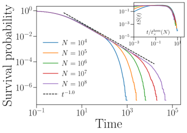
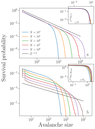
Figure 1 shows results obtained by simulating critical SIS dynamics on homogeneous networks generated via the CM with , and . All realizations have been initiated with a single infected node, i.e., , of degree , where is the floor function. This choice is motivated by the need of having an initial condition that is independent of the system size.
The three regimes anticipated in the summary above are clearly visible. Given the homogeneity of the network, short avalanches do not display any dependence on the network size. This is the standard behavior of the continuous-time BP [33] and hence it is not surprising to observe it on homogeneous networks. In particular, we observe . In the regime of intermediate avalanches, the survival probability shows the power-law decay of Eq. (10). The exponential cutoff emerges after a time
| (14) |
This is apparent from the finite-size scaling analysis shown in the inset of Fig. 1. This fact is consistent with what one finds for other critical spreading processes on homogeneous networks via a standard mean-field description [34].
The standard mean-field picture emerging from the analysis of the SIS model on homogeneous networks is further confirmed by the fact that the probability distribution of the avalanche size scales with exponent and shows a cutoff diverging linearly with the system size, see Appendix A. Both these results are consequences of the behaviour of and of the scaling law that relates the average avalanche size with its duration [17].
IV.2 Heterogeneous networks
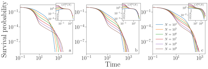
Results for heterogeneous networks with degree exponent are shown in Figure 2. Also in this case, all realizations have been initiated with infected node of degree . Despite Eq. (9) predicts const. for any , in small systems such as the ones that can be considered numerically, has not yet reached its limit value and displays a slow dependence on . The three qualitative regimes are still present, but the crossovers between the various regimes strongly depend on and , in stark contrast with the homogeneous problem.
Short avalanches are described by the exponential decay of Eq. (10). We observe that grows as increases. The reason for such a behavior is quite intuitive. The critical value of the epidemic threshold goes to zero as the system size increases. However, the initial condition of the dynamics is unaffected by the network size, as we are still considering spreading processes initiated by nodes with degree . Many configurations generate short avalanches just because the probability of observing spreading events instead of recoveries becomes negligible as the size of the network increases. For example, the probability that the first event is a spreading event is , which clearly goes to zero as the system size increases.
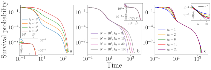
This physically intuitive picture can be made more precise by studying the dependence of the survival function in the regime of short avalanches on the initial condition of the dynamics. Our main finding in this regard is that the crossover from the exponential to the power-law decay starts when the survival probability has dropped by an amount that we infer to scale as . This finding is deduced from the combination of the results of Figs. 3a, 3b and 3c. In Fig. 3a, we start the dynamics from a single initial seed, i.e., with variable degree . Simulations are all performed on the same network, thus is constant. The drop of is proportional to , as apparent from the inset of Fig. 3a. In Fig. 3b instead, we consider networks of different size to keep the ratio constant. In the regime of short avalanches, the different curves collapse with no rescaling. Finally, in Fig. 3c, we vary the number of initially infected nodes , but keep constant the sum of their degrees: . The value of the initial drop of is once again constant, as the ratio is not varied. The value of the time appears the same for all settings. For , the functional form of depends linearly on , as described by Eq. (10).
The scaling of the initial drop of the survival function together with the known exponential decay characterizing in the regime of short avalanches, i.e., Eq. (10), and the imposed dependence of the maximum degree, i.e., Eq. (7), allow us to write that
| (15) |
thus a logarithmic growth of the time distinguishing short from intermediate avalanches.
Intermediate avalanches are perfectly described by the power law of Eq. (11). Our finite-size scaling analysis indicates that
| (16) |
The scaling of Eq. (16) is clearly different from the one predicted for homogeneous networks, i.e., Eq. (14). It can be, however, linked to the same physical interpretation behind Eq. (14) using the known fact that in the SIS model on annealed networks, at criticality, the subset of nodes with largest degree plays a crucial role [23]. For , this set is subextensive, and contains the nodes with largest degree [35]. The subgraph of the nodes with largest degree is also known to be homogeneous, in the sense that the smallest, largest and average degree of this subgraph all scale in the same way with the system size, as in homogeneous networks [35]. As a matter of fact, we can interpret the finding of Eq. (16) as , thus as the cutoff time valid for a homogeneous graph, i.e., Eq. (14), with nodes. Note that Eqs. (15) and (16) explicitly depend on [see also Eq. (7)]. The validity of these expressions as is varied is assessed in Appendix B.
V Langevin theory for annealed networks
The striking differences between the two cases of homogeneous and heterogeneous networks call for an analytical investigation. A natural choice for this task is to develop a theory based on a Langevin equation for the order parameter. The general theory of stochastic processes [36] provides with an exact protocol to compute given a Langevin equation for the order parameter and such a protocol has been successfully employed to describe the behaviour of avalanches in the CP [29]. Inspired by Ref. [29], we develop a theoretical approach for the SIS model on annealed networks.
For annealed networks the degree sequence fully determines the network properties: nodes with the same degree have exactly the same dynamical behavior. It is therefore convenient to define the variables and which represent, respectively, the number of infected nodes with degree at time and the probability that a randomly selected node among those with degree is infected at time . The epidemic phase transition can be described through the order parameter , representing the probability that a random node is infected, or through the order parameter , representing the probability that a random neighbor of a node is infected.
The theoretical approach is based on the observation that the variables , and hence , are sums of a large number of binary random variables, which for annealed networks are independent [29]. Appealing to the central limit theorem, the temporal evolution of these variables can be described by means of suitable Langevin equations.
Following closely the approach of Ref. [29] valid for the CP, we find the Langevin equation valid for the critical SIS model is
| (17) |
where is a Gaussian white noise of zero mean and unit variance. The derivation of this result is in appendix C, and is based on three main hypotheses. We assume that the dynamics takes place on an annealed uncorrelated network, the variables evolve in time subjected to Gaussian white noise and, importantly, the adiabatic approximation is valid.
Such an approximation consists in replacing the value of the microscopic variables in the equation for the evolution of the order parameter with quasi-stationary, -dependent, values, obtained by setting the time derivative to zero in their evolution equations. This is based on the fact that evolves slowly at criticality, while the relax exponentially fast. (see Appendix C). Only sufficiently long avalanches may be correctly described by our theory. In particular, the Langevin theory can not explain the regime of short avalanches, where the exponential decay is observed. This happens because the adiabatic approximation is not yet valid.
Eq. (17) can be recast as a partial differential equation for , which in turn can be used to compute the finite-size properties of the survival function. Explicit calculations are shown in Appendix D. At criticality, the theory predicts
| (18) |
where
| (19) |
and with a cutoff for long times, due to the finite size of the network, scaling as
| (20) |
For , Eq. (18) predicts that . This prediction is valid for all networks, homogeneous and heterogeneous, and is in agreement with the results of numerical simulations. We stress that does not represent the same quantity as : the regime of short avalanches is not described under the adiabatic approximation which we do not expect to be valid during the regime of short avalanches. Indeed, the cumulative probability of Eq. (18) equals one for , as expected for a conditional probability such as the present one. in Eq. (18) is conditioned on being larger than the adiabatic relaxation time. The fact that tends to zero in heterogeneous networks signals that the power-law decay begins immediately after the adiabatic relaxation time while it happens after a time that grows with in homogeneous networks.
For homogeneous networks, Eq. (19) predicts of order and Eq. (20) tells us that . These predictions are perfectly consistent with the numerical results presented in section III.
Predictions, however, are only partially in agreement with numerical simulations for heterogeneous networks. The scaling predicted in Eq. (19) is consistent with the fact that is constant, see Fig. 2 and Fig. 3b. The theory, however, incorrectly predicts the scaling of the cutoff for large times . Indeed, for both and diverge as described in Eq. (9), and Eq. (20) gives , which diverges with only if and limits to zero otherwise. This latter finding is not only in stark contrast with the results of the numerical simulations, but is also unphysical, denoting some underlying shortcoming of the theory. We believe that the Langevin approach fails because it assumes the whole system to be involved in the critical dynamics and it does not capture the special role played by the subextensive graph of nodes with highest degree, as explained in the previous section. Hence, we can recover a correct scaling of by heuristically replacing with and using the scaling of the homogeneous problem.
VI Numerical results for quenched networks
The comprehension of the phenomenology on annealed networks allows us to interpret what happens in spreading experiments on quenched networks.
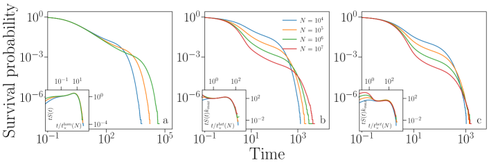
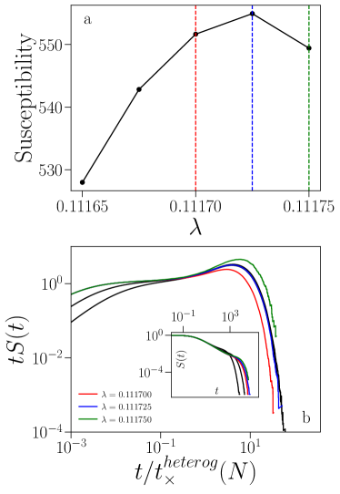
The main limitation to study large-scale networks is the computational cost of estimating the critical threshold of a network. At odds with the case of annealed networks, is not simply given by the ratio between first and second moment of the degree sequence, rather it requires to be numerically estimated [37]. We use the standard practice of identifying as the value corresponding to maximum of the susceptibility associated to , see Appendix E. Numerical estimates of require high accuracy, up to six decimal digits111The number of digits required to have satisfactory results depends on the network., and these estimations are computationally demanding even though the maximization is performed using the efficient quasi-stationary method [37]. We have been able to study networks of size at most . Once, the value of is estimated, spreading experiments for can be performed at a relatively small computational cost.
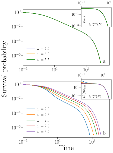
Results of our analysis are shown in Fig. 4. We first validate our method on random regular graphs, whose phenomenology is expected to be perfectly consistent with the standard mean-field picture, i.e., consistent with the predictions of the Langevin theory for homogeneous networks and the findings for homogeneous annealed networks (Fig. 1). Numerical results, shown in Figure 4a, confirm this expectation as obeys Eq. (18) and the cutoff is given by Eq. (20). Interestingly, the scaling function displays a hump just before the cutoff. The hump is sufficiently large to be observed even in the non-rescaled data and hinders the direct observation of the exponent for relatively small systems, a fact that often happens when scaling functions display large peaks [11].
The results for small values of are perfectly analogous to those obtained for heterogeneous annealed networks. For example, in the case , Fig. 4b, one finds that the rescaling used for annealed networks leads to the clean data collapse shown in the inset. This finding is not surprising, as the theory of annealed networks suits well SIS on quenched networks as long as [37, 35]. In Appendix E we show that the maximization of the susceptibility is a necessary step in order to obtain clean-cut results as the ones shown in Fig. 4.
The rescaling used for annealed networks works quite well also for (see Fig. 4c). Also in this case we find that the drop of at small is proportional to and the cutoff is again given by Eq. (16). However, this agreement is valid for the relatively small network sizes we can simulate, i.e., . Based on the findings of Refs. [37, 35, 28], we expect that, for any value , the theory for annealed networks is no longer able to describe critical SIS avalanches on sufficiently large quenched networks, and that a scaling different from Eq. (16) holds for .
VII Conclusions
In this paper we have performed a thorough analysis of SIS critical avalanche dynamics on random networks of finite size. While for annealed homogeneous networks the theoretical understanding is complete and quantitative, when the dynamics takes place on annealed heterogeneous substrates we have to resort to heuristic arguments to correct some shortcomings of the Langevin approach. In particular, it is necessary to assume that nodes play different roles depending on whether they are part of the subextensive subgraph of size which includes high-degree nodes. Such a network subset is where the principal eigenvector of the adjacency matrix gets localized [35]. For stationary properties of the SIS dynamics, this localization determines the position of the epidemic threshold, but it does not affect the probability that a node is infected, which is proportional to the degree for any value of . Our results show instead that for nonstationary properties, such as avalanche statistics, localization matters: nodes outside the subset play no role in the evolution of long avalanches and as a consequence the Langevin approach, which treats all nodes on the same footing, fails.
This failure is in stark contrast with what happens for the CP. Physically, the CP differs from the SIS model as node spreads activity with rate regardless of its degree, rather than spreading with rate . As a consequence, the critical point of the CP is , i.e., is network independent while the critical point of the SIS is not and, in particular, it vanishes in heterogeneous networks. However, the structure of the Langevin equations describing the two processes is quite similar. The equations for the variables are the same, with the only difference that the order parameter appearing in Eq.( 22) is replaced by the factor and Eq.( 23) has the same structure as of the equation for in the CP, with the fundamental difference that the non-linear term involves in the CP, while it involves in the SIS. This difference reflects the physically different spreading mechanisms of the two models. Furthermore, the analogy between the equations for the and for the order parameters allows to perform the adiabatic approximation in both cases and the stationary values of the have indeed the same form. It follows that the closed-form expressions of the Langevin equations are the same for both processes. The physical difference between the two processes, however, is reflected by a different scaling of the drift and diffusion coefficients with the system size. In particular, in the limit of small order parameter, the SIS model involves moments of up to the third (see Eq. (17)) while the highest moment in the CP is the second. Once the Langevin equations are obtained, writing the partial differential equation for , its limit for large and its integration for the calculation of proceeds analogously for both models. It was found that the CP is always characterized by a that does not scale with the system size regardless of the network (as is finite on any network). The cutoff time , however, is correctly predicted for the CP but not for the SIS. A solid mathematical framework to explore this regime is still to be found.
We have verified that, for , the avalanche statistics on quenched networks is practically identical to the case of annealed networks, in agreement with what occurs for stationary properties [37]. For larger values of the stationary properties of SIS on quenched networks (such as the value of the epidemic threshold) are governed by the interplay of hubs which effectively “interact at distance” giving rise to long-range percolation patterns [28]. The investigation of how these highly nontrivial effects influence critical avalanche statistics for quenched networks with remains a very challenging open problem both from the numerical and from the analytical point of view.
Acknowledgements.
F.R. acknowledges support by the Army Research Office (W911NF-21-1-0194) and by the Air Force Office of Scientific Research (FA9550-21-1-0446). The funders had no role in study design, data collection and analysis, decision to publish, or any opinions, findings, and conclusions or recommendations expressed in the manuscript.Appendix A Avalanche size distribution
Figure 5 displays the avalanche size distribution obtained on annealed networks. As explained in the main text, the power-law exponent is easily understood from Eq. (11) and from the quadratic growth of the average avalanche size with the avalanche duration [17]. The avalanche size cutoffs for both classes of networks are understood again using and in particular they are the square of the cutoffs of the survival probability. The drop of for small values of in heterogeneous networks mirrors the exponential decay of the first temporal regime. During such a decay, avalanche size and duration scale linearly as, for short avalanches, an infection event increasing by 1 generally increases only of the healing time of the newly infected node, i.e., on average. Hence, for short avalanches . It follows that the rescaling is the same for both observables.
Appendix B The role of the upper cutoff of the degree distribution
The cutoff is predicted to depend only on in homogeneous networks, Eq. (14), while it explicitly depends on and in heterogeneous networks, Eq. (16). The relation between and is explicitly assessed in Fig. 2. Figure 6 verifies the relationship between and by keeping all parameters fixed except for . For large values, networks are homogeneous regardless of the value. For heterogeneous networks, in turn, depends on , and [38].
Appendix C Derivation of the Langevin equations
The derivation of the Langevin equations proceeds in the same way as in [29, 21]. The Langevin equations for the variables are
| (21) |
Diving by we obtain
| (22) |
and using the definition of
| (23) |
Note that the leading order in Eq. (22) is linear in regardless of the value of , implying a fast exponential decay toward their asymptotic (average) values, while linear terms are suppressed in Eq. (23) by setting and hence is a slowly varying variable at criticality. Therefore, the adiabatic approximation can be performed at the critical point. Setting and yield
| (24) |
In the above expression, the stochastic term vanishes in the thermodynamic limit. Therefore we can rewrite Eq. (24) by replacing in the square root with its leading (deterministic) term, so to express entirely as a function of , obtaining
| (25) |
Replacing this expression in the deterministic term of Eq. (23) gives
| (26) |
while the stochastic term takes the form
| (27) |
The overall contribution to the new stochastic term in the equation for is
| (28) |
Note that, in inserting the sum into the square root, we also replace the individual noises with an overall noise by means of the central limit theorem. Defining and summing and subtracting the quantity , the closed-form of the Langevin equation for is
| (29) |
where
| (30) |
The two summations above can be easily performed if . Under this assumption we have and . Replacing these expressions in Eq. (29) we obtain Eq. (17). Figure 7 shows that the assumption holds if the dynamics is initialized with sufficiently small values of , as we always do in our simulations.
Appendix D The survival probability function
From Eq. (17) an equation for can be derived using standard techniques [36]
| (31) |
with the boundary conditions
| (32) |
expressing the absorbing nature of the barrier in and the reflecting nature of the barrier in . The initial condition on explicitly depends on the system size as . We are interested in deriving the decay of over time and this requires the thermodynamic limit to be taken, so we need an initial condition that does not depend on the system size [29]. We change variable from to . In this way, if we fix the initial condition to be such that only a single node with degree is infected, then . We obtain
| (33) |
where now the thermodynamic limit can be taken. The coefficient of the drift term scales as
| (34) |
if while it scales as if . Analogously, the diffusion coefficient scales as
| (35) |
if and it converges to a constant for .
For we have a “standard” (in the sense of Ref. [17]) diffusive scenario where the drift term tends to zero (for any ) and the diffusion coefficient converges to a constant. For the diffusion coefficient diverges and the drift term again tends to zero unless , which is impossible if . This condition is always met in our numerical simulations when . It follows that for large the dynamics is dominated by the diffusion term, for both homogeneous and heterogeneous networks, in complete analogy with the CP [29]. In the limit of large but finite the drift term can be neglected and the solution to the resulting equation is Eq. (18).
The finite-size cutoff of can be estimated from the average duration of avalanches [29]. For it to be computed, we first need to compute . Integrating in time Eq. (33) we obtain
| (36) |
with boundary conditions, obtained integrating Eqs. (32), given by and , where is the total number of edges. The solution is given by
| (37) |
as can be verified by direct substitution.
Defining and integrating again Eq. (33) we get
| (38) |
The solution is given by
| (39) |
with
| (40) |
For large we can approximate the upper limit of the outer integral in Eq. (39) with 0 and noting that diverges we get
| (41) |
so that the size-dependent cutoff time scales according to Eq. (14) if is asymptotically finite (), while it scales as Eq. (20) if .
Appendix E Determination of the critical point in quenched networks
Figure 8 shows the importance of a precise estimation of the critical point on quenched networks. Figure 8a shows the susceptibility obtained on a random graph with as is varied. The critical point is determined as the value of the spreading rate that maximizes the susceptibility, marked by the blue dashed line. Figure 8b shows three curves obtained using three different values of , the critical one and the two closest values for which we studied the susceptibility (resolution set to ). Despite the curves look extremely similar (inset), the data collapse is strongly impacted by . Figure 8b shows this by slightly increasing or decreasing with respect to to the critical value.
References
- [1]
- [2]