Position prediction using disturbance observer for planar pushing*

Abstract

The position and the orientation of a rigid body object pushed by a robot on a planar surface are extremely difficult to predict. In this paper, the prediction problem is formulated as a disturbance observer design problem. The disturbance observer provides accurate estimation of the total sum of model errors and external disturbances acting on the object. From the estimation results, it is revealed that there is a strong linear relationship between the applied force or torque and the estimated disturbances. The proposed prediction algorithm has two phases: the identification & the prediction. During the identification phase, the linear relationship is identified from the observer output using a recursive least-square algorithm. In the prediction phase, the identified linear relationship is used with a force plan, which would be provided by a mission planner, to predict the position and the orientation of an object. The algorithm is tested for six different push experimental data available from the MIT MCube Lab. The proposed algorithm shows improved performance in reducing the prediction error compared to a simple correction algorithm.

I Introduction

The position and the orientation of a rigid body object pushed by a robot on a planar surface are extremely difficult to predict. The stochastic nature of physical interactions, [1], between objects, surfaces and robots makes an accurate prediction of the position and orientation extraordinary challenging. There are abundant researches on this topic in the past and the current and a few directly related ones to the problems studied in this paper are mentioned in the following.

A nonlinear optimisation problem is solved in [2] to identify the inertial parameters and the contact forces of multiple rigid bodies in a plane with unknown frictional forces, while the contact geometries are assumed to be known. A hybrid model combined an analytical model with a convolutional neural network is presented in [3] for predicting the transnational and rotational motions of an object in a planar pushing, where the position and velocity information of the pusher is used. One of the crucial assumption of the algorithm is a quasi-steady state of the motion. Its prediction performance is degraded for different shape objects or high push velocities. In [4], a state estimation problem for a planar object motion is solved using visual and tactile sensor measurements. This algorithm, however, does not have any prediction part.

These studies focused on understanding of the push dynamics, combining a dynamic model with the machine learning algorithm, or applying purely the machine learning algorithm. In this paper, it is formulated as a disturbance observer design problem. Disturbance observer is one of the widely used control methods. It is mainly used to compensate the influences of external disturbances and parametric uncertainties in a system to achieve robustness towards those perturbations and recover a desired performance. A survey for various disturbance observers is found in [5].

A disturbance observer called Q-filter is adopted in this paper, which was first presented in [6]. The first Q-filter observer is used to estimate disturbances and uncertainties in a DC motor control. It showed promising performances becoming one of the most popular methods for compensating disturbance effects. Stability and robustness of the Q-filter based disturbance observer is presented in [7]. It is not possible, however, that the disturbance observer is simply deployed for the push prediction problem as the observer provides only the current estimation. A prediction algorithm based on the estimated disturbances is required.

This paper is organised as follows: firstly, the push data from the MIT MCube lab is introduced [8], six test scenarios are chosen, and the total force applied is estimated; secondly, a disturbance observer is designed for estimating unknown forces, a prediction algorithm for position & orientation prediction is presented, and the performance of the prediction algorithm is demonstrated using the test scenarios; and, finally, discussions & future work are presented.

II Push Data & Pre-Processing

In this section, the push data available from the MIT MCube lab is introduced and pre-processed. The equation of motions for the translation and the rotation are derived, and the total force and torque applied to an object are identified.

II-A Push Data

The MIT MCube lab performed planar push experiments using a robot arm for various shape of objects, types of surfaces, while the position and the orientation of the pusher, the force experienced in the tip of the pusher, and the position and the orientation of the objects are recorded with 250 Hz [1]. There are total around 6,000 experimental cases and these data are open to download from [8].

TABLE I: Push Data Cases

Case #	acceleration [m/s2]	velocity [m/s]
1	0.0	0.01
2	0.0	0.01
3	0.0	0.01
4	0.0	0.05
5	0.2	-0.001
6	2.5	-0.001

TABLE II: Push Data Measurements

Measurements	Definitions
${\bf r}^{\{\text{rbt}\}}_{\text{C}}$	the tip position in $\{\text{rbt}\}$
$\theta_{\text{tip}}$	the tip orientation with respect to $\{R\}$
${\bf r}^{\{\text{R}\}}_{\text{O'}}$	the object centre position in $\{\text{R}\}$
$\theta$	the object orientation with respect to $\{R\}$
$-{\bf f}^{\{\text{rbt}\}}_{\text{C}}$	the reaction force measured at the tip in $\{\text{rbt}\}$
$-T^{\{\text{rbt}\}}_{\text{C}}$	the reaction torque measured at the tip in $\{\text{rbt}\}$

In this paper, six experiments shown in Table I are chosen for testing algorithms to be proposed in the next section. The experiments include zero acceleration and non-zero acceleration of the pusher with three different velocities of the pusher. The object of the chosen experiments called rec2 is a rectangular shape, whose width and length are 90 mm and 112.5 mm, respectively, [8, 9]. The surface type is the same for all six experiments called abs [1], whose friction coefficient is between 0.13 and 0.15. The available measurements are summarised in Table II.

The tip position of the robot arm in the robot frame, ${\bf r}^{\{\text{rbt}\}}_{\text{C}}$, is converted into the reference frame, $\{R\}$, i.e., $x$-$y$ coordinates in Figure 1, by

$${\bf r}^{\{R\}}_{\text{C}}=C(\theta_{\text{tip}}){\bf r}^{\{\text{rbt}\}}_{\text{C}}$$ (1)

where $\theta_{\text{tip}}$ is the tip orientation angle relative to the reference frame and the direction cosine matrix, $C(\alpha)$, is defined by

$$C(\alpha)=\begin{bmatrix}\cos\alpha&-\sin\alpha\\ \sin\alpha&\cos\alpha\end{bmatrix}$$ (2)

Similarly, the force and the torque applied by the pusher tip in the reference frame is obtained by

$${\bf f}^{\{R\}}_{\text{C}}=C(\theta_{\text{tip}}){\bf f}^{\{\text{rbt}\}}_{\text{C}}$$ (3)

II-B Calculating the total external force

Figure 1: Push object coordinates and a free body diagram, where $\ell_{x_{B}}$ is parallel to ${\bf x}_{B}$

Figure 2: Position & orientation using the estimated total force and torque

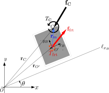
For brevity, the superscript to indicate the coordinate frame is omitted whenever it does not cause any confusion. Applying the Newton’s second law of motion in the reference frame

$$m\ddot{\bf r}_{\text{O}^{\prime}}={\bf f}_{\text{C}}+{\bf f}_{\text{frt}}={\bf f}_{\text{total}}$$ (4)

where $m$ is the mass of the object, $\ddot{(\cdot)}=d^{2}(\cdot)/dt^{2}$, $t$ is time in seconds, and ${\bf f}_{\text{frt}}$ is the sum of all unknown forces including frictional forces. The equation of motion for the rotation is

$$I\ddot{\theta}=T_{\text{C}}+T_{\text{frt}}+{\bf r}_{m}\times{\bf f}_{\text{C}}=T_{\text{total}}$$ (5)

where $I$ is the moment of inertia of the object, ${\bf r}_{m}$ is the distance from the centre of the object to the contact point, which is difference between the tip position, ${\bf r}_{\text{C}}$, and the object centre position, ${\bf r}_{\text{O}^{\prime}}$, i.e., ${\bf r}_{\text{C}}-{\bf r}_{\text{O}^{\prime}}$, and $T_{\text{frt}}$ is the sum of all unknown torque including frictional torques.

To calculate the total sum of forces, ${\bf f}_{\text{total}}$, and the total sum of torques, $T_{\text{total}}$, which are not directly measured or provided in the data set, a PID (Proportional-Integral-Derivative) controller is designed for each to track the measured object position, ${\bf r}_{\text{O}^{\prime}}$, or the measured object orientation, $\theta$ as follows:

$$m\ddot{\bf r}_{\text{sim}} =k_{p}{\bf e}_{r}+k_{i}\int_{0}^{t}{\bf e}_{r}(\tau)d\tau+k_{d}\dot{\bf e}_{s}=\hat{\bf f}_{\text{sim}}$$ (6a)

$$I\ddot{\theta}_{\text{sim}} =l_{p}{e}_{\theta}+l_{i}\int_{0}^{t}{e}_{\theta}(\tau)d\tau+l_{d}\dot{e}_{\theta}=\hat{T}_{\text{sim}}$$ (6b)

where $k_{p}$, $k_{i}$ and $k_{d}$ are the PID gains for the linear motion, $l_{p}$, $l_{i}$, and $l_{d}$ are the PID gains for the rotational motion, and

$${\bf e}_{r} ={\bf r}_{\text{O}^{\prime}}-{\bf r}_{\text{sim}}$$ (7a)

$${e}_{\theta} ={\theta}-{\theta}_{\text{sim}}$$ (7b)

The following set of the control gains are found by trial and error:

Figure 3: Disturbance observer diagram: two inputs to the observer are the measured position or orientation of the object and the force or torque applied by the pusher.

$$k_{p} =46.6,~{}k_{i}=34.6,~{}k_{d}=15.4$$ (8a)

$$l_{p} =117.2,~{}l_{i}=137.8,~{}l_{d}=24.5$$ (8b)

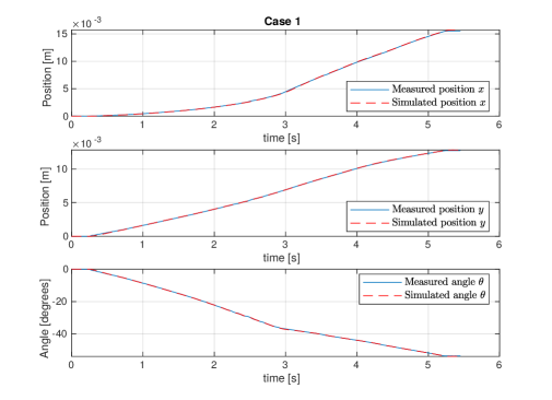
To verify the estimated force and torques, set ${\bf f}_{\text{total}}=\hat{\bf f}_{\text{sim}}$ and $T_{\text{total}}=\hat{T}_{\text{sim}}$ and solve (4) and (5). The position and the orientation calculated using the estimated forces/torques are compared with the measured position and orientation in Figure 2 for Case 1. All trajectories are reasonably close to the measured values. Now, the unknown force and the torque are calculated by

$${\bf f}_{\text{frt}} \approx\hat{\bf f}_{\text{sim}}-{\bf f}_{\text{C}}$$ (9a)

$${T}_{\text{frt}} \approx\hat{T}_{\text{sim}}-{T}_{\text{C}}$$ (9b)

Although this approach provides relatively accurate force and torque estimations, the errors in the estimation are strongly dependent on the choice of PID control gains. It would be very difficult to find appropriate gains working for various push scenarios. Hence, more reliable disturbance estimation algorithm is required. The calculated unknown force and torque by the PID controller are to be used to confirm the performance of disturbance observers to be designed in the next section.

III Algorithm

In this section, firstly, estimating unknown forces or torques in pushing object in a planner surface is posed as a disturbance observer problem. Secondly, a disturbance observer is designed and the performance of the observer is demonstrated using the push data. Finally, a prediction algorithm is designed based on the pattern found in the estimated disturbances.

Figure 4: Force & torque estimation by the disturbance observer. The estimated disturbances are closely matched with the ones from the dynamics simulations.

III-A Disturbance Observer

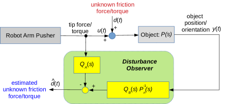
The Q-filter based disturbance observer is shown in Figure 3. The estimated total sum of the disturbances, $\hat{d}(t)$, is given by

$$\hat{d}(t)=-Q_{A}(s)u(t)+Q_{B}(s)P^{-1}_{n}(s)y(t)$$ (10)

where the Laplace domain, $s$, and the time domain, $t$, are used at the same time for a notational convenience, $u(t)$ is the pusher force or torque applied to the object, $y(t)$ is the object position or orientation measurements, and $Q_{A}(s)$, $Q_{B}(s)$ and $P_{n}(s)$ are the transfer functions to be designed. Two inputs to the observer, $u(t)$ and $y(t)$ include some measurement noise, which should be appropriately taken into account when the observer is designed.

If there is no sensor noise and the system transfer function, $P(s)$ is perfectly known, then $y(t)$ is equal to $P(s)[u(t)+d(t)]$. Set $P_{n}(s)=P(s)$ and $Q_{A}(s)=Q_{B}(s)$,

$$\hat{d}(t)=Q_{A}(s)d(t)$$ (11)

Hence, the estimated disturbance, $\hat{d}(t)$, is equal to the external disturbance filtered by $Q_{A}(s)$. For the translational and the rotational dynamics, (4) and (5), the system is a simply double integrator with the inertia, i.e., $P(s)=1/(ms^{2})$ or $P(s)=1/(Is^{2})$. Only uncertain parameter for each is the inertia parameter, mass or the moment of inertia. Mismatch between the known values and the true values can be written as

$$m=\bar{m}+\Delta m,~{}I=\bar{I}+\Delta I$$ (12)

where $\bar{m}$ and $\bar{I}$ are the nominal values, and $\Delta m$ and $\Delta I$ are the uncertainties. As $P_{n}(s)=1/(\bar{m}s^{2})$ or $P_{n}(s)=1/(\bar{I}s^{2})$, the estimated disturbance is given by

$$\hat{d}(t)=\alpha Q_{A}(s)d(t)+(1-\alpha)Q_{A}(s)u(t)$$ (13)

where $\alpha$, equal to $\bar{m}/m$ or $\bar{I}/I$, is strictly positive and becomes 1 for no uncertainty in the inertia properties. For all experimental cases chosen in Table I, $\bar{m}$ is set to 1.045 kg and $\bar{I}$ is equal to 0.0018 kg$\cdot$m² as they are given in [8]. The uncertainties for the inertia properties are presumed to be very small for all the cases.

Figure 5: The linear relationship between the measured force or torque and the estimated force or torque for (a) $x$-direction, (b) $y$-direction and (c) $\theta$-rotation.

$Q_{A}(s)$ and $Q_{B}(s)$ is set to the following form:

$$Q_{A}(s)=Q_{B}(s)=\dfrac{\omega_{n}^{2}}{s^{2}+2\zeta\omega_{n}s+\omega_{n}^{2}}$$ (14)

where $\zeta$ is equal to $1/\sqrt{2}$ and $\omega_{n}$ is equal to 300 rad/s. The value of $\zeta$ is chosen to minimise the settling time, which is important in estimating unknown disturbances having possibly some discontinuous jumps from time to time. While the larger the value for $\omega_{n}$ covers the wider range of frequencies for the disturbances, it would be sensitive to high frequency noises.

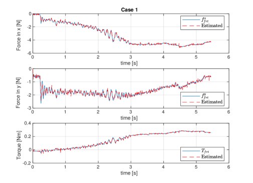
As shown in Figure 4, the disturbance observer estimates the unknown force or torque with very little differences from the ones calculated using the dynamic simulations with the PID controller. It is worth to emphasise that the disturbance observer estimates the total sum of the unknown forces or torques no matter what causes the differences. The observer estimates current disturbances and cannot provide future disturbances. The estimated disturbance cannot be used directly to predict a future trajectory of an object and additional algorithm is required to predict future position and orientation of an object.

III-B Prediction Algorithm

In order to use the estimated disturbances in predicting future position and orientation of an object, a persistent pattern in estimated disturbances must be identified. Once the pattern is identified, future unknown forces would be predicted.

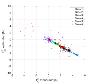
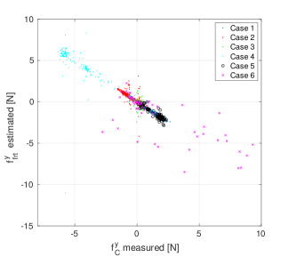
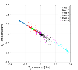
As shown in Figure 5, there are clear linear relationships between the applied force or torque by the robot tip and the estimated unknown disturbances by the observer. These linear relationships remain approximately the same for all six test cases. The acceleration of the object seems to break the linearity as the data points in the figures are spread away from the major cluster for the higher acceleration experiments, i.e., Case 5 and 6. This linear relationship can be written as

$$\hat{d}(t_{k})=\beta u(t_{k})+\epsilon$$ (15)

where $t_{k}\in[t_{1},t_{N}]$ for $k=1,2,3,\ldots,N-1,N$, $N$ is the number of samples during an identification interval between $t_{1}$ and $t_{N}$, $t_{1}$ and $t_{N}$ are the start and the end time of the identification interval, respectively, $\hat{d}(t_{k})$ is the estimated value of ${f}^{x}_{\text{frt}}$, ${f}^{y}_{\text{frt}}$ or $T_{\text{frt}}$ at time $t_{k}$ by the disturbance observer, $u(t_{k})$ is the measured value of $f^{x}_{\text{C}}$, ${f}^{y}_{\text{C}}$ or $T_{\text{C}}$ at time $t_{k}$, and $\beta$ and $\epsilon$ are unknowns to be determined.

Identification phase: the first part of the prediction algorithm is finding the linear relationship. A recursive least-square algorithm is used to determine $\beta$ and $\epsilon$ as follows [10]:

• Initialise: define the following using the current measurements and the current disturbance estimation for $t_{k}\in[t_{1},t_{N}]$:

  $${\bf u} =\begin{bmatrix}u(t_{1})&u(t_{2})&\ldots&u(t_{N})\end{bmatrix}^{T},$$ (16a)

  $${\bf d} =\begin{bmatrix}\hat{d}(t_{1})&\hat{d}(t_{2})&\ldots&\hat{d}(t_{N})\end{bmatrix}^{T},$$ (16b)

  where $(\cdot)^{T}$ is the transpose, and calculate the following:

  $$H_{k} =\begin{bmatrix}{\bf u}&{\bf 1_{N}}\end{bmatrix},P_{k}^{-1}=H_{k}^{T}H_{k},$$ (17a)

  $${\bf x}_{k} =(P_{k}H_{k}^{T})\hat{\bf d},$$ (17b)

  where ${\bf 1}_{N}$ is the N$\times$1 vector whose elements are all 1, ${\bf x}_{k}=[\hat{\beta}_{k}~{}\hat{\epsilon}_{k}]^{T}$, and $\hat{\beta}_{k}$ and $\hat{\epsilon}_{k}$ are the current estimation of $\beta$ and $\epsilon$, respectively.

• Update: construct $\bf{u}$ and ${\bf d}$ using new measurement and estimation sets from another identification time interval, $t_{k}\in[t^{\prime}_{1},t^{\prime}_{N}]$ and update each as follows:

  $$H_{k+1} =\begin{bmatrix}{\bf u}&{\bf 1}_{N}\end{bmatrix},$$ (18a)

  $$P_{k+1}^{-1} =P_{k}^{-1}+H_{k+1}^{T}H_{k+1},$$ (18b)

  $$K_{k+1} =P_{k+1}H_{k+1}^{T},$$ (18c)

  $${\bf x}_{k+1} ={\bf x}_{k}+K_{k+1}\left({\bf d}-H_{k+1}{\bf x}_{k}\right)$$ (18d)

• Re-Initialise:

  $$P_{k}^{-1} =P_{k+1}^{-1}$$ (19a)

  $${\bf x}_{k} ={\bf x}_{k+1}$$ (19b)

  When new measurement and estimation sets are available, go to Update phase and repeat the calculations.
  

Figure 6: Prediction algorithm switching between the identification phase & the prediction phase: the external disturbance (red dashed lines) is estimated during the identification phase. For a demonstration purpose, the tip force (blue line) is sparsely sampled, 10Hz, for the prediction phase and it is treated as a force planning (pink lines) provided by a presumably high-level mission planner.

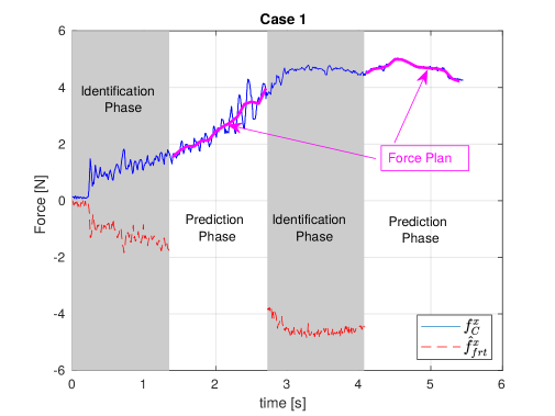
Prediction Phase: the second part of the prediction algorithm is predicting the position and the orientation of object using $\hat{\beta}_{k}$ and $\hat{\epsilon}_{k}$ found in the identification phase To use the MCube Lab push data, the total time of the measurements are divided into four equal time intervals for each scenario as shown in Figure 6. The identification phase and the prediction phase are activated alternatively as shown in the figure. To avoid using the same measured force as a planned force in the prediction phase, where two forces might different in general, a sampled force of the measured with the frequency 10Hz, i.e., a lot sparser force command than the actual measurements, is assumed as the planned force given by a mission planner. Predictions of the position and the orientation are obtained by solving the following differential equations:

$$m\ddot{\bf r}_{\text{O}^{\prime}} ={\bf f}_{\text{plan}}+\text{diag}[\hat{\boldsymbol{\beta}}_{f}]{\bf f}_{\text{plan}}+\hat{\boldsymbol{\epsilon}}_{f}$$ (20a)

$$I\ddot{\theta} =T_{\text{plan}}+\hat{\beta}_{T}T_{\text{plan}}+\hat{\epsilon}_{T}$$ (20b)

where

$${\bf f}_{\text{plan}} ={\bf f}_{C}(t_{k}),$$ (21a)

$$T_{\text{plan}} =T_{\text{C}}(t_{k})+{\bf r}_{m}(t_{k})\times{\bf f}_{\text{C}}(t_{k}),$$ (21b)

$$\text{diag}[\hat{\boldsymbol{\beta}}_{f}] =\begin{bmatrix}\hat{\beta}_{fx}&0\\ 0&\hat{\beta}_{fy}\end{bmatrix},~{}\hat{\boldsymbol{\epsilon}}_{f}=\begin{bmatrix}\hat{\epsilon}_{fx}&\hat{\epsilon}_{fy}\end{bmatrix}^{T},$$ (21c)

$\hat{\beta}_{fx}$ and $\hat{\epsilon}_{fx}$ are the estimated values by the least-square algorithm for $x$-directional motions using the data collected during the identification phase, similarly, $\hat{\beta}_{fy}$, $\hat{\epsilon}_{fy}$, $\hat{\beta}_{T}$, and $\hat{\epsilon}_{T}$ are defined, the initial position and orientation are set to equal to the last measurements in the previous identification phase, and the initial velocity and angular velocity are set to zero as they are not measured directly.

Figure 7: Average and standard deviation of the prediction errors for the proposed algorithm and the simple algorithm

Implementation: it is important to implement the disturbance observer in Figure 3 with $Q_{A}$ given in (14) in the state-space form. The prediction algorithm presented switches between the identification phase and the prediction phase instantaneously. Without a proper initialisation of the internal state of the disturbance observer would cause unnecessary impulse-like peak correction at switching instances.

Simple Algorithm: The proposed prediction algorithm is compared with a simple correction algorithm, which uses a simple friction model as follows:

$$m\ddot{\bf r}_{\text{O'}} ={\bf f}_{\text{plan}}+\mu mg$$ (22a)

$$I\ddot{\theta} =T_{\text{plan}}$$ (22b)

where $\mu$ is the friction coefficient, where the average value of the surface (abs), 0.14, is used, $g$ is the gravitation acceleration, 9.81 m/s². Note that the rotational motion does not have any correction term as it is not clear how to include a simple friction in the rotational motion.

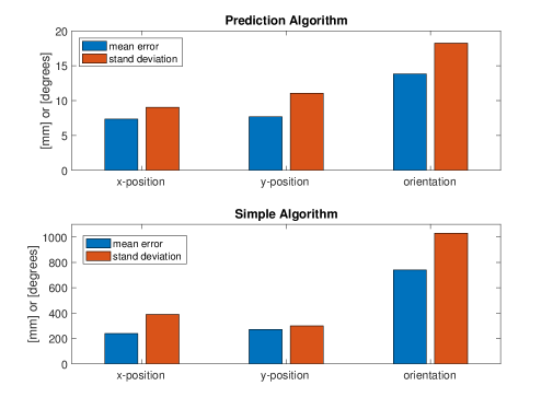
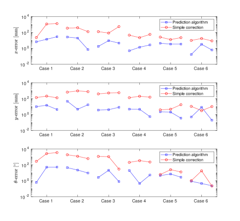
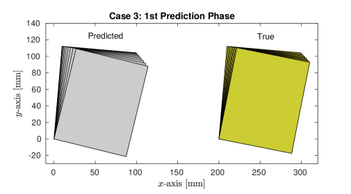
Algorithm Performance: The proposed prediction algorithm is tested for all six scenarios. The average error and the standard deviation for each prediction algorithm are shown in Figure 7. Compare to the simple correction, the average errors for the prediction algorithm are less than 10-fold smaller, restricted well below 10 mm in the $x$ and $y$ positions and 20^∘ in the orientation. The magnitude of error grows as the prediction horizon becomes longer. The main reason that the errors for Case 3, 4, 5 and 6 are relatively smaller than Case 1 and 2 as shown in Figure 8 is their prediction horizons are shorter than the ones for Case 1 and 2 . The best one is the first prediction horizon for Case 3. Its object prediction is compared with the true in Figure 9.

Figure 8: Prediction errors for all three prediction phases for each algorithm

IV Discussions & Future work

The position and orientation prediction algorithm for an object pushed by a robot in a planar surface is developed. The total sum of unknown disturbances is estimated by a disturbance observer and a recurrent least-square algorithm estimates the correlation between the measured force or torque by a sensor attached to the robot arm and the estimated disturbances by the observer. The correlation model, then, is used to predict the unmodelled disturbance corresponding to a planned force or torque given by a high-level mission planning algorithm. Finally, the position and the orientation of the object are predicted. The performance of the algorithm is demonstrated using the push data.

The linear correlation is not, in fact, surprising for constant velocity motions as the force sum must be zero. The relations could be a lot complex for non-zero or varying acceleration cases should considering multiple characteristics of push motions. For adapting to complex situations, machine vision information could be used with the machine learning algorithms as in [3]. Also, instead of predicting a single trajectory, an ensemble of trajectories distribution described by a probability density function would be predicted using nonlinear estimation algorithms such as the particle filter [11] or the nonlinear projection filter [12]. There is also possibility to plan the robot tip movements better for the identification phase in order to maximise information extraction about various physical properties of object, surface, stochastic characteristics, etc.

Figure 9: Best prediction case comparison

References

- [1] M. Bauza and A. Rodriguez, “A probabilistic data-driven model for planar pushing,” in 2017 IEEE International Conference on Robotics and Automation (ICRA), May 2017, pp. 3008–3015.
- [2] N. Fazeli, R. Kolbert, R. Tedrake, and A. Rodriguez, “Parameter and contact force estimation of planar rigid-bodies undergoing frictional contact,” The International Journal of Robotics Research, vol. 36, no. 13-14, pp. 1437–1454, 2017. [Online]. Available: https://doi.org/10.1177/0278364917698749
- [3] A. Kloss, S. Schaal, and J. Bohg, “Combining learned and analytical models for predicting action effects,” CoRR, vol. abs/1710.04102, 2017.
- [4] K.-T. Yu and A. Rodriguez, “Realtime state estimation with tactile and visual sensing. application to planar manipulation,” 2018 IEEE International Conference on Robotics and Automation (ICRA), pp. 7778–7785, 2018.
- [5] W. Chen, J. Yang, L. Guo, and S. Li, “Disturbance-observer-based control and related methods—an overview,” IEEE Transactions on Industrial Electronics, vol. 63, no. 2, pp. 1083–1095, Feb 2016.
- [6] K. Ohishi, M. Nakao, K. Ohnishi, and K. Miyachi, “Microprocessor-controlled dc motor for load-insensitive position servo system,” IEEE Transactions on Industrial Electronics, vol. IE-34, no. 1, pp. 44–49, Feb 1987.
- [7] H. Shim, G. Park, Y. Joo, J. Back, and N. H. Jo, “Yet another tutorial of disturbance observer: robust stabilization and recovery of nominal performance,” Control Theory and Technology, vol. 14, no. 3, pp. 237–249, Aug 2016. [Online]. Available: https://doi.org/10.1007/s11768-016-6006-9
- [8] “The MCube lab - push dataset,” https://mcube.mit.edu/push-dataset/index.html, accessed: 13th March 2019.
- [9] K. Yu, M. Bauzá, N. Fazeli, and A. Rodriguez, “More than a million ways to be pushed: A high-fidelity experimental data set of planar pushing,” CoRR, vol. abs/1604.04038, 2016. [Online]. Available: http://arxiv.org/abs/1604.04038
- [10] J. L. Crassidis and J. L. Junkins, Optimal Estimation of Dynamic Systems, 2nd ed. New York, NY, the USA: Chapman and Hall/CRC, 2011, pp.19-25.
- [11] M. S. Arulampalam, S. Maskell, N. Gordon, and T. Clapp, “A tutorial on particle filters for online nonlinear/non-gaussian bayesian tracking,” IEEE Transactions on Signal Processing, vol. 50, no. 2, pp. 174–188, Feb 2002.
- [12] J. Kim and R. Richardson, “Negative-free approximation of probability density function for nonlinear projection filter,” in 2016 IEEE 55th Conference on Decision and Control (CDC), Dec 2016, pp. 3738–3743.