The quantum cost function concentration dependency
on the parametrization expressivity
Abstract
Although we are currently in the era of noisy intermediate scale quantum devices, several studies are being conducted with the aim of bringing machine learning to the quantum domain. Currently, quantum variational circuits are one of the main strategies used to build such models. However, despite its widespread use, we still do not know what are the minimum resources needed to create a quantum machine learning model. In this article, we analyze how the expressiveness of the parametrization affects the cost function. We analytically show that the more expressive the parametrization is, the more the cost function will tend to concentrate around a value that depends both on the chosen observable and on the number of qubits used. For this, we initially obtain a relationship between the expressiveness of the parametrization and the mean value of the cost function. Afterwards, we relate the expressivity of the parametrization with the variance of the cost function. Finally, we show some numerical simulation results that confirm our theoretical-analytical predictions.
I Introduction
In recent years, there has been a great increase in interest in quantum computing due to its possible applications in solving problems such as simulation of quantum systems quantum_simulation , development of new drugs drug_discovery , and resolution of systems of equations linear linear_system . Quantum machine learning, which is an interdisciplinary area of study between machine learning and quantum computing, is also another possible application that should benefit from the computational power of these devices. In this sense, several models have already been proposed, such as Quantum Multilayer Perceptron quantum_model_multilayer_perception , Quantum Convolutional Neural Networks qunatum_Convolutional , Quantum Kernel Method kernel_methods , and Quantum-Classical Hybrid Neural Networks hybrid_1 ; hybrid_2 ; hybrid_3 ; hybrid_4 . However, in the era of noisy intermediate scale quantum devices (NISQ), variational quantum algorithms (VQAs) VQA are the main strategy used to build such models.
Variational quantum algorithms are models that use a classical optimizer to minimize a cost function by optimizing the parameters of a parametrization . Several optimization strategies have already been proposed Friedrich_es ; Anand ; Zhou_leo ; fosel_thomas , although this is an open area of study. In fact, despite the widespread use of VQAs, our understanding of VQAs is limited and some problems still need to be solved, such as the disappearance of the gradient McClean ; BR_cost_Dependent ; BR_Entanglement_devised_barren_plateau_mitigation ; BR_Entanglement_induced_barren_plateaus ; BR_expressibility ; BR_noise ; BR_gradientFree , methods to mitigate the Barren Plateaus issue FRIEDRICH ; BR_initialization_strategy ; BR_Large_gradients_via_correlation ; BR_LSTM ; BR_layer_by_layer , how to build a parameterization Quantum_architecture_Kuo ; Friedrich_Restricting , and how correct errors Quantum_error_mitigation .
In this sense, in this article we aim to analyze how the expressivity of the parametrization affects the cost function. We will show that the more expressive the parametrization is, the more the average value of the cost function will concentrate around a fixed value. In addition, we will also show that the probability of the cost function deviating from its average will also depend on the quantum circuit expressivity.
The remainder of this article is organized as follows. In Section II, we make a short introduction about VQAs. In Section III, we comment on how expressiveness can be quantified and what is its meaning. In the following section, Section IV, we present our main results. There we will give two theorems. In Theorem 1, we obtain a relationship between the concentration of the cost function and the expressiveness of the parametrization. In Theorem 2, we obtain the probability for the cost function to deviate from its average value, restricting it via a function of the quantum circuit expressivity. Then, in Section V, we present some numerical simulation results to confirm our theoretical analytical predictions. Finally, Section VI presents our conclusions.
II Variational quantum algorithms
Variational quantum algorithms are models where a classical optimizer is used to minimize a cost function, which is usually written as the average value of an observable :
| (1) |
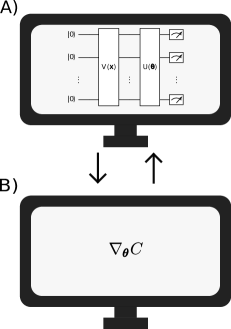
where . To do so, the optimizer updates the parameters of the parameterization . In Fig. 1, one can see a schematic representation of how a VQA works. In the first part, Fig. 1 A, a quantum circuit runs on a quantum computer. In general, this circuit is divided into three parts. In the first part we have a parametrization that is used to encode data in a quantum state. In quantum machine learning, this parametrization is used to bring our data, such as data from the MNIST mnist_dataset dataset, into a quantum state. Next, we have the parametrization that will depend on the parameters that we must optimize. Finally, we have the measures that are used to calculate the cost function. In the second part, Fig. 1 B, we have a classical computer that performs the task of optimizing the parametrization parameters. In general, for this task the gradient of the cost function is used.
In this article, the parametrization will be given by
| (2) |
where is the number of layers, is a layer that depends on the parameters and is a layer that does not depend on the parameters . The construction of parametrizations is still an open area of study and, due to the complexity involved in its construction, some works have proposed using the automation of this process Quantum_architecture_Kuo ; Zhang_Shi_Xin . Furthermore, for problems such as quantum machine learning, where a parameterization is used to encode data in a quantum state, the choice of is also extremely important Schuld_data , and several possible encoding forms have been proposed LaRose_Ryan .
III Expressivity
Following Ref. Sim_Expressibility , here we define expressivity as the ability of a quantum circuit to generate (pure) states that are well representative of the Hilbert space. In the case of a qubit, this comes down to the quantum circuit’s ability to explore the Bloch sphere. To quantify the expressiveness of a quantum circuit, we can compare the uniform distribution of units obtained from the set with the maximally expressive (Haar) uniform distribution of units of . For this, we use the following super-operator BR_expressibility
| (3) |
where is a volume element of the Haar measure and is a volume element corresponding to the uniform distribution over . The uniform distribution over is obtained by fixing the parameterization , where for each vector of parameters we obtain a unit . Thus, given the set of parameters , we obtain the corresponding set of unitary operators:
| (4) |
IV Main Theorems
In this section, we present our main results. First, we obtain a relationship between the average value of the cost function, Eq. (1), with the expressivity of the parametrization , Eq. (2). Afterwards, we will obtain a relationship between the variance of the cost function and the expressiveness of the parametrization. To do so, we start by writing the average of the cost function as
| (5) |
Therefore, using Eq. (3) in Eq. (5), we obtain the following relationship between the mean of the cost function and the expressivity of the parametrization, Theorem 1.
Theorem 1
The proof of this theorem is presented in Appendix A.
Above we used the matrix -norm . For any operator , from Eq. (3), we have that the smaller , with , the more expressive will be the parametrization. Therefore, Theorem 1 implies that the greater the expressiveness of the parameterization , the more the cost function average will tend to have the value .
Despite Theorem 1 implying a tendency of the mean value of the cost function to go a fixed value, when executing the VQA, the cost function may deviate from its mean. To calculate this deviation we use the Chebyshev inequality,
| (7) |
which informs the probability for the cost function to deviate from its mean value.
Next, we present the Theorem 2, relating the modulus of the cost function variance with the expressiveness of the parametrization.
Theorem 2
The proof of this theorem is presented in Appendix B.
As the variance is a positive real number, we can use Theorem 2 to analyze the probability that the cost function deviates from its mean, Eq. (7). Therefore, from Theorem 2, we see that by defining the observable and the size of the system, that is, the number of qubits used, the probability of the cost function deviating from its mean decreases as the expressivity increases. Furthermore, it also follows, from Theorem 1, that for maximally expressive parameterizations, i.e., for , the cost function will be stuck to the fixed value .
V Simulation Results
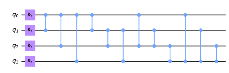
In this section we will present some numerical simulation results. For this, we use twelve different parametrizations, which we call, respectively, Model 1, Model 2, …, Model 12. See Appendix C for the corresponding quantum circuits. As we saw in Eq. (2), the parametrization is obtained from the product of layers , where each layer can be distinct from one another, that is, the gates and sequences we use in one layer may be different from another. However, in general, they are the same. For the results shown here, the layers are the same, the only difference being the parameters used in each layer.
For these results we define each as
| (11) |
where the index indicates the layer and the index the qubit. Also, we use in all models. In the parametrizations of Model 3, Model 4, Model 6, Model 9, Model 10, and Model 12, Figs. 10, 11, 13, 16, 17, and 19, respectively, before for each , we apply the Hadamard gate to all the qubits. Furthermore, in Model 2, Model 3, Model 8, and Model 9, Figs. 9, 10, 15, and 16, respectively, we use the controlled port , or . Finally, for the results obtained here, we used the PennyLane Pennylane_bibli library. Furthermore, the codes used to obtain these results are available for access in https://github.com/lucasfriedrich97/quantum-expressibility-vs-cost-function.
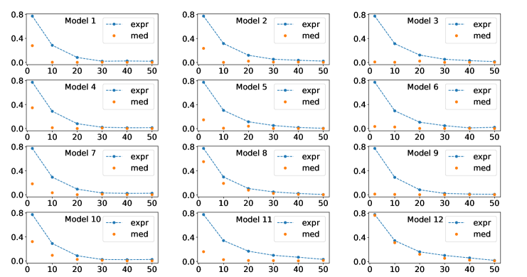
Initially, we numerically analyze Eq. (6) of Theorem 1. For this, we performed an initial set of simulations, Figs. 2, 3, and 4, where we fixed the number of qubits and varied the number of layers . For the results of Figs. 2, 3, and 4, we used four, five, and six qubits, respectively. Furthermore, for these simulations we consider the particular case and .
Initially, we analytically calculate the value of , where we get BR_expressibility
| (12) |
with
| (13) |
Or, from Ref. Sim_Expressibility , we obtain
| (14) |
So, to calculate we generated 5000 pairs of state vectors. Although we have generated a large number of state vectors, it is still a small sample of the entire Hilbert space. So, the value we obtained for is an approximation. As a consequence, in some simulations we obtained a complex value for , Eq. (12). Therefore, whenever this occurred, we restarted the simulation. Furthermore, we also used 5000 units to average the cost function.
In Figs. 2, 3, and 4 is shown the behavour of the right hand side of Eq. (6), related to the expressivity, and of the average cost function term, the left hand side of Eq. (6). For producing these figures, four, five, and six qubits quantum circuits were used, respectively.
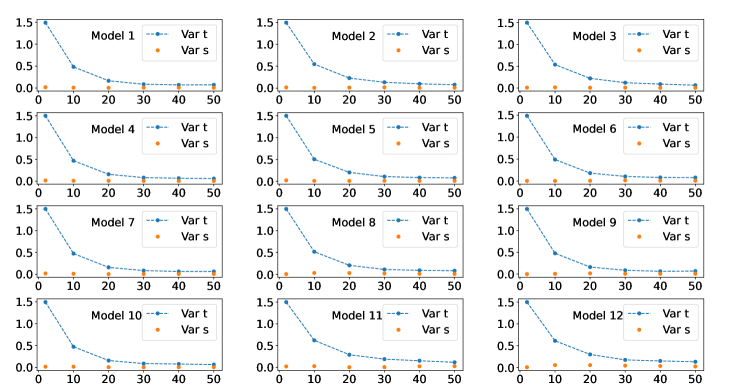
In Figs. 5, 6, and 7, we show the behavior of the numerically calculated variance, Var s, the left hand side of Eq. (8), and of the theoretical value, Var t, the right hand side of Eq. (8), where we again used four, five, and six qubits, respectively. Also, we again used 5000 unitaries to compute the averages.


VI Conclusion
In this article, we analyzed how the expressiveness of the parametrization affects the cost function. As we observed, the concentration of the average value of the cost function has an upper limit that depends on the expressiveness of the parametrization, where, the more expressive this parametrization is, the more the average of the cost function will be concentrated around the fixed value , Theorem 1. Furthermore, the probability for the cost function to deviate from its mean also depends on the expressiveness of the parametrization, Theorem 2.
A possible implication of these results is related to the training of VQAs with highly expressive parametrizations. Once the more expressive the parametrization is, the more the average value of the cost function will be concentrated around , and the probability of the cost function deviating from this average also decreases, considering that, for the case where , the cost function will be stuck at the value . This result is in agreement with the one obtained in Ref. BR_expressibility , where it was shown that the phenomenon of gradient disappearance is related with parametrization having high expressivity.
Another possible implication of our results is related to quantum machine learning models. In Ref. Hubregtsen_Thomas , the authors mentioned that there is a correlation between expressiveness and accuracy, where the greater is the expressiveness, in general, the greater is the accuracy. To this end, the authors used Person’s correlation coefficient to quantify this correlation. However, our results imply that, not only is the training of highly expressive parametrized quantum machine learning models difficult, as it will suffer more from the problem of gradient disappearance, as indicated in Ref. BR_expressibility , but also the cost function itself will become stuck to a region close to the value .
Acknowledgements.
This work was supported by the National Institute for the Science and Technology of Quantum Information (INCT-IQ), process 465469/2014-0, and by the National Council for Scientific and Technological Development (CNPq), processes 309862/2021-3 and 409673/2022-6.References
- (1) S. Lloyd, Universal quantum simulators, Science 273, 1073 (1996).
- (2) Y. Cao, J. Romero, and A. Aspuru-Guzik, Potential of quantum computing for drug discovery, IBM Journal of Research and Development 62, 6 (2018).
- (3) A. W. Harrow, A. Hassidim, and S. Lloyd, Quantum algorithm for linear systems of equations, Phys. Rev. Lett. 103, 150502 (2009).
- (4) C. Shao, A quantum model for multilayer perceptron, arXiv.1808.10561 (2018).
- (5) S. J. Wei, Y. H. Chen, Z. R. Zhou, and G. L. Long, A quantum convolutional neural network on NISQ devices, AAPPS Bull. 32, 2 (2022).
- (6) M. Schuld, Supervised quantum machine learning models are kernel methods, arXiv.2101.11020 (2021).
- (7) J. Liu et al., Hybrid quantum-classical convolutional neural networks, Sci. China Phys. Mech. Astron. 64, 290311 (2021).
- (8) Y. Liang, W. Peng, Z.-J. Zheng, O. Silvén, and G. Zhao, A hybrid quantum–classical neural network with deep residual learning, Neural Networks 143, 133 (2021).
- (9) R. Xia and S. Kais, Hybrid quantum-classical neural network for calculating ground state energies of molecules, Entropy 22, 828 (2020).
- (10) E. H. Houssein, Z. Abohashima, M. Elhoseny, and W. M. Mohamed, Hybrid quantum convolutional neural networks model for COVID-19 prediction using chest X-Ray images, Journal of Computational Design and Engineering 9, 343 (2022).
- (11) M. Cerezo et al., Variational quantum algorithms, Nature Rev. Phys. 3, 625 (2021).
- (12) L. Friedrich and J. Maziero. Natural evolutionary strategies applied to quantum-classical hybrid neural networks, arXiv preprint arXiv:2205.08059 (2022).
- (13) A. Anand, M. Degroote, and A. Aspuru-Guzik, Natural evolutionary strategies for variational quantum computation, Mach. Learn.: Sci. Technol. 2, 045012 (2021).
- (14) L. Zhou et al., Quantum approximate optimization algorithm: Performance, mechanism, and implementation on near-term devices, Phys. Rev. X 10, 021067 (2020).
- (15) T. Fösel et al., Quantum circuit optimization with deep reinforcement learning, arXiv preprint arXiv:2103.07585 (2021).
- (16) J. R. McClean et al., Barren plateaus in quantum neural network training landscapes, Nature Comm. 9, 4812 (2018).
- (17) M. Cerezo, A. Sone, T. Volkoff, L. Cincio, and P. J. Coles, Cost function dependent barren plateaus in shallow parametrized quantum circuits, Nature Comm. 12, 1791 (2021).
- (18) T. L. Patti, K. Najafi, X. Gao, and S. F. Yelin, Entanglement devised barren plateau mitigation, Phys. Rev. Research 3, 033090 (2021).
- (19) C. O. Marrero, M. Kieferová, and N. Wiebe, Entanglement-induced barren plateaus, PRX Quantum 2, 040316 (2021).
- (20) Z. Holmes, K. Sharma, M. Cerezo, and P. J. Coles, Connecting ansatz expressibility to gradient magnitudes and barren plateaus, PRX Quantum 3, 010313 (2022).
- (21) S. Wang et al., Noise-induced barren plateaus in variational quantum algorithms, Nature Commu. 12, 6961 (2021).
- (22) A. Arrasmith, M. Cerezo, P. Czarnik, L. Cincio, and P. J. Coles, Effect of barren plateaus on gradient-free optimization, Quantum 5, 558 (2021).
- (23) L. Friedrich and J. Maziero, Avoiding barren plateaus with classical deep neural networks, Phys. Rev. A 106, 042433 (2022).
- (24) E. Grant, L. Wossnig, M. Ostaszewski, and M. Benedetti, An initialization strategy for addressing barren plateaus in parametrized quantum circuits, Quantum 3, 214 (2019).
- (25) T. Volkoff and P. J. Coles, Large gradients via correlation in random parameterized quantum circuits, Quantum Sci. Technol. 6, 025008 (2021).
- (26) G. Verdon et al., Learning to learn with quantum neural networks via classical neural networks, https://doi.org/10.48550/arXiv.1907.05415 (2019).
- (27) A. Skolik, J. R. McClean, M. Mohseni, P. van der Smagt, and M. Leib, Layerwise learning for quantum neural networks, Quantum Mach. Intell. 3, 5 (2021).
- (28) Y. LeCun, The MNIST database of handwritten digits, http://yann.lecun.com/exdb/mnist/ (1998).
- (29) E.-J. Kuo, Y.-L. L. Fang, S. Y.-C. Chen, Quantum architecture search via deep reinforcement learning, arXiv preprint arXiv:2104.07715 (2021).
- (30) L. Friedrich and J. Maziero, Restricting to the chip architecture maintains the quantum neural network accuracy, if the parameterization is a -design, arXiv preprint arXiv:2212.14426 (2022).
- (31) S.-X. Zhang, C.-Y. Hsieh, S. Zhang, and H. Yao, Differentiable quantum architecture search, Quantum Sci. Technol. 7, 045023 (2022).
- (32) Z. Zhenyu et al., Quantum error mitigation, arXiv preprint arXiv:2210.00921 (2022).
- (33) M. Schuld, R. Sweke, and J. J. Meyer, Effect of data encoding on the expressive power of variational quantum-machine-learning models, Phys. Rev. A 103, 032430 (2021).
- (34) R. LaRose and B. Coyle, Robust data encodings for quantum classifiers, Phys. Rev. A 102, 032420 (2020).
- (35) S. Sim, P. D. Johnson, A. Aspuru-Guzik, Expressibility and entangling capability of parameterized quantum circuits for hybrid quantum-classical algorithms, Adv. Quantum Technol. 2, 1900070 (2019).
- (36) V. Bergholm et al., Pennylane: Automatic differentiation of hybrid quantum-classical computations, arXiv preprint arXiv:1811.04968 (2018).
- (37) T. Hubregtsen, J. Pichlmeier, P. Stecher, and K. Bertels, Evaluation of parameterized quantum circuits: on the relation between classification accuracy, expressibility, and entangling capability, Quantum Mach. Intell. 3, 9 (2021).
- (38) B. Collins and P. Śniady, Integration with respect to the Haar measure on unitary, orthogonal and symplectic group, Commun. Math. Phys. 264, 773 (2006).
- (39) Z. Puchała and J. A. Miszczak, Symbolic integration with respect to the Haar measure on the unitary group, Bull. Pol. Acad. Sci.-Tech. Sci. 65, 1 (2017).
Appendix A Proof of Theorem 1
For the proofs we present in this and in the next appendix, we shall need the following lemmas:
Lemma 1
Let form a unitary t-design with , and let be arbitrary linear operators. Then
| (15) |
Lemma 2
Let form a unitary t-design with , and let be arbitrary linear operators. Then
| (16) |
where . For more details on the proofs of these lemmas, see Refs. Harr_measure_1 ; Harr_measure_2 .
We will also use the definition of expressivity given in Eq. (3). For proving Theorem 1, we start by writing the mean of the cost function as in Eq. (5) Using given by Eq. (3) with in Eq. (5), we get
| (17) |
Using the cyclicity of the trace function and Lemma 1, we obtain
| (18) |
where we used that . From Eq. (17), it follows that
| (19) |
Above we used the Cauchy-Schwarz inequality. With this, we have proved Theorem 1.
Appendix B Proof of Theorem 2
In this section, we will prove Theorem 2. To do so, we start by writing the variance as
| (20) |
where has already been obtained in Eq. (17). Therefore, we get , which will be given by
| (21) |
Thus, using in Eq. (21), with , we get
| (22) |
To solve the integral that appears in Eq. (22), we use Lemma 2. So
| (23) |
where we again used the cyclicity of the trace function. We also used and .
Using this result in Eq. (22), we get
| (24) |
Appendix C Appendix C
For all simulations that we presented in Sec. V, we used the parametrizations shown in the figures below.