Generalized Zurek’s bound on the cost of an individual classical or quantum computation

Abstract

We consider the minimal thermodynamic cost of an individual computation, where a single input $x$ is mapped to a single output $y$. In prior work, Zurek proposed that this cost was given by $K(x|y)$, the conditional Kolmogorov complexity of $x$ given $y$ (up to an additive constant which does not depend on $x$ or $y$). However, this result was derived from an informal argument, applied only to deterministic computations, and had an arbitrary dependence on the choice of protocol (via the additive constant). Here we use stochastic thermodynamics to derive a generalized version of Zurek’s bound from a rigorous Hamiltonian formulation. Our bound applies to all quantum and classical processes, whether noisy or deterministic, and it explicitly captures the dependence on the protocol. We show that $K(x|y)$ is a minimal cost of mapping $x$ to $y$ that must be paid using some combination of heat, noise, and protocol complexity, implying a tradeoff between these three resources. Our result is a kind of “algorithmic fluctuation theorem” with implications for the relationship between the Second Law and the Physical Church-Turing thesis.

I Introduction

It is now understood that there are fundamental relationships between computational and thermodynamic properties of physical processes. The best-known relationship is Landauer’s bound, which says that any computational process that erases statistical information must generate a corresponding amount of thermodynamic entropy in its environment (landauer1961irreversibility, ; benn82, ). For concreteness, imagine a process that implements some stochastic input-output map $p(y|x)$ while coupled to a heat bath at inverse temperature $\beta$. Suppose that the process is initialized with some ensemble of inputs $p(x)$ which is mapped to an ensemble of outputs $p(y)=\sum_{x}p(y|x)p(x)$. Landauer’s bound implies that the generated heat, averaged across the ensemble of system trajectories, obeys

$${\textstyle\frac{\beta}{\ln 2}}\langle Q\rangle\geq S(p(X))-S(p(Y)),$$ (1)

where $S(\cdot)$ is the Shannon entropy in bits. The result imposes a minimal “thermodynamic cost of computation”, i.e., a minimal amount of internal energy and/or work that must be lost as heat.

Importantly, Landauer’s bound depends not only on properties of the physical process but also on the choice of the input ensemble $p(x)$. Because of this, it cannot be used to investigate the following natural question: what is the cost of mapping a single input $x$ to a single output $y$, independently of which statistical ensembles (if any) the inputs are drawn from? As a motivating example, imagine a process that deterministically maps the logical state of a 100GB hard drive from some particular sequence of $10^{11}$ zeros-and-ones to a sequence of $10^{11}$ zeros. Without additional assumptions about the input ensemble, one cannot use Landauer’s bound to constrain the heat generated by this process. The same holds for most other bounds on the thermodynamic costs of computation, which typically depend on the choice of the input ensemble (maroney2009generalizing, ; faist2015minimal, ; parrondo2015thermodynamics, ; kolchinsky2016dependence, ; boyd2016identifying, ; ouldridge2017fundamental, ; Boyd:2018aa, ; wolpert2019stochastic, ; wolpert2020thermodynamic, ; riechers2021initial, ; riechersImpossibilityLandauerBound2021, ; kolchinsky2021dependence, ; kardecs2022inclusive, ).

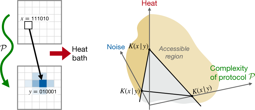
Figure 1: We analyze the cost of mapping a single input $x$ to a single output $y$, given a system coupled to a heat bath and a work reservoir that drives protocol $\mathcal{P}$. We show that the conditional Kolmogorov complexity $K(x|y)$ is a fundamental minimal cost, which bounds accessible combinations of heat, noise, and complexity of the protocol.

In this paper, we derive a lower bound on the heat generated by an individual computation that maps a single input $x$ to a single output $y$ (see 1). Our bound, which appears in Section III below, depends only on the properties of $x$, $y$, and the protocol that carries out the transformation $x\shortrightarrow y$. It reflects the loss of algorithmic information in going from $x$ to $y$ (livi08, ), rather than the loss of statistical information in going from the ensemble $p(x)$ to $p(y)$, as in Landauer’s bound.

To derive our result, we suppose without loss of generality that $x$ and $y$ can be represented by binary strings. The loss of algorithmic information is quantified as the length of the shortest computer program that outputs $x$ when provided with $y$ as input:

$$K(x|y)=\min_{s}\ell(s)\quad\text{such that}\quad\mathfrak{C}(s,y)=x.$$ (2)

Here the minimization is over all binary strings, $\ell(s)$ indicates the length of string $s$, and $\mathfrak{C}(s,y)$ indicates the output of a fixed universal computer $\mathfrak{C}$ on program $s$ and input $y$. In algorithmic information theory, $K(x|y)$ is termed the conditional Kolmogorov complexity of $x$ given $y$ (livi08, ; vitanyi2013conditional, ).

The conditional Kolmogorov complexity quantifies how much information must be added to $y$ in order to recover $x$, and so it can be understood as the amount of algorithmic information about $x$ that is not in $y$. It is the algorithmic analog of conditional entropy in Shannon’s information theory, and it has many remarkable mathematical properties. Since it is defined at the level of individual strings, rather than statistical ensembles like Shannon entropy, it is well-suited for studying the cost of individual computations.

Our approach builds on the work by Zurek from the late 1980s (zure89a, ), which suggested that $K(x|y)$ can be used to bound the cost of an individual computation $x\shortrightarrow y$ without reference to any statistical ensembles (see also (zure89b, ; bennett1993thermodynamics, ; bennett1998information, ; baumeler2019free, )). Zurek considered a system in contact with an environment, such as a heat bath at inverse temperature $\beta$, which maps some input $x$ to output $y$ in a deterministic (noiseless) manner. He argued that the heat generated by the individual computation, which we write as $Q(x\shortrightarrow y)$, obeys

$${\textstyle\frac{\beta}{\ln 2}}Q(x\shortrightarrow y)\geq K(x|y)+O(1),$$ (3)

where $O(1)$ refers to an arbitrary constant that does not depend on $x$ or $y$, but does depend on the choice of the universal computer $\mathfrak{C}$ and the protocol that implements the computation. Zurek’s bound may be compared to Landauer’s bound (1), since the latter can be written as ${\textstyle{\textstyle\frac{\beta}{\ln 2}}}\langle Q\rangle\geq S(p(X|Y))$ in the case where $X$ is a deterministic function of $Y$. The conditional Shannon entropy $S(p(X|Y))$ quantifies the loss of statistical information about the input given the output, averaged across the ensemble of computational trajectories; the conditional Kolmogorov complexity $K(x|y)$ quantifies the loss of algorithmic information about the input given the output at the level of a single computation. Importantly, Zurek’s bound is not simply a special case of Landauer’s bound where the initial ensemble is concentrated on a single input $x$, since in that case $S(p(X|Y))$ vanishes while $K(x|y)$ generally does not.

Zurek’s bound suggests a remarkable connection between thermodynamics and algorithmic information theory. However, it has some drawbacks. First, it is limited to deterministic computations. Second, it is only meaningful when considering the behavior of a fixed protocol on different inputs. In fact, for any particular $x$ and $y$, one can construct a special protocol that computes $x\shortrightarrow y$ while generating an arbitrarily small amount of heat (Sec. V, kolchinsky2020thermodynamic, ). Finally, as we discuss below, Zurek’s bound was derived using an informal argument that invoked Landauer’s bound as an intermediate step. This is problematic because, as mentioned above, Landauer’s bound only applies at the level of statistical ensembles, not individual computations. This suggests that Zurek’s original derivation made an implicit assumption about the statistical distribution of inputs.

Our result is a generalized version of Zurek’s bound that overcomes all of these issues. It holds for classical and quantum processes, noisy as well as deterministic. In addition, it explicitly quantifies how the choice of protocol enters into the bound, via a “protocol complexity” term. Finally, our bound is derived in an explicit manner within a rigorous Hamiltonian framework. Our derivation uses a combination of techniques from algorithmic information theory and stochastic thermodynamics, which together allow us to study the thermodynamic properties of individual computational trajectories. In general, our work contributes to the growing body of recent research on the relationship between algorithmic information theory and nonequilibrium thermodynamics (hiura2019microscopic, ; kolchinsky2020thermodynamic, ; ro2022model, ; wolpert2019stochastic, ; baumeler2019free, ).

Although our result is motivated within the context of the thermodynamics of computation, it is not restricted to systems that are conventionally considered to be computers. In fact, it is a general algorithmic bound on the heat generated by any system that undergoes the transformation $x\shortrightarrow y$ while coupled to a thermal reservoir. For this reason, it may also be used to study the thermodynamic properties of individual instances of other types of processes, including work extraction (rio2011thermodynamic, ; skrzypczyk2014work, ; hovhannisyan2020charging, ) and algorithmic cooling (schulman2005physical, ; allahverdyan2011thermodynamic, ; raeisi2015asymptotic, ) protocols.

Our paper is structured as follows. In the next section, we provide preliminaries and discuss our setup. We derive our main results in III and illustrate it with examples in IV. We relate our approach to prior work in V. A brief discussion follows in VI. Derivations of our bound and its achievability are found in the appendices.

II Preliminaries

II.1 Physical setup

We consider a simple and operationally accessible physical setup, inspired by “two-point measurement” schemes used in quantum thermodynamics (tasaki2000jarzynski, ; esposito2009nonequilibrium, ; campisi2011colloquium, ; manzanoQuantumFluctuationTheorems2018, ; BuscemiBayesianRetrodiction2021, ). We suppose that there is a computational subsystem $A$ which carries out the transformation $x\shortrightarrow y$. This subsystem is coupled to a thermal bath, represented by subsystem $B$. The overall setup may be classical or quantum, though here we focus on the quantum case for generality.

We assume that the Hilbert spaces of $A$ and $B$ are both separable, so that each one can be associated with a countable orthonormal basis. The basis of subsystem $A$ is indexed by some set of binary strings $\mathcal{A}\subseteq\{0,1\}^{*}$, which we indicate as $\{|a\rangle\}_{a\in\mathcal{A}}$. (The notation $\{0,1\}^{*}$ refers to the countable set of binary strings of finite, but arbitrary, length.) The basis vectors $|a\rangle$ represent logical states, so that the computation $x\shortrightarrow y$ corresponds to a physical process during which subsystem $A$ goes from the initial state $|x\rangle$ to the final state $|y\rangle$. The environment $B$ is a heat bath at inverse temperature $\beta$ and Hamiltonian $H_{B}$. We indicate the spectral decomposition of the Hamiltonian as $H_{B}=\sum_{b\in\mathcal{\mathcal{B}}}\epsilon_{b}|b\rangle\langle b|,$ where $\mathcal{B}$ indexes the bath’s energy eigenstates as $\{|b\rangle\}_{b\in\mathcal{B}}$. We indicate the product basis formed by the logical states of $A$ and the energy eigenstates of $B$ as $V=\{|a,b\rangle\}_{a\in\mathcal{A},b\in\mathcal{B}}$.

The computation $x\shortrightarrow y$ is carried out as follows. $A$ and $B$ start in a pure product state $|x,b\rangle\in V$, where $|b\rangle$ is sampled from the Gibbs distribution $\pi(b)=e^{-\beta\epsilon_{b}}/Z$. The two subsystems are then coupled to an external work reservoir and undergo a Hamiltonian driving protocol over time $t\in[0,\tau]$, corresponding to a time-dependent Hamiltonian $H_{AB}(t)$. As a result of this driving protocol, $A$ and $B$ jointly evolve according to the final state $U|x,b\rangle$ under the unitary $U=\mathcal{T}e^{-(i/\hbar)\int_{0}^{\tau}H_{AB}(t)\,dt}$, where $\mathcal{T}$ is the time-ordered exponential. Finally, $A$ and $B$ undergo a projective measurement in the product basis $V$. Given initial state $|x,b\rangle$, the probability of measuring output logical state $|y\rangle$ and bath energy eigenstate $|c\rangle$ is

$$p(y,c|x,b)=|\langle y,c|U|x,b\rangle|^{2}.$$ (4)

We refer to the combination of the product basis $V$, the unitary $U$, the inverse temperature $\beta$, and the bath’s energy function $\epsilon$ as “the protocol $\mathcal{P}=(V,U,\beta,\epsilon)$”.

We will be interested in two properties of the computation $x\shortrightarrow y$ as instantiated by the protocol $\mathcal{P}$. The first property is the conditional probability of output $y$ given input $x$, averaged across bath states:

$$p(y|x)=\sum_{b,c}p(y,c|x,b)\pi(b).$$ (5)

The second property is the heat generated by the computation $x\shortrightarrow y$:

$$Q(x\shortrightarrow y) =\sum_{b,c}\frac{p(y,c|x,b)\pi(b)}{p(y|x)}(\epsilon_{c}-\epsilon_{b}).$$ (6)

This is the average energy increase of the bath, conditioned on input logical state $x$ and output logical state $y$.

II.2 Computability and description of the protocol

In order to derive our results, we make an important computability assumption in regards to the protocol $\mathcal{P}=(V,U,\beta,\epsilon)$: we assume that there exists a program for a universal computer $\mathfrak{C}$ that can approximate, to any desired degree of numerical precision, the values of

$$\beta,\quad\epsilon_{b},\quad p(y,c|x,b) =|\langle y,c|U|x,b\rangle|^{2} x,b,y,c$$ for all . (7)

We discuss the physical meaning of the computability assumption at the end of this paper.

We refer to the shortest program that computes the values (7) as $\mathcal{P}^{*}$. We emphasize that any program that can compute these values can also be used to compute the bath Gibbs distribution $\pi(b)=e^{-\beta\epsilon_{b}}/Z$, as well as the entries of the stochastic input-output map $p(y|x)$ and the generated heat $Q(x\shortrightarrow y)$, via (5) and (6) respectively. Therefore, $\mathcal{P}^{*}$ can be interpreted as the minimal description of the relevant computational and thermodynamic properties of the physical protocol. We refer to the length of this minimal description $\mathcal{P}^{*}$ as “the complexity of protocol $\mathcal{P}$”, and indicate it as $K(\mathcal{P})\equiv\ell(\mathcal{P}^{*})$.

In deriving our results, we will make use of the conditional Kolmogorov complexity $K(x|y)$, as defined in (2). We also make use of the conditional Kolmogorov complexity $K(x|y,\mathcal{P}^{*})$, which is defined in a similar way as the length of the shortest program that outputs $x$ when provided with $y$ and the minimal description $\mathcal{P}^{*}$ as input. $K(x|y,\mathcal{P}^{*})$ quantifies the algorithmic information about $x$ that is not found in the combination of $y$ and $\mathcal{P}^{*}$. It can be related to $K(x|y)$ and $K(\mathcal{P})$ via the inequalities

$$K(x|y) \geq K(x|y,\mathcal{P}^{*})+O(1)$$ (8)

$$K(x|y) \leq K(\mathcal{P})+K(x|y,\mathcal{P}^{*})+O(1),$$

where $O(1)$ refers to additive constants that do not depend on $x$, $y$, or $\mathcal{P}$. The first inequality follows because additional side information cannot increase conditional Kolmogorov complexity. The second inequality follows because $K(x|y)$, the length of the shortest program that outputs $x$ when provided with $y$, cannot be longer than the length of $\mathcal{P}^{*}$ plus a program that outputs $x$ when provided with $y$ and $\mathcal{P}^{*}$. Combining these inequalities implies

$$|K(x|y)-K(x|y,\mathcal{P}^{*})|\leq K(\mathcal{P})+O(1).$$ (9)

We finish by noting a few technical points related to our use of algorithmic information theory (AIT). As standard in AIT, we assume that the universal computer $\mathfrak{C}$, which is used to define our Kolmogorov complexity terms $K(x|y)$, $K(x|y,\mathcal{P}^{*})$, and $K(\mathcal{P})$, accepts self-delimiting programs. This means that the set of valid programs for $\mathfrak{C}$ forms a prefix code (cover_elements_2006, ; livi08, ). We also note that our Kolmogorov complexity terms depend on the choice of the universal computer $\mathfrak{C}$, although we leave this dependence implicit in our notation. A classic result in algorithmic information theory (AIT) states that the choice of the universal computer only affects $K(x|y)$ by an additive constant: if $K(x|y)$ and $K^{\prime}(x|y)$ are defined using two different universal computers $\mathfrak{C}$ and $\mathfrak{C}^{\prime}$, then $|K(x|y)-K^{\prime}(x|y)|\leq O(1)$, where $O(1)$ refers to a constant that does not depend on $x$ or $y$ (only on $\mathfrak{C}$ and $\mathfrak{C}^{\prime}$). The same kind of invariance up to an additive constant holds for $K(\mathcal{P})$ and $K(x|y,\mathcal{P}^{*})$. A standard textbook reference on AIT is Ref. (vitanyi2013conditional, ). More succinct and physics-oriented introductions, which are sufficient to understand the content of this paper, can be found in Ref. (zure89a, ) and Ref. (kolchinsky2020thermodynamic, ).

II.3 Use of the quantum formalism

In this paper, we work in the quantum setting due to its generality and preciseness, since any classical description is ultimately an approximation of an underlying quantum physics. It is also convenient, because the quantum formalism naturally leads to a countable basis for the state space, which provides a discrete set of logical states that can be studied using algorithmic information theory. In principle, however, similar results can be derived for a classical Hamiltonian system with a continuous phase space, as long as one introduces an appropriate coarse-graining of the phase space into discrete logical states (deffner2013information, ). A coarse-grained version of our result can also be derived for quantum systems where the logical states correspond to macrostates, rather than pure states. For simplicity, we do not consider coarse-graining in this paper.

It is important to note that the stochastic map from initial to final states of the computational subsystem and bath, $p(y,c|x,b)$ in (4), is a classical conditional probability distribution. The stochastic input-output map over logical states, $p(y|x)$ in (5), is also a classical conditional probability distribution. These conditional distributions are classical because of the two-point measurement scheme considered here, in which the system is initialized with classical information (the choice of a pure state from a fixed reference basis) and outputs classical information (the result of a projective measurement in a fixed reference basis). At the same time, this does not preclude intermediate stages of the computational process from exploiting quantum effects such as coherence and entanglement. This setup is consistent with the process considered by Zurek (zure89a, ), as well as the standard picture of quantum computation in which an intermediate quantum process is used to map classical inputs to classical outputs (divincenzo1995quantum, ). However, as we touch upon in the Discussion, future work may extend our analysis to a purely quantum formulation which does not require fixed reference bases and projective measurements.

Because we consider the overall computation as a classical input-output distribution, our results use standard algorithmic information theory, as defined in terms of classical Turing machines, rather than one of its quantum extensions (vitanyi2001quantum, ; berthiaume2001quantum, ; mora2007quantum, ). We emphasize that there is no difficulty in describing a quantum protocol $\mathcal{P}$ using a classical Turing machine. This is because quantum states and quantum operations can always be represented and manipulated on a classical computer, for instance by using complex-valued matrices.

III Main results

III.1 Algorithmic cost of an individual computation

Our first main result is the following algorithmic bound on any physically instantiated computation $x\shortrightarrow y$:

$${\textstyle{\textstyle\frac{\beta}{\ln 2}}}Q(x\shortrightarrow y)+\log_{2}\frac{1}{p(y|x)}+\gamma_{\mathfrak{C}}\geq K(x|y,\mathcal{P}^{*}).$$ (10)

Here $Q(x\shortrightarrow y)$ is the generated heat by the protocol $\mathcal{P}$ that carries out the computation, $-\log_{2}p(y|x)$ is the amount of statistical noise, and $K(x|y,\mathcal{P}^{*})$ is the conditional Kolmogorov complexity of input $x$ given output $y$ and the minimal description $\mathcal{P}^{*}$, as discussed above. Finally, $\gamma_{\mathfrak{C}}$ is an additive constant which depends on the universal computer $\mathfrak{C}$, but not $x$, $y$, or $\mathcal{P}$. This result implies that $K(x|y,\mathcal{P}^{*})$ is a fundamental cost of carrying out the computation $x\shortrightarrow y$ with protocol $\mathcal{P}$, which must be paid for either by heat or noise. A simple rearrangement of (10) gives a lower bound on heat generation:

$${\textstyle{\textstyle\frac{\beta}{\ln 2}}}Q(x\shortrightarrow y)\geq K(x|y,\mathcal{P}^{*})-\log_{2}\frac{1}{p(y|x)}-\gamma_{\mathfrak{C}}.$$ (11)

Note that the right hand side of (11) may be negative, in which case our result bounds the maximum heat that may be absorbed from the heat bath.

Our result does not depend on the choice of the input ensemble $p(x)$. However, the noise term $-\log_{2}p(y|x)$ does depend on the conditional output ensemble $p(y|x)$, which we treat as an intrinsic property of the protocol. The noise term can be further decomposed into separate classical and quantum contributions as

$$\log_{2}\frac{1}{p(y|x)}=\\ \big{\langle}\mathscr{E}_{b}^{x}\big{\rangle}_{\pi}+\big{\langle}\log_{2}\frac{1}{p(y|x,b)}-\mathscr{E}_{b}^{x}\big{\rangle}_{\pi}+\big{\langle}\log_{2}\frac{p(y|x,b)}{p(y|x)}\big{\rangle}_{\pi},$$

where $\big{\langle}f_{b}\big{\rangle}_{\pi}=\sum_{b}\pi(b)f_{b}$ indicates expectations under the Gibbs distribution of the bath. In this decomposition, $\mathscr{E}_{b}^{x}$ is the von Neumann entropy of the reduced state $\rho_{A}^{xb}=\mathrm{tr}_{B}\{U|x,b\rangle\langle x,b|U^{\dagger}\}$, which is called “entanglement entropy” (bennett1996concentrating, ). It is a nonnegative contribution which arises from quantum correlations (entanglement) between the computational subsystem $A$ and the heat bath $B$. The second term $-\log_{2}p(y|x,b)-\mathscr{E}_{b}^{x}$ reflects the noise that arises from quantum coherence of the output logical state in the measurement basis. Averaged across initial bath states $\pi(b)$ and output logical states $p(y|x)$, it equals $\big{\langle}S(Y|x,b)-\mathscr{E}_{b}^{x}\big{\rangle}\geq 0$, which is the expected “relative entropy of coherence” (baumgratz_quantifying_2014, ). Finally, $\log_{2}[p(y|x,b)/p(y|x)]$ arises due to statistical uncertainty about the initial bath state. Averaged across initial bath states $\pi(b)$ and output logical states $p(y|x)$, it equals $I(Y;B|x)\geq 0$, the mutual information between initial bath states $B$ and outputs $Y$ given input $x$. This is the contribution from classical correlations between the $A$ and $B$.

The derivation of (10) is found in Appendix A. This derivation is based on a rigorous Hamiltonian formulation and does not impose any idealized assumptions on the heat bath, such as infinite heat capacity, separation of time scales, etc. Moreover, in Appendix B, we show that the bound becomes achievable, as long as the heat bath is nearly ideal. Specifically, we imagine there is some desired computation $p(y|x)$, as well as a nearly-ideal heat bath with inverse temperature $\beta$ and energy function $\epsilon$. Then, as long as $p(y|x)$, $\beta$, and $\epsilon$ are computable, we demonstrate that there are computable protocols that come close to equality in (10).

Our result is related to the so-called “detailed fluctuation theorem” (DFT) in stochastic thermodynamics (jarzynski2000hamiltonian, ; sagawa2012fluctuation, ; kwonFluctuationTheoremsQuantum2019, ; BuscemiBayesianRetrodiction2021, ). In the particular setup considered here, the DFT can be used to derive the bound

$${\textstyle\frac{\beta}{\ln 2}}Q(x\shortrightarrow y)\geq\log_{2}\frac{1}{\tilde{p}(x|y)}-\log_{2}\frac{1}{p(y|x)},$$ (12)

where $\tilde{p}(x|y)$ is a conditional distribution defined using a special time-reversed protocol (see Appendix A for details). The formal similarity between (12) and (11) is clear. However, unlike the DFT, our result makes no explicit reference to a time-reversed process, and $-\log_{2}\tilde{p}(x|y)$ is replaced by an algorithmic information term $K(x|y,\mathcal{P}^{*})$. Simply put, both the DFT and our result show that the breaking of symmetry between the forward and reverse maps must be paid for by heat generation. However, the notion of symmetry breaking is defined differently in these two results. Our result can be understood as a kind of “algorithmic fluctuation theorem” which quantifies symmetry breaking in terms of the algorithmic reversal, rather than time reversal as in a regular DFT.

III.2 Generalized Zurek’s bound

We now derived a simplified version of our result, which will add insight and highlight the connection to Zurek’s bound (3). First, we combine the second inequality in (8) with (10), while absorbing the additive constant into $\gamma_{\mathfrak{C}}$, to give

$${\textstyle\frac{\beta}{\ln 2}}Q(x\shortrightarrow y)+\log_{2}\frac{1}{p(y|x)}+K(\mathcal{P})+\gamma_{\mathfrak{C}}\geq K(x|y).$$ (13)

This bound, which is our second main result, separates those terms that depend on the details of the protocol $\mathcal{P}$ (left hand side) from those terms that depends only on the logical computation $x\shortrightarrow y$ (right hand side). It implies that $K(x|y)$ is an unavoidable algorithmic cost of carrying out the computation $x\shortrightarrow y$ with any protocol. This cost must be paid with some combination of heat, noise, and protocol complexity, implying a tradeoff between these three resources, which is illustrated in 1. As we discuss in more detail below, the inequality (13) may be seen as a generalization of Zurek’s bound.

We emphasize that (13) is generally weaker than our first result (10), because the inequality $K(x|y)\leq K(\mathcal{P})+K(x|y,\mathcal{P}^{*})+O(1)$ is not always tight. The difference between these two bounds is illustrated in an example below. In general, (10) may be considered as the more fundamental and achievable bound, while (13) is a useful simplification that allows us to separate physical from logical terms. In principle, it is also possible to derive other bounds and decompositions starting from (10) and (13). For example, one could derive other bounds by decomposing the complexity term $K(\mathcal{P})$ in (13) into contributions from different aspects of the protocol (e.g., the complexity of the unitary versus the complexity of the heat bath).

Finally, observe that the terms $K(\mathcal{P})$ and $\gamma_{\mathfrak{C}}$ in (13) do not depend on $x$ and $y$. Thus, we may generally write

$${\textstyle\frac{\beta}{\ln 2}}Q(x\shortrightarrow y)+\log_{2}\frac{1}{p(y|x)}+O(1)\geq K(x|y),$$

where the additive constant $O(1)$ can now depend on the protocol. In fact, even this additive constant may be disregarded in an appropriate limit, leading to a simpler inequality. Suppose that the set of logical states is countably infinite, as might represent the logical states of some Turing machine. Then, consider repeating the same protocol on a sequence of inputs $x_{1},x_{2},\dots$ of increasing length ($\ell(x_{n})=n$), producing a sequence of outputs $y_{1},y_{2},\dots$. In the $n\to\infty$ limit, the heat per input bit can be bounded without any additive constants as

$$\lim_{n\to\infty}\frac{{\textstyle\frac{\beta}{\ln 2}}Q(x_{n}\!\to y_{n})}{n}\geq\lim_{n\to\infty}\frac{K(x_{n}|y_{n})+\log_{2}p(y_{n}|x_{n})}{n},$$ (14)

assuming that the limits exist.

III.3 Connection to measurable quantities

How can one measure the terms that appear in our bounds, for instance if one wishes to compare the theoretical predictions with empirical observations? In general, the heat and noise terms can be estimated using standard techniques, e.g., by running the process many times starting from input $x$ and measuring energy transfer to the bath and output $y$ in each run. The algorithmic information terms, such as $K(x|y)$, $K(x|y,\mathcal{P}^{*})$ and $K(\mathcal{P})$, present a bigger challenge.

In general, Kolmogorov complexity terms are uncomputable. However, they can be upper bounded (to arbitrary tightness) by computable compression algorithms (livi08, ; baumeler2019free, ; zenil2020review, ). For instance, $K(\mathcal{P})$ in (13) can be upper bounded using $n_{\mathcal{P}}$, the number of bits needed to specify the effective parameters that define the protocol $\mathcal{P}=(V,U,\beta,\epsilon)$. Any such upper bound on $K(\mathcal{P})$ leads to a valid but weaker bound when plugged into (13).

The terms $K(x|y)$ and $K(x|y,\mathcal{P}^{*})$ can also be upper bounded using computable compressions of $x$ with side information, for instance using “Lempel-Ziv compression with side information” or related schemes (ziv1984fixed, ; subrahmanya1995sliding, ; uyematsu2003conditional, ; cai2006algorithm, ). However, such computable estimates of $K(x|y)$ are upper (not lower) bounds, and therefore they do not generally preserve the inequalities when plugged into (10) and (13). The estimation of $K(x|y,\mathcal{P}^{*})$ also faces the problem of finding the minimal description of the protocol $\mathcal{P}^{*}$. However, this latter issue can be ignored for simple protocols with small $K(\mathcal{P})$, since in that case $K(x|y,\mathcal{P}^{*})\approx K(x|y)$ from (9).

Nonetheless, compression-based estimators are frequently used to approximate Kolmogorov complexity in practice (cilibrasi2005clustering, ; zenil2020review, ; kennel2004testing, ; dingle2018input, ; avinery2019universal, ; ro2022model, ). To the extent that these estimators are justified, our bounds can be useful for bounding heat generation using estimates of $K(x|y)$ and/or $\log_{2}p(y|x)$. Furthermore, the problem of estimating $K(x|y)$ is avoided if (14) is used to bound $K(x_{n}|y_{n})$ in terms of empirical measurements of $Q(x_{n}\!\to y_{n})$ and $\log_{2}p(y_{n}|x_{n})$ for large $n$.

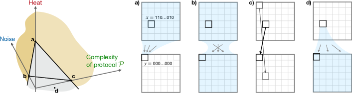
Figure 2: Illustration of our results using the erasure task, where an input string $x$ is mapped to an output $y$ consisting of all 0s, possibly in a noisy fashion. Four different processes that achieve our bound (13): a) Landauer erasure, where all possible inputs are mapped to the target $y$. b) Free expansion, where all inputs are allowed to thermalize to a uniform equilibrium distribution. c) Swap, where a single input and a single output are swapped, while all other states are left in place. d) Controlled expansion, where a single input is allowed to thermalize to a uniform equilibrium distribution.

IV Examples

To make things concrete, we now illustrate our results using two examples. In both examples, we consider a hard drive with $2^{n}$ logical states, encoding all bit strings of length $n\gg 1$. We consider two tasks. The first is the “erasure” task mentioned in the Introduction, which involves transforming a long incompressible string into a string of all zeros. The second is a “randomization” task, which involves transforming a string of all zeros into a long incompressible output.

IV.1 Example 1: Erasure

We first consider the erasure task, where we map a long incompressible input $x$ of length $n$ to an output $y$ consisting of $n$ zeros. In this case, $K(x|y)\approx K(x)\approx n$. We sketch out four different types of processes, illustrated in 2, that perform the erasure. We demonstrate that each type of process saturates our thermodynamic bounds (10) and (13) in a different way. In doing so, we also demonstrate that these two bounds are equivalent for these processes.

1) Landauer erasure, 2a). The Hamiltonian of the computational subsystem $A$ is set to zero and the subsystem is allowed to relax to a uniform equilibrium. The Hamiltonian is then quasistatically changed so that the system moves to an equilibrium distribution which is (nearly) a delta-function centered at the all-0s string. In the limit of quasistatic driving and peaked final energy functions, $Q(x\shortrightarrow y)\approx{\textstyle\frac{\ln 2}{\beta}}n$ and $-\log_{2}p(y|x)\approx 0$. This protocol has a simple description, $K(\mathcal{P})\approx 0$, so (9) implies that our two bounds (10) and (13) have the same minimal cost, $K(x|y,\mathcal{P}^{*})\approx K(x|y)\approx n$. Both bounds are achieved, with the minimal cost paid by heat.

2) Free expansion, 2b). This is simply the first part of the Landauer erasure process described above: the Hamiltonian of the subsystem $A$ is set to zero and the subsystem is again allowed to relax to a uniform equilibrium. Since each final state is equally likely under this free relaxation, $-\log_{2}p(y|x)=n$. No heat is released or absorbed, $Q(x\shortrightarrow y)=0$. This protocol has a simple description, $K(\mathcal{P})\approx 0$, so our two bounds (10) and (13) again have the same minimal cost, $K(x|y,\mathcal{P}^{*})\approx K(x|y)\approx n$. Both bounds are achieved, with the minimal cost is paid for by noise.

3) Swap, 2c). Subsystem $A$ undergoes a unitary that swaps the incompressible input string $x$ with the simple (all 0s) output string $y$, while all other states are left untouched. This process is deterministic, $-\log_{2}p(y|x)=0$, and no heat is exchanged with the bath, $Q(x\shortrightarrow y)=0$. However, this process requires that the input state $x$ be “hard coded” into the the unitary that implements the swap, so $K(\mathcal{P})\approx n$ and $K(x|y,\mathcal{P}^{*})\approx 0$. The minimal cost in (10) vanishes, $K(x|y,\mathcal{P}^{*})\approx 0$; this bound is achieved since both heat and noise vanish. The minimal cost in (13) is $K(x|y)\approx n$; this bound is again achieved and the cost is paid for by protocol complexity.

4) Controlled expansion, 2d). The Hamiltonian of subsystem $A$ is initially set to a peaked function at the target input $x$, and the subsystem is allowed to relax an equilibrium distribution which is (nearly) a delta-function centered at $x$. The Hamiltonian is then quasistatically changed to a constant energy function, so that the system moves to a uniform equilibrium distribution. In the limit of quasistatic driving and peaked initial energy function, heat can be extracted from the bath, $Q(x\shortrightarrow y)\approx-{\textstyle\frac{\ln 2}{\beta}}n$. However, this process is noisy, $-\log_{2}p(y|x)\approx n$. In addition, the initial Hamiltonian must include a description of the target input state $x$. Therefore, as for the Swap, $K(\mathcal{P})\approx n$ and $K(x|y,\mathcal{P}^{*})\approx 0$. The minimal cost in (10) vanishes, $K(x|y,\mathcal{P}^{*})\approx 0$; this bound is achieved since the heat and noise terms cancel. The minimal cost in (13) is $K(x|y)\approx n$; this bound is also achieved and the cost is paid for by a combination of absorbed heat, noise, and protocol complexity.

IV.2 Example 2: Randomization

We now consider the randomization task, where an input $x$ consisting of $n$ zeros is mapped to an output $y$ that is long and incompressible, $K(y)\approx n$. Since the input is very simple, we have $K(x|y)\approx K(x|y,\mathcal{P}^{*})\approx 0$. From a logical perspective, this task may be considered to be the opposite of erasure, in that the output and input roles are swapped. However, as we will see, the thermodynamic properties of the two tasks are very different.

We again consider the four types of processes mentioned in the previous section. We show that for the randomization task, the two thermodynamics bounds (10) and (13) can be different. We also show that only some of the processes can saturate the tighter bound (10).

1) Landauer reset. Subsystem $A$ is allowed to freely relax to a uniform equilibrium. The Hamiltonian is then quasistatically changed so that the system moves to an equilibrium distribution which is (nearly) a delta-function centered at the string $y$. In the limit of quasistatic driving and peaked final energy functions, $Q(x\shortrightarrow y)\approx{\textstyle\frac{\ln 2}{\beta}}n$ and $-\log_{2}p(y|x)\approx 0$. Plugging into (10) gives $n>0$ (up to additive constants), so the bound is not tight. Since the protocol must contain a description of $y$, we also have $K(\mathcal{P})\approx n$. Plugging into the weaker bound (13) shows that it is even looser, $2n>0$.

2) Free expansion. Subsystem $A$ is allowed to relax to a uniform equilibrium. Since each final state is equally likely under this free relaxation, $-\log_{2}p(y|x)=n$, and no heat is released or absorbed, $Q(x\shortrightarrow y)=0$. Plugging into (10) gives $n>0$, so the bound is not tight. In this case, the protocol is very simple, $K(\mathcal{P})\approx 0$, so (13) also gives $n>0$.

3) Swap. Subsystem $A$ undergoes a unitary that swaps $x$ and $y$, while all other states are left untouched. This process is deterministic, $-\log_{2}p(y|x)=0$, and no heat is exchanged with the bath, $Q(x\shortrightarrow y)=0$. In this case, the bound (10) is achieved. However, the protocol must contain a description of $y$, so $K(\mathcal{P})\approx n$. Therefore, the weaker bound (13) is not tight, $n>0$.

4) Controlled expansion. The Hamiltonian of subsystem $A$ is initially set to a peaked function at the target input $x$, and the system is allowed to relax to an equilibrium distribution which is (nearly) a delta-function centered at $x$. The Hamiltonian is then quasistatically changed to a constant energy function, so that the system moves to a uniform equilibrium distribution. In the limit of quasistatic driving and peaked initial energy function, heat can be extracted from the bath, $Q(x\shortrightarrow y)\approx-{\textstyle\frac{\ln 2}{\beta}}n$. However, this process is noisy, $-\log_{2}p(y|x)\approx n$. The bound (10) is achieved, since the noise and heat terms cancel. However, the protocol must contain a description of $y$, so $K(\mathcal{P})\approx n$. Therefore, the weaker bound (13) is not tight, $n>0$.

As we see, although the erasure and randomization tasks are similar from a logical standpoint, thermodynamically they are quite different. In general, our bound (10) can only be achieved when the system is not allowed to thermalize to a uniform distribution at the beginning of the process. This is because any such thermalization dissipates initial order, i.e., it tends to map the simple input $x$ to a $n$-bit string sampled from the uniform distribution, which almost always has high complexity (livi08, ). This is why erasure and randomization tasks differ: in the erasure task, an initial thermalization tends to replace the complex input $x$ with another complex string. It may be said that the complex input in the erasure task is “in equilibrium” with respect to the uniform distribution, while the simple input in the randomization task is “out of equilibrium” with respect to the uniform distribution.

V Relation to prior work

We briefly compare our results with prior work.

We first consider Zurek’s bound (3), as proposed in Ref. (zure89a, ). That result is a special case of (13), which applies to deterministic computations ($-\log p(x|y)=0$). Our bound is more general because it also applies to noisy processes, and because it explicitly highlights the dependence on protocol complexity. Perhaps more importantly, our bound is derived from a Hamiltonian formulation, which extends it to both quantum and classical systems while avoiding certain problematic aspects of the original derivation (see also discussion in (wolpert2019stochastic, ; kolchinsky2020thermodynamic, )).

Let us review the derivation of the original result, which used a two-step process (zure89a, ). First, the input $x$ is mapped to the pair of strings $(y,s)$, where $s$ is an auxiliary binary string that allows $x$ to be recovered from $(y,s)$ using some computer program. By construction, this first step is logically reversible, so in principle it can be carried out without generating heat. Second, the string $s$, which is stored in $\ell(s)$ binary degrees of freedom, is reset to all 0s. The cost of this erasure was argued to be $Q\geq{\textstyle\frac{\ln 2}{\beta}}\ell(s)$, as follows from Landauer’s bound (1). Finally, (3) follows since $x$ is decodable from $s$ and $y$, therefore $\ell(s)\geq K(x|y)+O(1)$ according to the definition of conditional Kolmogorov complexity (2) (here $O(1)$ is a constant that reflects the choice of the universal computer).

There are two problematic aspects of using Landauer’s principle to say that ${\textstyle\frac{\ln 2}{\beta}}\ell(s)$ is the minimal heat needed to reset $\ell(s)$ binary degrees of freedom (the same statement also appears in other related work (zure89a, ; bennett1993thermodynamics, ; bennett1998information, ; baumeler2019free, )). The first problem is that Landauer’s bound constrains the average heat across a statistical ensemble of inputs. For any individual input $x$ and individual auxiliary string $s$, the reset protocol can be designed to achieve much lower heat generation. In the extreme case, $s$ may be “hard coded” into the reset protocol, so that the reset generates no heat at all (as in the example shown in 2c). For this reason, a proper accounting of the second step should also include the complexity of the reset protocol, analogous to the term $K(\mathcal{P})$ that appears in our result . The second problem with the use of Landauer’s bound is more technical. Suppose that the reset protocol does not have any hard-coded information about the string $s$. Then, in order to reset $\ell(s)$ binary degrees of freedom at the Landauer cost of ${\textstyle\frac{\ln 2}{\beta}}\ell(s)$, the protocol must have information about the string length $\ell(s)$, which will vary between different inputs (wolpert2019stochastic, ). If this length is measured before running the reset, then this information about $\ell(s)$ also has to be erased, resulting in additional $O(\log\ell(s))$ heat generation. In fact, such logarithmic correction terms are unavoidable when trying to erase an arbitrary binary string of arbitrary length. (This problem can be avoided by appropriate use of self-delimiting codes during the erasure process, as done in our construction in Appendix B).

In our own recent work, we rederived a version of Zurek’s bound (3) using modern methods (kolchinsky2020thermodynamic, ). Although our derivation did not make use of Landauer’s bound as an intermediate step, it only applied to classical and deterministic computations. In addition, unlike the result presented here, it relied on idealized assumptions (such as the assumption of an idealized bath).

Finally, our approach should be contrasted with “single-shot thermodynamics” as recently considered in quantum thermodynamics and quantum information theory (aaberg2013truly, ; faist2015minimal, ; rio2011thermodynamic, ; tomamichelQuantumInformationProcessing2016, ; horodecki2013fundamental, ). Single-shot thermodynamics focuses on the thermodynamic costs and benefits incurred by individual computations at a guaranteed high probability, relative to some input ensemble. For this reason, single-shot costs are still defined in terms of statistical ensembles (faist2015minimal, ). In general, the goals of single-shot thermodynamics are different from our goals, which is to derive an algorithmic bound on the cost of a (deterministic or noisy) computation that does not reference any input ensemble.

VI Discussion

In this paper, we identified a fundamental thermodynamic bound on the cost of an individual computation. Our bound, which makes no reference to the statistical ensemble of inputs, was derived by combining ideas from two different lines of research. The first is algorithmic information theory (AIT), which defines information at the level of individual strings, rather than statistical ensembles. The second is stochastic thermodynamics, which defines thermodynamic quantities at the level of individual trajectories, rather than ensembles of trajectories.

The main assumption used to derive our results, and the most unusual one in the physics literature, is the computability assumption, which says that there exists a program that approximates the values of $p(y,c|x,b)$, $\beta$, and $\epsilon_{b}$ to arbitrary precision. It may be difficult to imagine a physical unitary or observable which cannot be calculated numerically using a finite program. Nonetheless, such non-computable unitaries and observables do exist in a mathematical sense (nielsen1997computable, ), although it is not clear whether they can be realized in any real-world physical system. The so-called “Physical Church-Turing thesis” (PCT), whose validity is the subject of ongoing discussion, postulates that non-computable unitaries and observables are not physically realizable (gandy1980church, ; deutsch1985quantum, ; geroch1986computability, ; braverman2015space, ). If the PCT is true, then our computability assumption is satisfied by all protocols that can be realized in real-world physical systems. If the PCT is not true, then there exists some physically realizable protocol $\mathcal{P}$ that does not satisfy the computability assumption — that is, it does not have a minimal description $\mathcal{P}^{*}$, so (10) does not apply. In general, our results point to an interesting relationship between PCT and thermodynamics.

There are several possible directions for future research. As mentioned in Section III.1, our results may be understood as “algorithmic fluctuation theorems”, that is algorithmic versions of detailed fluctuation theorems from stochastic thermodynamics. One may investigate there other results from stochastic thermodynamics, such as thermodynamic uncertainty relations (horowitz2020thermodynamic, ) and thermodynamic speed limits (shiraishi_speed_2018, ), may also have algorithmic analogues.

Another interesting research direction would extend our approach to fully quantum computations. As discussed in Section II.3, even though our analysis applies to quantum processes, the computation is operationalized using a two-point measurement scheme, in which a fixed reference basis is used to initialize the input and determine the output via a projective measurement. Therefore, the overall computation that maps the input string $x$ to the output string $y$ is classical, even if the process may use quantum effects at intermediate stages. In future work, it may be interesting to investigate the thermodynamic cost of a quantum computation that maps some input pure state $|\psi\rangle\langle\psi|$ to some output pure state $|\phi\rangle\langle\phi|$, without assuming that $|\psi\rangle\langle\psi|$ and $|\phi\rangle\langle\phi|$ belong to any fixed basis or result from projective measurements.

APPENDIX A DERIVATION OF (10)

Here we derive our main result, (10). We begin by proving the following useful inequality,

$$-\log_{2}p(y|x)+{\textstyle\frac{\beta}{\ln 2}}Q(x\shortrightarrow y)\geq-\log_{2}\tilde{p}(x|y),$$ (15)

where $p(y|x)$ is defined as in (5) and

$$\tilde{p}(x|y):=\sum_{b,c}p(y,c|x,b)\pi(c).$$ (16)

Note that $p(y,c|x,b)=|\langle y,c|U|x,b\rangle|^{2}=|\langle x,b|U^{\dagger}|y,c\rangle|^{2}$, which can be interpreted as the conditional probability of observing final state $|x,b\rangle$ given initial state $|y,c\rangle$ under the adjoint unitary evolution $U^{\dagger}$. Therefore $\sum_{x,b}p(y,c|x,b)=1$ and $\sum_{x}\tilde{p}(x|y)=1$, meaning that $\tilde{p}(x|y)$ is a normalized conditional probability distribution. In addition, the adjoint unitary $U^{\dagger}$ can be understood as the time-reversal of the actual unitary $U$ (campisi2011colloquium, ; manzanoQuantumFluctuationTheorems2018, ). Therefore, $\tilde{p}(x|y)$ can also be seen as the probability of output $x$ from input $y$ under the time-reversed process.

Next, write the following identity

$$p(y,c|x,b)\pi(c)=p(y,c|x,b)\pi(b)e^{-\beta(\epsilon_{c}-\epsilon_{b})}.$$ (17)

We sum both sides of (17) over the initial and final bath states $b$ and $c$ to give

$$\tilde{p}(x|y) =\sum_{b,c}p(y,c|x,b)\pi(b)e^{-\beta(\epsilon_{c}-\epsilon_{b})}$$

$$=p(y|x)\sum_{b,c}\frac{p(y,c|x,b)\pi(b)}{p(y|x)}e^{-\beta(\epsilon_{c}-\epsilon_{b})}$$

$$\geq p(y|x)e^{-\beta Q(x\shortrightarrow y)}.$$ (18)

In the first line, we used the definition of $\tilde{p}(x|y)$ from (16). In the second line, we used the definition of $p(y|x)$ from (5). In the last line, we used Jensen’s inequality and the definition of $Q(x\shortrightarrow y)$ from (6). Rearranging (18) gives (15). The inequality (18) becomes tight when heat fluctuations become small, which is expected in the limit of a large self-averaging heat bath and slow driving. This inequality appears as (12) in the main text. We note that this type of derivation is often used to prove detailed fluctuation theorems in stochastic thermodynamics (jarzynski2000hamiltonian, ; sagawa2012fluctuation, ; kwonFluctuationTheoremsQuantum2019, ; BuscemiBayesianRetrodiction2021, ; jarzynski2004classical, ; manzanoQuantumFluctuationTheorems2018, ).

Next, we introduce the bound

$$-\log_{2}\tilde{p}(x|y)+\gamma_{\mathfrak{C}}\geq K(x|y,\mathcal{P}^{*}),$$ (19)

where $K(x|y,\mathcal{P}^{*})$ is the conditional Kolmogorov complexity described in Section II.2, and $\gamma_{\mathfrak{C}}$ is a constant that does not depend on $x$, $y$, or $\mathcal{P}$. While (19) is a standard result in AIT (vitanyi2013conditional, ), here we sketch out its proof at a high level. Recall that $\mathcal{P}^{*}$ is a program that computes the values of $p(y,c|x,b)$ and $\pi(b)$ to arbitrary precision (7). Next, we define the following program which outputs $x$ when provided with $y$ and $\mathcal{P}^{*}$ as input:

1. It calculates the conditional probability distribution $x^{\prime}\mapsto\tilde{p}(x^{\prime}|y)$ for the given $y$ and all $x^{\prime}\in\{0,1\}^{*}$. This is done by running the provided program $\mathcal{P}^{*}$ and computing $\tilde{p}(x^{\prime}|y)$ via (16).

2. Using the conditional probability distribution $\tilde{p}(x^{\prime}|y)$, it constructs a codebook, a function that maps codewords $s\in\{0,1\}^{*}$ to strings $x^{\prime}\in\{0,1\}^{*}$. Using a standard coding algorithm, such as Shannon-Fano coding or Huffman coding, the codeword $s_{x^{\prime}}$ assigned to string $x^{\prime}$ may be chosen to have length $\ell(s_{x^{\prime}})\leq\left\lceil-\log_{2}\tilde{p}(x^{\prime}|y)\right\rceil$.

3. The program contains a copy of the codeword $s_{x}$ that maps to string $x$. It looks up this codeword in the generated codebook and prints the resulting string $x$.

The length of this program is no more than

$$\ell(s_{x})+\gamma_{\mathfrak{C}}\leq-\log_{2}\tilde{p}(x^{\prime}|y)+\gamma_{\mathfrak{C}}+1,$$

where $\gamma_{\mathfrak{C}}$ is an additive constant that reflect the length of the algorithm needed to compute the conditional distribution $\tilde{p}(x^{\prime}|y)$ (while calling $\mathcal{P}^{*}$ as a subroutine), generate the codebook, and look up the codeword $s_{x}$. The bound (19) follows after absorbing 1 into the additive constant $\gamma_{\mathfrak{C}}$, since $K(x|y,\mathcal{P}^{*})$ is the length of the shortest program that outputs $x$ when provided with $y$ and $\mathcal{P}^{*}$ as input.

Combining with (19) and (15) gives (10).

APPENDIX B ACHIEVABILITY OF (10)

Step	Description	State of $X\times M$ at end of step	Heat for input $x$ and output $y$
Initialize	Subsystems $X\times M$ begin with the initial Hamiltonian $$H_{XM}=\sum_{x^{\prime},m}(\chi_{x^{\prime}}+\mu_{m})|x^{\prime},m\rangle\langle x^{\prime},m|.$$ (20)	$|x,\varnothing\rangle\langle x,\varnothing|$
Copy	Input state $|x\rangle$ is copied from $X$ into $M$ using unitary over $X\times M$.	$|x,x\rangle\langle x,x|$
Quench 1	Hamiltonian $H_{XM}$ is quenched from (20) to $$H_{XM}=\sum_{x^{\prime},m}(\chi_{x^{\prime}}+\mu_{m}-\eta\delta_{x^{\prime},m})|x^{\prime},m\rangle\langle x^{\prime},m|.$$ (21)	$|x,x\rangle\langle x,x|$
Relax 1	$X$ freely relaxes to conditional equilibrium for $H_{XM}$, while $M$ is held fixed.	$\approx|x,x\rangle\langle x,x|$	$\approx 0$
Compute	Hamiltonian $H_{XM}$ is quasistatically changed to $$H_{XM}=\sum_{y^{\prime},m}[-\beta^{-1}\ln p(y^{\prime}|m)+\mu_{m}]|y^{\prime},m\rangle\langle y^{\prime},m|,$$ (22) during which $X$ is allowed to relax to equilibrium and $M$ is held fixed.	$\approx{\displaystyle\sum_{y^{\prime}}p(y^{\prime}|x)|y^{\prime},x\rangle\langle y^{\prime},x|}$	$\approx\beta^{-1}\ln p(y|x)$
Quench 2	Hamiltonian $H_{XM}$ is quenched from (22) to $$H_{XM}=\sum_{y^{\prime},m}\omega_{y^{\prime}m}|y^{\prime},m\rangle\langle y^{\prime},m|.$$ (23)
Relax 2	$M$ freely relaxes to conditional equilibrium for (23) while $X$ is held fixed.	$\approx{\displaystyle\sum_{y^{\prime},m}p(y^{\prime}|x)q_{\omega}^{\text{eq}}(m|y^{\prime})}$ $\times|y^{\prime},m\rangle\langle y^{\prime},m|$	$\approx\omega_{yx}-\langle\omega\rangle_{q_{\omega}^{\text{eq}}(M|y)}$
Reset	Hamiltonian $H_{XM}$ is quasistatically changed to $$H_{XM}=\sum_{y^{\prime},m}(\chi_{y^{\prime}}+\mu_{m}-\eta\delta_{\varnothing,m})|y^{\prime},m\rangle\langle y^{\prime},m|,$$ (24) during which $M$ is allowed to relax to equilibrium and $X$ is held fixed.	$\approx{\displaystyle\sum_{y^{\prime}}p(y^{\prime}|x)|y^{\prime},\varnothing\rangle\langle y^{\prime},\varnothing|}$	$\approx\text{$\beta^{-1}$}S(q_{\omega}^{\text{eq}}(M|y))$
Final quench	Hamiltonian $H_{XM}$ is quenched to the initial Hamiltonian in (20).	$\approx{\displaystyle\sum_{y^{\prime}}p(y^{\prime}|x)|y^{\prime},\varnothing\rangle\langle y^{\prime},\varnothing|}$

Table 1: Description of the 9-step protocol that implements a stochastic input-output map that is arbitrarily close to some desired $p(y|x)$, while achieving a heat dissipation arbitrarily close to the bound (10). $\delta$ is the Kronecker delta function.

Here we show that the bound (10) can be achieved.

B.1 Protocol Construction

Formally, we imagine that we are provided with some desired input-output conditional probability distribution $p_{Y|X}$. We also imagine that we are provided with a thermal environment with inverse temperature $\beta$ and energy function $\epsilon$. We assume that these are all computable, meaning that there exists some computer program that can output the value of any $p(y|x)$, any $\epsilon_{b}$, and $\beta$ to any desired degree of precision. We also assume that the heat bath described by $\epsilon$ and $\beta$ is nearly ideal, i.e., it is large and undergoes rapid self-equilibration. Then, in the limit of an ideal bath, we show that there exists a protocol $\mathcal{P}$ that can come arbitrarily closely to the bound (10). We do so by sketching out the construction of such a protocol $\mathcal{P}$ at a high level, without delving into full technical rigor which would go beyond the scope of this paper.

Our construction will suppose that subsystem $X$ has access to an additional “memory subsystem” $M$. The memory subsystem has the same dimensionality as $X$ and it acts as a catalyst: it is initialized in an unentangled “empty string” pure state $|\varnothing\rangle$ at the beginning of the protocol, and it is left in (nearly) the same pure state after the protocol finishes. We will perform protocols on $X$ that depend on the state of $M$ while holding the state of $M$ fixed — and vice versa for protocols over $M$ with $X$ held fixed. Such protocols are often termed “feedback control” in the literature (sagawa2008second, ; parrondo2015thermodynamics, ).

We will also use the fact that a nearly ideal bath can be weakly coupled to subsystems $X\times M,$ and then used to carry out transformations over $X\times M$ in a (nearly) quasistatic and thermodynamically reversible manner (see constructions in (anders2013thermodynamics, ; reeb_improved_2014, ; aaberg2013truly, ; skrzypczyk2014work, )). Weak coupling also allows us to write the First Law as $Q=W-\Delta E_{XM}$, where $Q$ is generated heat, $W$ is work done on the system, and $\Delta E_{XM}$ is the expected energy increase of subsystems $X\times M$.

Our protocol consists of 9 steps, which are described in 1. The third column in 1 shows the approximate state of subsystems $X\times M$ at the end of each step. (The approximations become exact in the limit of slow driving, idealized bath, complete relaxation to equilibrium, and infinitely peaked energy functions $\eta\to\infty$.) It can be verified that the protocol maps $X$ from input state $|x\rangle$ to output state $|y\rangle$ sampled from $\approx p(y|x)$, while the memory subsystem $M$ starts and ends arbitrarily close to the pure state $|\varnothing\rangle$. Note also that the protocol starts and ends on the same Hamiltonian, (20). The protocol is effectively classical, in that it does not exploit coherence or entanglement, even though it may be implemented on a quantum system.

We emphasize a few aspects of our construction. First, the Copy step does not violate the no-cloning theorem, since $|x\rangle$ is assumed to come from the fixed orthonormal basis $\{|a\rangle\}_{a\in\{0,1\}^{*}}$. Second, two of the steps (Compute and Reset) involve thermodynamically reversible feedback control operations, as discussed above (see also (Section 5.1, reeb_improved_2014, )). Third, there are three energy functions $\chi,\mu,\omega$ and a scalar $\eta$ that appear in our construction, which may be chosen somewhat arbitrarily. The energy functions $\chi$ and $\mu$, which appear in (20), (21), (22), and (24), refer to arbitrary “baseline” energy values for $X$ and $M$ respectively. The scalar $\eta\gg 0$ refers to a large energy value that favors equilibrium correlations between $X$ and $M$ under the Hamiltonian (21), and favors equilibrium reset of $M$ to state $|\varnothing\rangle$ under the Hamiltonian (24). We usually consider very large $\eta$, approaching the limit $\eta\to\infty$. The energy function $\omega$ in (23) refers to a set of energy values over $X\times M$, which we will return to below. Below we will assume that $\chi,\mu,\omega$ and $\eta$ are algorithmically simple (i.e., there exists a short program to compute their values).

We now calculate the heat generated by this protocol during the computation $x\shortrightarrow y$. The approximate amount of heat generated by each step of the protocol, conditioned on input $|x\rangle$ and output $|y\rangle$, is shown in the last column of 1 (as above, the approximations become exact under appropriate limits). We describe the calculated heat values in more depth. Copy involves a unitary over $X\times M$, so it does not involve any heat exchange. The three quench steps (Quench 1, Quench 2, Final Quench) refer to (nearly) instantaneous changes of the Hamiltonian, so they also do not involve any heat exchange.

Relax 1 does not involve driving, therefore the heat is given by the decrease of the energy of subsystem $X\times M$ due to the change of the statistical state. In fact, the statistical state does not change (in the limit $\eta\to\infty$) and so heat vanishes. For Relax 2, the heat is also equal to the decrease of the energy of $X\times M$ due to the change of the statistical state. Conditioned on input $x$ and output $y$, subsystems $X\times M$ are (nearly) in pure state $|y,x\rangle\langle y,x|$ at the beginning of this step. At the end of this step, subsystem $M$ is found in the conditional equilibrium distribution

$$q_{\omega}^{\text{eq}}(M=m|X=y)=e^{-\beta(\omega_{ym}-F_{M|X=y}^{\omega})},$$ (25)

where we defined the conditional free energy

$$F_{M|X=y}^{\omega}=-\frac{1}{\beta}\ln\sum_{m}e^{-\beta\omega_{ym}}.$$ (26)

To calculate the heat generated by Compute, we use the First Law of Thermodynamics, $Q=W-\Delta E_{XM}$. We also use that in the quasistatic and classical limit, work is equal to the increase of the equilibrium free energy of $X\times M$ and work fluctuations vanish (speck2004distribution, ; scandi2020quantum, ). Since $M$ is held fixed in state $|x\rangle$, we consider the increase of the conditional free energy, $W\approx\Delta F_{X|M=x}$. Then, observe that in this step, $X\times M$ is transformed from the pure state $|x,x\rangle\langle x,x|$ with Hamiltonian (21) to the mixed state $\sum_{y^{\prime}}p(y^{\prime}|x)|y^{\prime},x\rangle\langle y^{\prime},x|$ with Hamiltonian (22), so

$$\Delta F_{X|M=x} =-\frac{1}{\beta}\ln\sum_{y}e^{\ln p(y|x)-\beta\mu_{x}}-(\chi_{x}+\mu_{x}-\eta)$$

$$=\mu_{x}-(\chi_{x}+\mu_{x}-\eta).$$

The change of energy of $X\times M$, conditioned on input $x$ and output $y$, is $\Delta E_{XM}\approx-\beta^{-1}\ln p(y|x)+\mu_{x}-(\chi_{x}+\mu_{x}-\eta)$. Plugging into $Q\approx\Delta F_{X|M=x}-\Delta E_{XM}$ gives $Q\approx\beta^{-1}\ln p(y|x)$, as found in 1.

For Reset, we use that the heat generated by a thermodynamically reversible feedback control operation, where $M$ is modified while $X$ is held fixed, is $\beta^{-1}$ times the decrease of the conditional Shannon entropy $S(M|X)$ (reeb_improved_2014, ). Since subsystem $X$ is observed in output state $y$ at the end of the process, and since it does not change in between Reset and the end of the process, it must be in state $y$ during this step. Thus, we consider the decrease of the conditional Shannon entropy $S(M|X=y)$. The conditional distribution over energy eigenstates of $M$ at the beginning of this step is (approximately) $q_{\omega}^{\text{eq}}(M=m|X=y)$. At the end of this step, $M$ is (nearly) in the pure state $|\varnothing\rangle$, independently of the state of $X$, so the conditional Shannon entropy vanishes. Combining gives the result in 1.

Summing together the heat values in 1 implies that the overall generated heat is

$$Q(x\shortrightarrow y)\approx\frac{1}{\beta}\ln p(y|x)+\omega_{yx}-F_{M|X=y}^{\omega},$$ (27)

where we used the identity $F_{M|X=y}^{\omega}=\langle\omega\rangle_{q_{\omega}^{\text{eq}}(M|y)}-\beta^{-1}S(q_{\omega}^{\text{eq}}(M|y))$.

B.2 Sketch of proof of achievability

We now show that the protocol $\mathcal{P}$ described above can approach the bound (10). We imagine there is some desired computation $p_{Y|X}$, as well as a nearly ideal heat bath described by the inverse temperature $\beta$ and energy function $\epsilon$. We use $\mathcal{R}=(p_{Y|X},\epsilon,\beta)$ to refer to the details of the computation. Importantly, we assume that $\mathcal{R}$ is computable. We show that the corresponding nine-step protocol $\mathcal{P}$, as defined in the previous subsection, comes close to equality in (10).

It must be emphasized that in the following, the protocol $\mathcal{P}$ is treated as a function of the desired computation $\mathcal{R}$. For this reason, the additive constant $O(1)$ that appears below refers to a quantity that doesn’t depend on $x$, $y$, or the desired computation $\mathcal{R}$. Similarly, within the family of protocols defined in the last subsection, $\gamma_{\mathfrak{C}}$ in (10) should be understood as an additive constant that doesn’t depend on $x$, $y$, or the details of the computation $\mathcal{R}$.

To begin, we define some algorithmic information measures. Let $\mathcal{R}^{*}\in\{0,1\}^{*}$ refer to the shortest program for the universal computer $\mathfrak{C}$ that computes the conditional distribution $p_{Y|X}$, energy function $\epsilon$, and inverse temperature $\beta$ to arbitrary precision. In addition, let $K(x|y,\mathcal{R}^{*})$ indicate the length of the shortest program that produces $x$ when provided with $y$ and $\mathcal{R}^{*}$ as side information and let $K(\mathcal{R}|y,\mathcal{P}^{*})$ indicate the length of the shortest program for computing $(p_{Y|X},\epsilon,\beta)$ given $y$ and $\mathcal{P}^{*}$ as side information (recall that $\mathcal{P}^{*}$ is the shortest program for computing the values (7) for our protocol). Finally, let $K(\mathcal{P}|y,\mathcal{R}^{*})$ indicate the length of the shortest program for computing values (7) given $y$ and $\mathcal{R}^{*}$ as side information.

In addition, let $\mathfrak{D}$ indicate some computable compression algorithm with side information (e.g., Lempel-Ziv compression with side information). Let $\ell_{\mathfrak{D}}$ indicate the length of a program implementing this compression algorithm. Importantly, we assume that this algorithm is simple in the sense that $\ell_{\mathfrak{D}}=O(1)$. In addition, let $c(x|y,\mathcal{R}^{*})$ indicate the length of the self-delimiting codeword produced by this algorithm for $x$ when provided with side information $y$ and $\mathcal{R}^{*}$. Without loss of generality, we assume that the codebook that defines $c(x|y,\mathcal{R}^{*})$ is complete for all $y$, so that Kraft’s inequality holds with equality (cover_elements_2006, ; livi08, ), $\sum_{x}2^{-c(x|y,\mathcal{R}^{*})}=1$.

Recall that we are free to choose any set of energy values $\omega$ in (23), as long as the conditional free energy $F_{M|X=y}^{\omega}$ is finite and $q_{\omega}^{\text{eq}}(x|y)$ is a normalized conditional distribution. We define these energy values $\omega$ as

$${\textstyle\frac{\beta}{\ln 2}}\omega_{yx}=\ell_{\mathfrak{D}}+c(x|y,\mathcal{R}^{*}),$$ (28)

Using $\sum_{x}2^{-c(x|y,\mathcal{R}^{*})}=1$ and (26), we calculate that $F_{M|X=y}^{\omega}=\frac{\ln 2}{\beta}\ell_{\mathfrak{D}}$. Plugging into (27) and rearranging gives

$${\textstyle\frac{\beta}{\ln 2}}Q(x\shortrightarrow y)\approx\log_{2}p(y|x)+c(x|y,\mathcal{R}^{*}).$$ (29)

Note that better compression algorithms, which have smaller code lengths, lead to lower heat production.

A known result from AIT states that conditional Kolmogorov complexities obey a type of “triangle inequality” (Lemma 3.9.1, livi08, ),

$$K(x|y,\mathcal{P}^{*}) \leq K(\mathcal{R}|y,\mathcal{P}^{*})+K(x|y,\mathcal{R}^{*})+O(1)$$

$$K(x|y,\mathcal{R}^{*}) \leq K(\mathcal{P}|y,\mathcal{R}^{*})+K(x|y,\mathcal{P}^{*})+O(1).$$

We will use this to show that

$$K(x|y,\mathcal{R}^{*})=K(x|y,\mathcal{P}^{*})+O(1).$$ (30)

Suppose that one is given $\mathcal{R}^{*}$ (which computes values of $p_{Y|X}$, $\epsilon$, and $\beta$) along with a program that computes the values of $\chi,\mu,\eta$ and $\omega$ that appear in the 9-step protocol outlined in Table 1. In that case, one could compute not only $\epsilon$ and $\beta$, but also the unitary $U$ that implements that protocol $\mathcal{P}$, giving the values of $p(y,c|x,b)=|\langle y,c|U|x,b\rangle|^{2}$ in (7). Thus, we may write

$$K(\mathcal{P}|y,\mathcal{R}^{*})\leq K(\chi,\mu,\eta|y,\mathcal{R}^{*})+K(\omega|y,\mathcal{R}^{*})+O(1).$$

Since $\chi$, $\mu$ and $\eta$ are arbitrary, we may assume that they can be produced by a simple program when provided with $y$ and $\mathcal{R}^{*}$ as side information, so $K(\chi,\mu,\eta|y,\mathcal{R}^{*})=O(1)$. (Note that the scaling $\eta\to\infty$ can be achieved without additional algorithmic cost by scaling $\eta$ as a function of the heat bath energy function $\epsilon$, as specified by $\mathcal{R}^{*}$). The values of $\omega$ are determined by $\beta$ plus the choice of the compression algorithm $\mathfrak{D}$, which obeys $\ell(\mathfrak{D})=O(1)$, hence $K(\omega|y,\mathcal{R}^{*})=O(1)$. Combining implies that $K(x|y,\mathcal{R}^{*})\leq K(x|y,\mathcal{P}^{*})+O(1)$. But it is also the case that $K(\mathcal{R}|y,\mathcal{P}^{*})=O(1)$, since if one had a program to compute the values (7) that define $\mathcal{P}$, one could easily compute $\epsilon$, $\beta$, and $p_{Y|X}$ (the latter via (5)). Therefore $K(x|y,\mathcal{P}^{*})\leq K(x|y,\mathcal{R}^{*})+O(1)$. Combining implies (30).

Finally, we have that

$$c(x|y,\mathcal{R}^{*}) =\ell_{\mathfrak{D}}+c(x|y,\mathcal{R}^{*})+O(1)$$

$$\geq K(x|y,\mathcal{R}^{*})+O(1)$$ (31)

$$=K(x|y,\mathcal{P}^{*})+O(1),$$ (32)

where in the first line we used $\ell_{\mathfrak{D}}=O(1)$, in the second line the definition of $K(x|y,\mathcal{R}^{*})$, and in the last line (30). Combining (29) and (32) then implies the bound

$$\frac{\beta}{\ln 2}Q(x\shortrightarrow y) \geq\log_{2}p(y|x)+K(x|y,\mathcal{P}^{*})+O(1).$$ (33)

The inequality in (33) can be made arbitrarily tight under an appropriate limit, which implies the achievability of our bound (10). Specifically, the inequality (29) can be made arbitrarily tight in the limit of slow driving, idealized bath, complete relaxation to equilibrium, and infinitely peaked energy functions $\eta\to\infty$. The inequality (31) can be made arbitrarily tight in the limit of increasingly good compression algorithms, so that $c(x|y,\mathcal{R}^{*})$ approaches the ultimate algorithmic bound $K(x|y,\mathcal{R}^{*})$ in (31). In fact, there are known techniques to construct a sequence of compression algorithms such that $c(x|y,\mathcal{R}^{*})$ approaches $K(x|y,\mathcal{R}^{*})$ for any finite set of $x$ and $y$. Such techniques are sometimes called “dovetailing” algorithms in the literature (livi08, ). (We note that the compression algorithm $\mathfrak{D}$ can “scale” the dovetailing parameter in line with the scaling of the heat bath, as specified by the side information $\mathcal{R}^{*}$, without incurring an additional algorithmic cost.)

At the same time, Kolmogorov complexity is uncomputable, so the convergence $c(x|y,\mathcal{R}^{*})\to K(x|y,\mathcal{R}^{*})$ cannot be uniform across $x$ and $y$, and in general one cannot know how far away from the ultimate limit is any given compression algorithm (livi08, ). To summarize, our bound (10) is achievable in the sense that it is possible to construct a sequence of thermal environments and physical protocols that come arbitrarily close to equality for any finite set of $x$ and $y$. At the same time, it is impossible to know how far in the sequence one must go in order to guarantee that, for any desired $x$ and $y$, the deficit in (10) is bounded by a constant.

References

- (1) R. Landauer, “Irreversibility and heat generation in the computing process,” IBM journal of research and development, vol. 5, no. 3, pp. 183–191, 1961.
- (2) C. H. Bennett, “The thermodynamics of computation—a review,” International Journal of Theoretical Physics, vol. 21, no. 12, pp. 905–940, 1982.
- (3) O. Maroney, “Generalizing Landauer’s principle,” Physical Review E, vol. 79, no. 3, p. 031105, 2009.
- (4) P. Faist, F. Dupuis, J. Oppenheim, and R. Renner, “The minimal work cost of information processing,” Nature communications, vol. 6, 2015.
- (5) J. M. Parrondo, J. M. Horowitz, and T. Sagawa, “Thermodynamics of information,” Nature Physics, vol. 11, no. 2, pp. 131–139, 2015.
- (6) A. Kolchinsky and D. H. Wolpert, “Dependence of dissipation on the initial distribution over states,” Journal of Statistical Mechanics: Theory and Experiment, p. 083202, 2017.
- (7) A. B. Boyd, D. Mandal, and J. P. Crutchfield, “Identifying functional thermodynamics in autonomous Maxwellian ratchets,” New Journal of Physics, vol. 18, no. 2, p. 023049, 2016.
- (8) T. E. Ouldridge and P. R. ten Wolde, “Fundamental costs in the production and destruction of persistent polymer copies,” Physical Review Letters, vol. 118, no. 15, p. 158103, 2017.
- (9) A. B. Boyd, “Thermodynamics of modularity: Structural costs beyond the Landauer bound,” Physical Review X, vol. 8, no. 3, 2018.
- (10) D. H. Wolpert, “The stochastic thermodynamics of computation,” arXiv:1905.05669v2, Please see corrected post-publication version, dated 2023-02-17.
- (11) D. H. Wolpert and A. Kolchinsky, “Thermodynamics of computing with circuits,” New Journal of Physics, 2020.
- (12) P. M. Riechers and M. Gu, “Initial-state dependence of thermodynamic dissipation for any quantum process,” Physical Review E, vol. 103, no. 4, p. 042145, 2021.
- (13) ——, “Impossibility of achieving landauer’s bound for almost every quantum state,” Physical Review A, vol. 104, no. 1, p. 012214, 2021.
- (14) A. Kolchinsky and D. H. Wolpert, “Dependence of integrated, instantaneous, and fluctuating entropy production on the initial state in quantum and classical processes,” Physical Review E, vol. 104, no. 5, p. 054107, 2021.
- (15) G. Kardeş and D. Wolpert, “Inclusive thermodynamics of computational machines,” arXiv preprint arXiv:2206.01165, 2022.
- (16) M. Li and P. Vitanyi, An Introduction to Kolmogorov Complexity and Its Applications. Springer, 2008.
- (17) P. M. Vitányi, “Conditional Kolmogorov complexity and universal probability,” Theoretical Computer Science, vol. 501, pp. 93–100, 2013.
- (18) W. H. Zurek, “Thermodynamic cost of computation, algorithmic complexity and the information metric,” Nature, vol. 341, pp. 119–124, 1989.
- (19) ——, “Algorithmic randomness and physical entropy,” Phys. Rev. A, vol. 40, pp. 4731–4751, Oct 1989.
- (20) C. H. Bennett, P. Gács, M. Li, P. Vitányi, and W. H. Zurek, “Thermodynamics of computation and information distance,” in Proceedings of the twenty-fifth annual ACM symposium on Theory of computing. ACM, 1993, pp. 21–30.
- (21) C. H. Bennett, P. Gács, M. Li, P. M. Vitányi, and W. H. Zurek, “Information distance,” Information Theory, IEEE Transactions on, vol. 44, no. 4, pp. 1407–1423, 1998.
- (22) Ä. Baumeler and S. Wolf, “Free energy of a general computation,” Physical Review E, vol. 100, no. 5, p. 052115, 2019.
- (23) A. Kolchinsky and D. H. Wolpert, “Thermodynamic costs of Turing machines,” Physical Review Research, vol. 2, no. 3, p. 033312, 2020.
- (24) K. Hiura and S.-i. Sasa, “Microscopic reversibility and macroscopic irreversibility: from the viewpoint of algorithmic randomness,” Journal of Statistical Physics, vol. 177, no. 5, pp. 727–751, 2019.
- (25) S. Ro, B. Guo, A. Shih, T. V. Phan, R. H. Austin, D. Levine, P. M. Chaikin, and S. Martiniani, “Model-free measurement of local entropy production and extractable work in active matter,” Physical Review Letters, vol. 129, no. 22, p. 220601, 2022.
- (26) L. d. Rio, J. Åberg, R. Renner, O. Dahlsten, and V. Vedral, “The thermodynamic meaning of negative entropy,” Nature, vol. 474, no. 7349, pp. 61–63, 2011.
- (27) P. Skrzypczyk, A. J. Short, and S. Popescu, “Work extraction and thermodynamics for individual quantum systems,” Nature communications, vol. 5, p. 4185, 2014.
- (28) K. V. Hovhannisyan, F. Barra, and A. Imparato, “Charging assisted by thermalization,” Physical Review Research, vol. 2, no. 3, p. 033413, 2020.
- (29) L. J. Schulman, T. Mor, and Y. Weinstein, “Physical limits of heat-bath algorithmic cooling,” Physical review letters, vol. 94, no. 12, p. 120501, 2005.
- (30) A. E. Allahverdyan, K. V. Hovhannisyan, D. Janzing, and G. Mahler, “Thermodynamic limits of dynamic cooling,” Physical Review E, vol. 84, no. 4, p. 041109, 2011.
- (31) S. Raeisi and M. Mosca, “Asymptotic bound for heat-bath algorithmic cooling,” Physical review letters, vol. 114, no. 10, p. 100404, 2015.
- (32) H. Tasaki, “Jarzynski relations for quantum systems and some applications,” arXiv preprint cond-mat/0009244, 2000.
- (33) M. Esposito, U. Harbola, and S. Mukamel, “Nonequilibrium fluctuations, fluctuation theorems, and counting statistics in quantum systems,” Reviews of modern physics, vol. 81, no. 4, p. 1665, 2009.
- (34) M. Campisi, P. Hänggi, and P. Talkner, “Colloquium: Quantum fluctuation relations: Foundations and applications,” Reviews of Modern Physics, vol. 83, no. 3, p. 771, 2011.
- (35) G. Manzano, J. M. Horowitz, and J. M. R. Parrondo, “Quantum Fluctuation Theorems for Arbitrary Environments: Adiabatic and Nonadiabatic Entropy Production,” Physical Review X, vol. 8, no. 3, Aug. 2018.
- (36) F. Buscemi and V. Scarani, “Fluctuation theorems from Bayesian retrodiction,” Phys. Rev. E, vol. 103, p. 052111, May 2021.
- (37) T. M. Cover and J. A. Thomas, Elements of information theory. John Wiley & Sons, 2006.
- (38) S. Deffner and C. Jarzynski, “Information processing and the second law of thermodynamics: An inclusive, Hamiltonian approach,” Physical Review X, vol. 3, no. 4, p. 041003, 2013.
- (39) D. P. DiVincenzo, “Quantum computation,” Science, vol. 270, no. 5234, pp. 255–261, 1995.
- (40) P. M. Vitányi, “Quantum kolmogorov complexity based on classical descriptions,” IEEE Transactions on Information Theory, vol. 47, no. 6, pp. 2464–2479, 2001.
- (41) A. Berthiaume, W. Van Dam, and S. Laplante, “Quantum kolmogorov complexity,” Journal of Computer and System Sciences, vol. 63, no. 2, pp. 201–221, 2001.
- (42) C. E. Mora, H. J. Briegel, and B. Kraus, “Quantum kolmogorov complexity and its applications,” International Journal of Quantum Information, vol. 5, no. 05, pp. 729–750, 2007.
- (43) C. H. Bennett, H. J. Bernstein, S. Popescu, and B. Schumacher, “Concentrating partial entanglement by local operations,” Physical Review A, vol. 53, no. 4, p. 2046, 1996.
- (44) T. Baumgratz, M. Cramer, and M. B. Plenio, “Quantifying coherence,” Physical Review Letters, vol. 113, no. 14, Sep. 2014.
- (45) C. Jarzynski, “Hamiltonian derivation of a detailed fluctuation theorem,” Journal of Statistical Physics, vol. 98, no. 1-2, pp. 77–102, 2000.
- (46) T. Sagawa and M. Ueda, “Fluctuation theorem with information exchange: Role of correlations in stochastic thermodynamics,” Physical Review Letters, vol. 109, no. 18, p. 180602, 2012.
- (47) H. Kwon and M. S. Kim, “Fluctuation Theorems for a Quantum Channel,” Physical Review X, vol. 9, no. 3, Aug. 2019.
- (48) H. Zenil, “A review of methods for estimating algorithmic complexity: options, challenges, and new directions,” Entropy, vol. 22, no. 6, p. 612, 2020.
- (49) J. Ziv, “Fixed-rate encoding of individual sequences with side information,” IEEE Transactions on Information Theory, vol. 30, no. 2, pp. 348–352, 1984.
- (50) P. Subrahmanya and T. Berger, “A sliding window lempel-ziv algorithm for differential layer encoding in progressive transmission,” in Proceedings of 1995 IEEE International Symposium on Information Theory. IEEE, 1995, p. 266.
- (51) T. Uyematsu and S. Kuzuoka, “Conditional lempel-ziv complexity and its application to source coding theorem with side information,” in IEEE International Symposium on Information Theory, 2003. Proceedings. IEEE, 2003, p. 142.
- (52) H. Cai, S. R. Kulkarni, and S. Verdú, “An algorithm for universal lossless compression with side information,” IEEE Transactions on Information Theory, vol. 52, no. 9, pp. 4008–4016, 2006.
- (53) R. Cilibrasi and P. M. Vitányi, “Clustering by compression,” IEEE Transactions on Information theory, vol. 51, no. 4, pp. 1523–1545, 2005.
- (54) M. B. Kennel, “Testing time symmetry in time series using data compression dictionaries,” Physical Review E, vol. 69, no. 5, p. 056208, 2004.
- (55) K. Dingle, C. Q. Camargo, and A. A. Louis, “Input–output maps are strongly biased towards simple outputs,” Nature communications, vol. 9, no. 1, pp. 1–7, 2018.
- (56) R. Avinery, M. Kornreich, and R. Beck, “Universal and accessible entropy estimation using a compression algorithm,” Physical review letters, vol. 123, no. 17, p. 178102, 2019.
- (57) It should be noted that the idea that the algorithmic complexity of the ensemble should also be included in a proper thermodynamic accounting appears in a different part of Zurek’s paper, (Eq. (23), zure89a, ).
- (58) J. Åberg, “Truly work-like work extraction via a single-shot analysis,” Nature communications, vol. 4, no. 1, pp. 1–5, 2013.
- (59) M. Tomamichel, Quantum Information Processing with Finite Resources, ser. SpringerBriefs in Mathematical Physics. Cham: Springer International Publishing, 2016, vol. 5.
- (60) M. Horodecki and J. Oppenheim, “Fundamental limitations for quantum and nanoscale thermodynamics,” Nature communications, vol. 4, no. 1, p. 2059, 2013.
- (61) M. A. Nielsen, “Computable functions, quantum measurements, and quantum dynamics,” Physical Review Letters, vol. 79, no. 15, p. 2915, 1997.
- (62) R. Gandy, “Church’s thesis and principles for mechanisms,” in Studies in Logic and the Foundations of Mathematics. Elsevier, 1980, vol. 101, pp. 123–148.
- (63) D. Deutsch, “Quantum theory, the Church–Turing principle and the universal quantum computer,” Proceedings of the Royal Society of London. A. Mathematical and Physical Sciences, vol. 400, no. 1818, pp. 97–117, 1985.
- (64) R. Geroch and J. B. Hartle, “Computability and physical theories,” Foundations of Physics, vol. 16, no. 6, pp. 533–550, 1986.
- (65) M. Braverman, J. Schneider, and C. Rojas, “Space-bounded church-turing thesis and computational tractability of closed systems,” Physical review letters, vol. 115, no. 9, p. 098701, 2015.
- (66) J. M. Horowitz and T. R. Gingrich, “Thermodynamic uncertainty relations constrain non-equilibrium fluctuations,” Nature Physics, vol. 16, no. 1, pp. 15–20, 2020.
- (67) N. Shiraishi, K. Funo, and K. Saito, “Speed limit for classical stochastic processes,” Physical Review Letters, vol. 121, no. 7, Aug. 2018.
- (68) C. Jarzynski and D. K. Wójcik, “Classical and quantum fluctuation theorems for heat exchange,” Physical review letters, vol. 92, no. 23, p. 230602, 2004.
- (69) T. Sagawa and M. Ueda, “Second law of thermodynamics with discrete quantum feedback control,” Physical Review Letters, vol. 100, no. 8, p. 080403, 2008.
- (70) J. Anders and V. Giovannetti, “Thermodynamics of discrete quantum processes,” New Journal of Physics, vol. 15, no. 3, p. 033022, 2013.
- (71) D. Reeb and M. M. Wolf, “An improved Landauer principle with finite-size corrections,” New Journal of Physics, vol. 16, no. 10, p. 103011, 2014.
- (72) T. Speck and U. Seifert, “Distribution of work in isothermal nonequilibrium processes,” Physical Review E, vol. 70, no. 6, p. 066112, 2004.
- (73) M. Scandi, H. J. Miller, J. Anders, and M. Perarnau-Llobet, “Quantum work statistics close to equilibrium,” Physical Review Research, vol. 2, no. 2, p. 023377, 2020.