Modeling framework unifying contact and social networks

Abstract

Temporal networks of face-to-face interactions between individuals are useful proxies of the dynamics of social systems on fast time scales. Several empirical statistical properties of these networks have been shown to be robust across a large variety of contexts. In order to better grasp the role of various mechanisms of social interactions in the emergence of these properties, models in which schematic implementations of such mechanisms can be carried out have proven useful. Here, we put forward a new framework to model temporal networks of human interactions, based on the idea of a co-evolution and feedback between (i) an observed network of instantaneous interactions and (ii) an underlying unobserved social bond network: social bonds partially drive interaction opportunities, and in turn are reinforced by interactions and weakened or even removed by the lack of interactions. Through this co-evolution, we also integrate in the model well-known mechanisms such as triadic closure, but also the impact of shared social context and non-intentional (casual) interactions, with several tunable parameters. We then propose a method to compare the statistical properties of each version of the model with empirical face-to-face interaction data sets, to determine which sets of mechanisms lead to realistic social temporal networks within this modeling framework.

I Introduction

Social systems evolve at many different spatio-temporal scales, from individual decision-making or interactions to the history of civilisations. The study of social networks, where individuals are represented by the nodes of the networks and links (ties) are summaries of their social interactions, has proven to be a valuable framework to understand the structure and evolution of these interactions [1, 2, 3]. To this aim, empirical data on social interactions have largely been collected through surveys [4, 5] or direct observation [6, 7].

Recent technological developments have made data available at high temporal and spatial resolution [8, 9, 10, 11, 12, 13, 14], providing new proxies of social relationships and making it possible to describe social networks of face-to-face interactions at the spatial scale of a single place such as a conference, a school or a workplace, at time scales ranging from one minute to several days, even if such proxies do not include information about possible discussions or even physical contact, nor about which partner initiated the interaction [7].

The resulting data are typically represented as temporal networks [15, 16], where we associate a node to each social agent and we draw an edge between $i$ and $j$ at time $t$ if $i$ and $j$ were interacting at time $t$: this has allowed to study the statistical properties of a number of relevant observables such as the duration of interactions, or the time elapsed between consecutive interactions. The resulting distributions are typically broad with robust functional shapes across contexts [8, 11, 14]. Aggregating the interactions along the temporal dimension can also make structures at larger time scales visible: aggregated interaction networks typically exhibit a small world topology, a high clustering coefficient and broad distributions of edge weights (the edge weight being defined as the aggregated duration of interactions along that edge), with similar shapes in different social contexts [11].

The robustness of these properties has motivated the search for models of temporal networks that could reproduce the observed statistical distributions at diverse time scales [17, 18, 19, 20, 21], with a dual aim: on the one hand, understanding which social mechanisms lead to the emergence of these properties, and, on the other hand, producing synthetic realistic data sets that can be of use to study dynamical processes on temporal networks.

The main social mechanisms implemented in such models include (i) reinforcement processes, where the probability for two nodes to interact with each other increases after each interaction, leading to broad distributions of contact durations and edge weights in the aggregated network [17, 19, 20]; (ii) triadic closure, which states that a node is more likely to interact with a neighbour of a neighbour, and has been shown to account for the high clustering coefficient of the aggregated network; (iii) “memory loss process”, which can be random or target unused social ties [22, 21], and contributes to the emergence of community structure in the aggregated network of social systems [23, 24, 21].

In this paper, we extend the modeling of temporal networks of face-to-face interactions in two main directions. On the one hand, we go beyond the commonly considered observables mentioned above, as they do not cover the entire complexity of the empirical networks’ structures. We do not intend to answer the question of which list of observables would fully characterize a social system represented as a temporal network, as this question is not fully answered even for static network representations [25]. However we extend the set of commonly used observables: we consider the distributions of the node activity duration and interduration, and of the duration of newly established edges, as well as structural patterns such as the size of connected components in the instantaneous graph of interactions, and spatio-temporal patterns like Egocentric Temporal Networks (ETN) [26], which have recently been shown to be useful building blocks to decompose a temporal network [27].

On the other hand, we propose a modeling framework based on a core hypothesis: the existence of an underlying (not observable) directed temporal network called the social bond graph $B$, which co-evolves with the observed temporal network of interactions denoted $G$. The weight of an edge in $B$, $B_{ij}(t)$, represents how much $i$ is inclined to interact with $j$ at time $t$ ($B$ is thus directed as the inclination of $i$ towards $j$ can differ from the inclination of $j$ towards $i$), while the undirected temporal edge $G_{ij}(t)$ is simply $1$ if $i$ and $j$ interact at $t$ and $0$ otherwise. The evolutions of $B$ and $G$ follow two feedback mechanisms. First, $B(t)$ guides the interactions that will take place at $t$, i.e., influences the edges of $G(t)$. Second, interactions have an impact on social bonds through a reinforcement mechanism [22]: if an interaction occurs between $i$ and $j$, then $B_{ij}$ increases. Moreover, we take into account that the time and energy spent to maintain the tie with an individual is taken from a finite interaction capacity and is thus time not spent with others [28, 29]. Therefore, if $i$ and $j$ do not interact but $i$ interacts with another agent $k$ at $t$, $B_{ij}$ decreases [22].

We integrate this framework within a well-known framework for temporal network modelling, the Activity Driven (AD) model [30]: in this model, nodes representing social agents are endowed with an intrinsic “activity” quantifying their propensity to form edges at each time step. The initial model [30] has been refined to introduce memory of past interactions (ADM model), as well as triadic closure and renewal of agents [20, 21, 31]. Here, through the co-evolution of the instantaneous network of interaction $G$ and the social bond network $B$, we modify the implementation of these mechanisms, and integrate additional ones, namely: (i) the possible disappearance of a directed social bond when it becomes too weak; (ii) the influence of social context (e.g., two social agents belonging to the same group of discussion, having common neighbours, are more likely to interact with each other); (iii) the distinction between intentional and casual interactions driven by the context.

To investigate which of the proposed mechanisms are relevant for the study of social systems, we test several variations of the resulting models. We put forward a systematic way to compare them with empirical data sets, by computing the distance between model generated and empirical distributions for a given collection of observables. We use this method to optimize the parameters for each model version, and then to rank versions according to their distance to empirical data.

II Framework

II.1 Interaction and social bond graphs

Our framework consists in laws of evolution for two temporal networks, an interaction graph $G$ and a social bond graph $B$. We recall that a weighted temporal network $g$ can be defined in discrete time as:

$$g\colon\mathbb{N}\times V^{2} \longrightarrow\mathbb{R}^{+}$$

$$(t,i,j) \longmapsto g_{ij}(t)$$

where $V$ is the set of nodes and $g_{ij}(t)$ is the weight of the edge $(i,j)$ at time $t$. We denote by $N=|V|$ the number of nodes.

The interaction graph $G$ is an undirected and unweighted temporal network in discrete time, with finite duration $T$. The $N$ nodes of $G$ represent social agents, and $G_{ij}(t)=1$ is interpreted as the fact that $i$ and $j$ are interacting at time $t$ (else, $G_{ij}(t)=0$). We denote by $E(t)$ the set of such active edges of $G$ at $t$. The social bond graph $B$ is a directed and weighted temporal network, on the same $N$ nodes and same timestamps as $G$: the weight $B_{ij}(t)$ stands for the social affinity of $i$ towards $j$ at $t$. The egonet of $i$ at time $t$ is defined as the set of neighbours of $i$ in $B$ at time $t$, i.e. $\gamma_{i}(B(t))=\{j|B_{ij}(t)>0\}$.

We note here that we consider only positive interactions, for both $G$ and $B$. While negative (hostile) interactions do occur in social networks, and negative social bonds exist as well, they are indeed typically difficult to observe concretely [32]. In fact, negative social bonds are often deduced from an avoidance of interactions (i.e., two individuals interacting less than expected by chance) [33, 32, 34, 35], an assumption that has been shown to be able to provide support to social theories such as the social balance theory [33, 34]. Here therefore we do not distinguish between an absence of interaction or of social bond and a negative one.

The evolutions of $G$ and $B$ are dependent on each other along the following lines. First, interactions taking place at $t$ depend on interactions at the previous time: indeed, two agents belonging to the same group of discussion are more likely to interact in a close future. This can be formalized for instance by the existence of common neighbours in $G$ at the previous time step, giving rise to an influence of $G(t-1)$ on $G(t)$.

Agents also choose their partners based on a long-term memory of their previous interactions. In particular, the more two nodes have interacted with each other in the past, the more likely they are to interact in the future. Hypothesizing that the edge weights of $B$ can encode this memory effect, it follows that the social bond weights at $t$ also influence $G(t)$ (a node will more likely choose a partner with whom it has a high affinity).

Reciprocally, the social bond graph is updated according to the interaction graph, following the reinforcement process of [22]: the weight $B_{ij}$ increases if $i$ and $j$ interact with each other, and stays the same or decreases if they do not:

$$\begin{cases}G_{ij}(t)>0\implies B_{ij}(t+1)>B_{ij}(t)\\ G_{ij}(t)=0\implies B_{ij}(t+1)\leq B_{ij}(t).\end{cases}$$

We initialize $B_{ij}$ as being $0$ for all times before the first interaction between $i$ and $j$ on $G$: $\forall t\in\mathbb{N},\forall i,j\in V,G_{ij}(\tau)=0,\forall\tau\leq t\implies B_{ij}(\tau)=0,\forall\tau\leq t$, thus assuming that no pre-existing social bonds exist between the nodes.

In summary, $G(t)$ is determined both by $G(t-1)$ and $B(t)$, and in return, $B(t+1)$ is determined by $G(t)$ and $B(t)$ (see Fig. 1).

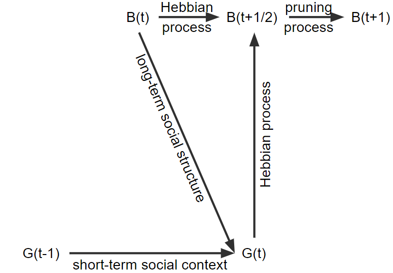
Figure 1: Sketch of the dependencies between the interaction graph $G$ and the social bond graph $B$. Edges having a higher weight in the social bond graph $B(t)$ are more likely to activate, i.e. to be part of the interaction graph $G(t)$. The computation of $B(t+1)$ is done in two steps: first $B$ is updated by the feedback of which edges were active in $G(t)$: unused ties decay while used ties strengthen. The output of this first step is denoted by $B(t+\frac{1}{2})$ because it refers to an intermediary step between $B(t)$ and $B(t+1)$, which is obtained from $B(t+\frac{1}{2})$ by a pruning process, consisting in removing weak unused social ties. The arrow from $G(t-1)$ to $G(t)$ is of a different nature than the arrow from $B(t)$ to $B(t+\frac{1}{2})$. The latter accounts for the inertia of the social bond graph, as $B$ can only encounter gradual change from one time to the next (implementing long-term memory). On the contrary, the arrow from $G(t-1)$ to $G(t)$ does not ensure that $G(t)$ will be similar to $G(t-1)$: it simply describes a short-term social context memory through the fact that the more two nodes share partners in $G(t-1)$, the more likely they are to be partners in $G(t)$.

II.2 Social mechanisms

We use the framework described above to model several social mechanisms.

The first mechanism is a short-term reinforcement process with a long-term memory, through the co-evolution of $G$ and $B$: social agents remember with whom they have interacted and reinforce their social ties with their partners at each interaction, while unused ties weaken. In addition, we assume that weakened ties may vanish: at each timestep $B_{ij}$ has a certain probability to be reset to zero. To capture the realistic assumption that a node tends to shorten unfruitful partnerships to save time or energy, this probability increases as $B_{ij}$ decreases.

The second mechanism we consider is the cyclic closure in the social bond graph $B$. This mechanism captures the fact that, when a social agent initiates a new partnership, it may give the priority to the partners of its partners. Through this mechanism, the existing social bonds drive thus the interactions on $G$.

The third mechanism grasps the fact that two nodes belonging to the same group of discussion are more likely to start interacting together, whether or not they know each other . This can be translated by an increased probability of interaction in $G(t)$ between nodes that were in the same connected component of $G(t-1)$ or, more simply, between nodes that had common neighbors in $G(t-1)$.

The fourth mechanism is a dynamic triadic closure driven by the current context, accounting for the fact that if a node interacts simultaneously with two different nodes, these nodes are likely to also be interacting with each other. It is important to note that this mechanism leads to interactions that are contextual and may thus be of a fundamentally different social significance than intentional ones. In particular, we will take into account that contextual and intentional interactions on $G(t)$ might not influence the evolution of the social bonds in $B$ in the same way.

The four mechanisms are summarized in Figure 2.

II.3 Model implementation

Let us now translate the mechanisms described into microscopic rules of evolution. To this aim, we focus on the AD model in discrete time [30, 20, 21]: each node is endowed with an intrinsic activity parameter $a_{i}$, which gives its probability to be active at each time step. The difference between an active node and an inactive node is that only active nodes can emit intentional interactions.

II.3.1 Creation of the temporal edges of $G(t)$

At each time $t$, each active node $i$ makes $m_{i}$ attempts of intentional interactions, in a way depending on the interactions at the previous time step ($G(t-1)$) and of the current social bond graph ($B(t)$). At each such attempt:

• With probability $p_{g}$, $i$ will extend its egonet, i.e., create an interaction with a node $j$ with whom it has no social bond ($B_{ij}(t)=0$). In this case, $i$ chooses an interaction partner either uniformly at random (with probability $p_{u}$), or, with probability $1-p_{u}$, by triadic closure driven by the social bond graph $B$ (second mechanism above): $i$ creates an interaction in $G(t)$ with a neighbour $j$ of a neighbour $k$ in $B(t)$. Moreover, the choice of $k$ and $j$ are driven by (i) the weights in the social bond graph, $B_{ik}(t)$ and $B_{kj}(t)$, and (ii) the possible existence of a recent common social context (third mechanism). Specifically, the first neighbour $k$ is chosen with probability $P(i\xrightarrow{}k)\propto B_{ik}(t)$, i.e., using the social affinity (independently from a social context). The choice of $j$ as a neighbour of $k$ can be interpreted as a recommendation from $k$ to $i$; therefore, we include here the influence of a social context recently shared by $k$ and $j$, and $j$ is chosen among all neighbours of $k$ with probability:

  $$\tilde{P}(k\xrightarrow{}j)\propto c_{kj}(t-1)B_{kj}(t).$$ (1)

  The coefficient $c_{kj}(t)$ is defined as:

  $$c_{kj}(t)=1+\left|\gamma_{k}(G(t))\cap\gamma_{j}(G(t))\right|\ ,$$ (2)

  representing the boosting of the social affinity by the potential sharing of common neighbours in the previous time step ($\gamma_{\ell}(g)$ denotes the set of neighbours of a node $\ell$ in a graph $g$).

• With probability $1-p_{g}$, $i$ does not extend its egonet, i.e., interacts with one of its neighbours in $B$. This neighbour $j$ is chosen with probability $\tilde{P}(i\xrightarrow{}j)\propto c_{ij}(t-1)B_{ij}(t)$, i.e., proportionally to $i$’s affinity towards $j$, boosted by the potential existence of common neighbours in $G$ at the previous timestep (first and third mechanisms).

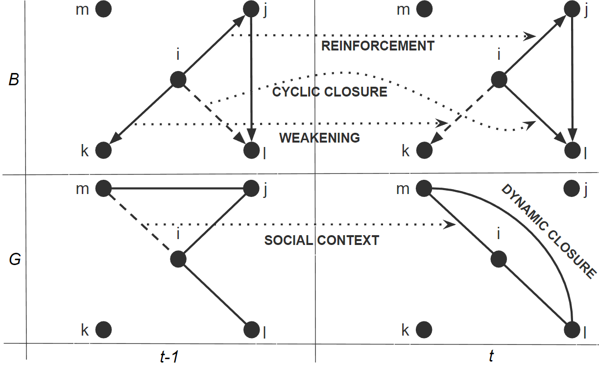
Figure 2: Social mechanisms. We focus on the node $i$ for two consecutive time steps $t-1$ and $t$, so that we do not represent all the ties of $B$. (i) reinforcement: $i$ interacts with $j$ at $t-1$, leading to a reinforcement of the social affinity of $i$ towards $j$: $B_{ij}(t)>B_{ij}(t-1)$. (ii) cyclic closure: at $t-1$, $i$ decides to interact with a new partner. First $i$ picks a known partner $j$ and then a known partner $l$ of $j$. The tie $B_{il}$ is created at $t$. (iii) weakening: while $k$ is part of the egonet of $i$, $i$ does not interact with $k$ at $t-1$. This results in a weakening of the social affinity of $i$ towards $k$: $B_{ik}(t)<B_{ik}(t-1)$. (iv) social context: the social affinity of $i$ towards $m$ at $t$ is temporarily increased by their common partners in $G(t-1)$. (v) dynamic closure: once the intentional interactions have all been drawn at $t$, $(m,i,l)$ is an open triangle in $G(t)$, which is likely to close because $m$ and $l$ are interacting with the same agent.

In addition to these intentional interactions, casual, contextual interactions can occur (fourth mechanism). To take this into account, we implement here a variation of the dynamic triadic closure. Namely, we consider that for each open triangle in $G(t)$ made up of two intentional interactions e.g. $(i,k)$ and $(k,j)$, $i$ and $j$ interact with each other with probability $P_{c}(i,k,j)$ in a contextual, non intentional manner. For the open triangle $(i,k,j)$ to close, either $i$ or $j$ has to propose the contextual interaction. Denoting the probability that $i$ decides to close the triangle by $p_{ij}$, we have:

$$P_{c}(i,k,j)=1-(1-p_{ij})(1-p_{ji})$$ (3)

In our implementation (Fig. 3), $p_{ij}$ takes also into account whether or not $i$ is in the active state: as only active nodes can emit interactions, $p_{ij}=0$ if $i$ is inactive. Moreover, we assume that it depends both on the instantaneous social affinity $b_{ik}$ of $i$ towards $k$ and the instantaneous social affinity $b_{kj}$ of $k$ towards $j$. We define this instantaneous social affinity of a node $\ell$ towards a node $m$ as follows: if $m$ is part of the egonet of $\ell$, then we simply define $b_{\ell m}$ as $\tilde{P}(\ell\xrightarrow{}m)$, i.e. $b_{\ell m}\propto c_{\ell m}(t-1)B_{\ell m}(t)$; if instead $B_{\ell m}$ is zero, we use $b_{\ell m}=p_{g}$ (probability that $\ell$ grows its egonet). We thus use:

$$p_{ij}(t)=\frac{p_{c}b_{ik}(t)b_{kj}(t)c_{ij}(t-1)}{1+p_{c}b_{ik}(t)b_{kj}(t)(c_{ij}(t-1)-1)}$$ (4)

where $0\leq p_{c}\leq 1$ is a free parameter (we use $c_{ij}$ measured at $t-1$ as previously, as it is the social context of the previous time step that influences the link creation at $t$). This form ensures that $p_{ij}$ grows with $p_{c}b_{ik}b_{kj}c_{ij}$ (i.e., is influenced by the social affinities and by the context) and remains between $0$ and $1$.

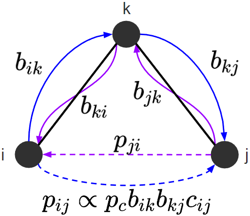
Figure 3: Dynamic triadic closure. After computation of the intentional interactions in $G(t)$, we identify its open triangles. Here $(i,k,j)$ is such an open triangle with edges $(i,k)$ and $(k,j)$ (black straight lines). Closing the triangle means either $i$ decides to interact with $j$ (probability $p_{ij}$), or vice-versa (probability $p_{ji}$). $p_{ij}$ depends both on how close are $i$ and $j$ in the current social context ($c_{ij}$) and how close they are relatively to their common partner of discussion ($b_{ik}$ and $b_{kj}$): if $i$ gives a lot of attention to $k$, and $k$ a lot of attention to $j$, then it is likely that $i$ and $j$ will interact.

II.3.2 Evolution of the social bonds of $B(t)$

The interaction graph at $t$, $G(t)$, is thus composed of the intentional and contextual interactions of all active nodes at $t$. We denote the set of intentional interactions by $I(t)$, and the set of contextual ones by $C(t)$. These interactions determine the change in the social bond graph from time $t$ to the next time step $t+1$. The corresponding update (first mechanism) consists in two steps: a Hebbian-like process and a pruning process. During the Hebbian process, edges of $B(t)$ are either reinforced, weakened or let invariant, according to the rule introduced in [22]: if a node $i$ interacts with $j$ but not $k$, then $B_{ij}$ and $B_{ji}$ may be reinforced, but $B_{ik}$ is weakened (see Figure 4). If $i$ has no interaction at all, its social bonds are not changed.

As a refinement of the reinforcement rule [22], we introduce a distinction between contextual and intentional interactions. To this aim, we denote by $R(t)$ the set of social ties that will be strengthened between $t$ and $t+1$, and by $W(t)$ the set of ties that cannot be weakened (among the ties starting from nodes that have an interaction in $G(t)$, as the nodes with no interaction at $t$ are not affected).

We choose $R$ and $W$ depending on the roles we give to intentional and contextual interactions. A first possibility is to put all interactions on an equal footing: then all active edges are reinforced independently on whether they were intentional or contextual, i.e. $R=W=I\cup C$. If we consider only intentional interactions as relevant, and contextual interactions as noise, then edges from $C$ are not taken into account in the process: $R=W=I$. Finally, if we consider that contextual interactions are neutral, they should give rise neither to a reinforcement nor to a weakening, i.e. $R=I$ and $W=I\cup C$. These possible choices are summarized in Table 1.

Interpretation	$R$	$W$
all interactions are equivalent	$I\cup C$	$I\cup C$
context interactions are neutral	$I$	$I\cup C$
context interactions are noise	$I$	$I$

Table 1: Choices for the update of $B$.

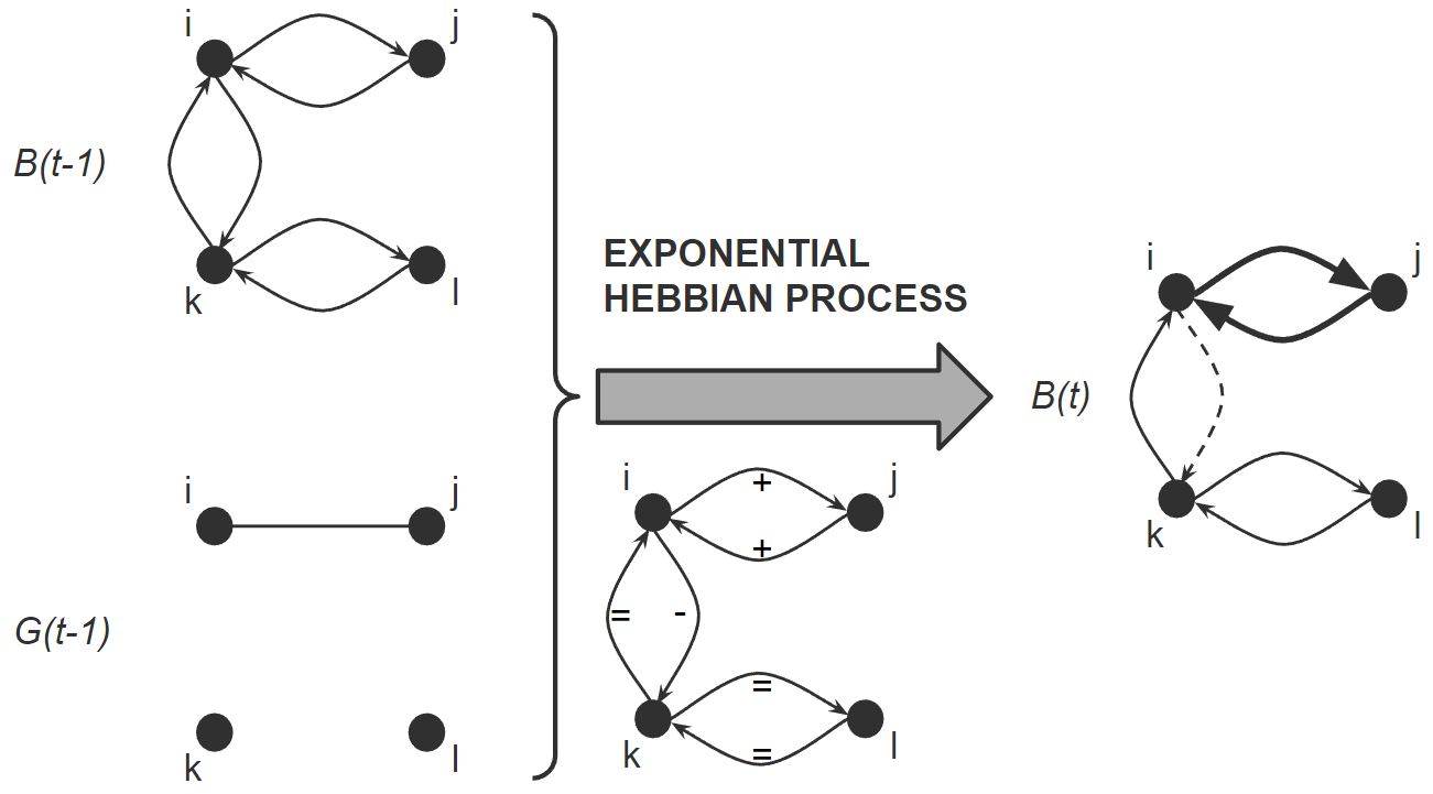
Figure 4: Sketch of the Hebbian-like process describing the evolution of the directed social bond weights from $B(t-1)$ to $B(t)$ due to the interactions in $G(t-1)$. Active edges are reinforced, inactive ties starting from an interacting node are weakened, and ties starting from a non-interacting node are unchanged.

To precisely define the process, we need to specify at which rate a given tie strengthens or weakens. We denote strengthening rates by $\alpha$ and weakening rates by $\beta$. In order to keep the weights of social ties bounded between $0$ and $1$ [22], we also consider rates in $[0,1]$, and we assume them constant. While these rates are also uniform in [22], we consider here that they can be different for different individuals or different ties. We write the general evolution rules as:

$$\forall(i,j)\in R\begin{cases}B_{ij}(t+1)=B_{ij}(t)+\alpha_{ij}(1-B_{ij}(t))\\ B_{ji}(t+1)=B_{ji}(t)+\alpha_{ji}(1-B_{ji}(t))\end{cases}$$ (5)

and:

$$\forall i\in\tilde{R},\forall k,(i,k)\notin R\cup W,B_{ik}(t+1)=(1-\beta_{ik})B_{ik}(t)$$ (6)

where $\tilde{R}$ denotes the set of nodes involved in the links of $R$: $\tilde{R}=\{i|\exists j,(i,j)\in R\}$.

Note that in the original ADM model [21], the social bond weights are not bounded, and simply increase by $1$ at each interaction.

To obtain $B(t+1)$, we include an additional step, namely a pruning of the social bonds, to take into account the fact that weak social bonds might vanish (in the original ADM instead, node disappearance is implemented uniformly at random [21], i.e., with no relation to the actual social bonds).

To quantify how weak is a directed tie $(i,j)$, we compare the probability $P(i\xrightarrow{}j)\propto B_{ij}$ that $i$ selects $j$ among all its neighbours to interact with, with this same probability if all ties starting from $i$ had the same weight. Denoting by $d_{i}^{out}$ the number of out-links of $i$ in $B(t)$, a homogeneous partition of $i$’s interest towards its neighbours would correspond to $P_{hom}(i\xrightarrow{}j)=1/d_{i}^{out}$. Therefore, we use as the probability to remove the directed tie $(i,j)$:

$$\forall i\in\tilde{R},\forall j,(i,j)\notin R\cup W,\\ P_{d}(ij)=\exp\left(-\lambda{d_{i}^{out}}P(i\xrightarrow{}j)\right)$$ (7)

where $\lambda$ is a tunable parameter. $P_{d}(ij)$ is thus large if $P(i\xrightarrow{}j)$ is smaller than its homogeneous counterpart, and decreases exponentially when the importance of $j$ for $i$ increases.

II.3.3 Model versions

Even within the model implementation described in the previous paragraphs, we can define various versions of the model, with for instance different values or distributions of the parameters. Therefore, we first define a baseline version (version V1) with the following features:

• $a_{i}$ is drawn from a power-law of exponent -1 with bounds $a^{\text{min}}$ and $a^{\text{max}}$;

• $m_{i}$ is drawn from a uniform law in $\llbracket 1,m^{\text{max}}\rrbracket$;

• $\alpha_{ij}=\beta_{ij}\equiv\alpha_{i}$ depends only on $i$, and $\alpha_{i}$ is drawn from a power-law of exponent -1 with bounds $0.001$ and $1$;

• the social context at the previous time step is taken into account through $c_{ij}(t-1)=1+\left|\gamma_{i}(G(t-1))\cap\gamma_{j}(G(t-1))\right|$;

• contextual interactions are neutral ($R=I$, $W=I\cup C$, see Table 1);

• the remaining free parameters are: $p_{g}$, $p_{u}$, $p_{c}$, $\lambda$.

We then implement variations with respect to the baseline, by changing in each case only one of the mechanism implementations, as summarized in Table 2. We call these versions adjacent versions, because they differ from the baseline in one aspect only. We tested 12 adjacent versions, numerated from 2 to 13. The version 14 corresponds to the original ADM of [21], with the following properties:

• the egonet growth rate is not constant. Instead of having a fixed probability $p_{g}$ of growing its egonet, each node $i$ grows it with a probability depending on its egonet size: $p_{g}(i)=\frac{c}{c+d_{i}^{out}}$, where $c\in\mathbb{N}$ is a model parameter;

• the recent social context is not taken into account: the direct influence of $G(t-1)$ on $G(t)$ is cut off, i.e. $c_{ij}(t)=1$;

• no contextual interactions are considered, i.e. $p_{c}=0$;

• $B$ has a linear reinforcement process $B_{ij}(t+1)=B_{ij}(t)+1$ for each $(ij)$ in $G(t)$, and weakening of unused social bonds is not considered;

• a node pruning process: instead of removing social ties, we remove social agents with a constant probability $p_{d}$. After removing the social agent $i$, we reinsert it into the system to keep the number of agents constant, but with $B_{ij}=0$ $\forall j$.

This version is thus actually a composite version (i.e., obtained by combining adjacent ones), because it differs from the baseline in more than one aspect.

			version number
			1	2	3	4	5	6	7	8	9	10	11	12	13	14
social mechanisms	social context		Yes	-	-	-	No	-	-	-	-	-	-	-	-	No
	additional interactions		neutral	-	-	-	-	equivalent	noise	None	-	-	-	-	-	None
	egonet growth		constant	-	-	variable	-	-	-	-	-	-	-	-	-	variable
	social bond graph update
	Hebbian process		$\alpha_{i}$	linear	-	-	-	-	-	-	$\alpha$	$\alpha_{i}$, $\beta_{i}$	$\alpha_{ij}$, $\beta_{ij}$	-	-	linear
	$(R,W)$		$(I,I\cup C)$	-	-	-	-	$(I\cup C,I\cup C)$	$(I,I)$	$(I,I)$	-	-	-	-	-	$(I,I)$
	Pruning process		social tie	-	social agent	-	-	-	-	-	-	-	-	-	-	social agent
	$m_{i}$		$\mathcal{U}(\llbracket 1,m^{\text{max}}\rrbracket)$	-	-	-	-	-	-	-	-	-	-	-	constant	constant
	node activity		$a_{i}$	-	-	-	-	-	-	-	-	-	-	$a$	-	-

Table 2: Model versions. The version 1 is the baseline version, while the version 14 is the original ADM. The symbol - means identical to the baseline version. In the row entitled “additional interactions”, we precise the role of the interactions obtained through the dynamic triadic closure mechanism. The indication “None” means that this mechanism does not exist, i.e. $p_{c}=0$. In the row entitled “Hebbian process”, a symbol $\alpha_{i}$ alone means three things. First, the Hebbian process used is an exponential process. Second $\alpha_{ij}=\beta_{ij}=\alpha_{i}$, and third $\alpha_{i}$ is drawn independently for each $i$ from the same power-law of exponent $-1$. Similarly in the row entitled “node activity”, a symbol $a_{i}$ means that $a_{i}$ is drawn from a power-law of exponent -1 independently for each node. On the contrary, an unscripted symbol, like $a$ or $\alpha$, means that the same value is assigned to every node. We put an additional symbol $\beta_{i}$ or $\beta_{ij}$ when the decay rate is drawn independently from the strengthening rate. However, $\alpha_{i}$, $\beta_{i}$, $\alpha_{ij}$, $\beta_{ij}$ are all drawn from power-law distributions with the same exponent -1. In the row titled “$m_{i}$”, the symbol $\mathcal{U}(\llbracket 1,m^{\text{max}}\rrbracket)$ means that $m_{i}$ is drawn independently for each $i$ from the uniform law on the set of integers $\{1,2,\ldots,m^{\text{max}}\}$.

III Comparison with empirical data sets

	name	nodes	timestamps	temporal edges
Conferences	conf16 conf17	138 274	3 635 7 250	153 371 229 536
Schools	utah highschool3	630 327	1 250 7 375	353 708 188 508
Workplace	work2	217	18 488	78 249

Table 3: Sizes of the empirical data sets considered in this paper.

We consider as references several publicly available empirical data sets describing face-to-face interactions in different contexts, namely two scientific conferences, two schools and a workplace (See Table 3 and Supplemental Material, SM). As our aim is to evaluate which hypotheses made on some social mechanisms yield realistic temporal networks, we will thus evaluate how close are the temporal networks $G$ generated by each model version to each reference empirical data set. Note that we compare $G$ and not $B$, as the empirical data sets correspond to instantaneous interactions.

The properties of the temporal networks generated by each model version naturally depend on the version parameters. Some can be extracted or estimated directly from the reference data set: the number of nodes $N$, the duration $T$, and the observed minimum and maximum node activities, $a^{\text{min}}_{\text{obs}}$ and $a^{\text{max}}_{\text{obs}}$. The other parameters are however a priori unknown and tunable. To limit the number of free parameters, we fix the bounds for the power-law followed by the strengthening and weakening rates of the social bonds, $\alpha_{ij}$ and $\beta_{ij}$ (with $\alpha^{\text{min}}=0.001$ and $\alpha^{\text{max}}=1$). The list of remaining free parameters for each model version is given in Table 4.

			related versions	parameter nature	parameter bounds	related mechanisms
free parameters	$p_{u}$		all except $4$ and $14$	probability	$0.001-1$	egonet growth
	$p_{g}$		all except $4$ and $14$	probability	$0.001-1$	egonet growth
	$p_{c}$		all except $4$ and $14$	probability	$0.001-1$	dynamic triadic closure
	$p_{d}$		3,14	probability	$0.001-1$	node pruning
	$a$		12	probability	$a^{\text{min}}_{\text{obs}}-a^{\text{max}}_{\text{obs}}$	interaction proposal
	$a^{\text{min}}$		all except 12	probability	$a^{\text{min}}_{\text{obs}}-a^{\text{max}}_{\text{obs}}$	interaction proposal
	$a^{\text{max}}$		all except 12	probability	$a^{\text{min}}_{\text{obs}}-1$	interaction proposal
	$\alpha$		9	rate	$0.001-1$	Hebbian process
	$\lambda$		all except 3 and 14	intensity	$0.01-10$	edge pruning
	$c$		4,14	integer	$1-4$	egonet growth
	$m$		13,14	integer	$1-4$	interaction proposal
	$m^{\text{max}}$		all except 13 and 14	integer	$1-4$	interaction proposal

Table 4: Free parameters of the models.

Our procedure is thus the following: we first define a set of observables of interest, and a comparison method (a distance) between the outcome of each model version and each reference data set. For each reference and version, we then use a genetic algorithm to find the parameter values minimizing their difference. Note that these optimal parameter values can be different for different references.

For each observable $O$, we can then gather the comparison between each model $M$ and each empirical reference $E$ into a distance tensor $D[\mathcal{O}]_{M,E}$, and subsequently rank all model versions by giving them a score for each observable: the higher the score, the closer the model observable with respect to the empirical ones. Combining the ranks for all observables yields then a global ranking of models.

III.1 Observables

As face-to-face interactions are local in space and time it seems natural to study observables related to small spatio-temporal scales, like nodes, edges or small subgraphs. The simplest observables related to such an object $ob$ are:

• its activity duration: number of consecutive time steps $ob$ exists in the temporal graph;

• its interactivity duration: number of consecutive time steps $ob$ is absent from the temporal graph;

• its aggregated weight: number of times $ob$ has been present in total in the temporal graph;

• its newborn activity: number of consecutive time steps $ob$ exists just after its first occurrence in the temporal graph.

If $ob$ is not a trivial sub-graph like nodes or edges, its size can also be an observable of interest.

Let us now recall some useful definitions:

event:

(see also Figure 5) An event is the combination of an edge $(i,j)$, a starting time $t_{0}$ and a stopping time $t_{f}$ such that $(i,j)$ is inactive at $t_{0}-1$ and $t_{f}+1$, and is active $\forall t$ such that $t_{0}\leq t\leq t_{f}$.

bursty period [18]:

Two events are defined as adjacent if they are defined on the same edge and if the delay between them is less than a given time lapse $\Delta t$. A bursty period is a maximal collection of adjacent events (see Fig. 5).

aggregated network:

The aggregated network on the whole temporal interval $\llbracket 1,T\rrbracket$ is the weighted undirected graph $A$ such that $A_{ij}$ is the aggregated weight of the edge $(i,j)$, i.e., the number of time steps such that $G_{ij}(t)=1$.

aggregation level:

We define the interaction graph aggregated at level $n$, $G^{(n)}$, as follows: $(i,j)\in G^{(n)}(t)\iff(i,j)\in G(\llbracket nt,n(t+1)\llbracket)$. Note that $G^{(n)}$ is unweighted and undirected. We have $G^{(1)}=G$, and $G^{(T)}$ is an unweighted aggregated network on the all temporal interval. Observables of $G^{(n)}$ are called the observables at aggregation level $n$.

Egocentric Temporal Network (ETN) [26, 27]:

An ETN (see Fig. 6) corresponds to a representation of the diversity of the interaction partners of a given node (the ego, in red in Fig. 6) at $d$ consecutive times. In Fig. 6, each ETN reads from left to right (time flow direction). Green circles represent neighbors of the red node. An horizontal edge is drawn between two circles iff they correspond to the same node at different times. The duration of an ETN is called its depth. A $(d,n)-$ETN is an ETN of depth $d$ and aggregation level $n$.

ETN vector:

An ETN vector is a vector $V$ where the component $V_{i}$ is the aggregated weight of the ETN $i$.

We can now define the set of observables we will use to characterize and compare the temporal networks. The observables related to (temporal) subgraphs are (see table 5):

• aggregated weights for edges, (2,1)-ETN and (3,1)-ETN;

• size of connected components of the interaction graph;

• activity and interactivity duration for nodes and edges;

• newborn activity for edges;

• number of events per bursty period (Fig. 5).

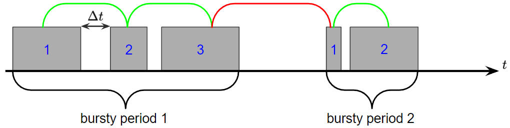
Figure 5: Number of events per bursty period. The sketch represents the activation timeline of a pair of nodes $(i,j)$. A grey rectangle represents an event for $(i,j)$, i.e. a maximal period of uninterrupted interaction between $i$ and $j$. A bursty period is a maximal collection of events that follow each other in time by a delay less than a given threshold, taken here to be 3 time steps. We draw a green junction between two consecutive events if they belong to the same bursty period, i.e. if they are separated by $\Delta t\leq 3$ time steps, and a red junction if $\Delta t>3$. In the example shown, we obtain two distinct bursty periods, with $3$ events in the first and $2$ in the second.

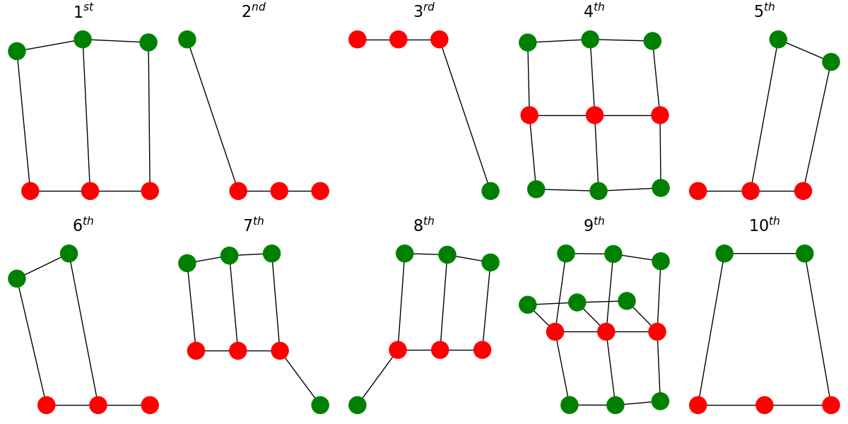
(a) conf16

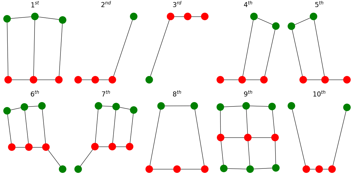
(b) utah

Figure 6: 10 most frequent (3,1)-ETN in two empirical data sets. (a) data set “conf16” (scientific conference), (b) data set “utah” (primary school in Utah). Although those two social contexts are very different their ETNs are quite similar.

		object
		nodes	edges	events	(2,1)-ETN	(3,1)-ETN	connected components of $G(t)$
observable type	aggregated weight		$\times$		$\times$	$\times$
	activity duration	$\times$	$\times$	$\times^{\ast}$
	activity interduration	$\times$	$\times$
	newborn activity		$\times$
	size						$\times$

Table 5: Sub-temporal graph observables. A $(d,n)$-ETN is an ETN of depth $d$ and aggregation level $n$. At the crossing between the row entitled “activity duration” and the column entitled “events”, we wrote an asterisk because the observable we used with events as objects and activity duration as type is called the number of events per bursty period.

In addition, we also consider:

• the clustering coefficient of the aggregated network;

• the degree assortativity in the aggregated network;

• the $(3,n)$-ETN vector including the weights of ETNs computed in the aggregation levels $n$ from 1 to 10: this allows to take into account various timescales in a single observable.

III.2 Comparison method

III.2.1 Distance tensor

We want to quantify how close are a synthetic temporal network and a reference empirical data set, with respect to a given observable. In order to be able to aggregate across observables and obtain a global distance and score, we consider for each observable a distance bounded between 0 and 1. Moreover, we need to consider different metrics for observables for which we have either (i) a distribution (e.g. activity durations or aggregated weights), or (ii) only one numerical value for each network (e.g. the clustering coefficient) or (iii) only one vectorial realization (e.g., ETN vectors).

Point observables.

Let us first consider an observable $\mathcal{O}$ for which we have only one realization per data set $\mathcal{O}(\mathcal{D})\in\mathbb{R}$, where $\mathcal{D}$ is the data set. Then we take as metric:

$$D[\mathcal{O}]_{\mathcal{D},\mathcal{D^{\prime}}}=\frac{|\mathcal{O}(\mathcal{D})-\mathcal{O}(\mathcal{D^{\prime}})|}{2\max(|\mathcal{O}(\mathcal{D})|,|\mathcal{O}(\mathcal{D^{\prime}})|)}$$ (8)

This metric is bounded between 0 and 1, and reaches its maximum value only when $\mathcal{O}(\mathcal{D})=-\mathcal{O}(\mathcal{D^{\prime}})$.

Observables with multiple realizations per data set

If $\mathcal{O}(\mathcal{D})$ is a variable whose distribution $P$ can be sampled, we need to consider a distance between the synthetic and empirical distributions. However $\mathcal{O}(\mathcal{D})$ and $\mathcal{O}(\mathcal{D^{\prime}})$ may yield distributions not equally sampled, possibly on different supports. We choose here to obtain distributions of equal size, by completing the least sampled distribution with zeros, and compare them with the Jensen-Shannon divergence (JSD), which is bounded between 0 and 1. For two discrete distributions $p$ and $q$:

$$\begin{cases}\text{JSD}(p,q)=\frac{1}{2}(\text{KL}(p||m)+\text{KL}(q||m))\\ m=\frac{1}{2}(p+q)\\ \text{KL}(p||m)=\sum_{i}p_{i}\log_{2}(\frac{p_{i}}{m_{i}})\end{cases}$$ (9)

We thus consider the metric:

$$D[\mathcal{O}]_{\mathcal{D},\mathcal{D^{\prime}}}=\text{JSD}(P[\mathcal{O}(\mathcal{D})],P[\mathcal{O}(\mathcal{D^{\prime}})]).$$ (10)

Vector observables.

Now let us consider that $\mathcal{O}(\mathcal{D})\in\mathbb{R}^{d}$, with some $d\in\mathbb{N}$. In our context, this corresponds to the ETN vectors. As we are interested in the relative frequencies of the ETNs, we use the cosine similarity:

$$\text{sim}(\mathcal{O}(\mathcal{D}),\mathcal{O}(\mathcal{D^{\prime}}))=\frac{\mathcal{O}(\mathcal{D})\cdot\mathcal{O}(\mathcal{D^{\prime}})}{||\mathcal{O}(\mathcal{D})||~{}||\mathcal{O}(\mathcal{D^{\prime}})||}.$$ (11)

In fact, in the case of $(3,n)$-ETN, we have a family of $n$ vectors $\{v_{p}\}_{p=1,\cdots,n}$: the $i^{th}$ component of $v_{p}$ is the ratio between the number of occurrences of the motif $i$ at aggregation level $p$ and the number of occurrences of the most frequent motif at aggregation level $p$.

We thus define the similarity between the two families of $n$ vectors as the product of cosine similarities between each pair of vectors at the same level of aggregation:

$$\text{Sim}(v_{1},\ldots,v_{n};v^{\prime}_{1},\ldots,v^{\prime}_{n})=\prod_{p=1}^{n}\text{sim}(v_{p},v^{\prime}_{p}),$$ (12)

and the distance between the two families is $1-\text{Sim}$.

III.2.2 From distances to a score

Our goal is to understand which model versions are best able to reproduce empirical properties observed in a series of data sets. For each model version, and each observable, we thus define a score by comparing the minimal distances between synthetic and empirical data with the distance between empirical data sets themselves. To this aim, given an observable $\mathcal{O}$ and a model version $\mathcal{V}$, we:

1. compute for each empirical data set $\mathcal{E}$ its distance $\delta[\mathcal{O}]_{\mathcal{V},\mathcal{E}}$ to the set of model instances, i.e., the minimal distance $\min_{\mathcal{D}}D[\mathcal{O}]_{\mathcal{D},\mathcal{E}}$ over all instances $\mathcal{D}$ of the model $\mathcal{V}$;

2. compute the median of the distances between $\mathcal{V}$ and all empirical data sets:

   $$m^{\text{inter}}_{\mathcal{O}}(\mathcal{V})=\text{median}(\delta[\mathcal{O}]_{\mathcal{V},\mathcal{E}})$$ (13)

   where the index $\mathcal{E}$ runs over the empirical data sets;

3. compute the characteristic distance between empirical data sets themselves:

   $$m^{\text{intra}}_{\mathcal{O}}=\text{median}(D[\mathcal{O}]_{\mathcal{E},\mathcal{E^{\prime}}})$$ (14)

   where the indices $\mathcal{E},\mathcal{E^{\prime}}$ both run over the empirical data sets ($\mathcal{E}\neq\mathcal{E^{\prime}}$);

4. compute the interquartile range of distances between empirical data sets, $Q_{3}-Q_{1}$;

5. deduce the score of the model version $\mathcal{V}$ for observable $\mathcal{O}$:

   $$\text{score{\hbox{_\mathcal{O}}}({\hbox{\mathcal{V}}})}=\frac{m^{\text{intra}}_{\mathcal{O}}-m^{\text{inter}}_{\mathcal{O}}(\mathcal{V})}{Q_{3}-Q_{1}}.$$ (15)

This procedure is illustrated in Fig. 7. A higher score corresponds to the fact that the model version has instances with statistical properties closer to the empirical ones, for the chosen observable.

Note that, while this procedure is intended to provide a score to models, we can also apply it also to each empirical data set. The interpretation is then not a “score”, but quantifies how close a data set is to the other ones.

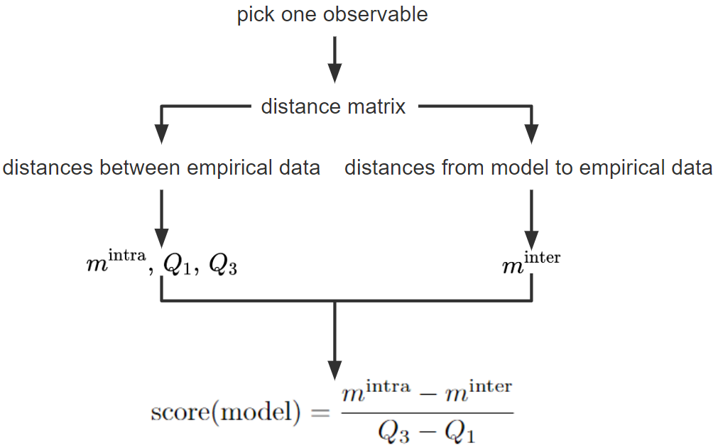
Figure 7: Computing the score of a model. The evaluated data sets consist in all versions of the models presented in Table 2 and the empirical data sets presented in Table 3. For each data set, a different score is computed for each observable. The higher the score of a model, the closer the distribution of the associated observable is from the distributions in the empirical data sets. Said otherwise, a higher score means more realistic statistical properties for the associated observable.

III.3 Results

We first illustrate that our approach providing a score using the proximity tensor is compatible with a qualitative direct appreciation of the distributions. We then detail the genetic tuning of the free parameters. This allows us to identify the best model belonging to the class investigated here. We then investigate in more details the interplay between observables and the role of each mechanism in our model, i.e., which observables change when a given mechanism or hypothesis is changed.

III.3.1 Illustration

Figure 8 displays the distribution of several observables for two empirical data sets corresponding to different contexts and three model versions. This illustrates how, for each observable that can be sampled, a higher score is associated with a distribution closer to the empirical ones.

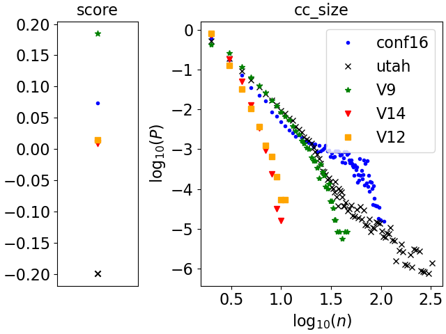
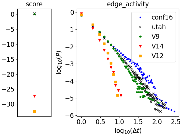
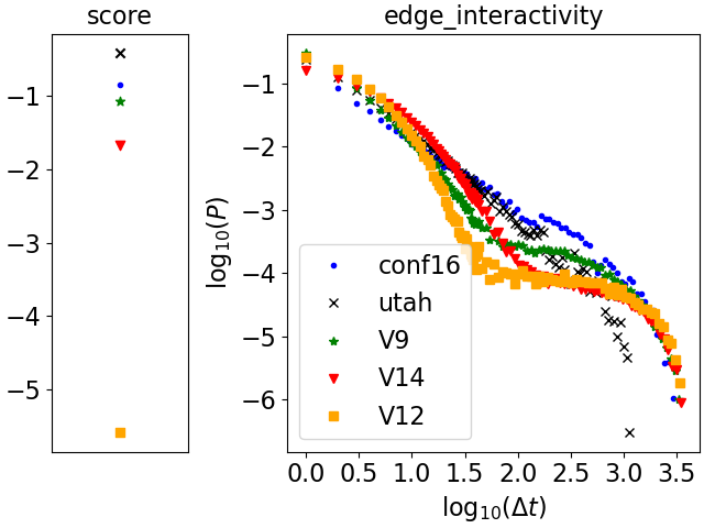
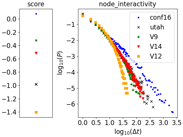
Figure 8: Illustration of the scores for several observables and models. The figure displays in each panel the distribution of an observable (”cc_size”: size of connected components) for two data sets (the conference “conf16” and the school “utah”) and three model versions: the original ADM (V14), the adjacent version with the highest average score (V9) and the version with the lowest average score (V12). The three models were optimized with respect to the “utah” reference. The score is computed in each case by Eq. 15: a higher score is associated with a distribution closer to the empirical one. In the top left panel, “utah” has a low score because the “cc_size” observable is the only distribution which is not similar for all empirical references.

For point observables (the clustering coefficient and degree assortativity of the fully aggregated network), the score associated with a point observable does not necessarily reflect the degree of proximity with an empirical reference (not shown): this is due to the fact that these point observables are highly variable from one empirical data set to another.

It is more difficult to check the accordance between a high score for the ETN vector observable and realistic motifs because we can visualize only a few motifs. As an illustration however, we display in Fig. 9(a) the five most frequent motifs at aggregation level $5$ of the “utah” data set and the instances associated with this reference of the models with highest and lowest ETN scores. The “utah” instance of the version with the highest ETN score has exactly the same 5 most frequent (3,5)-ETN as the “utah” reference, while this is not the case of the instance of the version with the lowest score.

Figure 9(d) moreover shows the ETN autosimilarity for three model versions and two references. We define the ETN autosimilarity of a data set at a given depth $d$ and aggregation level $n$ as the ETN similarity (defined in III.2.1) between the $(d,n)$- and $(d,1)$-ETN vectors of this data set. The empirical references are highly autosimilar, i.e. their ETN autosimilarity is close to $1$ for various levels of aggregation. We also display in the figure the ETN autosimilarity of three model versions (V9, V12 and V14), using in each case the instance tuned to be as close as possible to the reference “utah”. The higher the score of a model version, the closer its ETN autosimilarity curve to the “utah” reference.

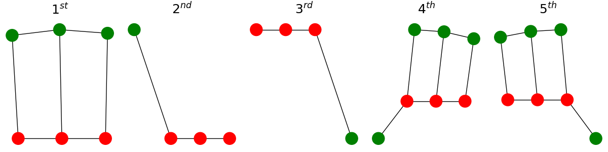
(a) best adjacent version

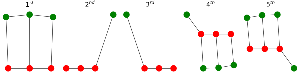
(b) empirical reference ’utah’

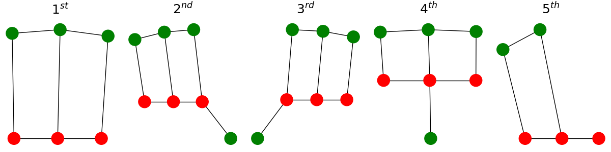
(c) worst adjacent version

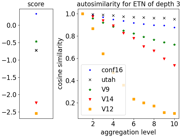
(d) ETN autosimilarity

Figure 9: Interpretation of the score of the ETN vector observable. Fig 9(a), 9(b), 9(c): Five most frequent ETN of depth 3 at aggregation level 5 for two models tuned w.r.t. the empirical reference “utah”. The model with the highest score (V9) has the same motifs as the reference, but not the worst version (V12). Fig 9(d): ETN autosimilarity for three models (the best V9, the worst V12 and the original ADM V14) and two empirical references. The ETN autosimilarity of a given data set at aggregation level $n$ is the cosine similarity between the motifs observed in this data set at level $n$ and the motifs observed in this data set at level $1$. Empirical references are highly autosimilar with respect to this measure. For models, a higher score for the ETN vector corresponds to a higher ETN autosimilarity.

III.3.2 Tuning the models’ parameters by a genetic algorithm

For each model version and each reference data set, we want to obtain the parameter values that yield temporal networks instances as close as possible to the reference. Recall that given a reference data set and a model version, there are three types of parameters: (i) frozen parameters that depend only on the version, like the bounds for the power-laws of strengthening and decay rates $\alpha_{ij}$, $\beta_{ij}$; (ii) readable parameters that depend only on the reference, like $N$, $T$, $a^{\text{min}}_{\text{obs}}$ and $a^{\text{max}}_{\text{obs}}$; (iii) free parameters, that depend both on the version and the reference, that we tune to get as close as possible to the reference data set, e.g., $p_{c}$ or $m^{\text{max}}$ (see Table 4 for the list of parameters).

To tune the free parameters, we use a genetic algorithm (described in the SM), with a fitness set to the distance between the reference data set and the instance of the temporal network generated by the model. However, computing the distances for all observables is computationally costly while, in a genetic algorithm, the fitness computation should be fast as it is computed at each iteration and for each genetic sequence. Therefore, we choose here to use as fitness only the distance relative to the ETN vector with the first ten levels of aggregation, i.e. the $(3,n)$-ETN for $n=1,\ldots,10$. This observable is indeed computationally efficient and covers various time and spatial scales.

We find that this is enough for the model to improve on other observables too: we illustrate this point in the SM by comparing random instances with tuned instances along several observables. Some distributions remain different from their empirical counterparts, in particular the distributions of sizes of connected components (“cc_size”), which however differ also between data sets. A better agreement and better scores might be obtained at the cost of an increased computational effort, by including additional features in the genetic algorithm fitness. Overall, how to keep the computational effort of the genetic algorithm low while obtaining a good similarity between model and data statistics on a large range of observables remains an open interesting question. We have also checked that the fitness is positively correlated with the score of every observable, which means that, despite these limitations, the genetic tuning does what it was intended to: obtain instances with closer statistical properties from empirical references than random instances in every observable. In the SM, we also investigate how the values of the tuned parameters are distributed across versions and references.

III.3.3 Most realistic model within the ADM class

To compare the models, we first compute for each observable a ranking of the model versions using their score, computed using the distances between each instance obtained by the genetic tuning and the corresponding reference data set. To then determine the best model among the 14 versions presented above, it is necessary to define a global score for each model version. We consider two possible strategies:

• the global score of a model (or data set) is given by its rank averaged over all observables;

• the global score of a model (or data set) is given by its score summed over all observables and the global rank is just the rank according to the global score.

Note that other global ranks could be obtained by attributing different weights to the score or rank for different observables. We choose here however not to favor an observable over another. The resulting rankings are shown on Figure 10. The original ADM performs very low in both rankings, and the two best versions are the baseline version and the version 9, i.e. with $\alpha_{ij}=\beta_{ij}=\alpha$. We also show in the SM the rankings of all model versions for each observable separately: despite a rather large variability between rankings, the baseline version remains within the five first ranks for 6 observables, and the version 9 for 8 observables.

In the next subsections, we investigate this global result in more details, to understand in particular how each model performs with respect to each observable, and the impact of the various mechanisms on the models’ performances.

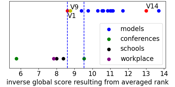
(a) averaging the ranks

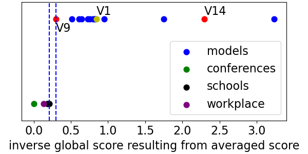
(b) averaging the scores

Figure 10: Global ranking of the models 1 to 14 according to two possible ranking strategies. In each panel, the $y$ coordinate is arbitrary: empirical data sets have been placed at $y=0$ while artificial data sets are aligned at $y=1$. The global ranking is obtained by sorting the models by increasing order of the $x$ coordinate (hence “inverse global score”). In each panel, the best version as well as the original ADM are highlighted as red dots. The best version in the other ranking strategy is displayed as a yellow dot. Blue vertical dashed lines indicate either the crossover or the gap between empirical and artificial data sets. (a): The $x$-coordinate is given by the model rank averaged over all observables. The best version is the baseline V1, almost ex aequo with version 9. (b) the $x$-coordinate is given by the opposite of the averaged score, shifted by the maximum averaged score to take positive values. Version 9 ($\alpha_{ij}=\beta_{ij}=\alpha$) is here the best one. In both panels, the original ADM is ranked rather low. There is either an overlap (a) or a small gap (b) between models and empirical data sets. Thus the class of models considered here is able to generate synthetic data sets with statistical properties close from real data sets.

III.3.4 Similarity between observables

First, we need to investigate the fact that the observables we have chosen to characterize our social temporal networks are not independent. In particular, when modifying a modeling hypothesis or a parameter value, several observables may be modified in a correlated way. Understanding these correlations can help better interpret the effect of varying the modeling hypotheses. We thus define a similarity between two observables as the Kendall tau between the rankings of the models using these observables. The resulting similarity matrix between observables is shown in Fig. 11. We then extract groups of correlated observables by converting this matrix into a weighted undirected network: the nodes of this network are the observables and the weight $w_{\mathcal{O}\mathcal{O^{\prime}}}$ is the absolute value of the Kendall similarity between rankings of observables $\mathcal{O}$ and $\mathcal{O^{\prime}}$. The network is shown in Fig. 11, on which we use the community detection algorithm of the software Gephi [37], based on modularity maximization, to obtain the three following groups:

• group I (blue): node activity interduration, edge weight, size of connected components, ETN vector and (2,1)-ETN weight;

• group II (orange): node, edge and newborn edge activity duration, degree assortativity and (3,1)-ETN weight;

• group III (green): edge activity interduration, events activity duration and clustering coefficient.

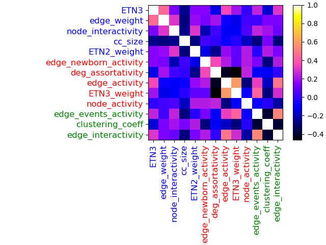
(a) Similarity matrix between observables

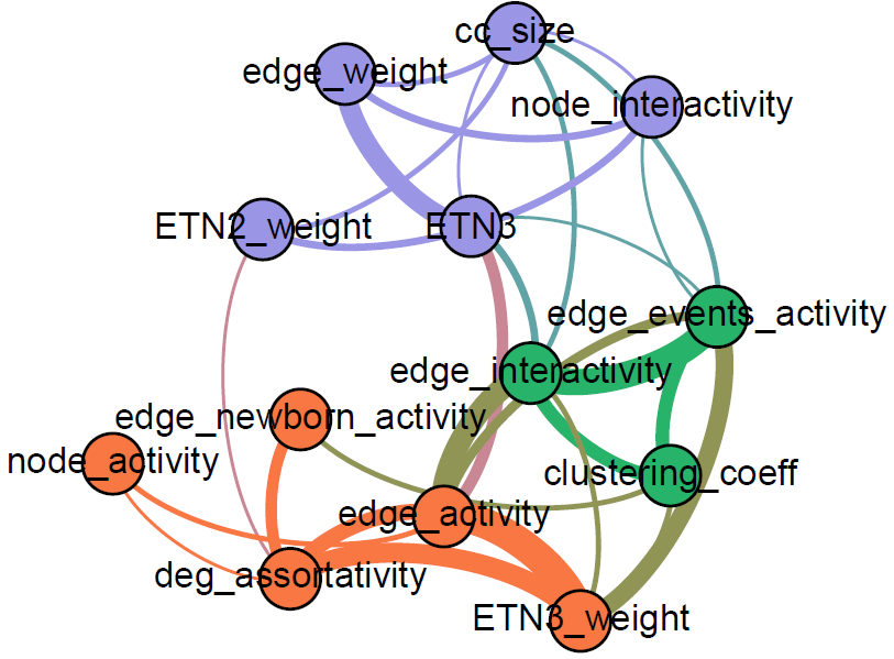
(b) Similarity network of observables

Figure 11: Similarity between observables. (a) Similarity matrix obtained by computing the Kendall similarity between the associated rankings of our model versions (note that the results might be different if considering a different ensemble of models). The observables are quite independent from each other (low absolute values for the similarity for almost all observables pairs). Strong negative couplings are observed only between the point observables and some distribution observables. The ETN vector is either positively or weakly coupled to every other observable, in accordance with the conclusion of III.3.2: improving on motifs generally means improving on other observables. (b) The matrix is turned into a weighted network by taking as edge weight the absolute value of the Kendall similarity. A community detection algorithm based on modularity optimization detects three groups of observables (colored according to the group they belong to). The thickness of an edge is proportional to its weight and we filter out small weights for visualization purposes.

III.3.5 Impact of hypotheses on model performances

In order to have more precise information about how hypotheses impact each observable, depending on the group it belongs to, we define for each model version its score relative to a group of observables as follows:

1. for each observable in the group (I, II or III), we compute the score of the model version as well the score of the baseline version V1;

2. we compute the difference between the score of the version and the score of the baseline version;

3. we sum the differences obtained for each observable in the group.

Figure 12 shows the resulting group scores for the various versions. We also indicate the relative contribution of each observable inside the group to the group score. Finally, we summarize in Table 6 which hypotheses lead to an improvement or a worsening with respect to the baseline version.

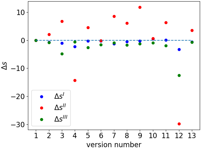
(a) Score variation for each group of observables

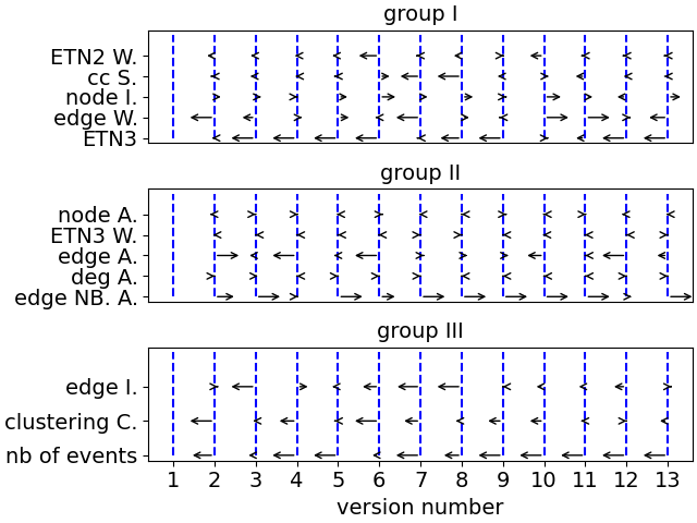
(b) Contribution of each observable to each group score

Figure 12: Score variation resulting from the change of hypothesis with respect to the baseline model. For each version, we compute the difference between its score and the score of the baseline (V1). In panel 12(a), these differences are summed over all observables of each of the groups identified in Fig. 11. The sum over group I (resp. II, III) is called the score I (resp. II, III) and is denoted by $\Delta s^{\text{I}}$ (resp. $\Delta s^{\text{II}}$, $\Delta s^{\text{III}}$). (a): Score differences for each adjacent model version. Blue dots correspond to scores I, red dots to scores II and green dots to scores III. The horizontal dashed line indicates the line of no changes in score. (b): Differences in score for each observable, represented as horizontal arrows. A difference is positive when the arrow points to the right and negative when it points to the left. Vertical blue dashed lines correspond to $\Delta s=0$. The arrow length is proportional to the difference in score, rescaled so that the longest arrow spans an arbitrary length of $0.5$ unit. The edge weight and the size of connected components (cc_size) are the only observables on which a significant improvement is observed with respect to the baseline version.

n	difference with version 1	$\Delta s^{\text{I}}$	$\Delta s^{\text{II}}$	$\Delta s^{\text{III}}$
2	linear process	0	+	0
3	node pruning	0	+	-
4	varying egonet growth	-	-	0
5	$c_{ij}(t)=1$	0	+	-
6	$R=W=I\cup C$	0	0	-
7	$R=W=I$	0	+	0
8	$p_{c}=0$	0	+	0
9	$\alpha$	0	+	0
10	$\alpha_{i}$, $\beta_{i}$	0	0	0
11	$\alpha_{ij}$, $\beta_{ij}$	0	+	-
12	$a$	-	-	-
13	$m$	0	+	0

Table 6: Outcome of hypotheses on the sign of the three group scores. For each version, we indicate the sign of scores I, II and III. Many versions have a score similar to the basis version. Improvement is only observed for group II, and comes often with a loss over the two other groups.

Figure 12(a) indicates that the baseline version seems to be optimal for observables from group I and III, since no version exhibits improvement on either group. However, 8 out of 12 adjacent versions show an improvement for group II. The most common signature is $0,+,0$: 5 versions show no change on groups I and III and an improvement on group II.

In terms of mechanisms, updating the social bond graph with a linear Hebbian process with no decay (V2) improves over the exponential Hebbian process of the baseline version, but if we use an exponential Hebbian process with a uniform value $\alpha_{ij}=\beta_{ij}=\alpha$ (V9), then we get still better results. Thus, in order to recover a more realistic social system, agents should all update their social ties in the same way, i.e. with the same homogeneous parameter $\alpha$. The observation for the intrinsic activity $a_{i}$ is the opposite: imposing a uniform value $a_{i}=a$ (V12) leads to a drastic loss in score for all groups. Heterogeneity in the intrinsic activities seems to be necessary to recover a realistic social system. On the other hand, a uniform number of emitted interactions (V13) leads to an improvement. Actually (see SM), the value for $m$ or $m^{\text{max}}$ returned by the genetic tuning is $1$ in most cases: a higher value probably causes the nodes to have a too large instantaneous degree, i.e. agents interact with more other agents than what is realistic, leading to unrealistic ETN motifs.

Figure 12(a) also yields interesting insights concerning the update of the social bond graph and the contextual interactions. A uniform node pruning (V3) leads to poor performance on group III observables quite as equivalent as the gain over group II. Not taking into account the social context, i.e. putting $c_{ij}=1$ (V5) also leads to opposite changes: we gain over group II and loose over group III. Regarding contextual interactions, considering them leads to a significant improvement under the condition that they are treated as pure noise (V7). Having no contextual interaction at all (V8) also leads to an improvement, but of smaller amplitude. Thus adding noise in our system makes it more realistic, which can be understood by the fact that many interactions have in fact little social significance and occur only due to context.

Figure 12(b) gives more detailed information by indicating the relative contribution of each observable to the group score. In particular, some observables always give a negligible contribution to the score of the group they belong to. This is in part due to the fact that some observables are shared across all versions, i.e. their realizations are similar in all versions. This is the case of “ETN2 weight” and “ETN3 weight”, whose distribution always match almost perfectly the empirical case (after genetic tuning).

Other observables are shared across almost all versions, like “node activity” and “node interactivity”, which are similar for all versions except version 12, characterized by $a_{i}=a$ (however, for this version the loss in score relatively to those two observables is negligible compared to the loss relative to the other ones).

Overall, the 8 major observables, which are mainly responsible for the observed group scores, are:

• in the group I: “size of connected components”, “edge weight”, “ETN3”

• in the group II: “edge activity”, “edge newborn activity”

• in the group III: “edge interactivity”, “clustering coeff”, “edge events activity”

All observables relative to edges are major observables. However, the fact that an observable contributes a lot to the score of its group does not mean that it is necessarily relevant: as the point observables are not shared across empirical references, we must be careful when we score a model relatively to them. For instance, if we considered that only relevant observables should be robust over empirical social systems, then the clustering coefficient and the degree assortativity should not be used to score and rank models. Why some observables contribute more than others might also depend on how shared they are between references: if an observable has almost the exact same realizations in every empirical reference, then the associated interquartile range will be almost zero, which can lead to high variations in the score for models (cf. Eq. 15).

It is finally important to note that, except for the original ADM (V14), the model versions considered differ from the baseline version by one hypothesis only. The question arising naturally is the following: if we accumulate modifications with respect to the baseline version, do variations in score accumulate accordingly? If so, Table 6 could be used to design even more realistic models by combining the hypotheses that lead to improvements: for each mechanism, we can check whether the variation from the baseline leads to an improvement or not, and combine the variations that do. We explore this avenue in the SM for several composite versions. The relation between the score of a composite version and the scores of its adjacent components is however non trivial, and the best version remains V9 even when taking into account the composite versions.

IV Discussion

In this paper, we have presented a general framework allowing to design various models by controlling their qualitative aspects. We have considered a modeling framework based on the idea of a co-evolution of an observed interaction network and an underlying and unobserved social bond network. Within the overall framework of the activity driven model with memory [30, 21], we hypothesized that social bonds partially drive the observed interactions, together with an influence of the current social context, and that interactions impact social bonds [22]: the corresponding strengthening and weakening of social bonds take into account the fact that an interaction reinforces a social bond, and that resources (time, energy) are needed to maintain a social bond, so that the absence of interaction weakens it. Instead of the usual exploration of a parameter space for a given set of mechanisms, we have then considered, within this framework, an exploration of a hypotheses space, corresponding to representations of several possible social mechanisms. Parameters corresponding to each hypothesis are then tuned by a genetic algorithm to maximize the similarity between model instances and a given empirical data set. While such similarity can be defined a priori in many ways, we find that using only the ETN vector to quantify it and tune the parameters leads to an improvement for many other observables, indicating that many statistical properties of a social temporal network are related to its ETN motifs [27]. We recall that the ETN vector is given by the list and frequencies of ETN motifs at various levels of aggregation (1 to 10 in our case), which thus encodes several spatiotemporal scales. This procedure allows us to define a score for each model, relative to each observable considered and globally, and to deduce which mechanisms lead to more realistic artificial temporal networks. In particular, many of the model versions considered perform better than the original Activity Driven model with memory. Once tuned, each model version can produce synthetic data sets of arbitrary sizes and durations and with realistic properties, which can be used for instance as support for numerical simulations of dynamical processes on temporal networks.

Our work entails a number of limitations that are worth discussing. First, the list of observables we consider to rank models is somewhat arbitrary: we investigated observables of different types (point, with multiple realizations, vector) and dealing with various scales, but other observables could be thought of, while some might be removed from the list because of their variability among the empirical references (e.g., clustering coefficient). Second, the scoring mechanism may also be improved. Indeed, a higher score is not always clearly associated with a value of the observable closer to the empirical value. Future work will thus address the issue of building another ad hoc score measure with a clearer interpretation.

The use of a series of statistical properties to determine whether a model is producing realistic temporal networks can also be discussed. Indeed, empirical data sets show large activity variations, i.e., in the number of interactions per timestamp. These variations can be driven by changes in population size or in intrinsic activity [38], either due to imposed schedules or to spontaneous bursts. Such patterns cannot be recovered in the class of models we have explored, for which the number of interactions per timestamp is stationary with small fluctuations. Exploring other classes of models would be necessary to account for the large empirical variations. The methodology considered in this paper could however then still be used to cover such extended classes. In particular, our results suggest that the full exploration of the hypotheses space is not necessary, as properties of composite models could be predicted from their adjacent components.

Despite these limitations, the partial exploration we performed allowed to determine models with a much higher degree of realism than the original ADM, and also to show the interest of modeling several social mechanisms such as taking into account the social context, considering casual interactions (dynamic triadic closure) and updating the underlying social bond ties through an exponential Hebbian process with both strengthening and weakening mechanisms. The class of models we have considered could also be extended, e.g. by adding group memberships, or by considering various types of Hebbian processes: delayed or anti-Hebbian process, or allowing negative interactions and possibly negative social bonds [34, 35].

References

- Granovetter [1973] M. S. Granovetter, The strength of weak ties, American Journal of Sociology 78, 1360 (1973).
- Hinde [1976] R. A. Hinde, Interactions, relationships and social structure, Man 11, 1 (1976).
- Wasserman and Faust [1994] S. Wasserman and K. Faust, Social network analysis: Methods and applications, Vol. 8 (Cambridge university press, 1994).
- Mossong et al. [2008] J. Mossong, N. Hens, M. Jit, P. Beutels, K. Auranen, R. Mikolajczyk, M. Massari, S. Salmaso, G. S. Tomba, J. Wallinga, J. Heijne, M. Sadkowska-Todys, M. Rosinska, and W. J. Edmunds, Social contacts and mixing patterns relevant to the spread of infectious diseases, PLoS Med 5, e74 (2008).
- Conlan et al. [2011] A. J. K. Conlan, K. T. D. Eames, J. A. Gage, J. C. von Kirchbach, J. V. Ross, R. A. Saenz, and J. R. Gog, Measuring social networks in british primary schools through scientific engagement, Proceedings of the Royal Society B: Biological Sciences 278, 1467 (2011).
- Malik [2018] M. M. Malik, Bias and beyond in digital trace data, Ph.D. thesis, Doctoral dissertation, Carnegie Mellon University (2018).
- Schaible et al. [2021] J. Schaible, M. Oliveira, M. Zens, and M. Génois, Sensing close-range proximity for studying face-to-face interaction, in Handbook of Computational Social Science, Volume 1 (Routledge, 2021) pp. 219–239.
- Cattuto et al. [2010] C. Cattuto, W. Van den Broeck, A. Barrat, V. Colizza, J.-F. Pinton, and A. Vespignani, Dynamics of person-to-person interactions from distributed rfid sensor networks, PLoS ONE 5, e11596 (2010).
- Salathé et al. [2010] M. Salathé, M. Kazandjieva, J. W. Lee, P. Levis, M. W. Feldman, and J. H. Jones, A high-resolution human contact network for infectious disease transmission, Proceedings of the National Academy of Sciences 107, 22020 (2010).
- Stehlé et al. [2011] J. Stehlé, N. Voirin, A. Barrat, C. Cattuto, L. Isella, J.-F. Pinton, M. Quaggiotto, W. Van den Broeck, C. Régis, B. Lina, et al., High-resolution measurements of face-to-face contact patterns in a primary school, PloS one 6, e23176 (2011).
- Barrat et al. [2013] A. Barrat, C. Cattuto, V. Colizza, F. Gesualdo, L. Isella, E. Pandolfi, J.-F. Pinton, L. Ravà, C. Rizzo, M. Romano, et al., Empirical temporal networks of face-to-face human interactions, The European Physical Journal Special Topics 222, 1295 (2013).
- Stopczynski et al. [2014] A. Stopczynski, V. Sekara, P. Sapiezynski, A. Cuttone, M. M. Madsen, J. E. Larsen, and S. Lehmann, Measuring large-scale social networks with high resolution, PLoS ONE 9, e95978 (2014).
- Toth et al. [2015] D. J. Toth, M. Leecaster, W. B. Pettey, A. V. Gundlapalli, H. Gao, J. J. Rainey, A. Uzicanin, and M. H. Samore, The role of heterogeneity in contact timing and duration in network models of influenza spread in schools, Journal of The Royal Society Interface 12, 20150279 (2015).
- Sapiezynski et al. [2019] P. Sapiezynski, A. Stopczynski, D. D. Lassen, and S. Lehmann, Interaction data from the copenhagen networks study, Scientific Data 6, 315 (2019).
- Holme [2015] P. Holme, Modern temporal network theory: a colloquium, The European Physical Journal B 88, 1 (2015).
- Holme and Saramäki [2012] P. Holme and J. Saramäki, Temporal networks, Physics reports 519, 97 (2012).
- Stehlé et al. [2010] J. Stehlé, A. Barrat, and G. Bianconi, Dynamical and bursty interactions in social networks, Physical review E 81, 035101 (2010).
- Karsai et al. [2012] M. Karsai, K. Kaski, A.-L. Barabási, and J. Kertész, Universal features of correlated bursty behaviour, Scientific Reports 2, 397 (2012).
- Vestergaard et al. [2014] C. L. Vestergaard, M. Génois, and A. Barrat, How memory generates heterogeneous dynamics in temporal networks, Phys. Rev. E 90, 042805 (2014).
- Karsai et al. [2014] M. Karsai, N. Perra, and A. Vespignani, Time varying networks and the weakness of strong ties., Sci Rep 4, 4001 (2014).
- Laurent et al. [2015] G. Laurent, J. Saramäki, and M. Karsai, From calls to communities: a model for time-varying social networks, The European Physical Journal B 88, 10.1140/epjb/e2015-60481-x (2015).
- Gelardi et al. [2021] V. Gelardi, D. Le Bail, A. Barrat, and N. Claidiere, From temporal network data to the dynamics of social relationships, Proceedings of the Royal Society B 288, 20211164 (2021).
- Jo et al. [2011] H.-H. Jo, R. K. Pan, and K. Kaski, Emergence of bursts and communities in evolving weighted networks, PloS one 6, e22687 (2011).
- Kumpula et al. [2007] J. M. Kumpula, J.-P. Onnela, J. Saramäki, K. Kaski, and J. Kertész, Emergence of communities in weighted networks, Physical review letters 99, 228701 (2007).
- Orsini et al. [2015] C. Orsini, M. M. Dankulov, P. Colomer-de Simón, A. Jamakovic, P. Mahadevan, A. Vahdat, K. E. Bassler, Z. Toroczkai, M. Boguñá, G. Caldarelli, S. Fortunato, and D. Krioukov, Quantifying randomness in real networks, Nature Communications 6, 8627 (2015).
- Longa et al. [2022a] A. Longa, G. Cencetti, B. Lepri, and A. Passerini, An efficient procedure for mining egocentric temporal motifs, Data Mining and Knowledge Discovery 36, 355 (2022a).
- Longa et al. [2022b] A. Longa, G. Cencetti, S. Lehmann, A. Passerini, and B. Lepri, Neighbourhood matching creates realistic surrogate temporal networks, arXiv , arXiv:2205.08820 (2022b).
- Dunbar et al. [2009] R. I. Dunbar, A. H. Korstjens, J. Lehmann, and B. A. C. R. Project, Time as an ecological constraint, Biological Reviews 84, 413 (2009).
- Miritello et al. [2013] G. Miritello, R. Lara, M. Cebrian, and E. Moro, Limited communication capacity unveils strategies for human interaction, Scientific reports 3, 1 (2013).
- Perra et al. [2012] N. Perra, B. Gonçalves, R. Pastor-Satorras, and A. Vespignani, Activity driven modeling of time varying networks., Scientific reports 2, 469 (2012).
- Ubaldi et al. [2016] E. Ubaldi, N. Perra, M. Karsai, A. Vezzani, R. Burioni, and A. Vespignani, Asymptotic theory of time-varying social networks with heterogeneous activity and tie allocation, Scientific Reports 6, 35724 (2016).
- Thurner [2018] S. Thurner, Virtual social science, arXiv preprint arXiv:1811.08156 (2018).
- Ilany et al. [2013] A. Ilany, A. Barocas, L. Koren, M. Kam, and E. Geffen, Structural balance in the social networks of a wild mammal, Animal Behaviour 85, 1397 (2013).
- Gelardi et al. [2019] V. Gelardi, J. Fagot, A. Barrat, and N. Claidière, Detecting social (in)stability in primates from their temporal co-presence network, Animal Behaviour 157, 239 (2019).
- Andres et al. [2022] G. Andres, G. Casiraghi, G. Vaccario, and F. Schweitzer, Reconstructing signed relations from interaction data, arXiv , arXiv:2209.03219 (2022).
- Note [1] Note that this is different from focal closure, which suggests the formation of ties between individuals with common attributes or interests, and which is implemented by links with randomly chosen individuals in [21].
- Bastian et al. [2009] M. Bastian, S. Heymann, and M. Jacomy, Gephi: an open source software for exploring and manipulating networks, in Proceedings of the international AAAI conference on web and social media, Vol. 3 (2009) pp. 361–362.
- Kobayashi and Génois [2020] T. Kobayashi and M. Génois, Two types of densification scaling in the evolution of temporal networks, Phys. Rev. E 102, 052302 (2020).