On the Statistical Consistency of a Generalized Cepstral Estimator

Abstract

We consider the problem to estimate the generalized cepstral coefficients of a stationary stochastic process or stationary multidimensional random field. It turns out that a naive version of the periodogram-based estimator for the generalized cepstral coefficients is not consistent. We propose a consistent estimator for those coefficients. Moreover, we show that the latter can be used in order to build a consistent estimator for a particular class of cascade linear stochastic systems.

I Introduction

Given a stationary time series $y_{0},y_{1},\dots,y_{N-1}$, the estimation of some second-order statistics of the series, e.g., the covariances $c_{k}:={\mathbb{E}}\,[y_{t+k}\,y_{t}^{*}]$ where ${\mathbb{E}}$ denotes mathematical expectation, has been a basic problem in the fields of signal processing, identification, and systems theory. In particular, the covariance estimates are commonly used in practical applications where high resolution spectral estimators are needed. More specifically, we would like to mention the line of research on rational covariance extension, see for instance [1, 2, 3, 4, 5, 6, 7, 8, 9, 10, 11, 12].

Let $\mathbb{T}:=[0,2\pi)$ be the domain for the angular frequency. It follows from the classical theory of stationary processes that the covariances of $y_{t}$ are the Fourier coefficients of the power spectral density $\Phi(\theta)$ which is a nonnegative function on $\mathbb{T}$, that is

$$c_{k}=\int_{\mathbb{T}}e^{ik\theta}\Phi(\theta)\frac{\mathrm{d}\theta}{2\pi},\quad k\in\mathbb{Z}.$$ (1)

In view of the above relation, the covariances $c_{k}$ can be viewed as moments (a term from Mechanics) of the power spectrum $\Phi$ where the complex exponentials $\{e^{ik\theta}\}_{k\in\mathbb{Z}}$ play the role of basis functions. Another important instance of moments is the cepstral coefficients

$$m_{k}:=\int_{\mathbb{T}}e^{ik\theta}\log\Phi(\theta)\frac{\mathrm{d}\theta}{2\pi},\quad k\in\mathbb{Z},$$ (2)

assuming that the integration gives a finite number, e.g., when $\log\Phi\in L^{1}(\mathbb{T})$. These $m_{k}$’s find applications notably in speech processing, see e.g., [13, 14]. In addition, cepstral coefficients represent a fundamental tool in covariance extension problems in order to obtain rational spectral densities with zeros, see [15, 4].

Inspired by the integral representations (1) and (2), a natural choice of the estimators $\hat{c}_{k}$ and $\hat{m}_{k}$ is to replace the true spectrum $\Phi$ with the periodogram $\hat{\Phi}$ (a simple spectral estimator) and to discretize the integral into a finite summation. An important question is whether these estimators are statistically consistent, that is: does $\hat{c}_{k}$ (and $\hat{m}_{k}$) converge in a certain stochastic sense to the true value $c_{k}$ (and $m_{k}$, respectively) as the length $N$ of the available time series goes to infinity? Such a consistency property is useful in e.g., evaluating the consistency of those moment-based spectral estimators when the model class is properly chosen, see e.g., [16, 17].

For the covariance estimator $\hat{c}_{k}$, an affirmative answer to the consistency question can be found in [18, Subsec. 5.3.3] under some Gaussian assumptions, which is somewhat surprising because the periodogram $\hat{\Phi}$ alone is not a consistent estimator of the true spectrum $\Phi$ since its variance (at each frequency $\theta$) does not converge to zero as $N\to\infty$, see e.g., [18, p. 425]. Consistency of $\hat{c}_{k}$ comes out as a result of the averaging operation in the discrete version of (1) involving $\hat{\Phi}$. The consistency question for the cepstral estimator $\hat{m}_{k}$ is significantly harder than that for $\hat{c}_{k}$, because the latter estimator is linear in $\hat{\Phi}$ while the former one involves the logarithm (which is obviously nonlinear). The answer is still affirmative and can be found in [13] under the assumption that the spectral components $Y_{\ell}$ (to be defined later in Section III) are independent Gaussian random variables.

In the case of multidimensional random fields, however, the classical cepstral coefficients (2) do not always guarantee that the covariance extension problem admits a solution, see [19, 8]. In order to overcome this difficulty, in the recent papers [20, 16, 21] of the authors, the generalized cepstral coefficients [22], which are the moments of a power function of the spectrum, have been used to set up a rational covariance extension problem which admits as the solution a rational multidimensional spectral density with zeros. To our surprise, the periodogram-based estimator for the generalized cepstral coefficients appeared to be inconsistent when we were carrying out simulation studies. However, it turns out in the later development of the current paper that the generalized cepstral estimator using $\hat{\Phi}$ is indeed consistent up to a constant multiplicative factor under the same Gaussian assumption for the usual cepstral estimator in [13]. In other words, the unwindowed periodogram suffices to produce a consistent estimator of the generalized cepstral coefficients and all one needs to do is to suitably rescale the computed quantities. To the best of our knowledge, such a consistency question has never been addressed before in the literature. Finally, we show that our result can be used to build a consistent estimator for a class of cascade linear stochastic systems. As explained in e.g., [23, 24], cascade systems are very common in process industry, signal processing, and other engineering applications.

This paper is organized as follows. Section II reviews the DFT and sets up the notation. Section III formulates the problem of generalized cepstral estimation and its statistical consistency. Section IV shows the consistency of the generalized cepstral estimator under the assumption of independent Gaussian spectral components. Section V deals with the more general case of correlated spectral components. Section VI extends the consistency result of the generalized cepstral estimation to multidimensional random fields. Section VII describes an application of the generalized cepstral estimator to cascade system identification, for which some simulation results are presented in Section VIII. Finally, Section IX draws the conclusions.

II Review of the Discrete Fourier Transform

The aim of this short section is to clarify the notation of the DFT that is used throughout the paper.

The standard DFT (in the signal processing literature) of a finite complex-valued sequence $y_{0},\dots,y_{N-1}$ of length $N$ is defined as

$$Y_{\ell}=\sum_{t=0}^{N-1}y_{t}\,e^{-it\frac{2\pi}{N}\ell},\quad\ell=0,\dots,N-1.$$ (3)

The inverse DFT is known as

$$y_{t}=\frac{1}{N}\sum_{\ell=0}^{N-1}Y_{\ell}\,e^{it\frac{2\pi}{N}\ell},\quad t=0,\dots,N-1.$$ (4)

The above two expression can be rewritten in matrix forms as

$$\mathbf{Y}=\mathbf{F}\mathbf{y}\ \text{ and }\ \mathbf{y}=\frac{1}{N}\mathbf{F}^{*}\mathbf{Y},$$ (5)

in which $\mathbf{Y}=[Y_{0},\dots,Y_{N-1}]^{\top}$, $\mathbf{y}=[y_{0},\dots,y_{N-1}]^{\top}$, and

$$\mathbf{F}=\begin{bmatrix}\omega_{N}^{0\cdot 0}&\omega_{N}^{0\cdot 1}&\cdots&\omega_{N}^{0\cdot(N-1)}\\ \omega_{N}^{1\cdot 0}&\omega_{N}^{1\cdot 1}&\cdots&\omega_{N}^{1\cdot(N-1)}\\ \vdots&\vdots&\ddots&\vdots\\ \omega_{N}^{(N-1)\cdot 0}&\omega_{N}^{(N-1)\cdot 1}&\cdots&\omega_{N}^{(N-1)\cdot(N-1)}\\ \end{bmatrix}$$ (6)

is the DFT matrix where $\omega_{N}=e^{-i\frac{2\pi}{N}}$ is a primitive $N$-th root of unity. It follows immediately that $\mathbf{F}^{-1}=\frac{1}{N}\mathbf{F}^{*}$. Notice also that $\mathbf{F}$ is a complex symmetric matrix so that $\mathbf{F}^{*}=\overline{\mathbf{F}}$ (elementwise complex conjugate).

III Problem Statement

In order to introduce the generalized cepstral estimation problem, we need to first review some basic notions of the periodogram and covariance estimation.

Consider a zero-mean second-order stationary complex-valued discrete-time random signal $y_{t}$ (so that $t\in\mathbb{Z}$). Suppose that we are given a finite number of random samples $y_{0},y_{1},\dots,y_{N-1}$. Taking the (unilateral) finite Fourier transform, we obtain

$$Y(\theta)=\sum_{t=0}^{N-1}y_{t}\,e^{-it\theta},$$ (7)

a random variable that depends on the angular frequency $\theta\in\mathbb{T}=[0,2\pi)$. Notice that the frequency interval $[0,2\pi)$ is understood as the quotient group $\mathbb{R}/2\pi\mathbb{Z}$, so that the function $Y(\theta)$ is $2\pi$-periodic on $\mathbb{R}$. In the spectral theory of stationary processes, $\mathbb{T}$ is often identified as the unit circle on the complex plane, and one writes $Y(e^{i\theta})$ instead [25]. Here we keep the simpler notation $Y(\theta)$. The (unwindowed) periodogram, which is a first estimate of the power spectrum $\Phi(\theta)$ of the random process $y_{t}$, is defined as

$$\hat{\Phi}(\theta):=\frac{1}{N}|Y(\theta)|^{2}.$$ (8)

In addition, the periodogram $\hat{\Phi}$ admits a correlogram interpretation as the bilateral finite Fourier transform of the standard biased covariance estimates [26], that is,

$$\hat{\Phi}(\theta)=\sum_{k=-N+1}^{N-1}\hat{c}_{k}e^{-ik\theta},$$ (9)

where

$$\hat{c}_{k}=\frac{1}{N}\sum_{t=0}^{N-1-k}y_{t+k}\,y_{t}^{*},\quad k=0,1,\dots,N-1$$ (10)

and $\hat{c}_{-k}=\hat{c}_{k}^{*}$. Here $(\cdot)^{*}$ means taking complex conjugate when applied to a complex number.

In practice, the periodogram $\hat{\Phi}$ is evaluated on a regular grid of $\mathbb{T}$ of size $N$ equal to the length of the time series $y_{t}$. In other words, the frequency interval $[0,2\pi)$ is partitioned into $N$ subintervals of equal length $2\pi/N$, and the grid points are collected in the set

$$\mathbb{T}_{N}:=\left\{\frac{2\pi}{N}\ell\,:\,\ell=0,1,\dots,N-1\right\}.$$ (11)

Let us write $Y_{\ell}=Y({2\pi\ell}/{N})$, and similarly $\hat{\Phi}_{\ell}=\hat{\Phi}({2\pi\ell}/{N})$ for simplicity. The random variables $\{Y_{\ell}\}_{\ell=0}^{N-1}$ are termed spectral components of the process $y_{t}$ [13]. The covariance estimates can then be computed from the discrete spectrum $\{\hat{\Phi}_{\ell}\}_{\ell=0}^{N-1}$ via the inverse DFT (see also Sec. II)

$$\hat{c}_{k}\approx\frac{1}{N}\sum_{\ell=0}^{N-1}e^{ik\frac{2\pi}{N}\ell}\hat{\Phi}_{\ell},$$ (12)

which is seen as an approximation to the Fourier integral

$$\hat{c}_{k}=\int_{\mathbb{T}}e^{ik\theta}\hat{\Phi}(\theta)\frac{\mathrm{d}\theta}{2\pi}.$$ (13)

Remark 1.

Alternatively, we can evaluate the periodogram on a denser grid of size $K\geq 2N-1$. The motivation for doing so is that such a choice of the grid size is sufficient to guarantee that the covariance estimates can be exactly recovered from the discrete spectrum $\{\hat{\Phi}_{\ell}\}_{\ell=0}^{K-1}$ via the formula

$$\hat{c}_{k}=\frac{1}{K}\sum_{\ell=0}^{K-1}e^{ik\frac{2\pi}{K}\ell}\hat{\Phi}(2\pi\ell/K),$$ (14)

in contrast to the usual Fourier integral (13). Computation via (14) is more efficient than the direct time average (10) thanks to the FFT routines. However, we also want to point out that as $N$ (hence also $K$) tends to infinity, the difference between (12) and (14) will become negligible.

In this paper, we deal with the problem of estimating from samples of a stationary process its generalized cepstral coefficients. The latter object is obtained via replacing the logarithm in the definition of the classical cepstral coefficients (2) with the so-called generalized logarithmic function:

$$s_{\alpha}(x)=\begin{cases}(x^{\alpha}-1)/\alpha,&0<|\alpha|\leq 1,\\ \log x,&\alpha=0.\end{cases}$$ (15)

The generality comes from the fact that for a fixed $x>0$, the limit $(x^{\alpha}-1)/\alpha\to\log x$ holds as the parameter $\alpha\to 0$. The generalized logarithm leads to the following definition where we are mostly interested in positive $\alpha$’s.

Definition 1 ([22]).

Given a power spectral density $\Phi(\theta)$, a real number $\alpha\in(0,1]$, the generalized cepstral coefficients are defined as

$$m_{\alpha,k}=\begin{cases}\frac{1}{\alpha}\int_{\mathbb{T}}e^{ik\theta}\Phi(\theta)^{\alpha}\frac{\mathrm{d}\theta}{2\pi}&\text{if }k\neq 0,\\ \\ \frac{1}{\alpha}\left[\int_{\mathbb{T}}\Phi(\theta)^{\alpha}\frac{\mathrm{d}\theta}{2\pi}-1\right]&\text{if }k=0.\end{cases}$$ (16)

Notice that the constant one in the numerator of $(x^{\alpha}-1)/\alpha$ disappears in the case of $k\neq 0$ due to the integration against the complex exponential function $e^{ik\theta}$. Moreover, we are not so interested in $\alpha=1$ since in that case, $m_{\alpha,k}$ reduces to the covariance $c_{k}$ in (1) (with a difference of one for $k=0$). Thus in the remaining part of this paper, we only consider the case $\alpha\in(0,1)$. With a slight abuse of the notation, we shall omit $\alpha$ in the subscript and simply write $m_{k}$ instead.

An estimator of the generalized cepstral coefficients using the periodogram, inspired by (12), is given as

$$\hat{m}_{k}=\begin{cases}\frac{1}{\alpha N}\sum_{\ell=0}^{N-1}e^{ik\frac{2\pi}{N}\ell}\hat{\Phi}_{\ell}^{\alpha}&\text{if }k\neq 0,\\ \\ \frac{1}{\alpha}\left(\frac{1}{N}\sum_{\ell=0}^{N-1}\hat{\Phi}_{\ell}^{\alpha}-1\right)&\text{if }k=0.\end{cases}$$ (17)

We end this section by formally stating the consistency problem for the generalized cepstral estimator above.

Problem 1.

Given a sample path $y_{0},\dots,y_{N-1}$ of a zero-mean stationary complex random process $y_{t}$, understand whether the estimator (17) converges to the true value (16) in some stochastic sense as the length of the sample path $N$ tends to infinity.

IV Consistency in the Case of Independent Spectral Components

First, let us introduce a normalized version of the spectral components:

$$\bar{Y}_{\ell}:=\frac{1}{\sqrt{N}}Y_{\ell}\ \text{ so that }\ \hat{\Phi}_{\ell}=|\bar{Y}_{\ell}|^{2}.$$ (18)

Assumption 1.

The normalized spectral components $\{\bar{Y}_{\ell}\}_{\ell=0}^{N-1}$ of the signal $\{y_{t}\}_{t=0}^{N-1}$ are independent zero-mean complex (circular) Gaussian random variables such that $\mathop{\rm var}\bar{Y}_{\ell}={\mathbb{E}}\,\hat{\Phi}_{\ell}=\lambda_{\ell}>0$. More precisely, the real and imaginary parts of each $Y_{\ell}$ are independent real Gaussian random variables having equal variance, namely $\lambda_{\ell}/2$, see e.g., [26, p. 361].

Observe that the above assumption holds in the following two cases.

Case 1. The process $y_{t}$ is i.i.d. Gaussian with a variance $\sigma^{2}>0$, e.g., a Gaussian white noise. In this case, the random vector $\bar{\mathbf{Y}}=\frac{1}{\sqrt{N}}\mathbf{F}\mathbf{y}$ (see (5) for the notation) is Gaussian with a covariance matrix

$${\mathbb{E}}\bar{\mathbf{Y}}\bar{\mathbf{Y}}^{*}=\frac{1}{N}\mathbf{F}({\mathbb{E}}\mathbf{y}\mathbf{y}^{*})\mathbf{F}^{*}=\sigma^{2}\mathbf{I},$$ (19)

where $\mathbf{F}$ is the DFT matrix in (6).

Case 2. The process $y_{t}$ is Gaussian and $N$-periodic, i.e., $y_{t}=y_{t+N}$ almost surely for all $t\in\mathbb{Z}$. An immediate consequence is the cyclic symmetry $c_{N-k}=c_{-k}=c_{k}^{*}$ for the covariances. It follows that the covariance matrix of the random vector $\mathbf{y}$ has a circulant (more than being Toeplitz) structure, namely

$$\mathbf{C}:={\mathbb{E}}\mathbf{y}\mathbf{y}^{*}=\begin{bmatrix}c_{0}&c_{N-1}&\cdots&c_{2}&c_{1}\\ c_{1}&c_{0}&c_{N-1}&&c_{2}\\ \vdots&c_{1}&c_{0}&\ddots&\vdots\\ c_{N-2}&&\ddots&\ddots&c_{N-1}\\ c_{N-1}&c_{N-2}&\cdots&c_{1}&c_{0}\end{bmatrix}.$$ (20)

In plain words, each column of $\mathbf{C}$ is the cyclic shift of the first column (the same for rows). Since $\mathbf{C}$ is also a covariance matrix, we shall in addition require it to be positive definite. It is well known that any circulant matrix can be diagonalized by the DFT matrix. More precisely, define a unitary matrix $\mathbf{U}:=\frac{1}{\sqrt{N}}\mathbf{F}$ and let $\mathbf{c}=[c_{0},\dots,c_{N-1}]^{\top}$ be the first column of $\mathbf{C}$. Then the cirulant matrix $\mathbf{C}$ admits a spectral decomposition $\mathbf{C}=\mathbf{U}^{*}\Psi\mathbf{U}$ where the columns of $\mathbf{U}^{*}$ are the normalized eigenvectors and the diagonal matrix $\Psi=\operatorname{diag}(\mathbf{F}\mathbf{c})$ contains the positive eigenvalues [27], see also [28]. Therefore, the covariance matrix of the vector $\bar{\mathbf{Y}}$ of spectral components is

$${\mathbb{E}}\bar{\mathbf{Y}}\bar{\mathbf{Y}}^{*}=\frac{1}{N}\mathbf{F}\mathbf{C}\mathbf{F}^{*}=\Psi.$$ (21)

The main result of this section is summarized below.

Theorem 1.

Under Assumption 1, the estimator (17) of the generalized cepstral coefficients is consistent up to a constant multiplicative factor. More precisely, we have for $k\neq 0$,

$$C\hat{m}_{k}=\frac{C}{\alpha N}\sum_{\ell=0}^{N-1}e^{ik\frac{2\pi}{N}\ell}\hat{\Phi}_{\ell}^{\alpha}\xrightarrow{\text{m.s.}}m_{k}$$ (22)

and

$$C\hat{m}_{0}+\frac{C-1}{\alpha}=\frac{C}{\alpha N}\sum_{\ell=0}^{N-1}\hat{\Phi}_{\ell}^{\alpha}-\frac{1}{\alpha}\xrightarrow{\text{m.s.}}m_{0}$$ (23)

as $N\to\infty$, where the constant $C=1/\Gamma(\alpha+1)$ and the convergence is understood in the mean-square sense. Here $\Gamma(\cdot)$ is the gamma function.

The proof of this theorem is built on a well-known fact: if (and only if) the variance of a sequence of complex-valued random variables tends to zero, then the sequence itself converges to a constant in the mean-square sense. Moreover, such a constant is the limit of the expectation of the sequence. Therefore, the claim of Theorem 1 can be established if we can show in the case of $k\neq 0$ that ${\mathbb{E}}(C\hat{m}_{k})\to m_{k}$ for the given constant $C$ and that $\mathop{\rm var}\hat{m}_{k}\to 0$ as the number of samples $N$ tends to infinity, and similarly for the case $k=0$. The rest of this section is devoted to the computation of the expectation and the variance of $\hat{m}_{k}$.

IV-A Mean of $\hat{\Phi}_{\ell}^{\alpha}$ and $\hat{m}_{k}$

It follows from Assumption 1 that $\hat{\Phi}_{\ell}=|\bar{Y}_{\ell}|^{2}=(\mathrm{Re}\bar{Y}_{\ell})^{2}+(\mathrm{Im}\bar{Y}_{\ell})^{2}$ is $\chi^{2}$-distributed with a degree of freedom $2$ after suitable scaling. In fact, the probability density function of $\hat{\Phi}_{\ell}$ is

$$f(x)=\frac{1}{\lambda_{\ell}}e^{-x/\lambda_{\ell}},\quad x\geq 0,$$ (24)

which is just an exponential distribution. The following computation is straightforward:

$${\mathbb{E}}(\hat{\Phi}_{\ell}^{\alpha})=\frac{1}{\lambda_{\ell}}\int_{0}^{\infty}x^{\alpha}e^{-x/\lambda_{\ell}}\mathrm{d}x=\lambda_{\ell}^{\alpha}\Gamma(\alpha+1),$$ (25)

where the second equality comes from [29, Eq. 3.381.4].

We are now ready to compute the mean of $\hat{m}_{k}$. For $k\neq 0$, we have

$${\mathbb{E}}\,\hat{m}_{k} ={\mathbb{E}}\left(\frac{1}{\alpha N}\sum_{\ell=0}^{N-1}e^{ik\frac{2\pi}{N}\ell}\hat{\Phi}_{\ell}^{\alpha}\right)$$

$$=\frac{1}{\alpha N}\sum_{\ell=0}^{N-1}e^{ik\frac{2\pi}{N}\ell}\lambda_{\ell}^{\alpha}\Gamma(\alpha+1)$$ (26a)

$$\to\frac{\Gamma(\alpha+1)}{\alpha}\int_{\mathbb{T}}e^{ik\theta}\Phi(\theta)^{\alpha}\frac{\mathrm{d}\theta}{2\pi}\quad\text{ as }\ N\to\infty.$$ (26b)

To see the latter limit, recall first that under a mild condition for the decay of the true covariances $c_{k}$ of the process $y_{t}$, ${\mathbb{E}}\,\hat{\Phi}_{\ell}=\lambda_{\ell}\to\Phi(2\pi\ell/N)$ as $N\to\infty$ for each $\ell\in\{0,\dots,N-1\}$ where $\Phi$ is the true spectrum [26, p. 7]. Therefore, the term $\frac{1}{N}\sum_{\ell=0}^{N-1}e^{ik\frac{2\pi}{N}\ell}\lambda_{\ell}^{\alpha}$ in (26a) converges to the integral in (26b), where the convergence is understood from the normalized Riemann sum to the integral.

Similarly for $k=0$, we have

$${\mathbb{E}}\,\hat{m}_{0}+\frac{1}{\alpha} ={\mathbb{E}}\left(\frac{1}{\alpha N}\sum_{\ell=0}^{N-1}\hat{\Phi}_{\ell}^{\alpha}\right)$$ (27)

$$\to\frac{\Gamma(\alpha+1)}{\alpha}\int_{\mathbb{T}}\Phi(\theta)^{\alpha}\frac{\mathrm{d}\theta}{2\pi}\quad\text{ as }\ N\to\infty,$$

which is equivalent to ${\mathbb{E}}[C\hat{m}_{0}+(C-1)/\alpha]\to m_{0}$ for the random variable in (23) and the constant $C$ given in Theorem 1.

IV-B Variance of $\hat{\Phi}_{\ell}^{\alpha}$ and $\hat{m}_{k}$

The second moment of $\hat{\Phi}_{\ell}^{\alpha}$ is just

$${\mathbb{E}}[(\hat{\Phi}_{\ell}^{\alpha})^{2}]={\mathbb{E}}(\hat{\Phi}_{\ell}^{2\alpha})=\lambda_{\ell}^{2\alpha}\Gamma(2\alpha+1),$$ (28)

where the second equality follows immediately from (25) since they have the same functional form. Consequently, we have

$$\mathop{\rm var}(\hat{\Phi}_{\ell}^{\alpha}) ={\mathbb{E}}(\hat{\Phi}_{\ell}^{2\alpha})-[{\mathbb{E}}(\hat{\Phi}_{\ell}^{\alpha})]^{2}$$ (29)

$$=\lambda_{\ell}^{2\alpha}\left\{\Gamma(2\alpha+1)-[\Gamma(\alpha+1)]^{2}\right\}.$$

Example 1.

In the papers [20, 16], we took some special values of the parameter $\alpha$, i.e.,

$$\alpha=1-\frac{1}{\nu},\quad\nu\in\mathbb{N}_{+},\quad\nu\geq 2.$$ (30)

For instance, take $\nu=2$ so $\alpha=1/2$, and we have

$${\mathbb{E}}(\hat{\Phi}_{\ell}^{\alpha}) =\sqrt{\lambda_{\ell}}\,\Gamma(3/2)=\frac{\sqrt{\pi\lambda_{\ell}}}{2},$$ (31)

$${\mathbb{E}}(\hat{\Phi}_{\ell}^{2\alpha}) =\lambda_{\ell}\Gamma(2)=\lambda_{\ell},$$

and $\mathop{\rm var}(\hat{\Phi}_{\ell}^{\alpha})=(1-\pi/4)\lambda_{\ell}$.

Now we can continue to compute the variance of $\hat{m}_{k}$, where the independence between the spectral components in Assumption 1 plays an important role. For $k\neq 0$, we have

$$\mathop{\rm var}(\hat{m}_{k}) =\mathop{\rm var}\left(\frac{1}{\alpha N}\sum_{\ell=0}^{N-1}e^{ik\frac{2\pi}{N}\ell}\hat{\Phi}_{\ell}^{\alpha}\right)$$

$$=\frac{1}{\alpha^{2}N^{2}}\sum_{\ell=0}^{N-1}\mathop{\rm var}(\hat{\Phi}_{\ell}^{\alpha})$$ (32a)

$$=\frac{C_{1}}{\alpha^{2}N^{2}}\sum_{\ell=0}^{N-1}\lambda_{\ell}^{2\alpha}\to 0\ \text{ as }\ N\to\infty,$$ (32b)

where, in (32a) we have used the independence assumption between the spectral components $\{\bar{Y}_{\ell}\}_{\ell=0}^{N-1}$, and in (32b) the constant $C_{1}=\Gamma(2\alpha+1)-[\Gamma(\alpha+1)]^{2}$ is determined from (29). To see the last limit, recognize

$$\frac{1}{N}\sum_{\ell=0}^{N-1}\lambda_{\ell}^{2\alpha}\to\int_{0}^{2\pi}\Phi(\theta)^{2\alpha}\frac{\mathrm{d}\theta}{2\pi}$$ (33)

as the convergence of the (normalized) Riemann sum to the integral. Hence the Riemann sum is bounded, and its product with $\frac{C_{1}}{\alpha^{2}N}$ tends also to zero as $N\to\infty$.

For $k=0$, we have

$$\mathop{\rm var}(\hat{m}_{0})=\mathop{\rm var}\left(\frac{1}{\alpha N}\sum_{\ell=0}^{N-1}\hat{\Phi}_{\ell}^{\alpha}\right)$$ (34)

which leads to the same result as (32a). Therefore, we also have $\mathop{\rm var}(\hat{m}_{0})\to 0$ as $N\to\infty$.

Remark 2.

It is implicitly assumed that the underlying true spectral density function $\Phi$ is sufficiently “nice” in order for such convergences as (26b) and (33) to make sense. For example, when the true covariance sequence $c_{k}$ belongs to the Wiener class, i.e., $\sum_{k=-\infty}^{\infty}|c_{k}|<\infty$, the corresponding spectral density $\Phi$ is in fact continuous (a consequence of Lebesgue’s dominated convergence theorem).

Remark 3.

In view of the formulas (1), (26b), and (33), the true spectral density $\Phi$ of the underlying process $y$ has to satisfy the integrability condition: $\Phi\in L^{1}(\mathbb{T})\cap L^{\alpha}(\mathbb{T})\cap L^{2\alpha}(\mathbb{T})$. Since the set $\mathbb{T}$ has a finite Lebesgue measure, we have for $0<p<q\leq\infty$ that $L^{q}(\mathbb{T})\subset L^{p}(\mathbb{T})$ [30]. Recall that the parameter $\alpha$ takes value in the interval $(0,1)$. Therefore, the former intersection reduces to $L^{1}(\mathbb{T})$ if $0<\alpha\leq 1/2$, and to $L^{2\alpha}(\mathbb{T})$ if $1/2<\alpha<1$. For both cases, $\Phi\in L^{2}(\mathbb{T})$ is a sufficient condition.

V The Case of Correlated Spectral Components

Uncorrelatedness between spectral components as dictated by Assumption 1 holds in an asymptotic sense [18, Theorem 6.2.3, p. 426]. With a finite number of measurements (samples) however, two spectral components $\bar{Y}_{\ell_{1}}$ and $\bar{Y}_{\ell_{2}}$ with $\ell_{1}\neq\ell_{2}$ are in general correlated. Indeed, a direct computation using the unnormalized spectral components (7) leads to the expression

$$\mathop{\rm cov}(Y_{\ell_{1}},Y_{\ell_{2}})=\frac{1}{1-e^{-i(\theta_{1}-\theta_{2})}}\left[\sum_{k=0}^{N-1}c_{k}a_{k}-\sum_{k=-N+1}^{-1}c_{k}a_{k}\right]$$ (35)

where $\theta_{j}=2\pi\ell_{j}/N$ for $j=1,2$, $c_{k}$ is the true covariance of the process $y_{t}$ in (1), and $a_{k}=e^{-i\theta_{1}k}-e^{-i\theta_{2}k}$.

The consistency problem for the classical cepstral estimation in the case of correlated spectral components has been investigated in [14]. In what follows we review some well known facts that will be used later. Assume that $\bar{Y}_{\ell_{1}}$ and $\bar{Y}_{\ell_{2}}$ are zero-mean jointly circular Gaussian random variables, that is, we drop the independence part in Assumption 1. Let

$$R_{\ell_{1}\ell_{2}}=\left[\begin{array}[]{cc}\lambda_{\ell_{1}}&r_{\ell_{1}\ell_{2}}\\ r_{\ell_{1}\ell_{2}}^{*}&\lambda_{\ell_{2}}\\ \end{array}\right]$$ (36)

be the covariance matrix of the random vector $[\,\bar{Y}_{\ell_{1}}\;\bar{Y}_{\ell_{2}}\,]^{\top}$. According to [14, Eq. 16], we have for $\alpha\in(0,1)$ that

$${\mathbb{E}}[\hat{\Phi}_{\ell_{1}}^{\alpha}\hat{\Phi}_{\ell_{2}}^{\alpha}] ={\mathbb{E}}[\,|\bar{Y}_{\ell_{1}}|^{2\alpha}|\bar{Y}_{\ell_{2}}|^{2\alpha}\,]$$

$$=\lambda_{\ell_{1}}^{\alpha}\lambda_{\ell_{2}}^{\alpha}[\Gamma(\alpha+1)]^{2}\,{}_{2}F_{1}(-\alpha,-\alpha;1;\rho_{\ell_{1}\ell_{2}}^{2})$$ (37)

where,

$$\rho_{\ell_{1}\ell_{2}}^{2}:=|r_{\ell_{1}\ell_{2}}|^{2}/(\lambda_{\ell_{1}}\lambda_{\ell_{2}})$$

is the modulus squared of the Pearson correlation coefficient between $\bar{Y}_{\ell_{1}}$ and $\bar{Y}_{\ell_{2}}$, and

$${}_{2}F_{1}(a,b;c;z)=\sum_{n=0}^{\infty}\frac{(a)_{n}(b)_{n}}{(c)_{n}}\frac{1}{n!}z^{n}$$ (38)

is the hypergeometric series [31, Ch. 15] with a convergence region $|z|<1$ (when $c$ is not a negative integer). Here

$$(a)_{n}=\left\{\begin{array}[]{ll}1,&n=0\\ a(a+1)\cdot\ldots\cdot(a+n-1),&n>0\end{array}\right.$$

is the Pochhammer symbol for the rising factorial. In addition, the series (38) also converges on the unit circle $|z|=1$ if $\mathrm{Re}(c-a-b)>0$ which holds in the case of (V).

Next, we show that in the case with correlated spectral components, the statistical consistency of the estimator (17) using the unwindowed periodogram cannot be guaranteed in general, although (26) and (27) still hold because they have been derived without using the independence assumption. We shall only work on $\hat{m}_{k}$ with $k\neq 0$ since the conclusion for the case of $k=0$ follows similarly.

It is not difficult to see that

$$\mathop{\rm var}(\hat{m}_{k})={\mathbb{E}}\left[|\hat{m}_{k}-{\mathbb{E}}\,\hat{m}_{k}|^{2}\right]$$

$$= \frac{1}{\alpha^{2}N^{2}}\sum_{\ell_{1}=0}^{N-1}\sum_{\ell_{2}=0}^{N-1}e^{ik\frac{2\pi}{N}(\ell_{1}-\ell_{2})}\left[{\mathbb{E}}(\hat{\Phi}_{\ell_{1}}^{\alpha}\hat{\Phi}_{\ell_{2}}^{\alpha})-{\mathbb{E}}(\hat{\Phi}_{\ell_{1}}^{\alpha}){\mathbb{E}}(\hat{\Phi}_{\ell_{2}}^{\alpha})\right]$$

$$= \frac{1}{\alpha^{2}N^{2}}\sum_{\ell_{1}=0}^{N-1}\sum_{\ell_{2}=0}^{N-1}e^{ik\frac{2\pi}{N}(\ell_{1}-\ell_{2})}\lambda_{\ell_{1}}^{\alpha}\lambda_{\ell_{2}}^{\alpha}[\Gamma(\alpha+1)]^{2}$$

$$\hskip 65.44142pt\times\left[{}_{2}F_{1}(-\alpha,-\alpha;1;\rho_{\ell_{1}\ell_{2}}^{2})-1\right]$$ (39)

where in the last equality we exploited (25) and (V). The computation can be continued as follows:

$$\mathop{\rm var}(\hat{m}_{k})=|\mathop{\rm var}(\hat{m}_{k})|$$

$$\leq \frac{[\Gamma(\alpha+1)]^{2}}{\alpha^{2}N^{2}}\sum_{\ell_{1}=0}^{N-1}\sum_{\ell_{2}=0}^{N-1}\lambda_{\ell_{1}}^{\alpha}\lambda_{\ell_{2}}^{\alpha}\left[{}_{2}F_{1}(-\alpha,-\alpha;1;\rho_{\ell_{1}\ell_{2}}^{2})-1\right]$$ (40a)

$$\leq \frac{[\Gamma(\alpha+1)]^{2}}{\alpha^{2}N^{2}}\sum_{\ell_{1}=0}^{N-1}\sum_{\ell_{2}=0}^{N-1}\lambda_{\ell_{1}}^{\alpha}\lambda_{\ell_{2}}^{\alpha}\left[{}_{2}F_{1}(-\alpha,-\alpha;1;1)-1\right]$$ (40b)

$$= \frac{C_{1}}{\alpha^{2}N^{2}}\sum_{\ell_{1}=0}^{N-1}\lambda_{\ell_{1}}^{\alpha}\sum_{\ell_{2}=0}^{N-1}\lambda_{\ell_{2}}^{\alpha}\to\frac{C_{1}}{\alpha^{2}}\left(\int_{\mathbb{T}}\Phi(\theta)^{\alpha}\frac{\mathrm{d}\theta}{2\pi}\right)^{2}=\mathrm{const.}$$ (40c)

as $N\to\infty$ where,

• (40a) holds because using the series expansion (38), we see that the quantity

  $${}_{2}F_{1}(-\alpha,-\alpha;1;\rho_{\ell_{1}\ell_{2}}^{2})-1=\sum_{n=1}^{\infty}\left[\frac{(-\alpha)_{n}}{n!}\right]^{2}\rho_{\ell_{1}\ell_{2}}^{2n}$$

  is positive;

• (40b) follows from the relation $0\leq\rho_{\ell_{1}\ell_{2}}^{2}\leq 1$ for the correlation coefficient;

• (40c) results from an application of Gauss’s summation theorem [31, Eq. 15.1.20]:

  $$_{2}F_{1}(-\alpha,-\alpha;1;1)=\frac{\Gamma(2\alpha+1)}{[\Gamma(\alpha+1)]^{2}}$$ (41)

  which holds since we have restricted ourselves to the case $0<\alpha<1$, and $C_{1}$ is the same constant as the one in (32b).

As revealed by (40c), the upper bound for $\hat{m}_{k}$ is a constant that does not improve as $N$ increases. Although such a bound may not be tight, consistency of the generalized cepstral estimator (17) cannot be directly derived in this case. There are two ways to resolve this issue. One way is to appeal to a windowed periodogram $\check{\Phi}$ instead of the unwindowed version $\hat{\Phi}$, as hinted at the end of [14, Sec. IV]. More precisely, one first introduces a suitable window function $w:\mathbb{Z}\to\mathbb{R}$, see [18, Subsec. 6.2.3], and then modifies the correlogram (9) as

$$\check{\Phi}(\theta)=\sum_{k=-N+1}^{N-1}w(k)\hat{c}_{k}e^{-ik\theta}.$$ (42)

A modified estimator $\check{m}_{k}$ results if one replaces $\hat{\Phi}$ in (17) with the above $\check{\Phi}$. Such a practice is intuitively reasonable since under quite general conditions, $\check{\Phi}$ is a consistent estimator of the true spectrum $\Phi$ [18, Subsec. 6.2.4], and one may expect that the conclusion of Theorem 1 holds for $\check{m}_{k}$. A rigorous proof seems hard (if possible) as for example in the computation of (25), now $\check{\Phi}_{\ell}$ is a linear combination of $\hat{\Phi}_{\ell}$ and has a generalized chi-squared distribution [32]. Unfortunately, the latter distribution in general does not admit a closed-form expression for the probability density function.

The other way is to make an additional assumption about the underlying random process $y_{t}$ such as the following one.

Assumption 2.

The variances of the normalized spectral components $\{\bar{Y}_{\ell}\}_{\ell=0}^{N-1}$ are asymptotically bounded, that is, the quantity

$$\gamma_{N}:=\max_{0\leq\ell\leq N-1}\lambda_{\ell}$$ (43)

satisfies $\lim_{N\rightarrow\infty}\gamma_{N}<\infty$. Moreover, the growth of the correlation coefficients is under control in the sense that

$$\sum_{\ell_{2}=0}^{N-1}\rho_{\ell_{1}\ell_{2}}^{2}\leq f(N),\quad\forall\ell_{1}\in\{0,1,\dots,N-1\}$$ (44)

where $f(N)$ is a function such that

$$\lim_{N\rightarrow\infty}f(N)/N=0.$$ (45)

In plain words, condition (44) requires that the correlation between the spectral components is mild. We then have the next result.

Proposition 1.

Under Assumptions 1 $($without the independence between spectral components$)$ and 2, the generalized cepstral estimator (17) is mean-square consistent up to a constant multiplicative factor, that is, (22)-(23) hold.

Proof.

Apparently, the calculations in (V) and (40) are all valid. We shall modify the inequalities after (40a) and show that the power of Assumption 2 can lead to the result $\mathop{\rm var}(\hat{m}_{k})\to 0$ as $N\to\infty$.

Given the fact $0\leq\rho_{\ell_{1}\ell_{2}}^{2}\leq 1$ and the condition (44), we have that

$$\sum_{\ell_{2}=0}^{N-1}\rho_{\ell_{1}\ell_{2}}^{2n}\leq f(N),\quad\forall\ell_{1}\in\{0,\dots,N-1\}\ \text{ and }\ \forall n\geq 1.$$

Next we expand (40a) using the series (38):

$$\mathop{\rm var}(\hat{m}_{k}) \leq\frac{[\Gamma(\alpha+1)]^{2}}{\alpha^{2}N^{2}}\sum_{\ell_{1}=0}^{N-1}\sum_{\ell_{2}=0}^{N-1}\lambda_{\ell_{1}}^{\alpha}\lambda_{\ell_{2}}^{\alpha}\sum_{n=1}^{\infty}\left[\frac{(-\alpha)_{n}}{n!}\right]^{2}\rho_{\ell_{1}\ell_{2}}^{2n}$$

$$\leq\frac{[\Gamma(\alpha+1)]^{2}\gamma_{N}^{2\alpha}}{\alpha^{2}N^{2}}\sum_{n=1}^{\infty}\left[\frac{(-\alpha)_{n}}{n!}\right]^{2}\,\sum_{\ell_{1}=0}^{N-1}\sum_{\ell_{2}=0}^{N-1}\rho_{\ell_{1}\ell_{2}}^{2n}$$ (46a)

$$\leq\frac{[\Gamma(\alpha+1)]^{2}M^{2\alpha}}{\alpha^{2}}\left[{}_{2}F_{1}(-\alpha,-\alpha;1;1)-1\right]\frac{f(N)}{N}$$ (46b)

$$=\mathrm{const.}\times\frac{f(N)}{N}\to 0\ \text{ by }\ \eqref{growth_f_N},$$

where,

• (46a) follows from (43) and interchanging the order of summation,

• and in (46b) the constant $M$ is an upper bound for $\gamma_{N}$ (which exists by Assumption 2) and we have utilized (44).

∎

Example 2.

Although the condition in (44) is not easy to check in practice, it seems to be a reasonable requirement for stationary stochastic processes generated by a stable rational shaping filter driven by white noise. Indeed, consider the ARMA (autoregressive moving-average) process $y_{t}=W(z)e_{t}$ where $e_{t}$ is a normalized white Gaussian noise, the shaping filter is defined as

$$W(z)=\frac{z^{2}-z+0.8}{z^{2}-1.6z+0.81}=\sum_{t=0}^{\infty}w_{t}z^{-t},$$

and $w_{t}$ denotes the impulse response of the shaping filter. Then, it is not difficult to see that

$${\mathbb{E}} [\bar{Y}_{\ell_{1}}\bar{Y}_{\ell_{2}}^{*}]$$

$$=\frac{1}{N}\sum_{t_{1},t_{2}=0}^{N-1}\sum_{s=0}^{\min\{t_{1},t_{2}\}}e^{-i\frac{2\pi}{N}(\ell_{1}t_{1}-\ell_{2}t_{2})}(w_{t_{1}-s}w_{t_{2}-s}).$$

Based on the computation with this formula, Figure 1 shows the value of the sum $\sum_{\ell_{2}=0}^{N-1}\rho_{\ell_{1}\ell_{2}}^{2}$ as a function of $N$ with $\ell_{1}=3N/4$ (i.e., it corresponds to the angular frequency $\theta_{1}=3\pi/2$). A similar behavior has been found for different values of $\ell_{1}$. This experiment suggests that the sum of the modulus squared correlation coefficients does not grow as $N$ approaches infinity and thus conditions (44)-(45) are satisfied.

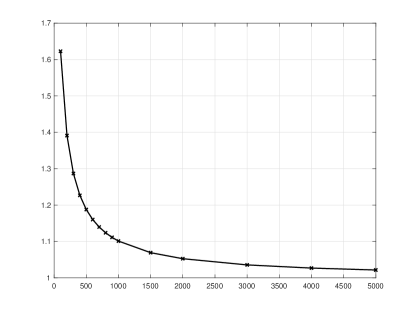
Figure 1: The partial sum of the correlation coefficients in (44) with $\ell_{1}=3N/4$ as a function of $N$. The crosses represent the values of the partial sum that have been computed.

VI Extension to Multidimensional Random Fields

We want to point out that the results obtained in Secs. IV and V transit smoothly to the multidimensional case. In order to see this, let $y_{\mathbf{t}}$ be a zero-mean stationary $d$-dimensional complex-valued random field where $\mathbf{t}=(t_{1},\dots,t_{d})\in\mathbb{Z}^{d}$. Given a vector $\mathbf{N}=(N_{1},\dots,N_{d})\in\mathbb{N}_{+}^{d}$, define a finite index set

$$\mathbb{Z}^{d}_{\mathbf{N}}:=\left\{(t_{1},\dots,t_{d})\,:\,0\leq t_{j}\leq N_{j}-1,\ j=1,\dots,d\right\},$$ (47)

which is just the integer grid of a $d$-dimensional box with a cardinality $|\mathbf{N}|:=\prod_{j=1}^{d}N_{j}$. Suppose that we have obtained samples of the field $\{y_{\mathbf{t}}:\mathbf{t}\in\mathbb{Z}^{d}_{\mathbf{N}}\}$. The spectral domain now becomes $\mathbb{T}^{d}$ containing frequency vectors $\boldsymbol{\theta}=(\theta_{1},\dots,\theta_{d})$. For the computation of the DFT, the multidimensional counterpart of (11) for the discretization of $\mathbb{T}^{d}$ is given as

$$\mathbb{T}^{d}_{\mathbf{N}}:=\left\{\left(\frac{2\pi}{N_{1}}\ell_{1},\dots,\frac{2\pi}{N_{d}}\ell_{d}\right)\in\mathbb{T}^{d}:\boldsymbol{\ell}\in\mathbb{Z}_{\mathbf{N}}^{d}\right\}.$$ (48)

Obviously, the map $\boldsymbol{\ell}\mapsto\boldsymbol{\theta}_{\boldsymbol{\ell}}:=({2\pi\ell_{1}}/{N_{1}},\dots,{2\pi\ell_{d}}/{N_{d}})$ is a bijection from $\mathbb{Z}_{\mathbf{N}}^{d}$ to $\mathbb{T}_{\mathbf{N}}^{d}$. The spectral components are given by the multidimensional DFT

$$Y_{\boldsymbol{\ell}}:=Y(\boldsymbol{\theta}_{\boldsymbol{\ell}})=\sum_{t\in\mathbb{Z}_{\mathbf{N}}^{d}}y_{\mathbf{t}}\,e^{-i\langle{\mathbf{t}},\,{\boldsymbol{\theta}_{\boldsymbol{\ell}}}\rangle},\quad\boldsymbol{\theta}_{\boldsymbol{\ell}}\in\mathbb{T}_{\mathbf{N}}^{d}$$ (49)

whose normalized version is $\bar{Y}_{\boldsymbol{\ell}}:=\frac{1}{\sqrt{|\mathbf{N}|}}Y_{\boldsymbol{\ell}}$. The periodogram is still given by $\hat{\Phi}_{\boldsymbol{\ell}}=|\bar{Y}_{\boldsymbol{\ell}}|^{2}$. The multidimensional version of Theorem 1 is summarized below.

Proposition 2.

Assume that the normalized spectral components $\{\bar{Y}_{\boldsymbol{\ell}}:\boldsymbol{\ell}\in\mathbb{Z}_{\mathbf{N}}^{d}\}$ of the random field $\{y_{\mathbf{t}}:\mathbf{t}\in\mathbb{Z}_{\mathbf{N}}^{d}\}$ are independent zero-mean complex (circular) Gaussian random variables such that $\mathop{\rm var}\bar{Y}_{\boldsymbol{\ell}}={\mathbb{E}}\,\hat{\Phi}_{\boldsymbol{\ell}}=\lambda_{\boldsymbol{\ell}}>0$. Assume in addition that the underlying true spectral density $\Phi(\boldsymbol{\theta})$ of the field $y_{\mathbf{t}}$ satisfies some regularity properties as discussed in Remarks 2 and 3. Then, the estimator

$$\hat{m}_{\mathbf{k}}=\begin{cases}\frac{1}{\alpha|\mathbf{N}|}\sum_{\boldsymbol{\ell}\in\mathbb{Z}_{\mathbf{N}}^{d}}e^{i\langle{\mathbf{k}},\,{\boldsymbol{\theta}_{\boldsymbol{\ell}}}\rangle}\hat{\Phi}_{\boldsymbol{\ell}}^{\alpha}&\text{if }\mathbf{k}\neq\boldsymbol{0},\\ \\ \frac{1}{\alpha}\left(\frac{1}{|\mathbf{N}|}\sum_{\boldsymbol{\ell}\in\mathbb{Z}_{\mathbf{N}}^{d}}\hat{\Phi}_{\boldsymbol{\ell}}^{\alpha}-1\right)&\text{if }\mathbf{k}=\boldsymbol{0}\end{cases}$$ (50)

of the generalized cepstral coefficients

$$m_{\mathbf{k}}=\begin{cases}\frac{1}{\alpha}\int_{\mathbb{T}^{d}}e^{i\langle{\mathbf{k}},\,{\boldsymbol{\theta}}\rangle}\Phi(\boldsymbol{\theta})^{\alpha}\mathrm{d}\mu(\boldsymbol{\theta})&\text{if }\mathbf{k}\neq\boldsymbol{0},\\ \\ \frac{1}{\alpha}\left[\int_{\mathbb{T}^{d}}\Phi(\boldsymbol{\theta})^{\alpha}\mathrm{d}\mu(\boldsymbol{\theta})-1\right]&\text{if }\mathbf{k}=\boldsymbol{0}\end{cases}$$ (51)

is consistent up to a constant multiplicative factor. Here $\mathrm{d}\mu(\boldsymbol{\theta})=\frac{1}{(2\pi)^{d}}\prod_{j=1}^{d}\mathrm{d}\theta_{j}$ is the normalized Lebesgue measure on $\mathbb{T}^{d}$. More precisely, we have for $\mathbf{k}\neq\boldsymbol{0}$ the convergence

$$C\hat{m}_{\mathbf{k}}\xrightarrow{\text{m.s.}}m_{\mathbf{k}},\ \text{ and }\ C\hat{m}_{\boldsymbol{0}}+{(C-1)}/{\alpha}\xrightarrow{\text{m.s.}}m_{\boldsymbol{0}}$$ (52)

as $\min(\mathbf{N})\to\infty$, where the constant $C=1/\Gamma(\alpha+1)$.

Notice that the proof of the above proposition is almost identical to that in the unidimensional case (hence omitted), as the computation of the quantities such as (25) and (29) is left unchanged. The only difference in the multidimensional case is that we need to use multiple indices for the summation and write multivariable integrals. For example, (33) should be rewritten as

$$\frac{1}{|\mathbf{N}|}\sum_{\boldsymbol{\ell}\in\mathbb{Z}_{\mathbf{N}}^{d}}\lambda_{\boldsymbol{\ell}}^{2\alpha}\to\int_{\mathbb{T}^{d}}\Phi(\boldsymbol{\theta})^{2\alpha}\mathrm{d}\mu(\boldsymbol{\theta}).$$ (53)

As for the case with correlated spectral components, we can either use windowing techniques as explained in [18, Sec. 9.7] for the 2-d case and in [33, 34] for 3-d radar signal processing, or make an argument along the lines of Section V where conditions in Assumption 2 are now replaced by

$$\lim_{\min(\mathbf{N})\to\infty}\gamma_{\mathbf{N}}<\infty,\quad\sum_{\boldsymbol{\ell}_{2}\in\mathbb{Z}_{\mathbf{N}}^{d}}\rho_{\boldsymbol{\ell}_{1}\boldsymbol{\ell}_{2}}^{2}\leq f(\mathbf{N}),\quad\forall\boldsymbol{\ell}_{1}\in\mathbb{Z}_{\mathbf{N}}^{d},$$

where

$$\gamma_{\mathbf{N}}:=\max_{\boldsymbol{\ell}\in\mathbb{Z}_{\mathbf{N}}^{d}}\,\lambda_{\boldsymbol{\ell}},\quad\lim_{\min(\mathbf{N})\to\infty}f(\mathbf{N})/|\mathbf{N}|=0.$$

VII Cascade System Identification

In this section, we show that our generalized cepstral estimator can be integrated into a spectral estimation procedure for the identification of cascade (possibly multidimensional) linear stochastic systems with identical subsystems, see Fig. 2 where $W(z)$ denotes the transfer function of each subsystem, $y_{t}$ is the output, and $e_{t}$ is the white noise input. In practice, of course the system need not be driven by a white noise but rather has an input $u_{t}$ which can be modeled as a stationary stochastic process. The output of the cascade system then becomes (symbolically) $y_{t}=[W(z)]^{2}u_{t}$. Assume that we are able to measure both $y_{t}$ and $u_{t}$. At that point one can estimate the power spectral density of the input and thus also its shaping filter $\hat{W}_{u}$. After that, we can filter the output to obtain $\tilde{y}_{t}=[\hat{W}_{u}(z)]^{-1}y_{t}$ which approximately admits the model of Fig. 2. In this sense we have whitened the input process. Therefore, it is not restrictive to consider a white noise input in the cascade system above.

A cascade of identical systems is commonly used to model reactors in chemical engineering: each subsystem corresponds to a continuous stirred-tank reactor (CSTR) and the aim of the cascade is to increase the residence time distribution (RTD) of the reactor [35]. Moreover, the multidimensional setting allows to model the fact that influent and effluent concentration distributions are non-uniform, see for instance [36].

We assume that the number of subsystems which we call $\nu$, is a priori known so that the parameter $\alpha$ is specialized as $1-\frac{1}{\nu}$ (see also Example 1 in Section IV). The latter choice of the parameter turns out to correctly recover the number of subsystems. At the heart of our system identification approach lies a spectral estimation problem presented in [16, 20] which we shall briefly recall next.

Figure 2: A cascade linear stochastic system with two identical subsystems.

Suppose that from some underlying random field we are given a number of covariances $\{c_{\mathbf{k}}:\mathbf{k}\in\Lambda\}$ and generalized cepstral coefficients $\{m_{\mathbf{k}}:\mathbf{k}\in\Lambda_{0}\}$, and from these numbers we want to reconstruct the spectrum $\Phi(\boldsymbol{\theta})$, a nonnegative function in $L^{1}(\mathbb{T}^{d})$. Here the index set $\Lambda$ can be any finite set that contains the zero vector and is symmetric with respect to the origin, namely $\mathbf{k}\in\Lambda\implies-\mathbf{k}\in\Lambda$. The other index set $\Lambda_{0}:=\Lambda\backslash\{\boldsymbol{0}\}$ so $m_{\boldsymbol{0}}$ is excluded for technical reasons. Inspired by the famous Maximum Entropy method [37], we set up the following general optimization problem:

$$\underset{\Phi\geq 0}{\max} \mathbb{H}_{\nu}(\Phi):=\frac{\nu^{2}}{\nu-1}\left(\int_{\mathbb{T}^{d}}\Phi(\boldsymbol{\theta})^{\frac{\nu-1}{\nu}}\mathrm{d}\mu(\boldsymbol{\theta})-1\right)$$ (54a)

s.t. $$c_{\mathbf{k}}=\int_{\mathbb{T}^{d}}e^{i\langle{\mathbf{k}},\,{\boldsymbol{\theta}}\rangle}\Phi(\boldsymbol{\theta})\mathrm{d}\mu(\boldsymbol{\theta})\;\ \forall\mathbf{k}\in\Lambda,$$ (54b)

$$m_{\mathbf{k}}=\frac{\nu}{\nu-1}\int_{\mathbb{T}^{d}}e^{i\langle{\mathbf{k}},\,{\boldsymbol{\theta}}\rangle}\Phi(\boldsymbol{\theta})^{\frac{\nu-1}{\nu}}\mathrm{d}\mu(\boldsymbol{\theta})\;\ \forall\mathbf{k}\in\Lambda_{0},$$ (54c)

where the objective functional $\mathbb{H}_{\nu}(\Phi)$ is a generalized version of the entropy of $\Phi$ derived from the $\alpha$-divergence [38, 39]. The above formulation can be viewed as a considerable generalization of the simultaneous covariance-cepstral extension theory in [15, 40] as their problem can be recovered from ours by letting $\nu\to 1$. The optimization problem in (54) is infinite-dimensional, and it is usually more convenient to work with its finite-dimensional dual problem. Following the analysis in [16], a suitable form of regularization is needed in order to promote a unique positive solution to the dual problem, so that the resulting primal solution $\Phi$ is a strictly positive spectral density which is desired in many practical applications. More specifically, the regularized dual optimization problem is formulated as:

$$\underset{\mathbf{p},\,\mathbf{q}}{\min\,}\ J_{\nu,\lambda}(\mathbf{p},\mathbf{q}):=J_{\nu}(\mathbf{p},\mathbf{q})+\frac{\lambda}{\nu-1}\int_{\mathbb{T}^{d}}\frac{1}{P(\boldsymbol{\theta})^{\nu-1}}\mathrm{d}\mu(\boldsymbol{\theta})$$

$$\hbox{ s.t. }P(\boldsymbol{\theta})\geq 0,\quad Q(\boldsymbol{\theta})\geq 0,\quad\forall\boldsymbol{\theta}\in\mathbb{T}^{d}$$ (55)

where, the dual variables (the Lagrange multipliers) $\{q_{\mathbf{k}}:\mathbf{k}\in\Lambda\}$ and $\{p_{\mathbf{k}}:\mathbf{k}\in\Lambda_{0}\}$ correspond to the covariance and cepstral constraints (54b) and (54c), respectively, $P(\boldsymbol{\theta}):=1+\sum_{\mathbf{k}\in\Lambda_{0}}p_{\mathbf{k}}e^{-i\langle{\mathbf{k}},\,{\boldsymbol{\theta}}\rangle}$ and $Q(\boldsymbol{\theta}):=\sum_{\mathbf{k}\in\Lambda}q_{\mathbf{k}}e^{-i\langle{\mathbf{k}},\,{\boldsymbol{\theta}}\rangle}$ are trigonometric polynomials, and $\lambda>0$ is the regularization parameter. The first term in the dual objective function $J_{\nu,\lambda}(\mathbf{p},\mathbf{q})$ is the unregularized dual function

$$J_{\nu}(\mathbf{p},\mathbf{q}):=\frac{1}{\nu-1}\int_{\mathbb{T}^{d}}\frac{P(\boldsymbol{\theta})^{\nu}}{Q(\boldsymbol{\theta})^{\nu-1}}\mathrm{d}\mu(\boldsymbol{\theta})+\langle\mathbf{q},\mathbf{c}\rangle-\langle\mathbf{p},\mathbf{m}\rangle,$$ (56)

where the real-valued inner product $\langle\mathbf{q},\mathbf{c}\rangle:=\sum_{\mathbf{k}\in\Lambda}q_{\mathbf{k}}c_{\mathbf{k}}^{*}$.

Under a suitable feasibility assumption for the covariance (multi)sequence $\{c_{\mathbf{k}}:\mathbf{k}\in\Lambda\}$ (see [16, Assumption 5.1]), if the integer parameter $\nu$, the number of subsystems in the cascade, satisfies the condition $\nu\geq\frac{d}{2}+1$, then the regularized dual problem (VII) admits a unique solution $(\hat{\mathbf{p}},\hat{\mathbf{q}})$ such that the corresponding polynomials $\hat{P}$ and $\hat{Q}$ are both strictly positive. Moreover, the positive rational function

$$\hat{\Phi}_{\nu}(\boldsymbol{\theta})=[\hat{P}(\boldsymbol{\theta})/\hat{Q}(\boldsymbol{\theta})]^{\nu}$$ (57)

matches the given covariances $\{c_{\mathbf{k}}:\mathbf{k}\in\Lambda\}$ exactly and the generalized cepstral coefficients $\{m_{\mathbf{k}}:\mathbf{k}\in\Lambda_{0}\}$ approximately. Clearly we have set $p_{\boldsymbol{0}}=1$ in order to avoid trivial cancellations between $P$ and $Q$ in the rational function $\Phi_{\nu}$.

From the perspective of numerical computation, it is better to discretize the problems (VII) on a grid similar to (48) but of a different size $\mathbf{K}=(K_{1},\dots,K_{d})\in\mathbb{N}_{+}^{d}$. The formulas will be similar to the ones above and are omitted here. For details see [16, Section 8] where it is also explained that the solution to the discrete problem is a reasonable approximation of the solution to the corresponding continuous problem when the grid size $\mathbf{K}$ is sufficiently large (componentwise).

To summarize, our system identification procedure can be divided into four steps:

(i) Feed the system with normalized white noise $e_{\mathbf{t}}$ and collect the output random field $\{y_{\mathbf{t}}:\mathbf{t}\in\mathbb{Z}_{\mathbf{N}}^{d}\}$;
(ii) Choose an index set $\Lambda$ and estimate $\{c_{\mathbf{k}}:\mathbf{k}\in\Lambda\}$ via (12) adapted to multidimensional random fields (see e.g., [41]) and $\{m_{\mathbf{k}}:\mathbf{k}\in\Lambda_{0}\}$ via (50) corrected with the constant $C$ in (52);
(iii) Fix a grid size $\mathbf{K}$ and solve the discrete version of the regularized dual optimization problem (VII) given $c_{\mathbf{k}}$’s and $m_{\mathbf{k}}$’s in Step (ii) and a regularization parameter $\lambda>0$;
(iv) Factor the optimal spectrum $\hat{\Phi}(\boldsymbol{\theta})$ in order to obtain a transfer function $\hat{W}(\mathbf{z})$ where $\mathbf{z}:=(z_{1},\dots,z_{d})$.

We must point out that there is a significant technical difficulty in the last step of the procedure concerning spectral factorization. Since our optimal spectrum is a rational function, we end up factoring positive Laurent trigonometric polynomials of several variables into one square, which is in general an impossible task. Fortunately in the $2$-d case, [43, Theorems 1.1.1 & 1.1.3] have given a sufficient and necessary condition to check such factorability and an explicit formula to compute the factor when the factorization is possible. The nontrivial part of the condition states that a certain submatrix of the full covariance matrix should have a specific low rank.

In addition, we want to stress that the regularization employed in (VII) has the power of promoting strict convexity and well-posedness of the dual problem [16]. Of course, the regularization term does not appear naturally in the system identification problem. Thus in order to get a reasonable consistency result for the identified model, we should take the regularization parameter $\lambda$ small as it directly controls the error in generalized cepstral matching. The next proposition expresses the idea.

Proposition 3.

Assume that the model class is correctly specified, i.e., the unknown system transfer function $W(\mathbf{z})$ is such that true spectrum of the output random field $y_{\mathbf{t}}$ $($when the input $e_{\mathbf{t}}$ is a normalized white noise$)$ falls within the class of rational functions having the form (57). Then as the number of samples $\min(\mathbf{N})\to\infty$ and the regularization parameter $\lambda\to 0$, the optimal solution to (VII) recovers the true spectrum of $y_{\mathbf{t}}$ as well as the correct system parameters in $W(\mathbf{z})$ after spectral factorization.

Proof.

The proposition is a direct consequence of Theorem 6.1 in [16]. ∎

In plain words the above result says: given a $d$-dimensional system, which is a cascade of $\nu\geq d/2+1$ identical subsystems, it is possible to construct a consistent estimator of it using some second-order statistics of the output process.

VIII Simulation Results

In this section, we present simulation results in $1$-d and $2$-d cascade system identification because theoretical results and algorithms for polynomial spectral factorization are available only when the dimension is such that $d\leq 2$, as highlighted in the previous section.

VIII-A Identification of $1$-D dynamical systems

Consider a $1$-d linear time-invariant (LTI) system described by the transfer function $W(z)$. Furthermore, let $W$ have the cascade structure that corresponds to our optimal spectrum (57), namely $W(z)=\left[W_{1}(z)\right]^{\nu}$ where each subsystem

$$W_{1}(z)=\frac{b(z)}{a(z)}=\frac{\sum_{k=0}^{n}b_{k}z^{-k}}{\sum_{k=0}^{n}a_{k}z^{-k}}.$$ (58)

Here the index set is $\Lambda_{+}=\{0,1,\dots,n\}$ and we take $n=2$ which corresponds to a second-order system for simplicity.

Let us write $a(\theta)\equiv a(e^{i\theta})$ for the value of the polynomial $a(z)$ on the unit circle. If the white noise input $e_{t}$ has unit variance, then the spectral density of the output process $y_{t}$ is $\Phi(\theta)=[P(\theta)/Q(\theta)]^{\nu}$ where $P(\theta)=|b(\theta)|^{2}$, $Q(\theta)=|a(\theta)|^{2}$. We shall take the integer $\nu=3$ which is known by our identification procedure. Moreover, we shall parametrize the polynomials in terms of their roots, that is, $a(z)=(1-r_{a,1}z^{-1})(1-r_{a,2}z^{-1})$ and $b(z)=b_{0}(1-r_{b,1}z^{-1})(1-r_{b,2}z^{-1})$ with $b_{0}$ a normalization constant such that $P(z)=b(z)b(z^{-1})$ has $p_{0}=1$. The true system parameters are specified as $r_{a,1},r_{a,2}=0.5e^{\pm i\pi/3}$ (complex conjugate roots) and $r_{b,1},r_{b,2}=-0.8$ and $0.6$ (real roots), so the system $W_{1}$ (also $W$) has real parameters and is clearly stable and minimum-phase. This in turn gives

$$\mathbf{a} =\begin{bmatrix}a_{0}&a_{1}&a_{2}\end{bmatrix}=\begin{bmatrix}1&-0.5&0.25\end{bmatrix}\ \text{ and }\$$ (59)

$$\mathbf{b} =\begin{bmatrix}b_{0}&b_{1}&b_{2}\end{bmatrix}=\begin{bmatrix}0.8872&0.1774&-0.4259\end{bmatrix}.$$

Next, we follow the system identification procedure listed in the previous section, and demonstrate how to estimate the system parameters $\mathbf{a}$ and $\mathbf{b}$ from the samples of the output process $y_{t}$. Such samples of size $N$ are generated by feeding the normalized real white noise $e_{t}$ to the true system (so $y_{t}$ is also real). Then the covariances and generalized cepstral coefficients of the output $y_{t}$ with the indices in the set $\Lambda=\{k\in\mathbb{Z}\,:\,-2\leq k\leq 2\}$ are estimated using (12) and (17). Due to the symmetry, we only need to compute

$$\hat{\mathbf{c}}=\begin{bmatrix}\hat{c}_{0}&\hat{c}_{1}&\hat{c}_{2}\end{bmatrix}\ \text{ and }\ \hat{\mathbf{m}}=\begin{bmatrix}\hat{m}_{1}&\hat{m}_{2}\end{bmatrix}.$$

In particular, the constant $C$ in Theorem 1 for correcting the generalized cepstral estimation is equal to $1/\Gamma(\frac{5}{3})\approx 1.1077$ with $\alpha=\frac{\nu-1}{\nu}=2/3$. The estimation error is defined as $\|[\hat{\mathbf{c}},\hat{\mathbf{m}}]-[\mathbf{c},\mathbf{m}]\|$ where the true $\mathbf{c}$ and $\mathbf{m}$ are evaluated using the true spectrum. Such errors against different sample sizes $N$ are shown in the orange line of Fig. 3(a) in the double-logarithmic scale (base $10$). At the same time, the yellow line indicates the errors when $\hat{\mathbf{m}}$ is not corrected by the constant $C$. To be more clear, one time series $y_{t}$ of length $N_{\max}=10^{4}$ is generated first and simulations are carried out using the same series truncated to different lengths $N$. One can see the general trend of the orange line that the error reduces as the sample size grows. The unique exception at $N=500$ can be explained as random fluctuation before the convergence of the estimators. In this particular example, the uncorrected generalized cepstral estimator begins to produce a large error (relative to that of the corrected version) after $N=2500$. Such an erratic behavior will be more apparent in the $2$-d example presented in the next subsection.

Then the regularized dual problem (VII) is solved on a discrete grid of size $K=N$ with the estimated $\hat{\mathbf{c}}$, $\hat{\mathbf{m}}$, and $\lambda=10^{-6}$ using a gradient descent algorithm. The algorithm is initialized at $q_{0}=1$ and the rest variables equal to $0$ which corresponds to constant polynomials $P(\theta)=Q(\theta)\equiv 1$. The iterations terminate when the norm of the gradient is less than $10^{-6}$. Given the optimal polynomials $\hat{P}$ and $\hat{Q}$, we proceed to compute their factors $\hat{a}$ and $\hat{b}$ using standard methods for ($1$-d) polynomial spectral factorization, e.g., the Bauer method [44]. After a comparison with (59), we compute the error $\|[\hat{\mathbf{a}},\hat{\mathbf{b}}]-[\mathbf{a},\mathbf{b}]\|$ which is shown in the blue line of Fig. 3(a) for different values of $N$. The blue line shares the same trend with the orange line as the sample size $N$ increases, which is an expected result since the true system $W(z)$ belongs to the model class dictated by the solution form (57) of our optimization problem, as explained in Proposition 3. Furthermore, in Fig. 3(b) we plot the true spectrum $\Phi(\theta)$ on the interval $[0,\pi)$ against the estimated spectra $\hat{\Phi}(\theta)$. The convergence of the estimated spectra to the true one is clearly observed.

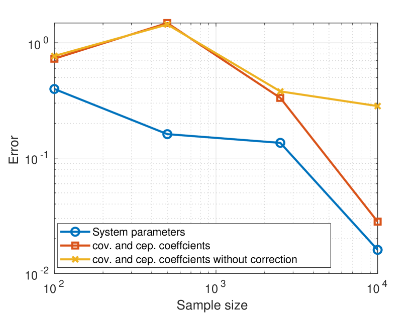
(a)

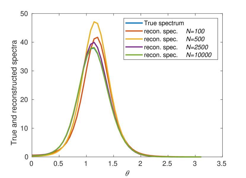
(b)

Figure 3: Simulation results in the $1$-d case: Left. Estimation errors of the covariances and the generalized cepstral coefficients (the orange line with correction and the yellow line without correction) and the system parameters (blue line) when the sample size $N$ of the random process is equal to $100,500,2500,10^{4}$. Right. The true spectrum (blue line) $\Phi(\theta)$ of $y_{t}$ versus the estimated spectra $\hat{\Phi}(\theta)$ via solving the discrete version of the regularized dual optimization problem (VII) with $\lambda=10^{-6}$ and the sample sizes indicated above. Only the segment corresponding to $\theta\in[0,\pi)$ is shown due to the symmetry of the spectra of real processes. Notice that the estimated spectrum with $N=10^{4}$ virtually coincide with the true one.

VIII-B Modeling $2$-D random fields

In this subsection, we consider the problem of identifying a $2$-d LTI system $W(z_{1},z_{2})$ from samples of a planar random process. The procedure will be similar to the previous subsection which we will describe briefly. Let $W(\mathbf{z})=\left[W_{1}(\mathbf{z})\right]^{\nu}$ with $\nu=2$ and the subsystem

$$W_{1}(\mathbf{z})=\frac{b(\mathbf{z})}{a(\mathbf{z})}=\frac{\sum_{\mathbf{k}\in\Lambda_{+}}b_{\mathbf{k}}\mathbf{z}^{-\mathbf{k}}}{\sum_{\mathbf{k}\in\Lambda_{+}}a_{\mathbf{k}}\mathbf{z}^{-\mathbf{k}}},$$ (60)

where the index set $\Lambda_{+}:=\{(k_{1},k_{2})\in\mathbb{Z}^{2}\,:\,0\leq k_{1},k_{2}\leq 1\}$ so that $W_{1}$ (roughly) has order one in each dimension, the indeterminates $(z_{1},z_{2})$ are abbreviated as $\mathbf{z}$, and $\mathbf{z}^{\mathbf{k}}$ stands for $z_{1}^{k_{1}}z_{2}^{k_{2}}$. For notational convenience, the value of the polynomial $a(\mathbf{z})$ on the unit torus is written as $a(\boldsymbol{\theta})\equiv a(e^{i\theta_{1}},e^{i\theta_{2}})$. For simplicity, we also impose a separable form $(1-r_{a,1}z_{1}^{-1})(1-r_{a,2}z_{2}^{-1})$ on the polynomials $a$, $b$, and take $|r_{a,j}|<1$ for $j=1,2$. The system parameters can be assigned via

$$\begin{bmatrix}a_{0,0}&a_{0,1}&a_{1,0}&a_{1,1}\end{bmatrix}=\begin{bmatrix}1&-r_{a,2}&-r_{a,1}&r_{a,1}r_{a,2}\end{bmatrix}.$$

It is convenient to collect the $2$-d system parameters into matrices. In our particular example, we take real parameters

$$A=\begin{bmatrix}1&-0.7\\ -0.5&0.35\end{bmatrix},\quad B=\begin{bmatrix}0.6696&-0.5357\\ -0.4018&0.3214\end{bmatrix}$$ (61)

where $a_{k_{1},k_{2}}=A(k_{1}+1,k_{2}+1)$ and similar for $b_{k_{1},k_{2}}$. Notice that the constraint $p_{\boldsymbol{0}}=1$ translates into a normalization condition $\|B\|_{\mathrm{F}}=1$ where the subscript _F denotes the Frobenius norm. The true spectrum $\Phi(\boldsymbol{\theta})$ defined on the $2$-d domain is shown in Fig. 4(b).

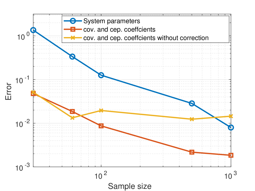
(a)

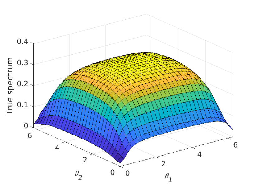
(b)

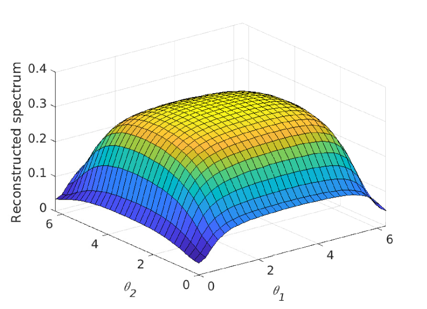
(c)

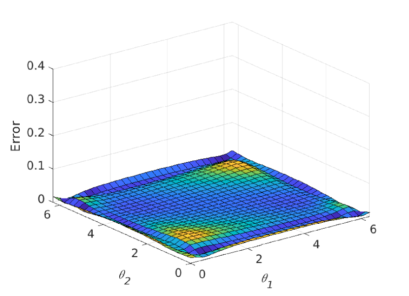
(d)

Figure 4: Simulation results in the $2$-d case: Upper left. Estimation errors of the covariances and the generalized cepstral coefficients (the orange line with correction and the yellow line without correction) and the system parameters (blue line) when the sample size $N_{1}=N_{2}=N$ of the random field is equal to $30,60,100,500,1000$. Upper right. The true spectrum $\Phi(\boldsymbol{\theta})$ of $y_{\mathbf{t}}$. Lower left. The estimated spectrum $\hat{\Phi}(\boldsymbol{\theta})$ via solving the discrete version of the regularized dual optimization problem (VII) with $\lambda=10^{-6}$ and the sample size $N=100$. Lower right. The pointwise absolute error $|\hat{\Phi}(\boldsymbol{\theta})-\Phi(\boldsymbol{\theta})|$ between Subfigs. 4(b) and 4(c).

Next we implement the system identification procedure in order to estimate the “system matrices” $A$ and $B$ from the samples of the output process $y_{\mathbf{t}}$ with a size $\mathbf{N}=(N_{1},N_{2})$. The covariances and generalized cepstral coefficients of $y_{\mathbf{t}}$ indexed by the set $\Lambda=\{(k_{1},k_{2})\in\mathbb{Z}^{2}\,:\,-1\leq k_{1},k_{2}\leq 1\}$ are estimated using the unwindowed periodogram as explained in Section VI. Due to the symmetry of $c_{\mathbf{k}}$ and $m_{\mathbf{k}}$ with respect to the origin, we only need to compute

$$\hat{\mathbf{c}} =\begin{bmatrix}\hat{c}_{0,0}&\hat{c}_{0,1}&\hat{c}_{1,-1}&\hat{c}_{1,0}&\hat{c}_{1,1}\end{bmatrix},$$

$$\hat{\mathbf{m}} =\begin{bmatrix}\hat{m}_{0,1}&\hat{m}_{1,-1}&\hat{m}_{1,0}&\hat{m}_{1,1}\end{bmatrix}$$

which are put in the lexicographic ordering. In particular, the constant of correction $C$ in (52) is now $1/\Gamma(\frac{3}{2})=2/\sqrt{\pi}\approx 1.1284$ since $\alpha=1-\frac{1}{\nu}=1/2$. The estimation error $\|[\hat{\mathbf{c}},\hat{\mathbf{m}}]-[\mathbf{c},\mathbf{m}]\|$ versus the sample size $N_{1}=N_{2}=N$ is plotted in the orange line of Fig. 4(a) which shares the same trend as that in Fig. 3(a): the error goes down as the sample size increases. The yellow line corresponding to the wrong generalized cepstral estimator, in contrast, deviates from the orange line as early as $N=100$ in this example. Obviously, the wrong estimator does not enjoy the consistency property since the error curve stops going down as $N$ further increases.

Then we solve the regularized dual problem (VII) on a discrete grid of fixed size $\mathbf{K}=(30,30)$ with the estimated $\hat{\mathbf{c}}$, $\hat{\mathbf{m}}$, and $\lambda=10^{-6}$. The optimal spectrum $\hat{\Phi}(\boldsymbol{\theta})$ returned by the solver is shown in Fig. 4(c) when the sample size is $N_{1}=N_{2}=100$. In this case, clearly the shape of the estimated spectrum is almost visually indistinguishable from that of the true spectrum. Moreover, the pointwise absolute error $|\hat{\Phi}(\boldsymbol{\theta})-\Phi(\boldsymbol{\theta})|$ is shown in Fig. 4(d). One can see that the error plot is quite flat. As a complement, we also compute the cumulative relative error on the whole grid $\|\hat{\Phi}-\Phi\|_{\mathrm{F}}/\|\Phi\|_{\mathrm{F}}=4.40\%$ which is reasonably small.

Once we have the optimal polynomials $\hat{P}$ and $\hat{Q}$, we can run the factorization algorithm in [43, Theorems 1.1.1 & 1.1.3] and compute factors $\hat{a}$ and $\hat{b}$. The numerical values of their coefficients in this particular instance with a sample size $N=100$ are reported in the following matrices

$$\hat{A}=\begin{bmatrix}1.0590&-0.6896\\ -0.4503&0.2854\end{bmatrix},\quad\hat{B}=\begin{bmatrix}0.7102&-0.5282\\ -0.3679&0.2688\end{bmatrix}.$$

The error here is $\|[\hat{A},\hat{B}]-[A,B]\|_{\mathrm{F}}=0.1259$ which, along with other errors for different $N$, is depicted in the blue line of Fig. 4(a). We can see the consistency of our identification procedure as reported in Proposition 3.

IX Conclusions

We have proposed an estimator for the generalized cepstral coefficients both in the unidimensional and multidimensional setting. We showed that it is consistent in the special case that the stochastic process is i.i.d. or periodic. We also provided a condition that guarantees the consistency in the general case where the spectral components are correlated. Such a condition seems to be satisfied when the stochastic process is generated by a stable rational filter. Finally, we showed that this estimator can be used to build a consistent estimator for a class of cascade linear stochastic systems.

References

- [1] C. I. Byrnes, S. V. Gusev, and A. Lindquist, “A convex optimization approach to the rational covariance extension problem,” SIAM Journal on Control Optimization, vol. 37, no. 1, pp. 211–229, 1998.
- [2] ——, “From finite covariance windows to modeling filters: A convex optimization approach,” SIAM Review, vol. 43, no. 4, pp. 645–675, 2001.
- [3] T. T. Georgiou, “Spectral estimation via selective harmonic amplification,” IEEE Transactions on Automatic Control, vol. 46, no. 1, pp. 29–42, 2001.
- [4] C. Byrnes, P. Enqvist, and A. Lindquist, “Cepstral coefficients, covariance lags, and pole-zero models for finite data strings,” IEEE Transactions on Signal Processing, vol. 49, no. 4, pp. 677–693, 2001.
- [5] A. Ferrante, M. Pavon, and F. Ramponi, “Hellinger versus Kullback–Leibler multivariable spectrum approximation,” IEEE Transactions on Automatic Control, vol. 53, no. 4, pp. 954–967, 2008.
- [6] A. Ferrante, F. Ramponi, and F. Ticozzi, “On the convergence of an efficient algorithm for Kullback–Leibler approximation of spectral densities,” IEEE Transactions on Automatic Control, vol. 56, no. 3, pp. 506–515, 2011.
- [7] F. Ramponi, A. Ferrante, and M. Pavon, “A globally convergent matricial algorithm for multivariate spectral estimation,” IEEE Transactions on Automatic Control, vol. 54, no. 10, pp. 2376–2388, 2009.
- [8] A. Ringh, J. Karlsson, and A. Lindquist, “Multidimensional rational covariance extension with approximate covariance matching,” SIAM Journal on Control and Optimization, vol. 56, no. 2, pp. 913–944, 2018.
- [9] B. Zhu, “On the well-posedness of a parametric spectral estimation problem and its numerical solution,” IEEE Transactions on Automatic Control, vol. 65, no. 3, pp. 1089–1099, 2020.
- [10] A. Ferrante, C. Masiero, and M. Pavon, “Time and spectral domain relative entropy: A new approach to multivariate spectral estimation,” IEEE Transactions on Automatic Control, vol. 57, no. 10, pp. 2561–2575, 2012.
- [11] M. Zorzi, “A new family of high-resolution multivariate spectral estimators,” IEEE Transactions on Automatic Control, vol. 59, no. 4, pp. 892–904, 2014.
- [12] B. Zhu and G. Baggio, “On the existence of a solution to a spectral estimation problem à la Byrnes-Georgiou-Lindquist,” IEEE Transactions on Automatic Control, vol. 64, no. 2, pp. 820–825, 2019.
- [13] Y. Ephraim and M. Rahim, “On second-order statistics and linear estimation of cepstral coefficients,” IEEE Transactions on Speech and Audio Processing, vol. 7, no. 2, pp. 162–176, 1999.
- [14] Y. Ephraim and W. J. Roberts, “On second-order statistics of log-periodogram with correlated components,” IEEE Signal Processing Letters, vol. 12, no. 9, pp. 625–628, 2005.
- [15] P. Enqvist, “A convex optimization approach to ARMA model design from covariance and cepstral data,” SIAM Journal on Control and Optimization, vol. 43, no. 3, pp. 1011–1036, 2004.
- [16] B. Zhu and M. Zorzi, “Multidimensional rational covariance and cepstral extension: A general formulation,” Submitted to SIAM Journal on Control and Optimization, 2021.
- [17] F. Ramponi, A. Ferrante, and M. Pavon, “On the well-posedness of multivariate spectrum approximation and convergence of high-resolution spectral estimators,” Systems & Control Letters, vol. 59, no. 3, pp. 167–172, 2010.
- [18] M. B. Priestley, Spectral Analysis and Time Series (Two-Volume Set), ser. Probability and Mathematical Statistics. Elsevier Academic Press, 1981, reprinted in 2004.
- [19] J. Karlsson, A. Lindquist, and A. Ringh, “The multidimensional moment problem with complexity constraint,” Integral Equations and Operator Theory, vol. 84, no. 3, pp. 395–418, 2016.
- [20] B. Zhu and M. Zorzi, “A generalized multidimensional circulant rational covariance and cepstral extension problem,” in IFAC PapersOnLine, vol. 54, no. 7. Padova, Italy: IFAC, 2021, pp. 553–558, presented virtually at the 19th IFAC Symposium on System Identification (SYSID 2021).
- [21] A. Ringh, J. Karlsson, and A. Lindquist, “The multidimensional circulant rational covariance extension problem: Solutions and applications in image compression,” in 54th Annual Conference on Decision and Control (CDC). IEEE, 2015, pp. 5320–5327.
- [22] K. Tokuda, T. Kobayashi, and S. Imai, “Generalized cepstral analysis of speech-unified approach to LPC and cepstral method,” in First International Conference on Spoken Language Processing, 1990.
- [23] B. Wahlberg, H. Hjalmarsson, and J. Mårtensson, “Variance results for identification of cascade systems,” Automatica, vol. 45, no. 6, pp. 1443–1448, 2009.
- [24] H. Sandberg, P. Hägg, and B. Wahlberg, “Approximative model reconstruction of cascade systems,” Systems & Control Letters, vol. 69, pp. 90–97, 2014.
- [25] A. Lindquist and G. Picci, Linear Stochastic Systems: A Geometric Approach to Modeling, Estimation and Identification, ser. Series in Contemporary Mathematics. Springer-Verlag Berlin Heidelberg, 2015, vol. 1.
- [26] P. Stoica and R. Moses, Spectral Analysis of Signals. Upper Saddle River, NJ: Pearson Prentice Hall, 2005.
- [27] R. M. Gray, “Toeplitz and circulant matrices: A review,” Foundations and Trends in Communications and Information Theory, vol. 2, no. 3, pp. 155–239, 2006.
- [28] A. Lindquist and G. Picci, “The circulant rational covariance extension problem: The complete solution,” IEEE Transactions on Automatic Control, vol. 58, no. 11, pp. 2848–2861, 2013.
- [29] I. S. Gradshteyn and I. M. Ryzhik, Table of Integrals, Series, and Products, 8th ed. Academic Press, 2014.
- [30] A. Villani, “Another note on the inclusion ,” The American Mathematical Monthly, vol. 92, no. 7, pp. 485–487, 1985.
- [31] M. Abramowitz and I. A. Stegun, Eds., Handbook of Mathematical Functions with Formulas, Graphs, and Mathematical Tables, 10th ed., ser. National Bureau of Standards Applied Mathematics Series. U.S. Government Printing Office, 1972, vol. 55, reprinted by Dover Publications in 2020 with corrections.
- [32] R. B. Davies, “Algorithm AS155: The distribution of a linear combination of random variables,” Applied Statistics, pp. 323–333, 1980.
- [33] F. Engels, P. Heidenreich, A. M. Zoubir, F. K. Jondral, and M. Wintermantel, “Advances in automotive radar: A framework on computationally efficient high-resolution frequency estimation,” IEEE Signal Processing Magazine, vol. 34, no. 2, pp. 36–46, 2017.
- [34] B. Zhu, A. Ferrante, J. Karlsson, and M. Zorzi, “Fusion of sensors data in automotive radar systems: A spectral estimation approach,” in 58th IEEE Conference on Decision and Control (CDC 2019). IEEE, 2019, pp. 5088–5093.
- [35] A. Renken, M. N. Kashid, and L. Kiwi-Minsker, Microstructured Devices for Chemical Processing. John Wiley & Sons, 2014.
- [36] V. Vavilin, L. Lokshina, X. Flotats, and I. Angelidaki, “Anaerobic digestion of solid material: Multidimensional modeling of continuous-flow reactor with non-uniform influent concentration distributions,” Biotechnology and Bioengineering, vol. 97, no. 2, pp. 354–366, 2007.
- [37] J. P. Burg, “Maximum entropy spectral analysis,” Ph.D. dissertation, Department of Geophysics, Stanford University, 1975.
- [38] M. Zorzi, “Rational approximations of spectral densities based on the Alpha divergence,” Mathematics of Control, Signals, and Systems, vol. 26, no. 2, pp. 259–278, 2014.
- [39] ——, “An interpretation of the dual problem of the THREE-like approaches,” Automatica, vol. 62, pp. 87–92, 2015.
- [40] A. Ringh, J. Karlsson, and A. Lindquist, “Multidimensional rational covariance extension with applications to spectral estimation and image compression,” SIAM Journal on Control and Optimization, vol. 54, no. 4, pp. 1950–1982, 2016.
- [41] B. Zhu, A. Ferrante, J. Karlsson, and M. Zorzi, “M2-spectral estimation: A relative entropy approach,” Automatica, vol. 125, March 2021.
- [42] M. A. Dritschel, “On factorization of trigonometric polynomials,” Integral Equations and Operator Theory, vol. 49, no. 1, pp. 11–42, 2004.
- [43] J. S. Geronimo and H. J. Woerdeman, “Positive extensions, Fejér-Riesz factorization and autoregressive filters in two variables,” Annals of Mathematics, vol. 160, no. 3, pp. 839–906, 2004.
- [44] A. H. Sayed and T. Kailath, “A survey of spectral factorization methods,” Numerical Linear Algebra with Applications, vol. 8, no. 6-7, pp. 467–496, 2001.