A nested divide-and-conquer method for tensor Sylvester equations with positive definite hierarchically semiseparable coefficients

Abstract

Linear systems with a tensor product structure arise naturally when considering the discretization of Laplace type differential equations or, more generally, multidimensional operators with separable coefficients. In this work, we focus on the numerical solution of linear systems of the form

$$\left(I\otimes\dots\otimes I\otimes A_{1}+\dots+A_{d}\otimes I\otimes\dots\otimes I\right)x=b,$$

where the matrices $A_{t}\in\mathbb{R}^{n\times n}$ are symmetric positive definite and belong to the class of hierarchically semiseparable matrices.

We propose and analyze a nested divide-and-conquer scheme, based on the technology of low-rank updates, that attains the quasi-optimal computational cost $\mathcal{O}(n^{d}\log(n))$. Our theoretical analysis highlights the role of inexactness in the nested calls of our algorithm and provides worst case estimates for the amplification of the residual norm. The performances are validated on 2D and 3D case studies.

Keywords Tensor equation, Sylvester equation, Divide and conquer, Rational approximation.

Mathematics Subject Classification 15A06, 65F10, 65Y20

1 Introduction

In this work we are concerned with the numerical solution of linear systems with a Kronecker sum-structured coefficient matrix of the form:

$$\left(I\otimes\dots\otimes I\otimes A_{1}+\dots+A_{d}\otimes I\otimes\dots\otimes I\right)x=b,$$ (1)

where the matrices $A_{t}\in\mathbb{R}^{n_{t}\times n_{t}}$ are symmetric and positive definite (SPD) with spectrum contained in $[\alpha_{t},\beta_{t}]\subset\mathbb{R}^{+}:=\{z\in\mathbb{R}\ \text{s.t.}\ z>0\}$, and have low-rank off-diagonal blocks, for $t=1,\dots,d$. By reshaping $x,b\in\mathbb{R}^{n_{1}\dots n_{d}}$ into $d$-dimensional tensors $\mathcal{X},\mathcal{B}\in\mathbb{R}^{n_{1}\times\dots n_{d}}$, we rewrite (1) as the tensor Sylvester equation

$$\mathcal{X}\times_{1}A_{1}+\dots+\mathcal{X}\times_{d}A_{d}=\mathcal{B},$$ (2)

where $\times_{j}$ denotes the $j$-mode product for tensors [kolda, Section 2.6].

Tensor Sylvester equations, not necessarily with SPD coefficients, arise naturally when discretizing $d$-dimensional Laplace-like operators by means of tensorized grids that respect the separability of the operator [townsend2015automatic, townsend-fortunato, strossner2021fast, palitta2016matrix, massei2021rational]. In the case $d=2$, we recover the well-known case of matrix Sylvester equations, that also plays a dominant role in the model reduction of dynamical systems [antoulas-approximation].

Several methods for solving matrix and tensor Sylvester equations assume that the right-hand side has some structure, such as being low-rank. This is a necessary assumption for dealing with large scale problems. In this paper, we only consider unstructured right-hand sides $\mathcal{B}$, for which the cases of interest are those where the memory cost $\mathcal{O}(\prod_{t=1}^{d}n_{t})$ still allows storing $\mathcal{B}$ and the solution $\mathcal{X}$. Note that, this limits the scenarios where our algorithm is effective to small values of $d$, i.e. $d=2,3$. The structure in the coefficients $A_{t}$ (which are SPD and have off-diagonal blocks of low-rank), will be crucial to improve the complexity of the solver with respect to the completely unstructured case. We also remark that when the $A_{t}$s arise from the discretization of elliptic differential operators, the structure assumed in this work is often present [hackbusch, borm].

1.1 Related work

In the matrix case (i.e., $d=2$ in (2)) there are two main procedures that make no assumptions on $A_{1},A_{2},$ and $\mathcal{B}$: the Bartels-Stewart algorithm [bartels-stewart, recursive-sylvester-kagstrom] and the Hessenberg-Schur method [hessenberg-schur]. These are based on taking the coefficients $A_{1},A_{2}$ to either Hessenberg or triangular form, and then solving the linear system by (block) back-substitution. The idea has been generalized to $d$-dimensional tensor Sylvester equations in [chen2020recursive]. In the case where $n=n_{1}=\ldots=n_{d}$, the computational complexity of these approaches is $\mathcal{O}(dn^{3}+n^{d+1})$ flops.

When $d=2$ and the right-hand side $\mathcal{B}$ is a low-rank matrix or $d>2$ and $\mathcal{B}$ is representable in a low-rank tensor format (Tucker, Tensor-Train, Hierarchical Tucker, …) the tensor equation can be solved much more efficiently, and the returned approximate solution is low-rank, which allows us to store it in a low-memory format. Indeed, in this case it is possible to exploit tensorized Krylov (and rational Krylov) methods [Simoncini2016, druskin2011analysis, kressner2009krylov], or the factored Alternating Direction Implicit Method (fADI) [benner2009adi, shi21]. The latter methods build a rank $s$ approximant to the solution $\mathcal{X}$ by solving $\mathcal{O}(s)$ shifted linear systems with the matrices $A_{t}$. This is very effective when also the coefficients $A_{t}$ are structured. For instance, when the $A_{t}$ are sparse or hierarchically low-rank, this often brings the cost of approximating $X$ to $\mathcal{O}(sn\log^{a}n)$ for $a\in\{0,1,2\}$ [hackbusch]. In the tensor case, another option is to rely on methods adapted to the low-rank structure under consideration: AMEn [dolgov2014alternating] or TT-GMRES [dolgov2013tt] for Tensor-Trains, projection methods in the Hierarchical Tucker format [ballani2013projection], and other approaches.

In this work, we consider an intermediate setting, where the coefficients $A_{t}$ are structured, while the right-hand side $\mathcal{B}$ is not. More specifically, we assume that the $A_{t}$ are SPD and efficiently representable in the Hierarchical SemiSeparable format (HSS) [xia2010fast]. This implies that each coefficient $A_{t}$ can be partitioned in a $2\times 2$ block matrix with low-rank off-diagonal blocks, and diagonal blocks with the same recursive structure.

A particular case of this setting has been considered in [townsend-fortunato], where the $A_{t}$ are banded SPD (and therefore have low-rank off-diagonal blocks), and a nested Alternating Direction Implicit (ADI) solver is applied to a 3D tensor equation with no structure in $\mathcal{B}$. The complexity of the algorithm is quasi-optimal $\mathcal{O}(n^{3}\log^{3}n)$, but the hidden constant is very large, and the approach is not practical already for moderate $n$; see [strossner2021fast] for a comparison with methods with a higher asymptotic complexity.

We remark that, when the coefficients $A_{t}$ are SPD, the tensor equation (2) can be solved by diagonalization of the $A_{t}$s in a stable way, as described in the pseudocode of Algorithm 1. Without further assumptions, this costs $\mathcal{O}(dn^{3}+n^{d+1})$ when all dimensions are equal.

Algorithm 1

1:procedure lyapnd_diag($A_{1},A_{2},\dots,A_{d},\mathcal{B}$)

2:    for $i=1,\dots,d$ do

3:         $[S_{i},D_{i}]=\texttt{eig}(A_{i})$

4:         $\mathcal{B}\leftarrow\mathcal{B}\times_{i}S_{i}^{*}$

5:    end for

6:    for $i_{1}=1,\dots,n_{1},\dots,i_{d}=1,\dots,n_{d}$ do

7:         $\mathcal{X}(i_{1},\dots,i_{d})\leftarrow\mathcal{B}(i_{1},\dots,i_{d})/([D_{1}]_{i_{1}i_{1}}+\dots+[D_{d}]_{i_{d}i_{d}})$

8:    end for

9:    for $i=1,\dots,d$ do

10:         $\mathcal{X}\leftarrow\mathcal{X}\times_{i}S_{i}$

11:    end for

12:    return $\mathcal{X}$

13:end procedure

If the $A_{t}$ can be efficiently diagonalized, then Algorithm 1 attains a quasi-optimal complexity. For instance, in the case of finite difference discretizations of the $d$-dimensional Laplace operator, diagonalizing the matrices $A_{t}$ via the fast sine or cosine transforms (depending on the boundary conditions) yields the complexity $\mathcal{O}(n^{d}\log n)$. Recently, it has been shown that positive definite HSS enjoy a structured eigendecomposition [ou2022superdc], that can be retrieved in $\mathcal{O}(n\log^{2}n)$ time. In addition, multiplying a vector by the eigenvector matrix costs only $\mathcal{O}(n\log(n))$ because the latter can be represented as a product of permutations and Cauchy-like matrices, of logarithmic length. These features can be exploited into Algorithm 1 to obtain an efficient solver. The approach proposed in this work has the same $\mathcal{O}(n^{d}\log n)$ asymptotic complexity but, as we will demonstrate in our numerical experiments, will result in significantly lower computational costs.

1.2 Main contributions

The main contribution is the design and analysis of an algorithm with $\mathcal{O}(\prod_{j=1}^{d}n_{j}\log(\max_{j}n_{j}))$ complexity for solving the tensor equation (2) with HSS and SPD coefficients $A_{t}$. The algorithm is based on a divide-and-conquer scheme, where (2) is decomposed into several tensor equations that have either a low-rank right-hand side, or a small dimension. In the tensor case, the low-rank equations are solved exploiting nested calls to the $(d-1)$-dimensional solver. Concerning the theoretical analysis, we provide the following contributions:

• An error analysis that, assuming a bounded residual error on the low-rank subproblems, guarantees the accuracy on the final result of the divide-and-conquer scheme (Theorem 3.6 and Lemma 4.1).

• A novel a priori error analysis for the use of fADI with inexact solves; more precisely, in Theorem 4.3 we provide an explicit bound for the difference between the residual norm after $s$ steps of fADI in exact arithmetic, and the one obtained by performing the fADI steps with inexact solves. This enables us to control the residual norm of the error based only on the number of shifts used in all calls to fADI in our solver (Theorem 4.4). These results are very much related to those in [kurschner2020inexact, Theorem 3.4 and Corollary 3.1], where also the convergence of fADI with inexact solves is analyzed. Nevertheless, the assumptions and the techniques used in the proofs of such results are quite different. The goal of [kurschner2020inexact] is to progressively increase the level of inexactness, along the iterations of fADI, ensuring that the final residual norm remain below a target threshold. The authors proposed an adaptive relaxation strategy that requires the computation of intermediate quantities generated during the execution of the algorithm. In our work, the level of inexactness is fixed and, by exploiting the decay of the residual norm when using optimal shifts, we provide upper bounds for the number of iterations needed to attain the target accuracy.

• We prove that for a $d$-dimensional problem, the condition number $\kappa$ of the tensor Sylvester equation can (in principle) amplify the residual norm by a factor $\kappa^{d-1}$, when a nested solver is used. When the $A_{t}$ are $M$-matrices, we show that the impact is reduced to $(\sqrt{\kappa})^{d-1}$ (Lemma 3.7).

• A thorough complexity analysis (Theorem 3.9 and 4.6), where the role of the HSS ranks, the target accuracy, and the condition number of the $A_{t}$s are fully revealed. In particular, we show that the condition numbers have a mild impact on the computational cost.

The paper is organized as follows. In Section 2, we provide a high-level description of the proposed scheme, for a $d$-dimensional tensor Sylvester equation. Section 3 and Section 4 are dedicated to the theoretical analysis of the algorithm for the matrix and tensor case, respectively. Finally, in the numerical experiments of Section 5 we compare the proposed algorithm with Algorithm 1 where the diagonalization is performed with a dense method or with the algorithm proposed in [ou2022superdc] for HSS matrices.

1.3 Notation

Throughout the paper, we denote matrices with capital letters ($X$, $Y$, …), and tensors with calligraphic letters ($\mathcal{X},\mathcal{Y}$, …). We use the same letter with different fonts to denote matricizations of tensors (e.g., $X$ is a matricization of $\mathcal{X}$). The Greek letters $\alpha_{t},\beta_{t}$ indicate the extrema of the interval $[\alpha_{t},\beta_{t}]$ enclosing the spectrum of $A_{t}$, and $\kappa$ is used to denote the upper bound on the condition number of the Sylvester operator $\kappa=(\beta_{1}+\ldots+\beta_{d})/(\alpha_{1}+\ldots+\alpha_{d})$.

2 High-level description of the divide-and-conquer scheme

We consider HSS matrices $A_{t}$, so that each $A_{t}$ can be decomposed as $A_{t}=A_{t}^{\mathrm{diag}}+A_{t}^{\mathrm{off}}$ where $A_{t}^{\mathrm{diag}}$ is block diagonal with square diagonal blocks, $A_{t}^{\mathrm{off}}$ is low-rank and the decomposition applies recursively to the blocks of $A_{t}^{\mathrm{diag}}$. A particular case, where this assumption is satisfied, is when the coefficients $A_{t}$ are all banded.

In the spirit of divide and conquer solvers for matrix equations [kressner2019low, massei2022hierarchical], we remark that, given the additive decomposition $A_{1}=A_{1}^{\mathrm{diag}}+A_{1}^{\mathrm{off}}$, the solution $\mathcal{X}$ of (2) can be written as $\mathcal{X}^{(1)}+\delta\mathcal{X}$ where

$$\mathcal{X}^{(1)}\times_{1}A_{1}^{\mathrm{diag}}+\mathcal{X}^{(1)}\times_{2}A_{2}+\dots+\mathcal{X}^{(1)}\times_{d}A_{d} =\mathcal{B},$$ (3)

$$\delta\mathcal{X}\times_{1}A_{1}+\delta\mathcal{X}\times_{2}A_{2}+\dots+\delta\mathcal{X}\times_{d}A_{d} =-\mathcal{X}^{(1)}\times_{1}A_{1}^{\mathrm{off}}.$$ (4)

If $A_{1}^{\mathrm{diag}}=\left[\begin{smallmatrix}A^{(1)}_{1,11}\\ &A^{(1)}_{1,22}\end{smallmatrix}\right]$, then (3) decouples into two tensor equations of the form

$$\mathcal{X}^{(1)}_{j}\times_{1}A_{1,jj}^{(1)}+\mathcal{X}^{(1)}_{j}\times_{2}A_{2}+\dots+\mathcal{X}^{(1)}_{j}\times_{d}A_{d}=\mathcal{B}_{j},\qquad j=1,2,$$ (5)

with $\mathcal{X}^{(1)}_{1}$ containing the entries of $\mathcal{X}^{(1)}$ with the first index restricted to the column indices of $A_{1,11}^{(1)}$, and $\mathcal{X}^{(1)}_{2}$ to those of $A_{1,22}^{(1)}$. Equation (4) has the notable property that its right-hand side is a $d$-dimensional tensor multiplied in the first mode by a low-rank matrix. Merging the modes from $2$ to $d$ (in the sense of [kolda, Section 2.6]) in (4) yields the matrix Sylvester equation

$$A_{1}\delta X+\delta X\left(I\otimes\dots I\otimes A_{2}+\dots+A_{d}\otimes I\otimes\dots\otimes I\right)=-A_{1}^{\mathrm{off}}X^{(1)}.$$ (6)

In particular, the right-hand side of (6) has rank bounded by $\mathrm{rank}(A_{1}^{\mathrm{off}})$ and the matrix coefficients of the equation are positive definite. This implies that $\delta X$ has numerically low-rank and can be efficiently approximated with a low-rank Sylvester solver such as a rational Krylov subspace method [Simoncini2016, druskin2011analysis] or the alternating direction implicit method (ADI) [benner2009adi].

We note that, applying the splitting simultaneously to all $d$ modes yields an update equation for $\delta\mathcal{X}$ of the form

$$\delta\mathcal{X}\times_{1}A_{1}+\delta\mathcal{X}\times_{2}A_{2}+\dots+\delta\mathcal{X}\times_{d}A_{d}=-\sum_{t=1}^{d}\mathcal{X}^{(1)}\times_{t}A_{t}^{\mathrm{off}},$$ (7)

and $2^{d}$ recursive calls:

$$\mathcal{X}^{(1)}_{j_{1},\ldots,j_{d}}\times_{1}A_{1,j_{1}j_{1}}^{(1)}+\dots+\mathcal{X}^{(1)}_{j_{1},\ldots,j_{d}}\times_{d}A_{d,j_{d}j_{d}}=\mathcal{B}_{j_{1},\ldots,j_{d}},\qquad j_{t}\in\{1,2\}.$$ (8)

However, when $d>2$, the right-hand side of (7) is not necessarily low-rank for any matricization. On the other hand, by additive splitting of the right-hand side we can write $\delta\mathcal{X}:=\delta\mathcal{X}_{1}+\ldots+\delta\mathcal{X}_{d}$, where $\delta\mathcal{X}_{t}$ is the solution to an equation of the form (4).

In view of the above discussion, we propose the following recursive strategy for solving (1):

1. if all the $n_{i}$s are sufficiently small then solve (1) by diagonalization,

2. otherwise split the equation along all modes as in (7) and (8),

3. compute $\mathcal{X}^{(1)}$ by solving the $2^{d}$ equations in (8) recursively,

4. approximate $\delta\mathcal{X}_{t}$ by applying a low-rank matrix Sylvester solver for $t=1,\ldots,d$.

5. return $\mathcal{X}=\mathcal{X}^{(1)}+\delta\mathcal{X}_{1}+\ldots+\delta\mathcal{X}_{d}$.

The procedure will be summarized in Algorithm 4 of Section 4, where we will consider the case of tensors in detail. To address point 4. we can use any of the available low-rank solvers for Sylvester equations [Simoncini2016]; in this work we consider the fADI and the rational Krylov subspace methods that are discussed in detail in the next sections. In Algorithm 4 we refer to the chosen method with low_rank_sylv. We remark that both these choices require to have a low-rank factorization of the mode $j$ unfolding of $\mathcal{X}_{0}\times_{j}A_{j}^{\mathrm{off}}$ and to solve shifted linear systems with a Kronecker sum of $d-1$ matrices $A_{t}$. The latter task is again of the form (1) with $d-1$ modes and is performed recursively with Algorithm 4, when $d>2$; this makes our algorithm a nested solver. At the base of the recursion, when (1) has only one mode, this is just a shifted linear system. We discuss this in detail in section 3.3.

2.1 Notation for Hierarchical matrices

The HSS matrices $A_{t}$ ($t=1,\ldots,d$) can be partitioned as follows:

$$A_{t}=\begin{bmatrix}A_{t,11}^{(1)}&A_{t,12}^{(1)}\\ A_{t,21}^{(1)}&A_{t,22}^{(1)}\\ \end{bmatrix}\in\mathbb{R}^{n_{t}\times n_{t}},$$ (9)

where $A_{t,12}^{(1)}$ and $A_{t,21}^{(1)}$ have low rank, and $A_{t,ii}^{(1)}$ are HSS matrices. In particular, the diagonal blocks are square and can be recursively partitioned in the same way $\ell_{t}-1$ times. The depth $\ell_{t}$ is chosen to ensure that the blocks at the lowest level of the recursion are smaller than a prescribed minimal size $n_{\min}\times n_{\min}$.

More formally, after one step of recursion we partition $I_{1}^{(0)}=\{1,\ldots,n_{t}\}=I_{1}^{(1)}\sqcup I_{2}^{(1)}$ where $I_{1}^{(1)}$ and $I_{2}^{(1)}$ are two sets of contiguous indices; the matrices $A_{t,ij}$ in (9) have $I_{i}^{(1)}$ and $I_{j}^{(1)}$ as row and column indices, respectively, for $i,j=1,2$.

Similarly, after $h\leq\ell_{t}$ steps of recursion, one has the partitioning $\{1,\ldots,n_{t}\}=I_{1}^{(h)}\sqcup\ldots\sqcup I_{2^{h}}^{(h)}$, and we denote by $A_{t,ij}^{(h)}$ with $1\leq i,j\leq 2^{h}$ the submatrices of $A_{t}$ with row indices $I_{i}^{(h)}$ and column indices $I_{j}^{(h)}$. Note that $A_{t,ii+1}^{(h)}$ and $A_{t,i+1i}^{(h)}$ indicate the low-rank off-diagonal blocks uncovered at level $h$ (see Figure 1).

The quad-tree structure of submatrices of $A_{t}$, corresponding to the above described splitting of row and column indices, is called the cluster tree of $A_{t}$; see [massei2022hierarchical, Definition 1] for the rigorous definition. The integer $\ell_{t}$ is called the depth of the cluster tree.

Figure 1: Example of the hierarchical low-rank structure obtained with the recursive partitioning in (9). The light blue blocks are the low-rank submatrices identified at each level.

Often, we will need to group together all the diagonal blocks at level $h$; we denote by $A_{t}^{(h)}$ such matrix, that is:

$$A_{t}=\underbrace{\begin{bmatrix}A_{t,11}^{(h)}&&&\\ &\ddots&&\\ &&\ddots&\\ &&&A_{t,2^{h}2^{h}}^{(h)}\end{bmatrix}}_{A_{t}^{(h)}}+\begin{bmatrix}0&\star&\dots&\star\\ \star&\ddots&\ddots&\vdots\\ \vdots&\ddots&\ddots&\star\\ \star&\dots&\star&0\end{bmatrix}.$$ (10)

Finally, the maximum rank of the off-diagonal blocks of an HSS matrix is called the HSS rank.

2.2 Representation and operations with HSS matrices

An $n\times n$ matrix in the form described in the previous section, with HSS rank $k$, can be effectively stored in the HSS format [xia2010fast], using only $\mathcal{O}(nk)$ memory. Using this structured representation, matrix-vector multiplications and solution of linear systems can be performed with $\mathcal{O}(nk)$ and $\mathcal{O}(nk^{2})$ flops, respectively.

Our numerical results leverage the implementation of this format and the related matrix operations available in hm-toolbox [massei2020hm].

3 The divide-and-conquer approach for matrix Sylvester equations

We begin by discussing the case $d=2$, that is the matrix Sylvester equation

$$A_{1}X+XA_{2}=B,\qquad B\in\mathbb{C}^{n_{1}\times n_{2}},$$ (11)

since there is a major difference with respect to $d>2$ that makes the theoretical analysis much simpler. Indeed, the call to low_rank_sylv for solving (6) does not need to recursively call the divide-and-conquer scheme, which is needed when $d>2$ for generating the right Krylov subspaces. Moreover, we assume that $\ell_{1}=\ell_{2}=:\ell$, that automatically implies that $n_{1}$ and $n_{2}$ are of the same order of magnitude; the algorithm can be easily adjusted for unbalanced dimensions, as we discuss in detail in Section 3.2.

We will denote by $B^{(h)}=[B_{ij}^{(h)}]$ the matrix $B$ seen as a block matrix partitioned according to the cluster trees of $A_{1}$ and $A_{2}$ at level $h$ for the rows and columns, respectively.

Splitting both modes at once yields the update equation

$$A_{1}\delta X+\delta XA_{2}=-A_{1}^{\mathrm{off}}X^{(1)}-X^{(1)}A_{2}^{\mathrm{off}},\qquad X^{(1)}=\begin{bmatrix}X^{(1)}_{11}&X_{12}^{(1)}\\ X_{21}^{(1)}&X_{22}^{(1)}\end{bmatrix}$$ (12)

where $X_{ij}^{(1)}$ is the solution of $A_{1,ii}^{(1)}X_{ij}^{(1)}+X_{ij}^{(1)}A_{2,jj}^{(1)}=B^{(1)}_{ij}$ and $B^{(1)}_{ij}$ is the block in position $(i,j)$ in $B^{(1)}$. The right-hand side of (12) has rank bounded by $\mathrm{rank}(A_{1}^{\mathrm{off}})+\mathrm{rank}(A_{2}^{\mathrm{off}})$, therefore we can use low_rank_sylv to solve (12). The procedure is summarized in Algorithm 2.

Algorithm 2

1:procedure lyap2d_d&c_balanced($A_{1},A_{2},B,\epsilon$)

2:    if $\max_{i}n_{i}\leq n_{\min}$ then

3:         return lyapnd_diag($A_{1},A_{2},B$)

4:    else

5:         $X_{ij}^{(1)}\leftarrow$ Lyap2D_D&C($A_{1,ii}^{(1)},A_{2,jj}^{(1)},B_{ij}^{(1)}$),  for $i,j=1,2$

6:         $X^{(1)}\leftarrow\left[\begin{smallmatrix}X_{11}^{(1)}&X_{12}^{(1)}\\ X_{21}^{(1)}&X_{22}^{(1)}\\ \end{smallmatrix}\right]$

7:         Retrieve a low-rank factorization of $A_{1}^{\mathrm{off}}X^{(1)}+X^{(1)}A_{2}^{\mathrm{off}}=UV^{T}$

8:         $\delta X\leftarrow\textsc{low\_rank\_sylv}(A_{1},A_{2},U,V,\epsilon)$

9:         return $X^{(1)}+\delta X$

10:    end if

11:end procedure

Remark 1.

Efficient solvers of Sylvester equations with low-rank right-hand sides need a factorization of the latter; see line 7 in Algorithm 2. Once the matrix $X^{(1)}$ is computed, the factors $U$ and $V$ are retrieved with explicit formula involving the factorizations of the matrices $A_{1}^{\mathrm{off}}$ and $A_{2}^{\mathrm{off}}$ [kressner2019low, Section 3.1]. The low-rank representation can be cheaply compressed via a QR-SVD based procedure; our implementation always apply this compression step.

3.1 Analysis of the equations generated in the recursion

In this section we introduce the notation for all the equations solved in the recursion, as this will be useful in the error and complexity analysis.

We denote with capital letters (e.g., $X,\delta X$) the exact solutions of such equations, and with an additional tilde (i.e., $\widetilde{X}$ and $\delta\widetilde{X})$ their inexact counterparts obtained in finite precision computations.

3.1.1 Exact arithmetic

We begin by considering the computation, with Algorithm 2, of the solution of a matrix Sylvester equation, assuming that all the equations generated during the recursion are solved exactly. In this scenario, the solution $X$ admits the additive splitting

$$X=X^{(\ell)}+\delta X^{(\ell-1)}+\ldots+\delta X^{(0)},$$

where $X^{(\ell)}$ or $\delta X^{(h)}$ contains all the solutions determined at depth $\ell$ and $h$ in the recursion, respectively. More precisely, $X^{(\ell)}$ takes the form

$$X^{(\ell)}:=\begin{bmatrix}X_{1,1}^{(\ell)}&\dots&X_{1,2^{\ell}}^{(\ell)}\\ \vdots&&\vdots\\ \mathcal{X}_{2^{\ell},1}^{(\ell)}&\dots&\mathcal{X}_{2^{\ell},2^{\ell}}^{(\ell)}.\end{bmatrix},$$ (13)

where $X^{(\ell)}_{i,j}$ solves the Sylvester equation $A_{1,ii}^{(\ell)}X^{(\ell)}_{i,j}+X^{(\ell)}_{i,j}A_{2,jj}^{(\ell)}=B_{i,j}$; for $h<\ell$, we denote $X^{(h)}:=X^{(\ell)}+\delta X^{(\ell-1)}+\ldots+\delta X^{(h)}$, that solves $A_{1}^{(h)}X^{(h)}+X^{(h)}A_{2}^{(h)}=B^{(h)}$.

The matrix $\delta X^{(h)}=[\delta X^{(h)}_{i,j}]$ containing the solutions of the update equations at level $h<\ell$ is block-partitioned analogously to $B^{(h)}$ and $X^{(h)}$. The diagonal blocks $A_{1,ii}^{(h)}$ can be in turn split into their diagonal and off-diagonal parts as follows:

$$A_{1,ii}^{(h)}=\begin{bmatrix}A_{1,2i-1,2i-1}^{(h+1)}\\ &A_{1,2i,2i}^{(h+1)}\\ \end{bmatrix}+\begin{bmatrix}0&A_{1,2i-1,2i}^{(h+1)}\\ A_{1,2i,2i-1}^{(h+1)}&0\\ \end{bmatrix},$$

and the same holds for $A_{2,jj}^{(h)}$. Then $\delta X^{(h)}_{i,j}$ solves $A_{1,ii}^{(h)}\delta X^{(h)}_{i,j}+\delta X^{(h)}_{i,j}A_{2,jj}^{(h)}=\Xi_{ij}^{(h)}$ where

$$\begin{split}\Xi_{ij}^{(h)}:=&-\begin{bmatrix}0&A_{1,2i-1,2i}^{(h+1)}\\ A_{1,2i,2i-1}^{(h+1)}&0\\ \end{bmatrix}\begin{bmatrix}X_{2i-1,2i-1}^{(h+1)}&X_{2i-1,2i}^{(h+1)}\\ X_{2i,2i-1}^{(h+1)}&X_{2i,2i}^{(h+1)}\\ \end{bmatrix}\\ &-\begin{bmatrix}X_{2i-1,2i-1}^{(h+1)}&X_{2i-1,2i}^{(h+1)}\\ X_{2i,2i-1}^{(h+1)}&X_{2i,2i}^{(h+1)}\\ \end{bmatrix}\begin{bmatrix}0&A_{2,2j-1,2j}^{(h+1)}\\ A_{2,2j,2j-1}^{(h+1)}&0\\ \end{bmatrix}.\end{split}$$ (14)

Since $X^{(h)}_{ij}$ solves the Sylvester equation

$$A_{1,ii}^{(h)}X^{(h)}_{ij}+X^{(h)}_{ij}A_{2,jj}^{(h)}=B^{(h)}_{ij},$$

then, by rewriting the above equation as a linear system, we can bound

$$\lVert X_{ij}^{(h)}\rVert_{F}\leq\frac{\lVert B_{ij}^{(h)}\rVert_{F}}{\alpha_{1}+\alpha_{2}}.$$

Applying this relation in (14) we get the following bound for the norm of the right-hand side $\Xi_{ij}^{(h)}$:

$$\lVert\Xi_{ij}^{(h)}\rVert_{F} \leq(\beta_{1}+\beta_{2})\left\lVert\begin{bmatrix}X_{2i-1,2i-1}^{(h+1)}&X_{2i-1,2i}^{(h+1)}\\ X_{2i,2i-1}^{(h+1)}&X_{2i,2i}^{(h+1)}\\ \end{bmatrix}\right\lVert_{F}$$

$$\leq\frac{\beta_{1}+\beta_{2}}{\alpha_{1}+\alpha_{2}}\sqrt{\lVert B_{2i-1,2i-1}^{(h+1)}\rVert_{F}^{2}+\lVert B_{2i-1,2i}^{(h+1)}\rVert_{F}^{2}+\lVert B_{2i,2i-1}^{(h+1)}\rVert_{F}^{2}+\lVert B_{2i,2i}^{(h+1)}\rVert_{F}^{2}}$$

$$=\frac{\beta_{1}+\beta_{2}}{\alpha_{1}+\alpha_{2}}\lVert B_{ij}^{(h)}\rVert_{F}.$$

We define the block matrix $\Xi^{(h)}=[\Xi_{ij}^{(h)}]$; collecting all the previous relation as $(i,j)$ varies, we obtain $A_{1}^{(h)}\delta X^{(h)}+\delta X^{(h)}A_{2}^{(h)}=\Xi^{(h)}$ and $\lVert\Xi^{(h)}\rVert_{F}\leq\frac{\beta_{1}+\beta_{2}}{\alpha_{1}+\alpha_{2}}\lVert B\rVert_{F}$.

3.1.2 Inexact arithmetic

In a realistic scenario, the Sylvester equations for determining $X^{(\ell)}$ and $\delta X^{(h)}$ are solved inexactly. We make the assumption that all Sylvester equations of the form $A_{1}X+XA_{2}=B$ are solved with a residual satisfying

$$A_{1}\widetilde{X}+\widetilde{X}A_{2}=B+R,\qquad\lVert R\rVert_{F}\leq\epsilon\lVert B\rVert_{F}.$$ (15)

Then, the approximate solutions computed throughout the recursion verify:

$$A_{1,ii}^{(\ell)}\widetilde{X}^{(\ell)}_{i,j}+\widetilde{X}^{(\ell)}_{i,j}A_{2,jj}^{(\ell)} =B_{i,j}^{(\ell)}+R_{ij}^{(\ell)},$$

$$A_{1,ii}^{(h)}\delta\widetilde{X}^{(h)}_{i,j}+\delta\widetilde{X}^{(h)}_{i,j}A_{2,jj}^{(h)} =\widetilde{\Xi}_{ij}^{(h)}+R_{ij}^{(h)},$$

where $\widetilde{\Xi}_{ij}^{(h)}$ is defined by replacing $X_{ij}^{(h+1)}$ with $\widetilde{X}_{ij}^{(h+1)}$ in (14). Thanks to our assumption on the inexact solver, we have that $\lVert R_{ij}^{(\ell)}\rVert_{F}\leq\epsilon\lVert B_{ij}^{(\ell)}\rVert_{F}$; bounding $\lVert R_{ij}^{(h)}\rVert_{F}$ for $h<\ell$, is slightly more challenging, since it depends on the accumulated inexactness. Let us consider the matrices $R^{(h)}=[R^{(h)}_{ij}]$ that correspond to the residuals of the Sylvester equations

$$A_{1}^{(\ell)}\widetilde{X}^{(\ell)}+\widetilde{X}^{(\ell)}A_{2}^{(\ell)} =B^{(\ell)}+R^{(\ell)},$$ (16)

$$A_{1}^{(h)}\delta\widetilde{X}^{(h)}+\delta\widetilde{X}^{(h)}A_{2}^{(h)} =\widetilde{\Xi}^{(h)}+R^{(h)}.$$ (17)

A bound on $\lVert R^{(h)}\rVert_{F}$ can be derived by controlling the ones of $\widetilde{\Xi}^{(h)}$.

Lemma 3.1.

If the Sylvester equations generated in Algorithm 4 are solved with the accuracy prescribed in (15) then $\widetilde{X}^{(h)}:=\widetilde{X}^{(\ell)}+\delta\widetilde{X}^{(\ell-1)}+\ldots+\delta\widetilde{X}^{(h)}$ satisfies

$$A_{1}^{(h)}\widetilde{X}^{(h)}+\widetilde{X}^{(h)}A_{2}^{(h)}=B+R^{(\ell)}+\ldots+R^{(h)},$$ (18)

where $R^{(h)}$ are the residuals of (16) and (17). In addition, if $\kappa\epsilon<1$ where $\kappa:=\frac{\beta_{1}+\beta_{2}}{\alpha_{1}+\alpha_{2}}$, then

$$\lVert R^{(h)}\rVert_{F}\leq\kappa\epsilon(1+\epsilon)(1+\kappa\epsilon)^{\ell-h-1}\lVert B\rVert_{F}.$$

Proof.

We start with the proof of (18) by induction over $h$. For $h=\ell$, the claim follows by (16). If $h<\ell$, we decompose $\widetilde{X}^{(h)}=\widetilde{X}^{(h+1)}+\delta\widetilde{X}^{(h)}$ to obtain

$$A_{1}^{(h)}\widetilde{X}^{(h)}+\widetilde{X}^{(h)}A_{2}^{(h)} =A_{1}^{(h)}\widetilde{X}^{(h+1)}+\widetilde{X}^{(h+1)}A_{2}^{(h)}+A_{1}^{(h)}\delta\widetilde{X}^{(h)}+\delta\widetilde{X}^{(h)}A_{2}^{(h)}$$

$$=\underbrace{(A_{1}^{(h)}-A_{1}^{(h+1)})\widetilde{X}^{(h+1)}+\widetilde{X}^{(h+1)}(A_{2}^{(h)}-A_{2}^{(h+1)})}_{-\widetilde{\Xi}^{(h)}}$$

$$+A_{1}^{(h+1)}\widetilde{X}^{(h+1)}+\widetilde{X}^{(h+1)}A_{2}^{(h+1)}+\widetilde{\Xi}^{(h)}+R^{(h)},$$

and the claim follows by the induction step.

We now show the second claim, once again, by induction. For $h=\ell$, we obtain the result by collecting all the residuals together in a block matrix:

$$\lVert R_{ij}^{(\ell)}\rVert_{F}\leq\epsilon\lVert B_{ij}^{(\ell)}\rVert_{F}\implies\lVert R^{(\ell)}\rVert_{F}\leq\epsilon\lVert B^{(\ell)}\rVert_{F}.$$

Since $\kappa\geq 1$, we have $\epsilon\leq\kappa\epsilon(1+\epsilon)(1+\kappa\epsilon)^{-1}$, so that the bound is satisfied. For $h<\ell$ we have

$$\lVert R^{(h)}\rVert_{F} \leq\epsilon\lVert\widetilde{\Xi}^{(h)}\rVert_{F}\leq\epsilon(\beta_{1}+\beta_{2})\lVert\widetilde{X}^{(h+1)}\rVert_{F}$$

$$\leq\epsilon(\beta_{1}+\beta_{2})\lVert{X}^{(h+1)}\rVert_{F}+\epsilon(\beta_{1}+\beta_{2})\lVert\widetilde{X}^{(h+1)}-X^{(h+1)}\rVert_{F}.$$

By subtracting $A_{1}^{(h+1)}X^{(h+1)}+X^{(h+1)}A_{2}^{(h+1)}=B$ from (18) we obtain

$$A_{1}^{(h+1)}(\widetilde{X}^{(h+1)}-X^{(h+1)})+(\widetilde{X}^{(h+1)}-X^{(h+1)})A_{2}^{(h+1)}=R^{(\ell)}+\ldots+R^{(h+1)}.$$

Bounding the norm of the solution of this Sylvester equations by $\frac{1}{\alpha_{1}+\alpha_{2}}$ times the norm of the right-hand side yields

$$\lVert R^{(h)}\rVert_{F}\leq\kappa\epsilon\left(\lVert B\rVert_{F}+\sum_{j=h+1}^{\ell}\lVert R^{(j)}\rVert_{F}\right).$$

For $h<\ell$, by the induction step, we have

$$\lVert R^{(h)}\rVert_{F} \leq\kappa\epsilon\left(\lVert B\rVert_{F}+\lVert R^{(\ell)}\rVert_{F}+\sum_{j=h+1}^{\ell-1}\lVert R^{(j)}\rVert_{F}\right)$$

$$\leq\kappa\epsilon\left(1+\epsilon+\kappa\epsilon(1+\epsilon)\sum_{j=h+1}^{\ell-1}(1+\kappa\epsilon)^{\ell-j-1}\right)\lVert B\rVert_{F}$$

$$=\kappa\epsilon(1+\epsilon)\left(1-\kappa\epsilon\frac{1-(1+\kappa\epsilon)^{\ell-h-1}}{\kappa\epsilon}\right)\lVert B\rVert_{F}$$

$$=\kappa\epsilon(1+\epsilon)(1+\kappa\epsilon)^{\ell-h-1}\lVert B\rVert_{F}.$$

∎

We can leverage the previous result to bound the residual of the approximate solution $\widetilde{X}$ returned by Algorithm 2.

Lemma 3.2.

Under the assumptions of Lemma 3.1, with the additional constraint $\kappa\epsilon<\frac{2}{\ell}$ the approximate solution $\widetilde{X}:=\widetilde{X}^{(0)}$ returned by Algorithm 4 satisfies

$$\lVert A_{1}\widetilde{X}+\widetilde{X}A_{2}-B\rVert_{F}\leq(\ell+1)^{2}\kappa\epsilon\lVert B\rVert_{F}.$$

Proof.

In view of Lemma 3.1 the residual associated with $\widetilde{X}=\widetilde{X}^{(0)}$ satisfies

$$\lVert A_{1}\widetilde{X}^{(0)}+\widetilde{X}^{(0)}A_{2}-B\rVert_{F}\leq\lVert R^{(0)}\rVert_{F}+\lVert R^{(1)}\rVert_{F}+\dots+\lVert R^{(\ell)}\rVert_{F}.$$

Hence, summing the upper bounds for $\lVert R^{(h)}\rVert_{F}$ given in Lemma 3.1 we obtain

$$\lVert A_{1}\widetilde{X}^{(0)}+\widetilde{X}^{(0)}A_{2}-B\rVert_{F} \leq\left(\frac{\kappa\epsilon(1+\epsilon)}{1+\kappa\epsilon}\sum_{h=0}^{\ell}(1+\kappa\epsilon)^{\ell-h}\right)\lVert B\rVert_{F}$$

$$\leq\left[(1+\kappa\epsilon)^{\ell+1}-1\right]\lVert B\rVert_{F}=\left[\sum_{h=1}^{\ell+1}\binom{\ell+1}{h}(\kappa\epsilon)^{h}\right]\lVert B\rVert_{F}.$$

The assumption $\kappa\epsilon<\frac{2}{\ell}$ guarantees that the dominant term in the sum occurs for $h=1$, and therefore we have

$$\lVert A_{1}\widetilde{X}^{(\ell)}+\widetilde{X}^{(\ell)}A_{2}-B\rVert_{F}\leq(\ell+1)^{2}\kappa\epsilon\lVert B\rVert_{F}.$$

∎

3.2 Unbalanced dimensions

In the general case, when $n_{1}\gg n_{2}$ and we employ the same $n_{\min}$ for both cluster trees of $A_{1}$ and $A_{2}$, we end up with $\ell_{1}>\ell_{2}$. We can artificially obtain $\ell_{1}=\ell_{2}$ by adding $\ell_{1}-\ell_{2}$ auxiliary levels on top of the cluster tree of $A_{2}$. In all these new levels, we consider the trivial partitioning $\{1,\ldots,n_{2}\}=\{1,\ldots,n_{2}\}\cup\emptyset$.

This choice implies that for the first $\ell_{1}-\ell_{2}$ levels of the recursion only the first dimension is split, so that only $2$ matrix equations are generated by these recursive calls. This allows us to extend all the results in Section 3.4 by setting $\ell=\max\{\ell_{1},\ell_{2}\}$.

In the practical implementation, for $n_{1}\geq n_{2}$, this approach is encoded in the following steps:

• As far as $n_{1}$ is significantly larger than $n_{2}$, e.g. $n_{1}\geq 2n_{2}$, apply the splitting on the first mode only.

• When $n_{1}$ and $n_{2}$ are almost equal, apply Algorithm 2.

The pseudocode describing this approach is given in Algorithm 3.

Algorithm 3

1:procedure lyap2d_d&c($A_{1},A_{2},B,\epsilon$)

2:    if $\max_{i}n_{i}\leq n_{\min}$ then

3:         return lyapnd_diag($A_{1},A_{2},B$)

4:    else if $n_{1}\leq 2n_{2}$ and $n_{2}\leq 2n_{1}$ then

5:         return lyap2d_d&c_balanced($A_{1}$, $A_{2}$, $B$, $\epsilon$) $\triangleright$ Algorithm 2

6:    else

7:         if $n_{1}>2n_{2}$ then

8:             Partition $B$ as $\left[\begin{smallmatrix}B_{1}\\ B_{2}\end{smallmatrix}\right]$, according to the partitioning in $A_{1}^{(1)}$

9:             $X_{1}\leftarrow$ lyap2d_d&c($A_{1,11}^{(1)},A_{2},B_{1}$),  $X_{2}\leftarrow$ lyap2d_d&c($A_{1,22}^{(1)},A_{2},B_{2}$)

10:             $X^{(1)}\leftarrow\left[\begin{smallmatrix}X_{1}\\ X_{2}\end{smallmatrix}\right]$

11:             Retrieve a low-rank factorization of $A_{1}^{\mathrm{off}}X^{(1)}=UV^{T}$

12:         else if $n_{2}>2n_{1}$ then

13:             Partition $B$ as $\left[\begin{smallmatrix}B_{1}&B_{2}\end{smallmatrix}\right]$, according to the partitioning in $A_{2}^{(1)}$

14:             $X_{1}\leftarrow$ lyap2d_d&c($A_{1},A_{2,11}^{(1)},B_{1}$),  $X_{2}\leftarrow$ lyap2d_d&c($A_{1},A_{2,22}^{(1)},B_{2}$)

15:             $X^{(1)}\leftarrow\left[\begin{smallmatrix}X_{1}&X_{2}\end{smallmatrix}\right]$

16:             Retrieve a low-rank factorization of $X^{(1)}A_{2}^{\mathrm{off}}=UV^{T}$

17:         end if

18:         $\delta X\leftarrow\textsc{low\_rank\_sylv}(A_{1},A_{2},U,V,\epsilon)$

19:         return $X^{(1)}+\delta X$

20:    end if

21:end procedure

3.3 Solving the update equation

The update equation (12) is of the form

$$A_{1}\delta X+\delta XA_{2}=UV^{*}$$ (19)

where $A_{1},A_{2}$ are positive definite matrices with spectra contained in $[\alpha_{1},\beta_{1}]$ and $[\alpha_{2},\beta_{2}]$, respectively, $U\in\mathbb{R}^{m\times k}$, $V\in\mathbb{R}^{n\times k}$ with $k\ll\min\{m,n\}$. Under these assumptions, the singular values $\sigma_{j}(\delta X)$ of the solution $\delta X$ of (19) decay rapidly to zero [beckermann2017, penzl2000eigenvalue]. More specifically, it holds

$$\sigma_{1+jk}(\delta X)\leq\sigma_{1}(\delta X)Z_{j}([\alpha_{1},\beta_{2}],[-\beta_{2},-\alpha_{2}]),\qquad Z_{j}(E,F):=\min_{r(z)\in\mathcal{R}_{j,j}}\frac{\max_{E}|r(z)|}{\min_{F}|r(z)|},$$

where $\mathcal{R}_{j,j}$ is the set of rational functions of the form $r(z)=p(z)/q(z)$ having both numerator and denominator of degree at most $j$. The optimization problem associated with $Z_{j}(E,F)$ is known in the literature as third Zolotarev problem and explicit estimates for the decay rate of $Z_{j}(E,F)$, as $j$ increases, are available when $E$ and $F$ are disjoint real intervals [beckermann2017]. In particular, we will make use of the following result.

Lemma 3.3 ([beckermann2017, Corollary 4.2]).

Let $E=[\alpha_{1},\beta_{1}]\subset\mathbb{R}^{+}$, $F=[-\beta_{2},-\alpha_{2}]\subset\mathbb{R}^{-}$ be non-empty real intervals, then

$$Z_{j}(E,F)\leq 4\exp\left(\frac{\pi^{2}}{2\log(16\gamma)}\right)^{-2j},\qquad\gamma:=\frac{(\alpha_{1}+\beta_{2})(\alpha_{2}+\beta_{1})}{(\alpha_{1}+\alpha_{2})(\beta_{1}+\beta_{2})}.$$ (20)

Lemma 3.3 guarantees the existence of accurate low-rank approximations of $\delta X$. In this setting, the extremal rational function for $Z_{j}(E,F)$ is explicitly known and close form expressions for its zeros and poles are available. We will see in the next sections that this enables us to design approximation methods whose convergence rate matches the one in (20).

3.3.1 A further property of Zolotarev functions

We now make an observation that will be relevant for the error analysis in Section 4.

Consider the Zolotarev problem associated with the symmetric configuration $[\alpha,\beta]\cup[-\beta,-\alpha]$, and let us indicate with $p_{1},\ldots,p_{s}$ and $q_{1},\ldots,q_{s}$ the zeros and poles of the optimal Zolotarev rational function. The symmetry of the configuration yields $p_{i}=-q_{i}$, and in turn the bound $|z-p_{i}|/|z-q_{i}|\leq 1$ for all $z\in[\alpha,\beta]$.

The last inequality also holds for nonsymmetric spectra configurations $[\alpha_{1},\beta_{1}]\cup[-\beta_{2},-\alpha_{2}]$. Indeed, the minimax problem is invariant under Möbius transformations, and the property holds for the evaluations of rational functions on any transformed domains. Since the optimal rational Zolotarev function on $[\alpha_{1},\beta_{1}]\cup[-\beta_{2},-\alpha_{2}]$ can be obtained by remapping the configuration into a symmetric one, the inequality holds on $[\alpha_{1},\beta_{1}]$.

3.3.2 Alternating direction implicit method

The ADI method iteratively approximates the solution of (19) with the following two-steps scheme, for given scalar parameters $p_{j},q_{j}\in\mathbb{C}$:

$$(A_{1}-q_{s+1}I)\delta X_{s+\frac{1}{2}} =UV^{*}-\delta X_{s}(A_{2}+q_{s+1}I),$$

$$\delta X_{s+1}(A_{2}+p_{s+1}I) =UV^{*}-(A_{1}-p_{j+1}I)\delta X_{s+\frac{1}{2}}.$$

The initial guess is $\delta X_{0}=0$, and it is easy to see that $\mathrm{rank}(\delta X_{s})\leq sk$. This property is exploited in a specialized version of ADI, which is called factored ADI (fADI) [benner2009adi]; the latter computes a factorized form of the update $\Delta_{s}:=\delta X_{s}-\delta X_{s-1}=(q_{s}-p_{s})W_{s}Y_{s}^{*}$ with the following recursion:

$$\begin{cases}W_{1}=(A_{1}-q_{1}I)^{-1}U\\ W_{j+1}=(A_{1}-q_{j+1})^{-1}(A_{1}-p_{j})W_{j}\\ \end{cases}\quad\begin{cases}Y_{1}=-(A_{2}+p_{1}I)^{-1}V\\ Y_{j+1}=(A_{2}+p_{j+1})^{-1}(A_{2}+q_{j})Y_{j}\\ \end{cases}.$$ (21)

The approximate solution $\delta X_{s}$ after $s$ steps of fADI takes the form

$$\delta X_{s}=\Delta_{1}+\ldots+\Delta_{s}=\sum_{j=1}^{s}(q_{j}-p_{j})W_{j}Y_{j}^{*}.$$

Observe that, the most expensive operations when executing $s$ steps of fADI are the solution of $s$ shifted linear systems with the matrix $A_{1}$ and the same amount with the matrix $A_{2}$. Moreover, the two sequences can be generated independently.

The choice of the parameters $p_{j},q_{j}$ is crucial to control the convergence of the method, as highlighted by the explicit expressions of the residual and the approximation error after $s$ steps [benner2009adi]:

$$\delta X-\delta X_{s} =r_{s}(A_{1})\delta Xr_{s}(-A_{2})^{-1},$$ (22)

$$A_{1}\delta X_{s}+\delta X_{s}A_{2}-UV^{*} =-r_{s}(A_{1})UV^{*}r_{s}(-A_{2})^{-1},$$ (23)

where $r_{s}(z)=\prod_{j=1}^{s}\frac{z-p_{j}}{z-q_{j}}$ and the second identity is obtained by applying the operator $X\mapsto A_{1}X+XA_{2}$ to $\delta X_{s}-\delta X$. Taking norms yields the following upper bound for the approximation error:

$$\lVert\delta X_{s}-\delta X\rVert_{F} \leq\frac{\max_{z\in[\alpha_{1},\beta_{1}]}|r(z)|}{\min_{z\in[-\beta_{2},-\alpha_{2}]}|r(z)|}\lVert\delta X\rVert_{F},$$ (24)

$$\lVert A_{1}\delta X_{s}-\delta XA_{2}-UV^{*}\rVert_{F} \leq\frac{\max_{z\in[\alpha_{1},\beta_{1}]}|r(z)|}{\min_{z\in[-\beta_{2},-\alpha_{2}]}|r(z)|}\lVert UV^{*}\rVert_{F},$$ (25)

Inequalities (24) and (25) guarantee that if the shift parameters $p_{j},q_{j}$ are chosen as the zeros and poles of the extremal rational function for $Z_{s}([\alpha_{1},\beta_{1}],[-\beta_{2},-\alpha_{2}])$, then the approximation error and the residual norm decay (at least) as prescribed by Lemma 3.3. This allows us to give an a priori bound to the number of steps required to achieve a target accuracy $\epsilon$.

Lemma 3.4.

Let $\epsilon>0$, $\delta X$ be the solution of (19) and $\delta X_{s}$ the solution returned by applying the fADI method to (19) with parameters chosen as the zeros and poles of the extremal rational function for $Z_{s}([\alpha_{1},\beta_{1}],[-\beta_{2},-\alpha_{2}])$. If

$$s\geq\frac{1}{\pi^{2}}\log\left(\frac{4}{\epsilon}\right)\log\left(16\frac{(\alpha_{1}+\beta_{2})(\alpha_{2}+\beta_{1})}{(\alpha_{1}+\alpha_{2})(\beta_{1}+\beta_{2})}\right),$$ (26)

then

$$\lVert A_{1}\delta X_{s}+\delta X_{s}A_{2}-UV^{*}\rVert_{F} \leq\epsilon\lVert UV^{*}\rVert_{F}.$$

Proof.

Combining Lemma 3.3 and inequality (25) yields the claim. ∎

3.3.3 Rational Krylov (RK) method

Another approach for solving (19) is to look for a solution in a well-chosen tensorization of low-dimensional subspaces. Common choices are rational Krylov subspaces of the form $\mathcal{K}_{s,A_{1}}:=\mathrm{span}\{U,(A_{1}-p_{1}I)^{-1}U,\dots,(A_{1}-p_{s}I)^{-1}U\}$, $\mathcal{K}_{s,A_{2}}:=\mathrm{span}\{V,(A_{2}^{T}+q_{1}I)^{-1}V,\dots,(A_{2}^{T}+q_{s}I)^{-1}V\}$; more specifically, one consider an approximate solution $\delta X_{s}=Q_{s,A_{1}}\delta YQ_{s,A_{2}}^{*}$ where $Q_{s,A_{1}},Q_{s,A_{2}}$ are orthonormal bases of $\mathcal{K}_{s,A_{1}},\mathcal{K}_{s,A_{2}}$, respectively, and $\delta Y$ solves the projected equation

$$(Q_{s,A_{1}}^{*}A_{1}Q_{s,A_{1}})\delta Y+\delta Y(Q_{s,A_{2}}^{*}A_{2}Q_{s,A_{2}})=Q_{s,A_{1}}^{*}UV^{*}Q_{s,A_{2}}.$$ (27)

Similarly to fADI, when the parameters $q_{j},p_{j}$ are chosen as the zeros and poles of the extremal rational function for $Z_{s}([\alpha_{1},\beta_{1}],[-\beta_{2},-\alpha_{2}])$ then the residual of the approximation can be related to (20) [beckermann2011, Theorem 2.1]:

$$\lVert A_{1}\delta X_{s}+\delta X_{s}A_{2}-UV^{*}\rVert_{F}\leq 2\left(1+\frac{\beta_{1}+\beta_{2}}{\alpha_{1}+\alpha_{2}}\right)Z_{s}([\alpha_{1},\beta_{1}],[-\beta_{2},-\alpha_{2}])\lVert UV^{*}\rVert_{F}.$$ (28)

Based on (28) we can state the analogue of Lemma 3.4 for rational Krylov.

Lemma 3.5.

Let $\epsilon>0$, $\delta X$ be the solution of (19) and $\delta X_{s}$ the solution returned by applying the rational Krylov method to (19) with shifts chosen as the zeros and poles of the extremal rational function for $Z_{s}([\alpha_{1},\beta_{1}],[-\beta_{2},-\alpha_{2}])$. If

$$s\geq\frac{1}{\pi^{2}}\log\left(\frac{8(\alpha_{1}+\alpha_{2}+\beta_{1}+\beta_{2})}{\epsilon(\alpha_{1}+\alpha_{2})}\right)\log\left(16\frac{(\alpha_{1}+\beta_{2})(\alpha_{2}+\beta_{1})}{(\alpha_{1}+\alpha_{2})(\beta_{1}+\beta_{2})}\right),$$ (29)

then

$$\lVert A_{1}\delta X_{s}+\delta X_{s}A_{2}-UV^{*}\rVert_{F} \leq\epsilon\lVert UV^{*}\rVert_{F}.$$

3.4 Error analysis for Algorithm 3

In Section 3.3 we have discussed two possible implementations of low_rank_sylv in Algorithm 3 that return an approximate solution of the update equation, with the residual norm controlled by the choice of the parameter $s$. This allows us to use Lemma 3.2 to bound the error in Algorithm 3.

Theorem 3.6.

Let $A_{1},A_{2}$ be symmetric positive definite HSS matrices with cluster trees of depth at most $\ell$, and spectra contained in $[\alpha_{1},\beta_{1}]$ and $[\alpha_{2},\beta_{2}]$, respectively. Let $\widetilde{X}$ be the approximate solution of (11) returned by Algorithm 3 where low_rank_sylv is either fADI or RK and uses the $s$ zeros and poles of the extremal rational function for $Z_{s}([\alpha_{1},\beta_{1}],[-\beta_{2},-\alpha_{2}])$ as input parameters. If $\epsilon>0$ and $s$ is such that $s\geq s_{\mathrm{ADI}}$ (when low_rank_sylv is fADI) or $s\geq s_{\mathrm{RK}}$ (when low_rank_sylv is RK) where
$\displaystyle s_{\mathrm{ADI}}$ $\displaystyle=\frac{1}{\pi^{2}}\log\left(4\frac{(\beta_{1}+\beta_{2})}{\epsilon(\alpha_{1}+\alpha_{2})}\right)\log\left(16\frac{(\alpha_{1}+\beta_{2})(\alpha_{2}+\beta_{1})}{(\alpha_{1}+\alpha_{2})(\beta_{1}+\beta_{2})}\right),$ $\displaystyle s_{\mathrm{RK}}$ $\displaystyle=\frac{1}{\pi^{2}}\log\left(8\frac{(\beta_{1}+\beta_{2})(\alpha_{1}+\alpha_{2}+\beta_{1}+\beta_{2})}{\epsilon(\alpha_{1}+\alpha_{2})^{2}}\right)\log\left(16\frac{(\alpha_{1}+\beta_{2})(\alpha_{{2}}+\beta_{1})}{(\alpha_{1}+\alpha_{2})(\beta_{1}+\beta_{2})}\right),$
and Algorithm 1 solves the Sylvester equations at the base of the recursion with a residual norm bounded by $\epsilon$ times the norm of the right-hand side, then the computed solution satisfies:

$$\lVert A_{1}\widetilde{X}+\widetilde{X}A_{2}-B\rVert_{F} \leq(\ell+1)^{2}\frac{\beta_{1}+\beta_{2}}{\alpha_{1}+\alpha_{2}}\epsilon\lVert B\rVert_{F}.$$ (30)

Proof.

In view of Lemma 3.4 (for fADI) and Lemma 3.5 (for RK), the assumption on $s$ guarantees that the norm of the residual of each update equation is bounded by $\epsilon$ times the norm of its right-hand side. In addition, the equations at the base of the recursion are assumed to be solved at least as accurately as the update equations, and the claim follows by applying Lemma 3.2. ∎

We remark that, usually, the cluster trees for $A_{1}$ and $A_{2}$ are chosen by splitting the indices in a balanced way; this implies that their depths verify $\ell_{i}\sim\mathcal{\mathcal{missing}}O(\log(n_{i}/n_{\min}))$.

Remark 2.

We note that $s_{\mathrm{RK}}$ in Theorem 3.6 is larger than $s_{\mathrm{ADI}}$; under the assumption $\alpha_{1}+\alpha_{2}+\beta_{1}+\beta_{2}\approx\beta_{1}+\beta_{2}$, we have that

$$s_{\mathrm{RK}}-s_{\mathrm{ADI}}\approx\frac{2}{\pi^{2}}\log\left(2\frac{\beta_{1}+\beta_{2}}{\alpha_{1}+\alpha_{2}}\right)\log\left(16\frac{(\alpha_{1}+\beta_{2})(\alpha_{2}+\beta_{1})}{(\alpha_{1}+\alpha_{2})(\beta_{1}+\beta_{2})}\right).$$

In practice, it is often observed that the rational Krylov method requires fewer shifts than fADI to attain a certain accuracy, because its convergence is linked to a rational function which is automatically optimized over a larger space [beckermann2011].

3.4.1 The case of M-matrices

The term $\kappa$ in the bound of Theorem 3.6 arises from controlling the norms of $\Xi^{(h)}$ and $\widetilde{\Xi}^{(h)}-\Xi^{(h)}$. In the special case where $A_{j}$ are positive definite M-matrices, i.e. $A_{j}=c_{j}I-N_{j}$ with $N_{j}\geq 0$ and $c_{j}$ at least as large as the spectral radius of $N_{j}$, this can be reduced to $\sqrt{\kappa}$ as shown in the following result.

Lemma 3.7.

Let $A_{1},A_{2}$ be symmetric positive definite $M$-matrices. Then, the right-hand sides $\Xi^{(h)}$ of the intermediate Sylvester equations solved in exact arithmetic in Algorithm 3 satisfy

$$\lVert\Xi^{(h)}\rVert_{F}\leq\sqrt{\kappa}\lVert B\rVert_{F},\qquad\lVert\widetilde{\Xi}^{(h)}-\Xi^{(h)}\rVert_{F}\leq\sqrt{\kappa}\lVert R^{(\ell)}+\ldots+R^{(h+1)}\rVert_{F},$$

where $\kappa=(\beta_{1}+\beta_{2})/(\alpha_{1}+\alpha_{2})$.

Proof.

We note that $\Xi_{ij}^{(h)}$ can be written as $\Xi_{ij}^{(h)}=\mathcal{N}\mathcal{M}^{-1}\mathcal{\mathcal{missing}}B_{ij}^{(h)}$, where $\mathcal{N}$ and $\mathcal{M}$ are the operators

$$\mathcal{M}Y :=\begin{bmatrix}A_{1,2i-1,2i-1}^{(h+1)}\\ &A_{1,2i,2i}^{(h+1)}\\ \end{bmatrix}Y+Y\begin{bmatrix}A_{2,2i-1,2i-1}^{(h+1)}\\ &A_{2,2i,2i}^{(h+1)}\\ \end{bmatrix},$$

$$\mathcal{N}Y :=-\begin{bmatrix}&A_{1,2i-1,2i}^{(h+1)}\\ A_{1,2i,2i-1}^{(h+1)}\\ \end{bmatrix}Y-Y\begin{bmatrix}&A_{2,2i-1,2i}^{(h+1)}\\ A_{2,2i,2i-1}^{(h+1)}\\ \end{bmatrix}.$$

In addition, $\mathcal{M}-\mathcal{N}=I\otimes A^{(h)}_{1,ii}+A^{(h)}_{2,ii}\otimes I$ is a positive definite M-matrix, and so is $\mathcal{M}$. In particular, $\mathcal{M}-\mathcal{N}$ is a regular splitting, and therefore $\rho(\mathcal{M}^{-1}\mathcal{N})<1$. Hence,

$$\lVert\Xi_{ij}^{(h)}\rVert_{F} \leq\lVert\mathcal{N}\mathcal{M}^{-1}\rVert_{2}\lVert\mathcal{B}_{ij}\rVert_{F}$$

$$\leq\lVert\mathcal{M}^{\frac{1}{2}}\rVert_{2}\lVert\mathcal{M}^{-\frac{1}{2}}\mathcal{N}\mathcal{M}^{-\frac{1}{2}}\rVert_{2}\lVert\mathcal{M}^{-\frac{1}{2}}\rVert_{2}\lVert\mathcal{B}_{ij}\rVert_{F}\leq\sqrt{\kappa}\lVert\mathcal{B}_{ij}\rVert_{F},$$

where we have used that the matrix $\mathcal{M}^{-\frac{1}{2}}\mathcal{N}\mathcal{M}^{-\frac{1}{2}}$ is symmetric and similar to $\mathcal{N}M^{-1}$, therefore has both spectral radius and spectral norm bounded by $1$, and that the condition number of $\mathcal{M}$ is bounded by the one of $I\otimes A_{1}+A_{2}\otimes I$.

For the second relation we have

$$\widetilde{\Xi}^{(h)}-\Xi^{(h)}=-(A_{1}^{(h)}-A_{1}^{(h+1)})(\widetilde{X}^{(h+1)}-X^{(h+1)})-(\widetilde{X}^{(h+1)}-X^{(h+1)})(A_{2}^{(h)}-A_{2}^{(h+1)}),$$

and $\widetilde{X}^{(h+1)}-X^{(h+1)}$ solves the Sylvester equation (see Lemma 3.1)

$$A_{1}^{(h+1)}(\widetilde{X}^{(h+1)}-X^{(h+1)})+(\widetilde{X}^{(h+1)}-X^{(h+1)})A_{2}^{(h+1)}=R^{(\ell)}+\ldots+R^{(h+1)}.$$

Following the same argument used for the first point we obtain the claim. ∎

Corollary 3.8.

Under the same hypotheses and settings of Theorem 3.6, with the additional assumption of $A_{1},A_{2}$ being M-matrices, Algorithm 1 computes an approximate solution $\widetilde{X}$ that satisfies

$$\lVert A_{1}\widetilde{X}+\widetilde{X}A_{2}-B\rVert_{F} \leq(\ell+1)^{2}\sqrt{\frac{\beta_{1}+\beta_{2}}{\alpha_{1}+\alpha_{2}}}\epsilon\lVert B\rVert_{F}.$$ (31)

3.4.2 Validation of the bounds

We now verify the dependency of the final residual norm on the condition number of the problem to inspect the tightness of the behavior predicted by Theorem 3.6 and Corollary 3.8. We consider two numerical tests concerning the solution of Lyapunov equations of the form $A_{(i)}X+XA_{(i)}=C$, where the $n\times n$ matrices $A_{(i)}$ have size $n=256$ and increasing condition numbers with respect to $i$; the minimal block size is set to $n_{\min}=32$.

In the first example we generate $A_{(i)}=QD_{(i)}Q^{*}$ where

• $D_{(i)}=D^{p_{i}}$ is the $p_{i}$th power of the diagonal matrix $D$ containing the eigenvalues of the 1D discrete Laplacian, i.e. $2+2\cos(\pi j/(n+1))$, $j=1,\dots,n$. The $p_{i}$ are chosen with a uniform sampling of $[1,2.15]$, so that the condition numbers range approximately between $10^{4}$ and $10^{9}$.

• $Q$ is the Q factor of the QR factorization of a randomly generated matrix with lower bandwidth equal to $8$, obtained with the MATLAB command Q = orth(triu(randn(n), -8), 0). This choice ensures that $A_{(i)}$ is SPD and HSS with HSS rank bounded by $8$ [vandebril2007matrix].

• $C=QSQ^{*}$, where $Q$ is the matrix defined in the previous point, and $S$ is diagonal with entries $S_{ii}=\left(\frac{i-1}{n-1}\right)^{10}$. The latter choice aims at giving more importance to the component of the right-hand side aligned with the smallest eigenvectors of the Sylvester operator. We note that this is helpful to trigger the worst case behavior of the residual norm.

For each value of $i$ we have performed $100$ runs of Algorithm 3, using fADI as low_rank_sylv with threshold $\epsilon=10^{-6}$. The measured residual norms $\lVert A_{(i)}\widetilde{X}+\widetilde{X}A_{(i)}-C\rVert_{F}/\lVert C\rVert_{F}$ are reported in the left part of Figure 2. We remark that the growth of the residual norm appears to be proportional to $\sqrt{\kappa}$ suggesting that the bound from Theorem 3.6 is pessimistic.

Figure 2: Residual norm behavior for Algorithm 3, with respect to the conditioning of problem. On the left, the coefficients of the matrix equation are generic HSS SPD matrices; On the right, the coefficients have the additional property of being M-matrices.

In the second test, the matrices $A_{(i)}$ are chosen as shifted 1D discrete Laplacian, where the shift is selected to match the same range of condition number of the first experiment; note that, the matrices $A_{(i)}$ are SPD M-matrices, with HSS rank 1 (they are tridiagonal). The right-hand side $C$ is chosen as before, by replacing $Q$ with the eigenvector matrix of the 1D discrete Laplacian. Corollary 3.8 would predict an $\mathcal{O}(\sqrt{\kappa})$ growth for the residual norms; however, as shown in the right part of Figure 2, the residual norms seems not influenced by the condition number of the problem.

Remark 3.

The examples reported in this section have been chosen to display the worst case behavior of the residual norms; in the typical case, for instance by choosing C = randn(n), the influence of the condition number on the residual norms is hardly visible also in the case of non M-matrix coefficients.

3.5 Complexity of Algorithm 3

In order to simplify the complexity analysis of Algorithm 3 we assume that $n_{1}=2^{\ell_{1}}n_{\min}$ and $n_{2}=2^{\ell_{2}}n_{\min}$ and that $A_{1},A_{2}$ are HSS matrices of HSS rank $k$, with a partitioning of depth $\ell_{1},\ell_{2}$ obtained by halving the dimension at every level.

We start by considering the simpler case $n:=n_{1}=n_{2}$ and therefore $\ell=\ell_{1}=\ell_{2}$. We remark that given $s\in\mathbb{N}$, executing $s$ steps of fADI or RK for solving (6) with size $n\times n$, requires

$$\mathcal{C}_{ADI}(n,s,k) =\mathcal{O}(k^{2}sn), \mathcal{C}_{RK}(n,s,k) =\mathcal{O}(k^{2}s^{2}n),$$ (32)

flops, respectively. Indeed, each iteration of fADI involves the solution of two block linear systems with $2k$ columns each and an HSS matrix coefficient; this is performed by computing two ULV factorizations ($\mathcal{O}(k^{2}n)$, see [xia2010fast]) and solving linear systems with triangular and unitary HSS matrices ($\mathcal{O}(kn)$ for each of the $2k$ columns). The cost analysis of rational Krylov is analogous, but it is dominated by reorthogonalizing the basis at each iteration; this requires $\mathcal{O}(k^{2}jn)$ flops at iteration $j$, for $j=1,\dots,s$.

Combining these ingredients yields the following.

Theorem 3.9.

Let $A_{1},A_{2}\in\mathbb{R}^{n\times n}$, $n=2^{\ell}n_{\min}$, and assume that $A_{1},A_{2}$ are HSS matrices of HSS rank $k$, with a partitioning of depth $\ell$ obtained by halving the dimension at every level. Then, Algorithm 2 requires:

• $\mathcal{O}((k\log(n)+n_{\min}+sk^{2})n^{2})$ flops if low_rank_sylv implements $s$ steps of the fADI method,

• $\mathcal{O}((k\log(n)+n_{\min}+s^{2}k^{2})n^{2})$ flops if low_rank_sylv implements $s$ steps of the rational Krylov method.

Proof.

We only prove $(i)$ since $(ii)$ is obtained with an analogous argument. Let us analyze the cost of Algorithm 4 at level $j$ of the recursion. For $j=\ell$ it solves $2^{\ell}\cdot 2^{\ell}$ Sylvester equations of size $n_{\min}\times n_{\min}$ by means of Algorithm 1; this requires $\mathcal{O}(4^{\ell}\cdot n_{\min}^{3})=\mathcal{O}(n_{\min}n^{2})$ flops. At level $j<\ell$, $4^{j}$ Sylvester equations of size $\frac{n}{2^{j}}\times\frac{n}{2^{j}}$ and right-hand side of rank (at most) $2k$ are solved via fADI. According to (32), the overall cost of these is $\mathcal{O}(2^{j}k^{2}sn)$. Finally, we need to evaluate $4^{j}$ multiplications at line 11 which yields a cost $\mathcal{O}(4^{j}k(n/2^{j})^{2})=\mathcal{O}(kn^{2})$. Summing over all levels $j=0,\dots,\ell-1$ we get $\mathcal{O}(\sum_{j=0}^{\ell-1}(kn^{2}+2^{j}k^{2}sn))=\mathcal{O}(\ell kn^{2}+2^{\ell}k^{2}sn)$. Noting that $\ell=\mathcal{O}(\log(n))$ provides the claim. ∎

We now consider the cost of Algorithm 3 in the more general case $n_{1}\neq n_{2}$. Without loss of generality, we assume $n_{1}=2^{\ell_{1}}n_{\min}>2^{\ell_{2}}n_{\min}=n_{2}$; Algorithm 3 begins with $\ell_{1}-\ell_{2}$ splittings on the first mode. This generates $2^{\ell_{1}-\ell_{2}}$ subproblems of size $n_{2}\times n_{2}$, $2^{\ell_{1}-\ell_{2}}-1$ calls to low_rank_sylv and $2^{\ell_{1}-\ell_{2}}-1$ multiplications with a block vector at line 12. In particular, we have $2^{j}$ calls to low_rank_sylv for problems of size $n_{1}/2^{j}\times n_{2}$, $j=0,\dots,\ell_{1}-\ell_{2}-1$; this yields an overall cost of $\mathcal{O}((\ell_{1}-\ell_{2})sk^{2}n_{1})$ and $\mathcal{O}((\ell_{1}-\ell_{2})s^{2}k^{2}n_{1})$ when fADI and rational Krylov are employed, respectively. Analogously, the multiplications at line 11 of this initial phase require $\mathcal{O}((\ell_{1}-\ell_{2})kn_{1}n_{2})$ flops. Summing these costs to the estimate provided by Theorem 3.9, multiplied by $2^{\ell_{1}-\ell_{2}}$, yields the following corollary.

Corollary 3.10.

Under the assumptions of Theorem 3.9, apart from $n_{1}=2^{\ell_{1}}n_{\min}\geq n_{2}=2^{\ell_{2}}n_{\min}$ with $n_{2}\geq\log(n_{1}/n_{2})$, we have that Algorithm 3 costs:

• $\mathcal{O}((k\log(n_{1})+n_{\min}+sk^{2})n_{1}n_{2})$ if low_rank_sylv implements $s$ steps of the fADI method,

• $\mathcal{O}((k\log(n_{1})+n_{\min}+s^{2}k^{2})n_{1}n_{2})$ if low_rank_sylv implements $s$ steps of the rational Krylov method.

4 Tensor Sylvester equations

We now proceed to describe the procedure sketched in the introduction for $d>2$. Initially, we assume that all dimensions are equal, so that the splitting is applied to all modes at every step of the recursion.

We identify two major differences with respect to the case $d=2$, both concerning the update equation (7):

$$\delta\mathcal{X}\times_{1}A_{1}+\delta\mathcal{X}\times_{2}A_{2}+\dots+\delta\mathcal{X}\times_{d}A_{d}=-\sum_{t=1}^{d}\mathcal{X}^{(1)}\times_{t}A_{t}^{\mathrm{off}}.$$

First, the latter equation cannot be solved directly with a single call to low_rank_sylv, since the right-hand side does not have a low-rank matricization. However, the $t$-mode matricization of the term $\mathcal{X}^{(1)}\times_{t}A_{t}^{\mathrm{off}}$ has rank bounded by $k$ for $t=1,\ldots,d$. Therefore, the update equation can be addressed by $d$ separate calls to the low-rank solver, by splitting the right-hand side, and matricizing the $t$th term in a way that separates the mode $t$ from the rest, as follows:

$$A_{t}\delta X_{t}+\delta X_{t}\sum_{j\neq t}I\otimes\cdots\otimes I\otimes A_{j}\otimes I\otimes\cdots\otimes I=-A_{t}^{\mathrm{off}}X^{(1)},$$ (33)

where, in this case, $X^{(1)}$ denotes the $t$-mode matricization of $\mathcal{X}^{(1)}$.

Second, the solution of (33) by means of low_rank_sylv requires solving shifted linear systems with a Kronecker sum of $d-1$ matrices, that is performed by recursively calling the divide-and-conquer scheme. This generates an additional layer of inexactness, that we have to take into account in the error analysis. This makes the analysis non-trivial, and requires results on the error propagation in low_rank_sylv; in the next section we address this point in detail for fADI, that will be the method of choice in our implementation.

In the case where the dimensions $n_{i}$ are unbalanced, we follow a similar approach to the case $d=2$. More precisely, at each level we only split on the $r$ dominant modes which satisfy $2n_{i}\geq\max_{j}n_{j}$, and which are larger than $n_{\min}$. This generates $2^{r}$ recursive calls and $r$ update equations.

We summarize the procedure in Algorithm 4.

Remark 4.

Other recursive solvers for tensor and matrix equations (such as recsy [chen2020recursive]) adopt a different strategy and always split one mode at a time. Here we pursue the simultaneous splitting approach because it comes with a few computational advantages. In particular, the low-rank Sylvester solvers for the different modes can be run in parallel and the depth of the recursion tree is reduced. We only resort on splitting one (or some) mode at a time when the dimensions are unbalanced because it facilitates the analysis of the computational complexity.

Algorithm 4

1:procedure lyapnd_d&c($A_{1},A_{2},\dots,A_{d},\mathcal{B},\epsilon$)

2:    if $\max_{i}n_{i}\leq n_{\min}$ then

3:         return lyapnd_diag($A_{1},A_{2},\dots,A_{d},\mathcal{B}$)

4:    else

5:         Permute the modes to have $2n_{i}\geq\max_{j}\{n_{j}\}$ and $n_{i}\geq n_{\min}$, for $i\leq r$.

6:         for $j_{1},\ldots,j_{r}=1,2$ do

7:             $\mathcal{Y}^{(j_{1},\ldots,j_{r})}\leftarrow$lyapnd_d&c($A_{1}^{(j_{1}j_{1})},\dots,A_{s}^{(j_{r}j_{r})},A_{r+1},\dots,A_{d},\mathcal{B}^{(j_{1},\ldots,j_{r})},\epsilon$)

8:             Copy $\mathcal{Y}^{(j_{1},\ldots,j_{r})}$ in the corresponding entries of $\mathcal{X}^{(1)}$.

9:         end for

10:         for $j=1,\ldots,r$ do

11:             Retrieve a rank $k$ factorization $A_{j}^{\mathrm{off}}=U\widetilde{V}^{T}$

12:             $V\leftarrow\textsc{reshape}(-\mathcal{X}^{(1)}\times_{j}\widetilde{V},\prod_{i\neq j}n_{i},k)$

13:             $\delta X_{j}\leftarrow\textsc{low\_rank\_sylv}(A_{j},\sum_{i\neq j}I\otimes\dots\otimes I\otimes A_{i}\otimes I\otimes\dots\otimes I,U,V,\epsilon)$

14:             $\delta\mathcal{X}_{j}\leftarrow$ tensorize $\delta X_{j}$, inverting the $j$-mode matricization.

15:         end for

16:         return $\mathcal{X}^{(1)}+\delta\mathcal{X}_{1}+\ldots+\delta\mathcal{X}_{r}$.

17:    end if

18:end procedure

4.1 Error analysis

The use of an inexact solver for tensor Sylvester equations with $d-1$ modes in low_rank_sylv has an impact on the achievable accuracy of the method. Under the assumption that all the update equations at line 13 are solved with a relative accuracy $\epsilon$ we can easily generalize the analysis performed in Section 3.1.1.

More specifically, we consider the additive decomposition of $\widetilde{\mathcal{X}}=\widetilde{\mathcal{X}}^{(0)}=\widetilde{\mathcal{X}}^{(\ell)}+\delta\widetilde{\mathcal{X}}^{(\ell-1)}+\ldots+\delta\widetilde{\mathcal{X}}^{(0)}$, where the equations solved by the algorithm are the following:

$$\sum_{t=1}^{d}\widetilde{\mathcal{X}}^{(\ell)}\times_{t}A_{t}^{(\ell)} =\mathcal{B}+\mathcal{R}^{(\ell)}$$ (34)

$$\sum_{t=1}^{d}\delta\widetilde{\mathcal{X}}^{(h,j)}\times_{t}A_{t}^{(h)} =\widetilde{\Xi}^{(h,j)}+\mathcal{R}^{(h,j)},$$ (35)

with $A_{t}^{(h)}$ are the block-diagonal matrices defined in (10), and $\delta\widetilde{\mathcal{X}}^{(h)}=\delta\widetilde{\mathcal{X}}^{(h,1)}+\ldots+\delta\widetilde{\mathcal{X}}^{(h,d)}$, and $\widetilde{\Xi}^{(h,j)}$ is defined as follows:

$$\widetilde{\Xi}^{(h,j)}:=-\widetilde{\mathcal{X}}^{(h-1)}\times_{j}(A_{j}^{(h)}-A_{j}^{(h+1)}).$$

We remark that the matrix $A_{j}^{(h)}-A_{j}^{(h+1)}$ contains the off-diagonal blocks that are present in $A_{j}^{(h)}$ but not in $A_{j}^{(h+1)}$. When the dimensions $n_{i}$ are unbalanced we artificially introduce some levels in the HSS partitioning (see Section 3.2), some of these may be the zero matrix. Then, we state the higher-dimensional version of Lemma 3.2.

Lemma 4.1.

If the tensor Sylvester equations (34) and (35) are solved with the relative accuracies $\lVert\mathcal{R^{(\ell)}}\rVert_{F}\leq\epsilon\lVert\mathcal{B}\rVert_{F}$ and $\lVert\mathcal{R}^{(h,j)}\rVert_{F}\leq\epsilon\lVert\widetilde{\Xi}^{(h,j)}\rVert_{F}$ and $\kappa\epsilon<1$, with $\kappa:=\frac{\beta_{1}+\ldots+\beta_{d}}{\alpha_{1}+\ldots+\alpha_{d}}$, then the approximate solution $\widetilde{\mathcal{X}}$ returned by Algorithm 4 satisfies

$$\Big{\lVert}\sum_{i=1}^{d}\widetilde{\mathcal{X}}\times_{i}A_{i}-\mathcal{B}\Big{\rVert}_{F}\leq(\ell+1)^{2}\kappa\epsilon\lVert\mathcal{B}\rVert_{F}.$$

Proof.

Let us consider $\widetilde{\mathcal{X}}^{(h)}=\widetilde{\mathcal{X}}^{(h)}+\delta\widetilde{\mathcal{X}}^{(\ell-1)}+\ldots+\delta\widetilde{\mathcal{X}}^{(h)}$. Following the same argument in the proof of Lemma 3.1, we obtain

$$\sum_{i=1}^{d}\widetilde{\mathcal{X}}^{(h)}\times_{i}A_{i}=\mathcal{B}+\mathcal{R}^{(\ell)}+\ldots+\mathcal{R}^{(h)},$$

where $\mathcal{R}^{(h)}:=\sum_{j=1}^{d}\mathcal{R}^{(h,j)}$. Hence, we bound

$$\lVert\mathcal{R}^{(h)}\rVert_{F} \leq\sum_{j=1}^{d}\lVert\mathcal{R}^{(h,j)}\rVert_{F}\leq\epsilon\sum_{j=1}^{d}\lVert\widetilde{\Xi}^{(h,j)}\rVert_{F}$$

$$\leq\epsilon\sum_{j=1}^{d}\beta_{j}(\lVert\mathcal{X}^{(h+1)}\rVert_{F}+\lVert\mathcal{X}^{(h+1)}-\widetilde{\mathcal{X}}^{(h+1)}\rVert_{F})$$

$$\leq\epsilon\kappa(\lVert\mathcal{B}\rVert_{F}+\lVert\mathcal{R}^{(\ell)}\rVert_{F}+\ldots+\lVert\mathcal{R}^{(h+1)}\rVert_{F}).$$

By induction one can show that

$$\lVert\mathcal{R}^{(h)}\rVert_{F}\leq\kappa\epsilon(1+\epsilon)(1+\kappa\epsilon)^{\ell-h-1}\lVert\mathcal{B}\rVert_{F},$$

and the claim follows applying the same reasoning as in the proof of Lemma 3.2. ∎

Lemma 4.1 ensures that if the update equations are solved with uniform accuracy the growth in the residual is controlled by a moderate factor, as in the matrix case.

We now investigate what can be ensured if we perform a constant number of fADI steps throughout all levels of recursions (including the use of the nested Sylvester solvers). This requires the development of technical tools for the analysis of factored ADI with inexact solves.

4.1.1 Factored ADI with inexact solves

Algorithm 4 solves update equations that can be matricized as $A_{1}\delta X+\delta XA_{2}=UV^{*}$, where the factors $U$ and $V$ are retrieved analogously to the matrix case, see Remark 1, and $A_{1}$ is the Kronecker sum of $d-1$ matrices. In particular, linear systems with $A_{1}$ are solved inexactly by a nested call to Algorithm 4. In this section we investigate how the inexactness affects the residual of the solution computed with $s$ steps of fADI.

We begin by recalling some properties of fADI. Assume to have carried out $j+1$ steps of fADI applied to the equation $A_{1}\delta X+\delta XA_{2}=UV^{*}$. Then, the factors $W_{j+1},Y_{j+1}$ can be obtained by running a single fADI iteration for the equation

$$A_{1}\delta X+\delta XA_{2}=-r_{j}(A_{1})UV^{*}r_{j}(-A_{2})^{-1},\quad r_{j}(z):=\prod_{h=1}^{j}\frac{z-p_{h}}{z-q_{h}},$$

using parameters $p_{j+1},q_{j+1}$.

We now consider the sequence $\widetilde{W}_{j}$ obtained by solving the linear systems with $A_{1}$ inexactly:

$$(A_{1}-q_{j+1}I)\widetilde{W}_{j+1}=(A_{1}-p_{j}I)\widetilde{W}_{j}+\eta_{j+1},\quad(A_{1}-q_{1}I)\widetilde{W}_{1}=U+\eta_{1},$$ (36)

where $\lVert\eta_{j+1}\rVert_{2}\leq\epsilon\lVert U\rVert$.

The following lemma quantifies the distance between $\widetilde{W}_{j}$ and $W_{j}$. Note that we make the assumption $|z-p_{j}|\leq|z-q_{j}|$ over $[\alpha_{1},\beta_{1}]$, that is satisfied by the parameters of the Zolotarev functions, as discussed in Section 3.3.1.

Lemma 4.2.

Let $A_{1}$ be positive definite, and $p_{j},q_{j}$ satisfying $|z-p_{j}|\leq|z-q_{j}|$ for any $z\in[\alpha_{1},\beta_{1}]$. Let $\widetilde{W}_{j}$ be the sequence defined as in (36) Then, it holds

$$(A-p_{j}I)\widetilde{W}_{j}=r_{j}(A_{1})U+M_{j},\qquad\lVert M_{j}\rVert_{F}\leq j\epsilon\lVert U\rVert_{F},\qquad r_{j}(z):=\prod_{i=1}^{j}\frac{z-p_{i}}{z-q_{i}}.$$

Proof.

For $j=1$, the claim follows directly from the assumptions. For $j>1$, we have

$$(A_{1}-p_{j+1}I)\widetilde{W}_{j+1} =(A_{1}-p_{j+1}I)(A_{1}-q_{j+1}I)^{-1}\left[(A_{1}-p_{j}I)\widetilde{W}_{j}+\eta_{j+1}\right]$$

$$=\frac{r_{j+1}}{r_{j}}(A_{1})\left[r_{j}(A_{1})U+M_{j}+\eta_{j+1}\right]$$

$$=r_{j+1}(A_{1})U+\frac{r_{j+1}}{r_{j}}(A_{1})\left(M_{j}+\eta_{j+1}\right).$$

The claim follows by setting $M_{j+1}:=\frac{r_{j+1}}{r_{j}}(A_{1})\left(M_{j}+\eta_{j+1}\right)$, and using the property $r_{j+1}(z)/r_{j}(z)=|z-p_{j+1}|/|z-q_{j+1}|\leq 1$ over the spectrum of $A_{1}$. ∎

Remark 5.

We remark that the level of accuracy required in (36) is guaranteed up to second order terms in $\epsilon$, whenever the residual norm for the linear systems $(A_{1}-q_{j+1}I)\widetilde{W}_{j+1}=(A_{1}-p_{j}I)\widetilde{W}_{j}+\eta_{j+1}$ satisfies $\lVert\eta_{j+1}\rVert\leq\epsilon\lVert(A_{1}-p_{j}I)\widetilde{W}_{j}\rVert_{F}$. Indeed, the argument used in the proof of Lemma 4.2 can be easily modified to get

$$\lVert M_{j}\rVert_{F}\leq[(1+\epsilon)^{j}-1]\lVert U\rVert_{F}=j\epsilon\lVert U\rVert_{F}+\mathcal{O}(\epsilon^{2}).$$

The slightly more restrictive choice made in (36), allows us to obtain more readable results.

We can then quantify the impact of carrying out the fADI iteration with inexactness in one of the two sequences on the residual norm.

Theorem 4.3.

Let us consider the solution of (19) by means of the fADI method using shifts satisfying the property $|z-p_{j}|\leq|z-q_{j}|$ for any $z\in[\alpha_{1},\beta_{1}]$, and let $\epsilon>0$ such that the linear systems defining $\widetilde{W}_{j}$ are solved inexactly as in (36). Then, the computed solution $\delta\widetilde{X}_{s}$ verifies:

$$\lVert A_{1}\delta\widetilde{X}_{s}+\delta\widetilde{X}_{s}A_{2}-UV^{*}\rVert_{F}\leq\epsilon_{s,\mathrm{ADI}}+2s\epsilon\lVert U\rVert_{F}\lVert V\rVert_{2},$$

where $\epsilon_{s,\mathrm{ADI}}:=\lVert A_{1}\delta X_{s}+\delta X_{s}A_{2}-UV^{*}\rVert_{F}$ is the norm of the residual after $s$ steps of the fADI method in exact arithmetic.

Proof.

We indicate with $\delta\widetilde{X}_{j}$ the inexact solution computed at step $j$ of fADI. We note that $\delta\widetilde{X}_{1}$ corresponds to the outcome of one exact fADI iteration for the slightly modified right-hand side $(U+\eta_{1})V^{*}$; hence, by (23) $\delta\widetilde{X}_{1}$ satisfies the residual equation:

$$A_{1}\delta\widetilde{X}_{1}+\delta\widetilde{X}_{1}A_{2}-(U+\eta_{1})V^{*} =-r_{1}(A_{1})(U+\eta_{1})V^{*}r_{1}(-A_{2})^{-1},$$

which allows to express the residual on the original equation as follows:

$$A_{1}\delta\widetilde{X}_{1}+\delta\widetilde{X}_{1}A_{2}-UV^{*} =-r_{1}(A_{1})(U+\eta_{1})V^{*}r_{1}(-A_{2})^{-1}+\eta_{1}V^{*}.$$

We now derive an analogous result for the update $\Delta_{j+1}:=\delta\widetilde{X}_{j+1}-\delta\widetilde{X}_{j}=(q_{j+1}-p_{j+1})\widetilde{W}_{j+1}Y_{j+1}^{*}$ where $\Delta_{1}=\delta\widetilde{X}_{1}$ by setting $\delta\widetilde{X}_{0}=0$. We prove that for any $j$ the correction $\Delta_{j+1}$ satisfies

$$A_{1}\Delta_{j+1}+\Delta_{j+1}A_{2} =\left[(A_{1}-p_{j}I)\widetilde{W}_{j}+\eta_{j+1}\right]V^{*}r_{j}(-A_{2})^{-1}$$

$$-\frac{r_{j+1}}{r_{j}}(A_{1})\left[(A_{1}-p_{j}I)\widetilde{W}_{j}+\eta_{j+1}\right]V^{*}r_{j+1}(-A_{2})^{-1},\qquad j\geq 1.$$

We verify the claim for $j=1$; $\widetilde{W}_{2}$ is defined by the relation

$$(A_{1}-q_{2}I)\widetilde{W}_{2}=(A_{1}-p_{1}I)\widetilde{W}_{1}+\eta_{2}=r_{1}(A_{1})(U+\eta_{1})+\eta_{2}.$$

Hence, as discussed in the beginning of this proof, $\widetilde{W}_{2}$ is the outcome of one exact iteration of fADI applied to the equation $A_{1}\delta X+\delta XA_{2}-(r_{1}(A_{1})(U+\eta_{1})+\eta_{2})V^{*}r_{1}(-A_{2})^{-1}=0$. Hence, thanks to (23) the residual of the computed update $\Delta_{2}$ verifies

$$A_{1}\Delta_{2}+\Delta_{2}A_{2} -(r_{1}(A_{1})(U+\eta_{1})+\eta_{2})V^{*}r_{1}(-A_{2})^{-1}$$

$$=-\frac{r_{2}}{r_{1}}(A_{1})\left[r_{1}(A_{1})(U+\eta_{1})+\eta_{2})V^{*}\right]r_{2}(-A_{2})^{-1}$$

Then, the claim follows for $j=1$ noting that $(A-p_{1}I)\widetilde{W}_{1}=r_{1}(A_{1})(U+\eta_{1})$ using the first relation in (36). For $j>1$ we have $(A_{1}-q_{j+1}I)\widetilde{W}_{j+1}=(A-p_{j}I)\widetilde{W}_{j}+\eta_{j+1}$ and with a similar argument $\Delta_{j+1}$ is obtained as a single fADI iteration in exact arithmetic for the equation $A_{1}\delta X+\delta XA_{2}-((A-p_{j}I)\widetilde{W}_{j}+\eta_{j+1})V^{*}r_{j}(-A_{2})^{-1}=0$, and in view of the residual equation (23)

$$A_{1}\Delta_{j+1}+\Delta_{j+1}A_{2} -\left[(A_{1}-p_{j}I)\widetilde{W}_{j}+\eta_{j+1}\right]V^{*}r_{j}(-A_{2})^{-1}$$

$$=-\frac{r_{j+1}}{r_{j}}(A_{1})\left[(A_{1}-p_{j}I)\widetilde{W}_{j}+\eta_{j+1}\right]V^{*}r_{j+1}(-A_{2})^{-1}.$$

We now write $\delta\widetilde{X}_{s}=\sum_{j=1}^{s}\Delta_{j}$, so that by linearity the residual associated with $\delta\widetilde{X}_{s}$ satisfies

$$A_{1}\delta\widetilde{X}_{s}+\delta\widetilde{X}_{s}A_{2}-UV^{*} =A_{1}\Delta_{1}+\Delta_{1}A_{2}-UV^{*}+\sum_{j=1}^{s-1}(A_{1}\Delta_{j+1}+\Delta_{j+1}A_{2})$$

$$=-r_{1}(A_{1})(U+\eta_{1})V^{*}r_{1}(-A_{2})^{-1}+\eta_{1}V^{*}$$

$$+\sum_{j=1}^{s-1}\Bigg{\{}-\frac{r_{j+1}}{r_{j}}(A_{1})\left[(A_{1}-p_{j}I)\widetilde{W}_{j}+\eta_{j+1}\right]V^{*}r_{j+1}(-A_{2})^{-1}$$

$$+\left[(A_{1}-p_{j}I)\widetilde{W}_{j}+\eta_{j+1}\right]V^{*}r_{j}(-A_{2})^{-1}\Bigg{\}}.$$

We now observe that, thanks to (36)

$$\frac{r_{j+1}}{r_{j}}(A_{1})\left[(A_{1}-p_{j}I)\widetilde{W}_{j}-\eta_{j+1}\right]=(A_{1}-p_{j+1}I)\widetilde{W}_{j+1}.$$

Plugging this identity in the summation yields

$$\sum_{j=1}^{s-1}\leavevmode\resizebox{411.93767pt}{}{$\Bigg{\{}\left[(A_{1}-p_{j}I)\widetilde{W}_{j}+\eta_{j+1}\right]V^{*}r_{j}(-A_{2})^{-1}-\frac{r_{j+1}}{r_{j}}(A_{1})\left[(A_{1}-p_{j}I)\widetilde{W}_{j}+\eta_{j+1}\right]V^{*}r_{j+1}(-A_{2})^{-1}\Bigg{\}}$}$$

$$=\sum_{j=1}^{s-1}\Bigg{\{}\left[(A_{1}-p_{j}I)\widetilde{W}_{j}+\eta_{j+1}\right]V^{*}r_{j}(-A_{2})^{-1}-(A-p_{j+1}I)\widetilde{W}_{j+1}V^{*}r_{j+1}(-A_{2})^{-1}\Bigg{\}}$$

$$=(A-p_{1}I)\widetilde{W}_{1}V^{*}r_{1}(-A_{2})^{-1}-(A_{1}-p_{s}I)\widetilde{W}_{s}V^{*}r_{s}(-A_{2})^{-1}+\sum_{j=1}^{s-1}\eta_{j+1}V^{*}r_{j}(-A_{2})^{-1}$$

Summing this with the residual yields

$$A_{1}\delta\widetilde{X}_{s}+\delta\widetilde{X}_{s}A_{2}-UV^{*}=-(A-p_{s}I)\widetilde{W}_{s}V^{*}r_{s}(-A_{2})^{-1}+\sum_{j=0}^{s-1}\eta_{j+1}V^{*}r_{j}(-A_{2})^{-1},$$

where we have used the relation $r_{1}(A_{1})(U+\eta_{1})=(A-p_{1}I)\widetilde{W}_{1}$ from (36). In view Lemma 4.2 we can write $(A-p_{s}I)\widetilde{W}_{s}=r_{s}(A_{1})U+M_{s}$, where $\lVert M_{s}\rVert_{F}\leq s\epsilon$. Therefore,

$$\lVert A_{1}\delta\widetilde{X}_{s}+\delta\widetilde{X}_{s}A_{2}+UV^{*}\rVert_{F} \leq\lVert r_{s}(A_{1})UV^{*}r_{s}(-A_{2})^{-1}\rVert_{F}+s\epsilon\lVert U\rVert_{F}\lVert V\rVert_{2}$$

$$+\sum_{j=0}^{s-1}\lVert\eta_{j+1}V^{*}r_{j}(-A_{2})^{-1}\rVert_{F}$$

$$\leq\epsilon_{ADI,s}+2s\epsilon\lVert U\rVert_{F}\lVert V\rVert_{2}.$$

∎

Remark 6.

We note that, the error in Theorem 4.3 depends on $\lVert U\rVert_{F}\lVert V\rVert_{2}$; this may be larger than $\lVert UV^{*}\rVert_{F}$, which is what we need to ensure the relative accuracy of the algorithm. However, under the additional assumption that $V$ has orthogonal columns, we have $\lVert UV^{*}\rVert_{F}=\lVert U\rVert_{F}\lVert V\rVert_{2}$. We can always ensure that this condition is satisfied by computing a thin QR factorization of $V$, and right-multiplying $U$ by $R^{*}$. This does not increase the complexity of the algorithm.

4.1.2 Residual bounds with inexactness

We can now exploit the results on inexact fADI to control the residual norm of the approximate solution returned by Algorithm 4, assuming that all the update equations are solved with a fixed number $s$ of fADI steps with optimal shifts.

Theorem 4.4.

Let $A_{1},\dots,A_{d}\in\mathbb{R}^{n\times n}$, symmetric positive definite with spectrum contained in $[\alpha,\beta]$, and $\kappa:=\frac{\beta}{\alpha}$. Moreover, assume that the $A_{j}$s are HSS matrices of HSS rank $k$, with a partitioning of depth $\ell$. Let $\epsilon>0$ and suppose that low_rank_sylv uses fADI with the $s$ zeros and poles of the extremal rational function for $Z_{s}([\alpha,\beta],[-(d-1)\beta,-\alpha])$ as input parameters, with right-hand side reorthogonalized as described in Remark 6. If

$$s\geq\frac{1}{\pi^{2}}\log\left(2\frac{d\kappa}{\epsilon}\right)\log\left(8\frac{(\alpha+(d-1)\beta)(\alpha+\beta)}{d\alpha\beta}\right)$$

and Algorithm 1 solves the Sylvester equations at the base of the recursion with residual bounded by $\epsilon$ times the norm of the right-hand side, then the solutions $\widetilde{\mathcal{X}}$ computed by Algorithm 4 satisfies:

$$\lVert\widetilde{\mathcal{X}}\times_{1}A_{1}+\dots+\widetilde{\mathcal{X}}\times_{d}A_{d}-\mathcal{B}\rVert_{F}\leq\left(\left[\kappa(\ell+1)^{2}\right]^{d-1}(1+2s)^{d-2}\epsilon\right)\lVert\mathcal{B}\rVert_{F}.$$

Proof.

Let $\epsilon_{\mathrm{lr},d}$ be the relative residual at which the low-rank update equations with $d$ modes are solved in the recursion and let $\epsilon_{d}:=(\ell+1)^{2}\kappa\epsilon_{\mathrm{lr},d}$. Note that, thanks to Lemma 4.1, we have

$$\lVert\widetilde{\mathcal{X}}\times_{1}A_{1}+\dots+\widetilde{\mathcal{X}}\times_{d}A_{d}-\mathcal{B}\rVert_{F}\leq\epsilon_{d}\lVert\mathcal{B}\rVert_{F},$$

so that $\epsilon_{d}$ is an upper bound for the relative residual of the target equation. Moreover, using the error bound for inexact fADI of Theorem 4.3, we can write $\epsilon_{\mathrm{lr},d}\leq(1+2s)\epsilon_{d-1}$, which implies

$$\epsilon_{d}\leq\begin{cases}(\ell+1)^{2}\kappa\epsilon&d=2\ \ (\text{Theorem~{}\ref{thm:2d-accuracy}})\\ (\ell+1)^{2}\kappa(1+2s)\epsilon_{d-1},&d\geq 3.\end{cases},$$

where $\epsilon$ is $Z_{s}([\alpha,\beta],[-(d-1)\beta,-\alpha])$. Expanding the recursion yields the sought bound. ∎

Theorem 4.4 bounds the residual error with a constant depending on $\kappa^{d-1}$, which can often be pessimistic. This term arises when bounding $\lVert\Xi^{(h,j)}\rVert_{F}$ with $\lVert A_{j}^{(h)}\rVert_{2}$ multiplied by $\lVert\mathcal{X}^{(h+1)}\rVert_{F}$. When the $A_{j}$s are M-matrices, this can be improved, by replacing $\kappa$ with $\sqrt{\kappa}$.

Corollary 4.5.

Under the same hypotheses of Theorem 4.4 and the additional assumption that the $A_{t}$s are symmetric positive definite $M$-matrices, we have

$$\lVert\widetilde{\mathcal{X}}\times_{1}A_{1}+\dots+\widetilde{\mathcal{X}}\times_{d}A_{d}-\mathcal{B}\rVert_{F}\leq\left(\left[d\sqrt{\kappa}(\ell+1)^{2}\right]^{d-1}(1+2s)^{d-2}\epsilon\right)\lVert\mathcal{B}\rVert_{F}.$$

Proof.

By means of the same argument used in Lemma 3.7 we have that $\lVert\Xi^{(h,j)}\rVert\leq\sqrt{\kappa}\lVert\mathcal{B}\rVert_{F}$ and $\lVert\Xi^{(h,j)}-\widetilde{\Xi}^{(h,j)}\rVert_{F}\leq\sqrt{\kappa}\lVert\mathcal{R}^{(\ell)}+\ldots+\mathcal{R}^{(h+1)}\rVert_{F}$. Plugging these bounds in the proof of Lemma 4.1 yields the inequality

$$\lVert\mathcal{R}^{(h)}\rVert_{F} \leq\epsilon\sum_{j=1}^{d}\left[\lVert\Xi^{(h,j)}\rVert_{F}+\lVert\widetilde{\Xi}^{(h,j)}-\Xi^{(h,j)}\rVert_{F}\right]$$

$$\leq d\epsilon\sqrt{\kappa}\left[\lVert\mathcal{B}\rVert_{F}+\lVert\mathcal{R}^{(\ell)}\rVert_{F}+\ldots+\lVert\mathcal{R}^{(h+1)}\rVert_{F}\right].$$

Then, following the same steps of Lemma 4.1 yields

$$\lVert\mathcal{R}^{(h)}\rVert_{F}\leq d\sqrt{\kappa}\epsilon(1+\epsilon)(1+d\sqrt{\kappa}\epsilon)^{\ell-h-1}\lVert\mathcal{B}\rVert_{F}.$$

Using this bound in Theorem 4.4 yields the claim. ∎

4.2 Complexity analysis

Theorem 3.9 can be generalized to the $d$-dimensional case, providing a complexity analysis when nested solves are used.

Theorem 4.6.

Let $A_{i}\in\mathbb{R}^{n_{i}\times n_{i}}$ $n_{i}=2^{\ell_{i}}n_{\min}$, with $n_{1}\geq n_{2}\geq\dots\geq n_{d}$, $n_{d}\geq skd$, $n_{d}\geq\log(n_{1}/n_{d})$, and assume that $A_{i}$ are HSS matrices of HSS rank $k$, with a partitioning of depth $\ell_{i}$ obtained by halving the dimension at every level, for $i=1,\dots,d$. Then, Algorithm 4 costs:

• $\mathcal{O}((k(d+\log(n_{1}))+n_{\min}+sk^{2})n_{1}\dots n_{d})$ if low_rank_sylv implements $s$ steps of the fADI method,

• $\mathcal{O}((k(d+\log(n_{1}))+n_{\min}+s^{2}k^{2})n_{1}\dots n_{d})$ if low_rank_sylv implements $s$ steps of the rational Krylov method.

Proof.

We only prove $(i)$ because $(ii)$ is completely analogous.

Let us assume that we have $r$ different mode sizes and each of those occurs $d_{h}$ times, i.e.:

$$\underbrace{n_{1}=n_{2}=\dots=n_{i_{1}}}_{d_{1}}>\underbrace{n_{i_{1}+1}=\dots=n_{i_{2}}}_{d_{2}}>\dots>\underbrace{n_{i_{r-1}+1}=\dots=n_{i_{r}}}_{d_{r}}.$$

We proceed by (bivariate) induction over $d\geq 2$ and $\ell_{1}\geq 0$; the cases $d=2$ and $\ell_{1}\geq 0$ are given by Theorem 3.9 and Corollary 3.10. For $d>2$ and $\ell_{1}=0$, we have that $n:=n_{1}=\dots=n_{d}=n_{\min}$ and Algorithm 4 is equivalent to Algorithm 1 whose cost is $\mathcal{O}(n^{d+1})=\mathcal{O}(n_{\min}n^{d})$; so also in this case the claim is true. For $d>2$ and $\ell_{1}>0$, the algorithm begins by halving the first $d_{1}$ modes generating $2^{d_{1}}$ subproblems having dominant size $n_{1}/2=2^{\ell_{1}-1}n_{\min}$. By induction these subproblems cost

$$\mathcal{O} \left(2^{d_{1}}(k(d+\log(n_{1}/2))+n_{\min}+sk^{2})(n_{i_{1}}/2)^{d_{1}}n_{i_{2}}^{d_{2}}n_{i_{3}}^{d_{3}}\dots n_{i_{r}}^{d_{r}}\right)$$

$$=O\left((k(d+\log(n_{1}))+n_{\min}+sk^{2})\prod_{i=1}^{d}n_{i}\right).$$

Then, we focus on the cost of the update equations and of the tensor times (block) vector multiplications, in this first phase of Algorithm 4. The procedure generates $d_{1}$ update equations of size $n_{1}\times\dots\times n_{d}$. The cost of each call to low_rank_sylv is dominated by the complexity of solving $sk$ (shifted) linear systems with a Kronecker sum structured matrix with $d-1$ modes. By induction, the cost of all the calls to low_rank_sylv is bounded by

$$\mathcal{\mathcal{missing}}O\left(skd_{1}(k(d+\log(n_{1}))+n_{\min}+sk^{2})\prod_{j=1}^{d-1}n_{j}\right)$$

$$=\mathcal{O}\left((k(d+\log(n_{1}))+n_{\min}+sk^{2})\prod_{j=1}^{d}n_{j}\right).$$

Finally, since the tensor times (block) vector multiplications are in one-to-one correspondence with the calls to low_rank_sylv, we have that the algorithm generates $d_{1}$ products of complexity $\mathcal{O}(kn_{1}\dots n_{d})$. Adding the contribution $\mathcal{O}(dkn_{1}\dots n_{d})$ to the cost of the subproblems provides the claim. ∎

5 Numerical experiments

We now test the proposed algorithm against some implementations of Algorithm 1 where the explicit diagonalization of the matrix coefficients $A_{t}$ is either done in dense arithmetic or via the algorithm proposed in [ou2022superdc]. Note that, the dense solver delivers accuracy close to machine precision while the other approaches aim at a trading of some accuracy for a speedup in the computational time. We assess this behavior on 2D and 3D examples.

5.1 Details of the implementation

An efficient implementation of Algorithm 3 and Algorithm 4 takes some care. In particular:

• In contrast to the numerical tests of Section 3.4, the number of Zolotarev shifts for fADI and RK is adaptively chosen on each level of the recursion to ensure the accuracy described in (15). More precisely, this requires estimates of the spectra of the matrix coefficients $A_{t}^{(h)}$ at all levels of recursion $h$; this is done via the MATLAB built-in function eigs. However, since $A^{(h)}_{i}$ appears in $2^{(d-1)h}$ equations, estimating the spectra in each recursive call would incur in redundant computations. Therefore, we precompute estimates of the spectra for each block before starting Algorithm 3 and 4, by walking the cluster tree.

• Since the $A_{t}$s are SPD, we remark that the correction equation can be slightly modified to obtain a right-hand side with half of the rank. This is obtained by replacing $A_{j}^{\mathrm{off}}$ with a low-rank matrix having suitable non-zero diagonal blocks. See [kressner2019low, Section 4.4.2] for the details on this idea. This is crucial for problems with higher off-diagonal ranks, and is used in the 2D Fractional cases described below.

• A few operations in Algorithm 4 are well suited for parallelism: the solution of the Sylvester equations at the base of the recursions are all independent, and the same holds for the body of the for loop at lines 11–14. We exploit this fact by computing all the solutions in parallel using multiple cores in a shared memory environment.

• When the matrices $A_{t}$ are both HSS and banded, they are represented within the sparse format and the sparse direct solver of MATLAB (the backslash operator) is used for the corresponding system solving operations. Note that, in this case the peculiar location of the nonzero entries makes easy to construct the low-rank factorizations of the off-diagonal blocks.

In addition to fADI and rational Krylov, we consider another popular low-rank solver for Sylvester equations: the extended Krylov method [simoncini2007new] (EK). The latter corresponds to the rational Krylov method where the shift parameters alternate between the values $0$ and $\infty$. In particular, EK’s iteration leverages the precomputation of either the Cholesky factorization of the sparse coefficient matrices, or the ULV factorization [xia2010fast] in the HSS case. This is convenient because the shift parameters do not vary. A slight downside is that we do not have a priori bounds on the error, and we have to monitor the residual norm throughout the iterations to detect convergence.

An implementation of the proposed algorithms is freely available at https://github.com/numpi/teq_solver, and requires rktoolbox [berljafa2015generalized] and hm-toolbox [massei2020hm] as external dependencies. The repository contains the numerical experiments included in this document, and includes a copy of the SuperDC solver. [ou2022superdc]

The experiments have been run on a server with two Intel(R) Xeon(R) E5-2650v4 CPU with 12 cores and 24 threads each, running at 2.20 GHz, using MATLAB R2021a with the Intel(R) Math Kernel Library Version 11.3.1. The examples have been run using the SLURM scheduler, allocating $8$ cores and $240$ GB of RAM.

5.2 Laplace and fractional Laplace equations

In this first experiment we validate the asymptotic complexity of Algorithm 3 and compare the performances of various low-rank solvers for the update equation. As case studies we select two instances of the matrix equation $AX+XA=B$. In one case $A\in\mathbb{R}^{n\times n}$ is chosen as the usual central finite difference discretization of the 1D Laplacian. In the other case $A$ is the Grünwald-Letnikov finite difference discretization of the 1D fractional Laplacian with order $1.5$, see [massei2019fast, Section 2.2.1]. In both cases the reference solution $X$ is randomly generated by means of the MATLAB command randn(n), and $B$ is computed as $B:=AX+XA$. We remark that for both equations the matrix $A$ is SPD and HSS; in particular for the Laplace equation $A$ is tridiagonal and stored in the sparse format, while for the fractional Laplace equation it has the rank structure depicted in Figure 3. For the Laplace equation we set $n_{\min}=512$. In view of the higher off-diagonal ranks of the fractional case, we consider the larger minimal block size $n_{\min}=2048$.

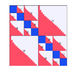
Figure 3: Hierarchical low-rank structure of the 1D fractional Laplace operator discretized through Grünwald-Letnikov finite differences. The blue blocks are dense, while the gray blocks are stored as low-rank matrices whose rank is indicated by the number in the center. In red, the magnitude of the singular values of the low-rank blocks.

In the next section we will investigate how varying this parameter affects the performances.

We consider increasing sizes $n=2^{j}$, $j=10,\dots,15$ and the following solvers:

diag

Algorithm 1 with explicit diagonalization of the matrix $A$ performed in dense arithmetic.

dst

Algorithm 1 incorporating the fast diagonalization by means of the Discrete Sine Transform (DST). This approach is only considered for the 2D Laplace equation.

superdc

solver implementing Algorithm 1 using the fast diagonalization for SPD HSS matrices described in [ou2022superdc].

dc_adi

Algorithm 3 where the fADI iteration is used as low_rank_sylv.

dc_rk

Algorithm 3 where the rational Krylov method is used as low_rank_sylv.

dc_ek

Algorithm 3 where the extended Krylov method is used as low_rank_sylv.

The shifts used in dc_adi and dc_rk are the optimal Zolotarev zeros and poles. The number of shifts is chosen to obtain similar residual norms $\mathrm{Res}:=\lVert A\widetilde{X}+\widetilde{X}A-B\rVert_{F}/\lVert B\rVert_{F}$ of about $10^{-10}$.

We start by comparing the different implementation of Algorithm 3 with diag. A detailed comparison with dst and superdc is postponed to Section LABEL:sec:superdc.

The running times and residuals are reported in Table LABEL:tab:2d-laplace for the Laplace equation. The fractional case is reported in Table LABEL:tab:2d-fractional, for which we do not report the timings for $n=1024,2048$ since our choice of $n_{\min}$ makes Algorithm 3 equivalent to Algorithm 1.

For both experiments, using fADI as low-rank solver yields the cheapest method. We remark that, in the fractional case, dc_ek outperforms dc_rk since the precomputation of the Cholesky factorization of $A$ (and of its sub blocks) makes the iteration of extended Krylov significantly cheaper than the one of rational Krylov.

In Figure LABEL:fig:hist_2D_Laplace and LABEL:fig:hist_2D_Fractional_Laplace we display how the time is distributed among the various subtasks of dc_adi, i.e., the time spent on solving dense matrix equations, computing the low-rank updates, forming the RHS of the update equation and updating the solution, and estimating the spectra.