FedCliP: Federated Learning with Client Pruning

Abstract

The prevalent communication efficient federated learning (FL) frameworks usually take advantages of model gradient compression or model distillation. However, the unbalanced local data distributions (either in quantity or quality) of participating clients, contributing non-equivalently to the global model training, still pose a big challenge to these works. In this paper, we propose FedCliP, a novel communication efficient FL framework that allows faster model training, by adaptively learning which clients should remain active for further model training and pruning those who should be inactive with less potential contributions. We also introduce an alternative optimization method with a newly defined $contribution\ score$ measure to facilitate active and inactive client determination. We empirically evaluate the communication efficiency of FL frameworks with extensive experiments on three benchmark datasets under both IID and non-IID settings. Numerical results demonstrate the outperformance of the porposed FedCliP framework over state-of-the-art FL frameworks, i.e., FedCliP can save 70% of communication overhead with only 0.2% accuracy loss on MNIST datasets, and save 50% and 15% of communication overheads with less than 1% accuracy loss on FMNIST and CIFAR-10 datasets, respectively.

1 Introduction

Federated learning (FL) generates an effective global model by training local models independently on each client and aggregating local model parameters on a central server while preserving data privacy McMahan et al. (2017); Li et al. (2020a, 2021); Karimireddy et al. (2020); Shoham et al. (2019). Despite the FL schemes’ success, the FL training methods still suffer from high communication costs because clients are usually equipped with limited hardware resources and network bandwidth, which suspend the deployment of large neural networks on a wide scale. Communication efficiency is a significant bottleneck restricting the development and deployment of FL.

Various works have been proposed to solve the communication bottleneck, and we can divide these methods into four categories: (1) Accelerated model convergence techniques Cho et al. (2020); Goetz et al. (2019); Xu et al. (2022); Tang et al. (2022); Wang et al. (2022) reduce the overall communication cost by reducing the number of communication rounds required for global model convergence, (2) compression techniques Fu et al. (2020); Stich et al. (2018); Hyeon-Woo et al. (2021); Sun et al. (2022) that utilize fewer bits to represent gradients or parameters to reduce communication costs, (3) model pruning techniques Jiang et al. (2019); Bao et al. (2022) that identify much smaller sub-networks to reduce the communication overhead. And (4) knowledge distillation Wu et al. (2022); Lin et al. (2020) techniques allow the server to extract client knowledge.

The works mentioned above achieve communication efficiency from the point of view of compressing model parameters or searching for critical parameters or vital structures of the client model. However, the unbalanced local data distributions of participating clients, contributing non-equivalently to the global model convergence, still pose a significant challenge to these works. When the client model or data does not contribute to the global model training, even if the above communication efficient methods are used, the overhead of model communication will still be incurred because these methods will not discard all the client model parameters. Our key idea is mainly based on the following intuitions:

Clients do not contribute equivalently. Training clients with a large and balanced dataset can be more beneficial to the convergence of the global model, while training clients with small and highly biased datasets may increase the losses of the global model. The local model convergence rate is inconsistent, caused by data imbalance. A client participates in global training many times, the local model tends to converge gradually, and its contribution to the global model will decrease progressively. It will occupy valuable model training resources and harm model convergence if this client still participates in the training.

This means we should pay more attention to those have more effect on global model convergence to participate in training, and clients with less contribution even play a negative role will be pruned gradually with the FL training. In this paper, we propose a client-pruning strategy, FedCliP, that can quickly identify essential active clients through several communication rounds and progressively reduce the inactive clients participating in FL training. The pruned inactive clients will no longer participate in the following training process. Screening essential clients during the FL training process narrows the scope of participating in training clients continuously, and achieves communication efficiency from the macro perspective of the FL framework. Our contributions in this paper are summarized as follows:

• We propose the first communication efficient FL framework with client pruning based on our knowledge, dubbed FedCliP, which can identify active clients that contribute more to the global model and minimize communication overhead by excluding inactive clients that contribute less to global model training from the FL training process.

• We define a client $contribution\ score$ measure to promote active and inactive client decisions. The client $contribution\ score$ can adaptively evaluate the contribution value of the client in this round, measure each client’s data quality and model difference, and fully utilizes each client’s resources.

• We introduce an alternative optimization method to determine the next round of active client sets. We utilize Gaussian Scale Mixture (GSM) modeling to model the client $contribution\ score$, efficiently estimate the numerical components of active clients, and then realize the screening of inactive clients.

• We have conducted numerous experiments on three benchmark datasets under IID and non-IID settings. The numerical results show that the proposed FedCliP can save 70% of the communication overhead, only 0.2% of the accuracy is lost on the MNIST dataset, and 50% and 15% of the communication overhead are saved, with less than 1% of the accuracy loss on the FMNIST and CIFAR-10 datasets, respectively.

2 Related Works

2.1 Federated Learning

Federated Learning (FL) enables participating clients to collaboratively train a model without migrating the client’s data, which addresses privacy concerns in a distributed learning environment Li et al. (2020b); Dinh et al. (2021); Liu et al. (2021); Arivazhagan et al. (2019); Liang et al. (2020); Shamsian et al. (2021); Luo and Wu (2022). FedAvg McMahan et al. (2017) is the the most widely used FL algorithm. In FedAvg framework, the server sends the initial parameters to the participating clients. The parameters are updated independently on each of these clients to minimize the local data loss, and the locally trained parameters are sent to the server. The server aggregates the local parameters by simply averaging them and obtains the next round of global parameters. Many studies focus on amending the local model updates or the central aggregation based on FedAvg. FedProx Li et al. (2020a) is another notable FL framework that stabilizes FedAvg by including a proximal term in the loss function to limit the distance between local and global models. FedReg Xu et al. (2022) proposed to encode the knowledge of previous training data learned by the global model and accelerate FL with alleviated knowledge forgetting in the local training stage by regularizing locally trained parameters with the loss on generated pseudo data.

2.2 Communication Efficient Federated Learning

Fruitful literature has studied model compression to reduce communication costs in distributed learning. The basic idea of these methods is that before uploading the trained local model to the server, first compress and encode the model parameters or gradients, and then the communication is efficient by uploading a small amount of data. Compression on server-to-client communication is non-trivial and attracted many recent focuses Hyeon-Woo et al. (2021); Fu et al. (2020); Stich et al. (2018). Pruning and distillation methods have been combined with federated learning to achieve model compression in recent years Zhang et al. (2022); Alizadeh et al. (2022); Jiang et al. (2019); Wu et al. (2022); Lin et al. (2020). Model pruning removes inactive weights to address the resource constraints, and model distillation requires a student model to mimic the behavior of a teacher model. These methods aim to find important model parameters or structures and achieve communication efficiency by transferring essential parts of the model. In addition, the way to achieve efficient federated learning communication is to speed up the convergence of the model Xu et al. (2022). Because the convergence of the global model is faster, the required communication rounds will be reduced accordingly, and the communication costs will be reduced accordingly. However, they did not consider the impact of the unbalanced distribution of client data on the global model training. When the client model has no contribution to the global model training, the above methods cannot achieve real communication efficiency because they cannot discard all the local model parameters in principle. The FedCliP method proposed in this paper can adaptively prune the client during the model training process, and the pruned client cannot continue to participate in the federated learning process, thus reducing the communication overhead to the greatest extent.

3 Methodology

In this section, we elaborate our proposed FL framework, i.e., FedCliP, that can achieve communication efficient. We first introduce the goal of our FedCliP framework in Section 3.1. Then, the client $contribution\ score$ calculation method is given in Section 3.2, based on the data quality and model difference. Then, we provide empirical evidence that the prior distribution of client $contribution\ score$ in each communication round can be modeled as Gaussian distribution. Based on this observation, we utilize GSM to model the client pruning problems in Section 3.3 and obtain an effective client pruning optimization strategy for FL in Section 3.4. We illustrate the framework of FedCliP in Figure 1.

3.1 Problem Formulation

In the FL, the client $k$ keeps its local data $\mathbb{D}_{k}$ on the client machine during the whole training process. FL aims to seeks for a global model $\bm{w}$ that achieves the best performance on all $N$ clients. We refer to $l_{k}(\bm{w})$ as the local loss of client $k$, which is evaluated with the local dataset $\mathbb{D}_{k}$, which size is $\left|\mathbb{D}_{k}\right|$, on client $k$. The weight $p_{k}=\left|\mathbb{D}_{k}\right|/\sum_{j}\left|\mathbb{D}_{j}\right|$ of the client $k$ is proportional to the size of its local dataset.

In this paper, in communication round $t$, we select the overall clients in client set $\mathbb{U}_{t}$ to receive the global model $\bm{w}^{t}$ and conduct training with their local dataset for several iterations independently. After the local training, the server collects the trained models from these selected clients and aggregates them to produce a new global model $\bm{w}^{t+1}$. Our goal is to dynamically evaluate the $contribution\ score$ of each client during the FL process and determine whether the client will continue to participate in the next training round based on the $contribution\ score$. Clients who can continue participating in the following training round will constitute a new collection of clients $\mathbb{U}_{t}$ for $t+1$ communication rounds.

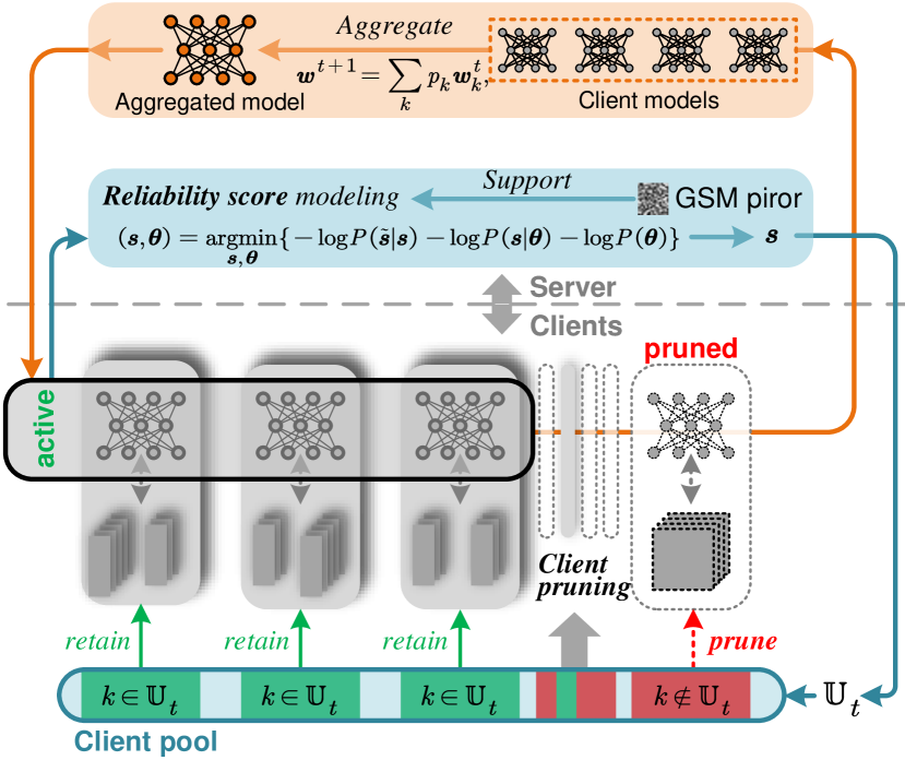
Figure 1: The framework of the proposed FedCliP. The server utilizes the GSM to model the $contribution\ score$ calculated by each client and updates the set of active clients participating in the next round of training.

3.2 Contribution Score

To effectively identify inactive clients, we measure each client’s model with the $contribution\ score$, which jointly considers the contribution of the local model and data quality to the global model. After the client receives the global model and completes local training, the difference between the current local model and the global model is an essential indicator for judging whether the client needs to continue to participate in the next round of training. A slight difference value means that the client data contributes less to the convergence of the global model, and the probability of the client continuing to participate in training is lower. Similarly, as the training proceeds, the local model of an active client and the updated global model has a relatively large distance. The model difference is an effective metric to quantify the model quality in FL. Based on this point of view, we define the model difference below.

Definition 1.

We define the model difference $d$ for the $k$-th client as the $\ell_{2}$-norm distance between the current local model $\bm{w}_{k}^{t}$ and last-round global model $\bm{w}^{t-1}$, i.e.

$$\small d_{k}^{t}=\left\|\bm{w}_{k}^{t}-\bm{w}^{t-1}\right\|_{2}^{2},$$ (1)

As the most critical resource for the client, data quality is another important criterion for measuring the client’s contribution. Clients with high-quality data often need to continue participating in the federated learning process because high-quality data will positively affect the convergence of the global model. However, data quality has always been challenging to evaluate and predict. To measure client data quality, we quantify data quality from two aspects: the convergence speed of the local model on the client data and the amount of data. We utilize the local model’s training loss to measure the local model’s convergence speed. The data size is often used to evaluate the client data quality, and we continue to use this point of view. Overall, we define the client’s data quality below.

Definition 2.

We define the data quality $q$ for the $k$-th client using the client training loss of the local training data and the data size, i.e.

$$\small q_{k}^{t}=\left|\mathbb{D}_{k}\right|\sqrt{\frac{1}{\mathbb{D}_{k}}\sum_{d\in\mathbb{D}_{k}}l_{k}(\bm{w}_{k}^{t},d)^{2}}.$$ (2)

At last, we integrate the model difference of Eq. (1) and local data quality of Eq. (2) into our $contribution\ score$, and we define the $contribution\ score$ below.

Definition 3.

We define the $contribution\ score$ $s$ for the $k$-th client using the model difference and local data quality, i.e.

$$\small s_{k}^{t}=d_{k}^{t}*q_{k}^{t}.$$ (3)

As an important indicator to judge whether the current client continues to participate in the federated learning process, the $contribution\ score$ makes full use of the information of the local model and data and plays a vital role in dynamically pruning the client.

3.3 Gaussian Scale Mixture Modeling for Contribution Scores

After getting the $contribution\ score$ of each client, we can pruning the inactive clients with $contribution\ scores$ $\bm{s}^{t}=\left\{s_{1}^{t},\ldots s_{N}^{t}\right\}$ obtained in communication round $t$. We regard identifying inactive clients from the $contribution\ scores$ of all clients as a data-denoising task. By considering the $contribution\ scores$ of inactivate clients as Gaussian noise of clean $contribution\ scores$ of all clients, we utilize the GSM to model the $contribution\ scores$ and obtain the clean $contribution\ scores$ representing the active clients. For simplicity, we set $\tilde{\bm{s}}\in\mathbb{R}^{N}$ and $\bm{s}\in\mathbb{R}^{N}$ denote the one-dimensional representations of all clients’ $contribution\ scores$ and activate clients’ $contribution\ scores$, respectively. Then $\bm{s}$ denotes the noiseless version of $\tilde{\bm{s}}$, i.e., $\tilde{\bm{s}}=\bm{s}+\bm{n}$, where $\bm{n}\in\mathbb{R}^{N}$ denotes additive Gaussian noise of inactive clients’ $contribution\ scores$. In this subsection, we propose a Maximum A Posterior (MAP) method for estimating $\bm{s}$ from $\tilde{\bm{s}}$, and the MAP estimation of $\bm{s}$ from $\tilde{\bm{s}}$ can be formulated as

$$\small\bm{s}=\mathop{\arg\min}_{\bm{s}}\{-\log P(\tilde{\bm{s}}|\bm{s})-\log P(\bm{s})\},$$ (4)

where $\log P(\tilde{\bm{s}}|\bm{s})$ is given by the Gaussian distribution of noise from inactive clients, i.e.,

$$\small P(\tilde{\bm{s}}|\bm{s})\propto\exp\left(-\frac{1}{2\sigma_{w}^{2}}\|\tilde{\bm{s}}-\bm{s}\|_{2}^{2}\right),$$ (5)

where $\exp(\cdot)$ denotes the exponential operation on each element of the input parameters, and $\sigma_{w}^{2}$ is the variance of the Gaussian noise. A prior distribution of $\bm{s}$ is given by Laplacian, and it is easy to verify that the above MAP estimation leads to the following weighted $\ell_{1}$-norm minimization problem when $P(\bm{s})$ is chosen to be an IID Gaussian,

$$\small\bm{s}=\mathop{\arg\min}_{\bm{s}}\|\tilde{\bm{s}}-\bm{s}\|_{2}^{2}+2\sigma_{w}^{2}\sum_{j}\frac{1}{\theta_{j}}\left|s_{j}\right|,$$ (6)

where $\theta_{j}$ denotes the standard derivation of $s_{j}$. In realistic scenarios, it is difficult to estimate the $\theta_{j}$ from $\tilde{\bm{s}}$. The right side of Figure 3 shows the probability distribution of all client $contribution\ scores$ after completing the training. It can be seen that during the dynamic training process, the distribution of client $contribution\ scores$ roughly satisfies the Gaussian distribution. It can also be explained from the side of the rationality of our setting of $contribution\ score$ measure.

In this paper, we propose a Gaussian Scale Mixture (GSM) prior for $\bm{s}$. GSM model has demonstrated its potential for signal modeling in computer vision works Fang et al. (2022); Lu et al. (2022); Huang et al. (2021); Ning et al. (2020); Shao et al. (2021). With the GSM prior, one can decompose $\bm{s}$ into point-wise product of a Gaussian vector $\bm{\alpha}$ and a positive hidden scalar multiplier $\bm{\theta}$ with probability $P\left(\theta_{j}\right)$, i.e., $s_{i}=\theta_{j}\alpha_{j}$. Conditioned on $\theta_{j}$, $s_{j}$ is Gaussian with standard deviation $\theta_{j}$, assuming that $\theta_{j}$ and $\alpha_{j}$ are independently identically distribution (IID), we can write the GSM prior of $\bm{s}$ as

$$\small P(\bm{s})=\prod_{j}P\left(s_{j}\right),P\left(s_{j}\right)=\int_{0}^{\infty}P\left(s_{j}|\theta_{j}\right)P\left(\theta_{j}\right)d\theta_{j}.$$ (7)

Then, we compute the MAP estimation of $\bm{s}$ with the GSM prior by using a joint prior model $P\left(\bm{s},\bm{\theta}\right)$. By substituting $P\left(\bm{s},\bm{\theta}\right)$ into the MAP estimation of Eq. (4), we can obtain

$$\small(\bm{s},\bm{\theta})=\mathop{\arg\min}_{\bm{s},\bm{\theta}}\{-\log P(\tilde{\bm{s}}|\bm{s})-\log P(\bm{s}|\bm{\theta})-\log P(\bm{\theta})\}.$$ (8)

Here we adopt the noninformative Jeffrey’s prior Box and Tiao (1992), i.e., $P\left(\theta_{j}\right)=1/\theta_{j}$, and Eq. (8) can be written into

$$\small(\bm{s},\bm{\theta})=\mathop{\arg\min}_{\bm{s},\bm{\theta}}\|\tilde{\bm{s}}-\bm{s}\|_{2}^{2}+\sigma_{w}^{2}\sum_{j}\frac{s_{j}^{2}}{\theta_{j}^{2}}+4\sigma_{w}^{2}\sum_{j}\log\theta_{j}.$$ (9)

Note that in GSM we have $\bm{s}=\bm{\Lambda}\bm{\alpha}$, where $\bm{\Lambda}=\operatorname{diag}\left(\theta_{j}\right)\in\mathbb{R}^{N\times N}$. Then Eq. (9) can be rewritten as

$$\small\begin{split}(\bm{\alpha},\bm{\theta})=&\mathop{\arg\min}_{\bm{s},\bm{\theta}}\|\tilde{\bm{s}}-\bm{\Lambda}\bm{\alpha}\|_{2}^{2}+\sigma_{w}^{2}\|\bm{\alpha}\|_{2}^{2}\\ &+4\sigma_{w}^{2}\sum_{j}\log\left(\theta_{j}+\epsilon\right),\end{split}$$ (10)

where $\epsilon$ is a small positive constant. From Eq. (10), we can see that the estimation of $\bm{s}$ has been translated into the joint estimation of $\bm{\alpha}$ and $\bm{\theta}$.

Algorithm 1 Client Pruning Strategy

Require: Active client set $\mathbb{U}_{t}$, $contribution\ scores$ $\tilde{\bm{s}}^{t}$, $\sigma_{w}^{2}$
Ensure: Active client set $\mathbb{U}_{t+1}$

1:  Initialize $\mathbb{U}_{t+1}\leftarrow\emptyset$.

2:  while not converged do

3:     Compute $\bm{\theta}^{t}$ using Eq. (11).

4:     Compute $\bm{\alpha}^{t}$ using Eq. (16).

5:     Compute $\bm{A}^{t}=\operatorname{diag}\left(\bm{\alpha}^{t}\right)$, $\bm{s}^{t}=\bm{A}^{t}\bm{\theta}^{t}$.

6:  end while

7:  for each client $k\in\mathbb{U}_{t}$ do

8:     Set corresponding value of $k$ in $\bm{s}^{t}$ is $\bm{s}_{k}^{t}$.

9:     if $\bm{s}_{k}^{t}>0$ then

10:        Add $k$ into $\mathbb{U}_{t+1}$ and remove it from $\mathbb{U}_{t}$.

11:     end if

12:  end for

13:  return $\mathbb{U}_{t+1}$

3.4 Alternative Optimization

We propose an efficient algorithm solving Eq. (10) by an alternating minimization, and we describe each sub-problem as follows.

3.4.1 Solving the $\bm{\theta}$ Subproblem

When the $\bm{\alpha}$ is fixed, we can solve for $\bm{\theta}$ by optimizing

$$\small\bm{\theta}=\mathop{\arg\min}_{\bm{\theta}}\|\tilde{\bm{s}}-\bm{A}\bm{\theta}\|_{2}^{2}+4\sigma_{w}^{2}\sum_{j}\log\left(\theta_{j}+\epsilon\right),$$ (11)

where $\bm{A}=\operatorname{diag}\left(\bm{\alpha}\right)$, and $\bm{\Lambda}\bm{\alpha}=\bm{A}\bm{\theta}$. Equivalenty, Eq. (11) can be rewritten as

$$\small\bm{\theta}=\mathop{\arg\min}_{\bm{\theta}}\sum_{j}\left\{a_{j}\theta_{j}^{2}+b_{j}\theta_{j}+c\log\left(\theta_{j}+\epsilon\right)\right\},$$ (12)

where $a_{j}=\alpha_{j}^{2}$, $b_{j}=-2\alpha_{j}\tilde{s_{j}}$ and $c=4\sigma_{w}^{2}$. Thus, Eq. (12) boils down to solving a sequence of scalar minimization problems

$$\small\theta_{j}=\mathop{\arg\min}_{\bm{\theta_{j}}}a_{j}\theta_{j}^{2}+b_{j}\theta_{j}+c\log\left(\theta_{j}+\epsilon\right),$$ (13)

which can be solved by taking $df(\theta_{j})/d\theta_{j}=0$, where $f(\theta)$ denotes the right hand side of Eq. (13). By taking $df(\theta_{j})/d\theta_{j}=0$, two stationary points can be obtained

$$\small\theta_{j,1}=-\frac{b_{j}}{4a_{j}}+\sqrt{\frac{b_{j}^{2}}{16}-\frac{c}{2a_{j}}},\theta_{j,2}=-\frac{b_{j}}{4a_{j}}-\sqrt{\frac{b_{j}^{2}}{16}-\frac{c}{2a_{j}}},$$ (14)

then we denote $\Delta=b_{j}^{2}/\left(16a_{j}^{2}\right)-c/\left(2a_{j}\right)$, the solution to Eq. (14) can then be written as

$$\small\theta_{j}=\begin{cases}0&,\text{if $\Delta<0$}\\ t_{j}&,\text{otherwise}\text{,}\end{cases}$$ (15)

where $t_{j}=\mathop{\arg\min}_{\theta_{j}}\left\{f(0),f\left(\theta_{j,1}\right),f\left(\theta_{j,2}\right)\right\}$.

Algorithm 2 FedCliP

Server executes:

1:  Initialize global model $\bm{w}^{0}$, active client set $\mathbb{U}_{0}\leftarrow\mathbb{P}$.

2:  for each round $t=0,1,\ldots$ do

3:     Select all clients $\bm{S}_{t}$ from $\mathbb{U}_{t}$.

4:     for each client $k\in\bm{S}_{t}$ in parallel do

5:        $\bm{w}_{k}^{t+1},s_{k}^{t}\leftarrow\text{ClientUpdate}\left(k,\bm{w}^{t}\right)$.

6:     end for

7:     $\bm{w}^{t+1}\leftarrow\sum_{k\in\bm{S}_{t}}p_{k}\bm{w}_{k}^{t+1}$.

8:     Collect select clients $contribution\ scores$ $\tilde{\bm{s}}^{t}$.

9:     Update active client set $\mathbb{U}_{t+1}\leftarrow\mathbb{U}_{t}$ with Algorithm 1.

10:  end for

ClientUpdate($k$, $\bm{w}$):

1:  Initialize the number of local epochs $E$, local minibatch size $B$, learning rate $\eta$.

2:  $\mathcal{B}\leftarrow$ (split $\mathbb{D}_{k}$ into batches of size $B$).

3:  for each local epoch $i$ from 1 to $E$ do

4:     for batch $b\in\mathcal{B}$ do

5:        $\bm{w}\leftarrow\bm{w}-\eta\nabla l_{k}\left(\bm{w};b\right)$

6:     end for

7:  end for

8:  Calculate $contribution\ score$ $s$ using Eq. (3).

9:  return $\bm{w}$ and $s$ to server

3.4.2 Solving the $\bm{\alpha}$ Subproblem

For fixed $\bm{\theta}$, $\bm{\alpha}$ can be updated by solving

$$\small\bm{\alpha}=\mathop{\arg\min}_{\bm{\alpha}}\|\tilde{\bm{s}}-\bm{\Lambda}\bm{\alpha}\|_{2}^{2}+\sigma_{w}^{2}\|\bm{\alpha}\|_{2}^{2},$$ (16)

which also admits a closed-form solution namely

$$\small\bm{\alpha}=\left(\bm{\Lambda}^{\top}\bm{\Lambda}+\sigma_{w}^{2}\bm{I}\right)^{-1}\bm{\Lambda}^{\top}\tilde{\bm{s}},$$ (17)

where $\bm{I}$ denotes the identity matrix. Since $\left(\bm{\Lambda}^{\top}\bm{\Lambda}+\sigma_{w}^{2}\bm{I}\right)$ is a diagonal matrix, Eq. (17) can be easily computed.

By alternatingly solving the sub-problems of Eq. (11) and Eq. (16), sparse coefficients $\bm{s}$ can be estimated as $\hat{\bm{s}}=\hat{\bm{\Lambda}}\hat{\bm{\alpha}}$, where $\hat{\bm{\Lambda}}$ and $\hat{\bm{\alpha}}$ denote the estimates of $\bm{\Lambda}$ and $\bm{\alpha}$ respectively. At last, the clients corresponding to the non-zero values in $\bm{s}$ are the active clients when we obtain the active clients’ $contribution\ scores$ $\bm{s}$. In summary, the proposed GSM-based client pruning strategy is summarized in Algorithm 1, and the overall framework FedCliP based on Algorithm 1 is summarized in Algorithm 2. It is noteworthy that our method is orthogonal to existing FL optimizers that amend the training loss or the aggregation scheme, e.g., FedAvg McMahan et al. (2017) and FedProx Li et al. (2020a). So our method can be combined with any of them.

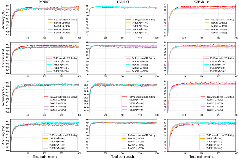
Figure 2: The test accuracy achieved by FedCliP on MNIST, FMNIST and CIFAR-10 under IID and non-IID settings.

4 Experiments

4.1 Experimental Setup

Benchmark Datasets. We conduct experiments on three classical datasets, including MNIST Deng (2012), FMNIST Xiao et al. (2017) and CIFAR-10 Krizhevsky et al. (2009). For MNIST, we adopt a CNN model with two convolutional layers followed by two linear layers. For FMNIST and CIFAR-10, we adopt the ResNet18 model with five convolutional layers followed by one linear layer. We partition each dataset into a training set and a test set with the same distributions, and transform the datasets according to IID distribution, and ensure the same distributions of local training and test set. We experiment with two different data partitions on N = 20 clients as follows.

IID and non-IID Settings. We design two data distributions for empirical evaluation, IID setting and non-IID setting. For IID setting, each client distributes data equally to ensure consistent data distribution on each client. For non-IID setting, to simulate the data distribution more realistically, we randomly select 80% of the data, distribute them to 10 clients according to the IID method. Then, we divide the remaining data into 20 shards ensuring that all the data in one shard have same label, and distribute them to the other 10 clients so that each client has two shards.

Baseline Studies. We implement FedCliP following two state-of-the-art FL approaches to verify the feasibility and effectiveness of client pruning strategy: (1) FedAvg McMahan et al. (2017), which takes the average of the locally trained copies of the global model; (2) FedProx Li et al. (2020a), which stabilizes FedAvg by including a proximal term in the loss function to limit the distance between the local model and last round global model.

Parameter Settings. We train each method 200 communication rounds with 5 local epochs on each datasets. The client pruning ratio $\lambda$ on the MNIST datasets, we set $\lambda=$ 10%, 30%, 50%, and 70%, respectively. For FMNIST dataset, we set $\lambda=$ 10%, 20%, 30% and 50%, respectively. We set $\lambda=$ 10%, 15%, 20% and 30% on the CIFAR-10 dataset. During the experiment, due to the instability of model training in the first 20 communication rounds, we did not perform client pruning operations in the first 20 rounds and pruned a client in each training round after the first 20 rounds.

4.2 Experimental Results under IID Setting

We summarize the empirical convergence behavior and performance under the IID and non-IID settings in Tables 1, 2, 3 and Figure 2. The test accuracy curves of the total training rounds are shown in Figure 2, from which we can see that, under all experimental settings, all experimental training results can converge stably to a certain exact value, which means that using the FedCliP client pruning strategy can bring the federated training model to convergence.

Corresponding to the IID setting, the FedCliP method performs best on the MNIST data set. Although the FedAvg and FedProx methods both achieve optimal performance without any client pruning, we can see from Table 1 that when using FedCliP to dynamically prune clients during FL model training, even if the pruning rate is up to 70%, the global model performance only drops by 0.2%, still, the overall communication cost of the entire FL model has decreased by about 70%. The experimental results on the FMNIST dataset show that as the client pruning rate increases, the overall performance of the global model shows a downward trend, which is a very intuitive and natural phenomenon. One can see from Table 2 that when the rate reaches 50%, the model’s performance only drops by 1%, but the communication consumption at this time is reduced by 50%. As shown in Table 3, when we set the client pruning rate to be around 15% to 20%, we can control the model accuracy decrease of the FedCliP algorithm within 1%, which means that the use of an acceptable model loss can maximize the reduction in communication consumption.

4.3 Experimental Results under non-IID Setting

For non-IID setting, we find an interesting phenomenon in Table 1: the accuracy results of dynamically pruning 30% of clients using the FedCliP strategy are the best on MNIST dataset, compared with the original method without any client pruning effects better. In the case of using all clients to participate in training, the data distributed on half of the clients is unbalanced, which accounts for 20% of all train data and may harm the gradient descent of the model. Utilizing the method of dynamically pruning clients can effectively screen clients unfavorable to model convergence so that they do not continue to participate in the training of the global model, stabilizing the training results and minimizing communication overhead. The experimental results in Table 2 can also verify our statement. The performance of the FedProx using the client pruning strategy is higher than the original method without any client pruning. When the pruning rate reaches 50%, the model performance is still slightly higher than the effect of not adopting the pruning strategy. The experimental results on the CIFAR-10 dataset in Table 3 prove that the FedProx using the client pruning strategy can reduce the communication cost of FL without losing the model’s accuracy.

4.4 Ablation Study

The ablation experiments are designed to show the effectiveness of each component of $contribution\ score$ to the performance, ablation experiment results are shown in Figure 3. The critical indicator of the FedCilP dynamic pruning client is the $contribution\ score$ calculated by each client after the current round of local training. The calculation of the $contribution\ score$ consists of two parts, the model difference, and the data quality. The experimental results in Figure 3 confirm the correctness of the pruning evaluation index we set. We only use model difference and data quality as a $contribution\ score$ standard, and the expected results can be obtained. We combine the two as the evaluation criteria for the FedCliP dynamic pruning client to improve the results.

4.5 Results Discussion

As a novel solution to reduce the communication overhead, during the model training process, FedCliP gradually identifys active clients and prunes inactive clients. By setting up two more classic experimental scenarios, we verified the necessity and feasibility of gradually pruning the client during the FL process and reduced the communication overhead of the model as much as possible under the accuracy loss controllable. From IID setting, when we use FedCliP to dynamically prune clients during FL model training, even if the pruning rate is up to 70%, the global model performance only drops by 0.2%, still, the overall communication cost of the entire FL model has decreased by about 70%. The non-IID setting can better reflect the performance superiority of the FedCliP algorithm. Due to the balanced distribution of some client data under the non-IID setting, it can easily lead to unstable model training. Through adaptive pruning clients during the model training process, accurately pruning inactive clients and retaining active clients can improve the stability of model training. Utilizing the method of dynamically pruning clients can effectively screen clients unfavorable to model convergence so that they do not continue to participate in the training of the global model, stabilizing the training results and minimizing communication overhead.

Method		Accuracy		Communication costs
		IID	non-IID
FedAvg		$\bm{99.25}$	99.16	1.00
FedCliP	10%	99.14	99.18	0.90
	30%	99.21	$\bm{99.25}$	0.70
	50%	99.11	99.15	0.50
	70%	99.05	99.25	0.30
FedProx		$\bm{99.25}$	99.22	1.00
FedCliP	10%	99.14	99.19	0.90
	30%	99.12	$\bm{99.25}$	0.70
	50%	99.19	99.15	0.50
	70%	99.13	99.06	0.30

Table 1: Best test accuracy (%) achieved by FedCliP on MNIST dataset under IID and non-IID settings. Highest performance is represented in bold.

Method		Accuracy		Communication costs
		IID	non-IID
FedAvg		92.50	92.36	1.00
FedCliP	10%	92.05	92.32	0.90
	20%	$\bm{92.73}$	$\bm{92.37}$	0.80
	30%	92.05	92.20	0.70
	50%	91.51	92.25	0.50
FedProx		$\bm{92.43}$	92.24	1.00
FedCliP	10%	92.37	92.27	0.90
	20%	92.43	$\bm{92.43}$	0.80
	30%	91.76	92.16	0.70
	50%	91.54	92.02	0.50

Table 2: Best test accuracy (%) achieved by FedCliP on FMNIST dataset under IID and non-IID settings. Highest performance is represented in bold.

Method		Accuracy		Communication costs
		IID	non-IID
FedAvg		$\bm{82.22}$	$\bm{83.01}$	1.00
FedCliP	10%	80.92	82.04	0.90
	15%	81.37	82.21	0.85
	20%	80.32	82.14	0.80
	30%	80.66	81.87	0.70
FedProx		$\bm{81.98}$	81.88	1.00
FedCliP	10%	80.78	82.24	0.90
	15%	81.39	$\bm{82.60}$	0.85
	20%	81.05	81.83	0.80
	30%	80.43	82.22	0.70

Table 3: Best test accuracy (%) achieved by FedCliP on CIFAR-10 dataset under IID and non-IID settings. Highest performance is represented in bold.

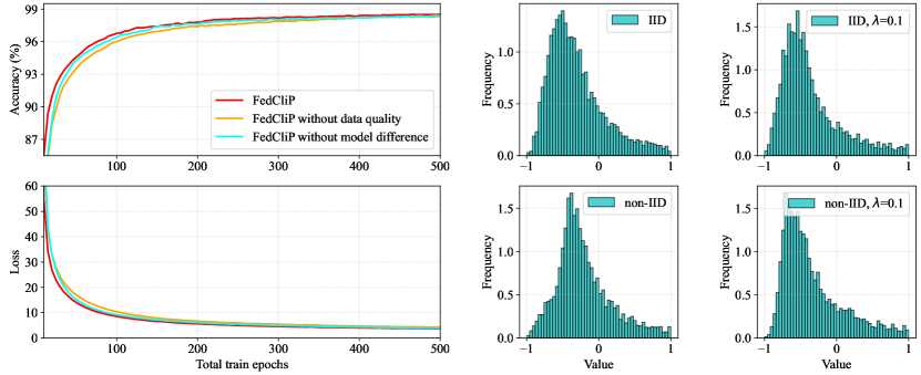
Figure 3: Left: the test accuracy and loss achieved by FedCliP ($\lambda=0.6$) on MNIST under IID setting. Right: the distributions of $contribution\ scores$ achieved by FedCliP on MNIST dataset.

5 Conclusion and Future Work

In this paper, we propose a novel FL framework for communication efficiency, named FedCliP, by adaptively learning which clients should remain active for next round model training and pruning those clients that should be inactive and have less potential contribution. We also introduced an alternative optimization method based on GSM modeling, using a newly defined $contribution\ score$ metric to help identify active and inactive clients. We empirically evaluate the communication efficiency of the FL framework by conducting extensive experiments on three benchmark datasets under IID and non-IID settings. Numerical results show that the proposed FedCliP framework outperforms the state-of-the-art FL framework for efficient communication, i.e., FedCliP can save 70% of communication overhead with only 0.2% accuracy loss on MNIST dataset, and save 50% on FMNIST and 15% on CIFAR-10 communication overhead, respectively, with an accuracy loss of less than 1%. In our future work, we will consider the client recycling mechanism to enhance the performance of our proposed algorithm further.

References

- Alizadeh et al. [2022] Milad Alizadeh, Shyam A. Tailor, Luisa M Zintgraf, Joost van Amersfoort, Sebastian Farquhar, Nicholas Donald Lane, and Yarin Gal. Prospect pruning: Finding trainable weights at initialization using meta-gradients. In International Conference on Learning Representations, 2022.
- Arivazhagan et al. [2019] Manoj Ghuhan Arivazhagan, Vinay Aggarwal, Aaditya Kumar Singh, and Sunav Choudhary. Federated learning with personalization layers. arXiv preprint arXiv:1912.00818, 2019.
- Bao et al. [2022] Yajie Bao, Michael Crawshaw, Shan Luo, and Mingrui Liu. Fast composite optimization and statistical recovery in federated learning. In International Conference on Machine Learning, volume 162, pages 1508–1536. PMLR, 2022.
- Box and Tiao [1992] George E. P. Box and George C. Tiao. Bayesian Inference in Statistical Analysis. Boston, MA, USA: Addison-Wesley, 1992.
- Cho et al. [2020] Yae Jee Cho, Jianyu Wang, and Gauri Joshi. Client selection in federated learning: Convergence analysis and power-of-choice selection strategies. arXiv preprint arXiv:2010.01243, 2020.
- Deng [2012] Li Deng. The mnist database of handwritten digit images for machine learning research. IEEE Signal Processing Magazine, 29(6):141–142, 2012.
- Dinh et al. [2021] Canh T Dinh, Tung T Vu, Nguyen H Tran, Minh N Dao, and Hongyu Zhang. Fedu: A unified framework for federated multi-task learning with laplacian regularization. arXiv preprint arXiv:2102.07148, 2021.
- Fang et al. [2022] Zhenxuan Fang, Weisheng Dong, Xin Li, Jinjian Wu, Leida Li, and Guangming Shi. Uncertainty learning in kernel estimation for multi-stage blind image super-resolution. In European Conference on Computer Vision, pages 144–161, 2022.
- Fu et al. [2020] Fangcheng Fu, Yuzheng Hu, Yihan He, Jiawei Jiang, Yingxia Shao, Ce Zhang, and Bin Cui. Don’t waste your bits! squeeze activations and gradients for deep neural networks via tinyscript. In International Conference on Machine Learning, volume 119, pages 3304–3314. PMLR, 2020.
- Goetz et al. [2019] Jack Goetz, Kshitiz Malik, Duc Bui, Seungwhan Moon, Honglei Liu, and Anuj Kumar. Active federated learning. arXiv preprint arXiv:1909.12641, 2019.
- Huang et al. [2021] Tao Huang, Weisheng Dong, Xin Yuan, Jinjian Wu, and Guangming Shi. Deep gaussian scale mixture prior for spectral compressive imaging. In Computer Vision and Pattern Recognition, pages 16216–16225, 2021.
- Hyeon-Woo et al. [2021] Nam Hyeon-Woo, Moon Ye-Bin, and Tae-Hyun Oh. Fedpara: Low-rank hadamard product for communication-efficient federated learning. arXiv preprint arXiv:2108.06098, 2021.
- Jiang et al. [2019] Yuang Jiang, Shiqiang Wang, Victor Valls, Bong Jun Ko, Wei-Han Lee, Kin K. Leung, and Leandros Tassiulas. Model pruning enables efficient federated learning on edge devices. arXiv preprint arXiv:1909.12326, 2019.
- Karimireddy et al. [2020] Sai Praneeth Karimireddy, Satyen Kale, Mehryar Mohri, Sashank Reddi, Sebastian Stich, and Ananda Theertha Suresh. Scaffold: Stochastic controlled averaging for federated learning. In International Conference on Machine Learning, volume 119, pages 5132–5143. PMLR, 2020.
- Krizhevsky et al. [2009] Alex Krizhevsky, Geoffrey Hinton, et al. Learning multiple layers of features from tiny images. 2009.
- Li et al. [2020a] Tian Li, Anit Kumar Sahu, Manzil Zaheer, Maziar Sanjabi, Ameet Talwalkar, and Virginia Smith. Federated optimization in heterogeneous networks. In Proceedings of Machine Learning and Systems, pages 429–450, 2020.
- Li et al. [2020b] Xiaoxiao Li, Meirui Jiang, Xiaofei Zhang, Michael Kamp, and Qi Dou. Fedbn: Federated learning on non-iid features via local batch normalization. In International Conference on Learning Representations, 2020.
- Li et al. [2021] Tian Li, Shengyuan Hu, Ahmad Beirami, and Virginia Smith. Ditto: Fair and robust federated learning through personalization. In International Conference on Machine Learning, volume 139, pages 6357–6368. PMLR, 2021.
- Liang et al. [2020] Paul Pu Liang, Terrance Liu, Liu Ziyin, Nicholas B Allen, Randy P Auerbach, David Brent, Ruslan Salakhutdinov, and Louis-Philippe Morency. Think locally, act globally: Federated learning with local and global representations. arXiv preprint arXiv:2001.01523, 2020.
- Lin et al. [2020] Tao Lin, Lingjing Kong, Sebastian U Stich, and Martin Jaggi. Ensemble distillation for robust model fusion in federated learning. In Advances in Neural Information Processing Systems, pages 2351–2363, 2020.
- Liu et al. [2021] Liangxi Liu, Feng Zheng, Hong Chen, Guo-Jun Qi, Heng Huang, and Ling Shao. A bayesian federated learning framework with online laplace approximation. arXiv preprint arXiv:2102.01936, 2021.
- Lu et al. [2022] Xiaotong Lu, Teng Xi, Baopu Li, Gang Zhang, Weisheng Dong, and Guangming Shi. Bayesian based re-parameterization for dnn model pruning. In ACM International Conference on Multimedia, pages 1367–1375, 2022.
- Luo and Wu [2022] Jun Luo and Shandong Wu. Adapt to adaptation: Learning personalization for cross-silo federated learning. In International Joint Conference on Artificial Intelligence, pages 2166–2173, 2022.
- McMahan et al. [2017] Brendan McMahan, Eider Moore, Daniel Ramage, Seth Hampson, and Blaise Aguera y Arcas. Communication-efficient learning of deep networks from decentralized data. In Artificial Intelligence and Statistics, pages 1273–1282. PMLR, 2017.
- Ning et al. [2020] Qian Ning, Weisheng Dong, Fangfang Wu, Jinjian Wu, Jie Lin, and Guangming Shi. Spatial-temporal gaussian scale mixture modeling for foreground estimation. In AAAI Conference on Artificial Intelligence, volume 34, pages 11791–11798, 2020.
- Shamsian et al. [2021] Aviv Shamsian, Aviv Navon, Ethan Fetaya, and Gal Chechik. Personalized federated learning using hypernetworks. In International Conference on Machine Learning, pages 9489–9502. PMLR, 2021.
- Shao et al. [2021] Zerui Shao, Yifei Pu, Jiliu Zhou, Bihan Wen, and Yi Zhang. Hyper rpca: Joint maximum correntropy criterion and laplacian scale mixture modeling on-the-fly for moving object detection. IEEE Transactions on Multimedia, 2021.
- Shoham et al. [2019] Neta Shoham, Tomer Avidor, Aviv Keren, Nadav Israel, Daniel Benditkis, Liron Mor-Yosef, and Itai Zeitak. Overcoming forgetting in federated learning on non-iid data. arXiv preprint arXiv:1910.07796, 2019.
- Stich et al. [2018] Sebastian U Stich, Jean-Baptiste Cordonnier, and Martin Jaggi. Sparsified sgd with memory. In Advances in Neural Information Processing Systems, 2018.
- Sun et al. [2022] Jun Sun, Tianyi Chen, Georgios B. Giannakis, Qinmin Yang, and Zaiyue Yang. Lazily aggregated quantized gradient innovation for communication-efficient federated learning. IEEE Transactions on Pattern Analysis and Machine Intelligence, 44(4):2031–2044, 2022.
- Tang et al. [2022] Minxue Tang, Xuefei Ning, Yitu Wang, Jingwei Sun, Yu Wang, Hai Li, and Yiran Chen. Fedcor: Correlation-based active client selection strategy for heterogeneous federated learning. In Computer Vision and Pattern Recognition, pages 10092–10101, 2022.
- Wang et al. [2022] Hui-Po Wang, Sebastian Stich, Yang He, and Mario Fritz. Progfed: Effective, communication, and computation efficient federated learning by progressive training. In International Conference on Machine Learning, volume 162, pages 23034–23054. PMLR, 2022.
- Wu et al. [2022] Chuhan Wu, Fangzhao Wu, Lingjuan Lyu, Yongfeng Huang, and Xing Xie. Communication-efficient federated learning via knowledge distillation. Nature communications, 13(1):1–8, 2022.
- Xiao et al. [2017] Han Xiao, Kashif Rasul, and Roland Vollgraf. Fashion-mnist: a novel image dataset for benchmarking machine learning algorithms. arXiv preprint arXiv:1708.07747, 2017.
- Xu et al. [2022] Chencheng Xu, Zhiwei Hong, Minlie Huang, and Tao Jiang. Acceleration of federated learning with alleviated forgetting in local training. In International Conference on Learning Representations, 2022.
- Zhang et al. [2022] Yihua Zhang, Yuguang Yao, Parikshit Ram, Pu Zhao, Tianlong Chen, Mingyi Hong, Yanzhi Wang, and Sijia Liu. Advancing model pruning via bi-level optimization. arXiv preprint arXiv:2210.04092, 2022.