Optimization of entanglement harvesting depends on the extremality and nonextremality of a black hole

Abstract

This work considers two Unruh-DeWitt detectors interacting with a massless, minimally coupled scalar field in a $(1+1)$ dimensional Reissner-Nordström black hole spacetime. In particular, we consider that one of the detectors, corresponding to Alice, is moving along an outgoing null trajectory. While the other detector carried by Bob is static. With this set-up, we investigate the entanglement harvesting condition and the measure of the harvested entanglement, concurrence, in the nonextremal and extremal scenarios. Interestingly, our observations suggest a qualitative similarity in characteristics of the harvested entanglement between these two scenarios. Compared to the single detector transition probabilities, one can find a specific and consistent quantitative feature in the nonextremal and extremal concurrence for a broad range of black hole charges. With moderately large detector transition energy, the extremal background always accounts for the larger harvesting than the nonextremal one. In contrast, with low detector transition energy, harvesting on the nonextremal background can be greater. We also study the origin of the harvested entanglement, i.e., whether it is true harvesting or communication based, and discuss our findings in the nonextremal and extremal scenarios.

I Introduction

The phenomenon of quantum entanglement has characteristics regarded to have a pure quantum mechanical origin. These quantum characteristics have been verified through the experimental observations of the violation of the Bell inequality, which the classical theory of local hidden variables could not explain. Apart from laying the foundation of quantum mechanics, quantum entanglement also presents some very useful and conducive applications. One of the forerunners of these applications is the possibility of communication without eavesdropping, which is prioritized in quantum communication and cryptography Tittel et al. (1998); Sal . Another exciting prediction of entanglement with many possible future applications is quantum teleportation Hotta (2008, 2009); Frey et al. (2014).

In the last few decades, entanglement has also become an important arena for studying the dynamics of relativistic quantum particles, especially through particle detectors. Some of the directions that are considered in these study, broadly comprising the area of relativistic quantum information (RQI) Fuentes-Schuller and Mann (2005); Reznik (2003); Lin and Hu (2010); Ball et al. (2006); Cliche and Kempf (2010); Martin-Martinez and Menicucci (2012); Salton et al. (2015); Martin-Martinez et al. (2016); Cai and Ren (2018a); Zhou and Yu (2017); Benatti and Floreanini (2004); Pan and Zhang (2020); Tjoa and Mann (2022); Barman et al. (2022a), include understanding the radiative process of entangled relativistic particles Menezes (2016); Menezes and Svaiter (2016); Rodríguez-Camargo et al. (2018); Picanço et al. (2020); Cai and Ren (2019); Liu et al. (2018); Cai and Ren (2018b); Barman and Majhi (2021); Barman et al. (2022b), studying entanglement dynamics Menezes and Svaiter (2015); Menezes et al. (2017); Menezes (2018), studying entangled Unruh Otto engines Kane and Majhi (2021); Barman and Majhi (2022), and entanglement harvesting Valentini (1991); Reznik (2003); Reznik et al. (2005); Salton et al. (2015). In particular, the phenomenon of entanglement harvesting is becoming increasingly interesting due to the possibility of the harvested entanglement being used for further quantum information purposes Koga et al. (2018). In the simplest setup, harvesting essentially deals with the possibility of uncorrelated systems getting entangled over time due to their background geometry, motion, and many other key factors. There is an enormous number of works arriving presently that actively pursue understanding the entanglement harvesting profiles of Unruh-DeWitt detectors perturbatively interacting with the background field. These works range from inertial detectors in flat spacetime Koga et al. (2018); Barman et al. (2022a); Suryaatmadja et al. (2022) to detectors in different trajectories in curved spacetime Fuentes-Schuller and Mann (2005); Martin-Martinez and Menicucci (2012); Henderson et al. (2018, 2019); Robbins et al. (2022); Tjoa and Mann (2020); Cong et al. (2020); Gallock-Yoshimura et al. (2021); Tjoa and Mann (2022). Many of these works also study the effects of acceleration Reznik (2003); Benatti and Floreanini (2004); Salton et al. (2015); Koga et al. (2019), circular motion Zhang and Yu (2020), thermal bath Brown (2013); Barman et al. (2021), spacetime dimensionality Pozas-Kerstjens and Martin-Martinez (2015), and also the passing of gravitational wave Cliche and Kempf (2011); Xu et al. (2020). Whereas, in Chowdhury and Majhi (2022); Barman et al. (2022c) the authors study the possibility of entanglement enhancement or degradation starting with two correlated Unruh-DeWitt detectors. Other detector models Brown et al. (2013); Brown (2013); Makarov (2018) that interact non-perturbatively with the background field also present possibilities of entanglement harvesting utilizing them.

In our current work, we intend to understand the entanglement harvesting profiles of Unruh-DeWitt detectors in a $(1+1)$ dimensional charged Reissner-Nordström black hole spacetime. It is accepted in literature Vanzo (1997); Angheben et al. (2005); Vanzo et al. (2011), that in the extremal limit, i.e., when the two horizons of a charged black hole merge to a single one, the Hawking emission ceases to exist. This phenomenon is visualized by taking the extremal limit from the nonextremal Hawking spectra Liberati et al. (2000); Barman and Hossain (2019), and also starting from an extremal black hole altogether Gao (2003); Balbinot et al. (2007); Barman and Hossain (2019); Ghosh and Barman (2022). Now the local terms in the harvested entanglement is dependent on the individual detector transition probabilities, which in turn is related to the semi-classical particle creation in that spacetime. Therefore, due to these local terms, in the extremal scenario one is expected to have a comparatively different entanglement harvesting profile than the nonextremal case. This motivates one to also study the entanglement harvesting in the extremal limit of a Reissner-Nordström background and understand the differences in comparison to the nonextremal scenario. However, from the study of the area law of black hole entropy, it is encountered in the literature that the result of an extremal black hole from the beginning and the limit from nonextremal to extremal do not coincide Preskill et al. (1991); Hawking and Horowitz (1996); Ghosh and Mitra (1997). In such cases, it is often suggested to start with an extremal black hole from the beginning to get the extremal results Ghosh and Mitra (1997); Gao (2003); Pradhan and Majumdar (2013). Therefore, in this work, we consider the extremal and nonextremal Reissner-Nordström black hole backgrounds separately from the beginning and investigate the entanglement harvesting profiles in them. In this direction, the simplest set-up for the detectors will be two static ones in the Reissner-Nordström background. However, in Gallock-Yoshimura et al. (2021) it is observed that with two static detectors; one could not harvest any entanglement from the Boulware vacuum in a Schwarzschild black hole spacetime. In Reissner-Nordström background also this happens to be true for both the nonextremal and extremal scenarios. Therefore, in the next plausible detector set-up one can consider one detector to be static and another in some sort of motion. We consider this other detector in outgoing null trajectory. In particular, we consider that one of the detectors, denoted by $A$ corresponding to Alice, is moving along an outgoing null trajectory and the other detector $B$ carried by Bob to be static. Furthermore, with this detector set-up, we study the entanglement harvesting from the Boulware like vacuum in the Reissner-Nordström black hole background. We will find that such a choice of vacuum and trajectories nullified the effects of particle production on the entanglement harvesting. The choice of $(1+1)$-dimensional background provides a flexibility to perform the computations analytically. Just to mention that we avoid to extend our analysis to any other type of vacuums, namely the Unruh or Hartle-Hawking like, as defining a Kruskal-like coordinate transformation in the extremal scenario is not a straight forward task.

Interestingly, our observations suggest a qualitative similarity in the entanglement harvesting profiles between the nonextremal and extremal scenarios. In both cases, entanglement harvesting monotonically decreases with increasing detector transition energy. However, there are some quantitative differences. For instance, for low detector transition energy, one may harvest more entanglement from the nonextremal background. While for moderately high transition energy, harvesting from the extremal background is always the maximum. The harvesting in both instances is periodic with respect to the distance $d_{n}$ that distinguishes different null paths and with respect to the distance $d_{s}$ of the static detector. With increasing detector transition energy, this periodicity increases, and the amplitude decreases. Moreover, we also study the origin of the harvested entanglement, i.e., we investigate whether the harvested entanglement is due to the vacuum fluctuation of the field, called true harvesting, or due to the communication between the detectors. We specify our observations in this scenario that the entire harvesting is due to both the true and communication-based harvesting, and the contribution from the communication channel is even greater compared to true harvesting.

This article is organized in the following manner. In Sec. II, we provide a model set-up for understanding the entanglement harvesting condition and the quantification of the harvested entanglement with two Uruh-DeWitt detectors. In Sec. III we consider the $(1+1)$ dimensional Reissner-Nordström black hole spacetime and understand the condition for extremality. In the following Sec. IV, we elaborate on the detector trajectories and construct the necessary Green’s functions. In Sec. V, we study individual detector transition probabilities, the entanglement harvesting condition, and the concurrence in the nonextremal and extremal scenarios. Subsequently, in Sec. VI we investigate the nature of the harvested entanglement and understand the contributions of vacuum fluctuation and communication in it. We conclude this work with a discussion of our findings in Sec. VII.

II Model set-up

We begin our study in this section with a model setup of entanglement harvesting. In particular, we follow the work Koga et al. (2018) of recent times, where the authors considered a proper time ordering to construct the necessary Green’s functions. Similar approaches were also perceived in Ng et al. (2018); Koga et al. (2019).

We consider two point-like two-level Unruh-DeWitt detectors $A$ and $B$, associated with two distinct observers, Alice and Bob, respectively. For the $j^{th}$ detector, the energy eigenstates are considered to be $|E_{n}^{j}\rangle$, where $n\,(=0,1)$ signify different energy levels. These states are, in general considered non-degenerate, i.e., $E_{1}^{j}\neq E_{0}^{j}$, $\Delta E^{j}=E_{1}^{j}-E_{0}^{j}>0$ gives the transition energy. We consider these detectors interacting with a massless, minimally coupled background real scalar field $\Phi(X)$. The corresponding interaction action is

$$S_{int} = \int_{-\infty}^{\infty}\bigg{[}c_{{}_{A}}\kappa_{A}(\tau_{A})m^{A}(\tau_{A})\Phi\left(X_{A}(\tau_{A})\right)d\tau_{A}$$ (1)

$$+~{}c_{{}_{B}}\kappa_{B}(\tau_{B})m^{B}(\tau_{B})\Phi\left(X_{B}(\tau_{B})\right)d\tau_{B}\bigg{]}~{}.$$

Here, $c_{j}$, $\kappa_{j}(\tau_{j})$, $m^{j}(\tau_{j})$, and $\tau_{j}$ respectively denote the couplings between the individual detectors and the scalar field, the switching functions, the monopole moment operators, and the individual detector proper times. In the asymptotic past the initial detector field state is assumed to be $|in\rangle=|0\rangle|E_{0}^{A}\rangle|E_{0}^{B}\rangle$, where $|0\rangle$ represents the field’s ground state. With time evolution one obtains the final detector field state in asymptotic future as $|out\rangle=T\left\{e^{iS_{int}}|in\rangle\right\}$, where $T$ denotes time ordering. We treat the coupling strengths $c_{{}_{j}}$ perturbatively to get the explicit expression of this state. After tracing out the field degrees of freedom, in the basis of the detector states $\big{\{}|E_{1}^{A}\rangle|E_{1}^{B}\rangle,|E_{1}^{A}\rangle|E_{0}^{B}\rangle,|E_{0}^{A}\rangle|E_{1}^{B}\rangle,|E_{0}^{A}\rangle|E_{0}^{B}\rangle\big{\}}$, one can obtain the reduced detector density matrix as given in Eq. (2.2) of article Barman et al. (2021). In that density matrix the quantities that will be relevant for our current goal are $P_{j}$ and $\varepsilon$, which have explicit expressions

$$P_{j} = |\langle E_{1}^{j}|m_{j}(0)|E_{0}^{j}\rangle|^{2}~{}\mathcal{I}_{j}$$

$$\varepsilon = \langle E_{1}^{B}|m_{B}(0)|E_{0}^{B}\rangle\langle E_{1}^{A}|m_{A}(0)|E_{0}^{A}\rangle\mathcal{I}_{\varepsilon}~{}.$$ (2)

with the quantities $\mathcal{I}_{j}$ and $\mathcal{I}_{\varepsilon}$ given by

$$\mathcal{I}_{j} = \int_{-\infty}^{\infty}d\tau^{\prime}_{j}\int_{-\infty}^{\infty}d\tau_{j}~{}e^{-i\Delta E^{j}(\tau^{\prime}_{j}-\tau_{j})}G_{W}(X^{\prime}_{j},X_{j}),$$

$$\mathcal{I}_{\varepsilon} = -i\int_{-\infty}^{\infty}d\tau^{\prime}_{B}\int_{-\infty}^{\infty}d\tau_{A}~{}\scalebox{0.91}{$e^{i(\Delta E^{B}\tau^{\prime}_{B}+\Delta E^{A}\tau_{A})}G_{F}(X^{\prime}_{B},X_{A}).$}$$

In our current work we have considered the detectors eternally interacting with the field, i.e., $\kappa_{j}(\tau_{j})=1$, which also reflects in the expressions of the previous equations. Furthermore, we recognize the functions $G_{W}(X_{j},X_{j^{\prime}})$, $G_{F}(X_{j},X_{j^{\prime}})$, and $G_{R}(X_{j},X_{j^{\prime}})$ as the the positive frequency Wightman function, the Feynman propagator, and the retarded Green’s function respectively. The positive frequency Wightman function is associated with $X_{j}>X_{j^{\prime}}$, where $j^{\prime}\neq j$. These Green’s functions, see Koga et al. (2018), are defined as

$$G_{W}\left(X_{j},X_{j^{\prime}}\right) \equiv \langle 0_{M}|\Phi\left(X_{j}\right)\Phi\left(X_{j^{\prime}}\right)|0_{M}\rangle~{},$$

$$G_{F}\left(X_{j},X_{j^{\prime}}\right) \equiv -i\langle 0_{M}|T\left\{\Phi\left(X_{j}\right)\Phi\left(X_{j^{\prime}}\right)\right\}|0_{M}\rangle~{},$$

$$G_{R}\left(X_{j},X_{j^{\prime}}\right) \equiv i\theta(t-t^{\prime})\langle 0_{M}|\left[\Phi\left(X_{j^{\prime}}\right),\Phi\left(X_{j}\right)\right]|0_{M}\rangle.$$

For bipartite systems Peres (1996); Horodecki et al. (1996) it is observed that the entanglement harvesting is possible only when the partial transposition of the reduced detector density matrix has negative eigenvalue. Considering the reduced density matrix as obtained in our case (see Eq. (2.2) of article Barman et al. (2021)), this condition is fulfilled only when

$$P_{A}P_{B}<|\varepsilon|^{2}~{}.$$ (5)

In terms of the integrals from Eq. (II) this condition becomes Koga et al. (2018, 2019)

$$\mathcal{I}_{A}\mathcal{I}_{B}<|\mathcal{I}_{\varepsilon}|^{2}~{}.$$ (6)

This condition is obtained considering a perturbation up-to the order of $c^{2}_{j}$. We shall be using this expression with the considered perturbative order in $c_{j}$ to study the entanglement harvesting phenomenon, like done in Koga et al. (2018).

Now following the procedure of Koga et al. (2018), one can represent the Feynman propagator in terms of the positive frequency Wightman functions as $iG_{F}\left(X_{j},X_{j^{\prime}}\right)=G_{W}\left(X_{j},X_{j^{\prime}}\right)+iG_{R}\left(X_{j^{\prime}},X_{j}\right)=G_{W}\left(X_{j},X_{j^{\prime}}\right)+\theta(T^{\prime}-T)\left\{G_{W}\left(X_{j^{\prime}},X_{j}\right)-G_{W}\left(X_{j},X_{j^{\prime}}\right)\right\}$. We use this expression to simplify the expression of the integral $\mathcal{I}_{\varepsilon}$ from Eq. (II) as

$$\mathcal{I}_{\varepsilon}=-\int_{-\infty}^{\infty}d\tau_{B}\int_{-\infty}^{\infty}d\tau_{A}~{}\scalebox{0.91}{$e^{i(\Delta E^{B}\tau_{B}+\Delta E^{A}\tau_{A})}$}\times$$

Thus all the integrals $\mathcal{I}_{A}$, $\mathcal{I}_{B}$ and $\mathcal{I}_{\varepsilon}$ for estimating the entanglement harvesting condition (6) are now expressed in terms of the Wightman functions.

There are different measures like negativity and concurrence to quantify the harvested entanglement Zyczkowski et al. (1998); Vidal and Werner (2002); Eisert and Plenio (1999); Devetak and Winter (2005), once the condition for harvesting (6) is satisfied. For instance, negativity, given by the sum of all negative eigenvalues of the partial transpose of $\rho_{AB}$, corresponds to the upper bound of the distillable entanglement. Whereas, concurrence $\mathcal{C}(\rho_{AB})$ is relevant for obtaining the entanglement of formation Bennett et al. (1996); Hill and Wootters (1997); Wootters (1998); Koga et al. (2018, 2019). The concurrence Koga et al. (2018, 2019); Hu and Yu (2015) is the most frequently used measure, which for two qubits system Koga et al. (2018) is given by

$$\mathcal{C}(\rho_{AB}) = max\bigg{[}0,~{}2c^{2}\left(|\varepsilon|-\sqrt{P_{A}P_{B}}\right)+\mathcal{O}(c^{4})\bigg{]}$$

$$\approx max\bigg{[}0,~{}2c^{2}|\langle E_{1}^{B}|m_{B}(0)|E_{0}^{B}\rangle||\langle E_{1}^{A}|m_{A}(0)|E_{0}^{A}\rangle|$$

$$~{}~{}~{}~{}~{}~{}\times\left(|\mathcal{I}_{\varepsilon}|-\sqrt{\mathcal{I}_{A}\mathcal{I}_{B}}\right)\bigg{]}~{},$$ (8)

Here we have considered both detectors interacting with the background field with the same strength, i.e., $c_{A}=c_{B}=c$. The multiplicative factors $|\langle E_{1}^{j}|m_{j}(0)|E_{0}^{j}\rangle|$ are reminiscent of the internal structure of the detectors. Therefore, in order to understand the effects of the motion of the detectors and background spacetime in entanglement harvesting, it is convenient to study

$$\mathcal{C}_{\mathcal{I}}=\left(|\mathcal{I}_{\varepsilon}|-\sqrt{\mathcal{I}_{A}\mathcal{I}_{B}}\right)~{}.$$ (9)

In fact, we shall endeavor to estimate this quantity to understand the harvested entanglement in nonextremal and extremal Reissner-Nordström black hole spacetime.

III The Reissner-Nordström black hole spacetime

We now consider a $(1+1)$ dimensional Reissner-Nordström black hole spacetime. The $(3+1)$ dimensional Reissner-Nordström black hole spacetime is a solution of the Einstein-Maxwell equation, and due to spherical symmetry of this solution one can obtain its $(1+1)$ dimensional form by dropping the angular components, see Juárez-Aubry (2015); Juárez-Aubry and Louko (2022). Our reason behind considering $(1+1)$ dimensions is that in this dimensions the spacetime is conformally flat. In particular, in $(1+1)$ dimensions the Reissner-Nordström metric looks like

$$ds^{2} = -\Big{(}1-\frac{r_{s}}{r}+\frac{r_{Q}^{2}}{r^{2}}\Big{)}\,dt_{c}^{2}+\Big{(}1-\frac{r_{s}}{r}+\frac{r_{Q}^{2}}{r^{2}}\Big{)}^{-1}dr^{2},$$

where, $r_{s}=2G\,M$ correspond to the mass and $r_{Q}=G^{1/2}\,Q$ correspond to the charge of the black hole, with $G$ being the Newton’s gravitational constant. One should note that here we have considered the black hole to be nonextremal in general, i.e., $r_{Q}\neq r_{s}/2$. The extremal limit is given by $r_{Q}\to r_{s}/2$. In this black hole spacetime the two horizons are respectively located at

$$r_{\pm}=\frac{1}{2}\,\Big{(}r_{s}\pm\sqrt{r_{s}^{2}-4r_{Q}^{2}}\Big{)}~{},$$ (11)

where $r_{+}$ represents the outer event horizon and $r_{-}$ the inner Cauchy horizon. The surface gravities of these horizons are $\kappa_{\pm}=(r_{+}-r_{-})/2r_{\pm}^{2}$. In the extremal limit these two horizons merge together at $r_{s}/2$ and the surface gravity vanishes.

One can obtain the tortoise coordinate $r_{\star}$, in a nonextremal Reissner-Nordström black hole spacetime from

$$dr_{\star}=\frac{dr}{1-r_{s}/r+r_{Q}^{2}/r^{2}}~{}.$$ (12)

After integrating with a suitable choice of integration constant this tortoise coordinate becomes Liberati et al. (2000); Gao (2003); Balbinot et al. (2007)

$$r_{\star}=r+\frac{1}{2\kappa_{+}}\ln\Big{(}\frac{r}{r_{+}}-1\Big{)}-\frac{1}{2\kappa_{-}}\ln\Big{(}\frac{r}{r_{-}}-1\Big{)}~{}.$$ (13)

While the tortoise coordinate in an extremal Reissner-Nordström black hole spacetime is obtained from $dr_{\star}=dr/(1-r_{s}/2r)^{2}$. In this case the functional form of $r_{\star}$, see Liberati et al. (2000); Gao (2003); Balbinot et al. (2007); Barman and Hossain (2019), is

$$r_{\star}=r+r_{s}\ln\Big{(}\frac{r}{r_{s}/2}-1\Big{)}-\frac{(r_{s}/2)^{2}}{r-r_{s}/2}~{}.$$ (14)

In terms of the tortoise coordinate (12) the previous $(1+1)$ dimensional Reissner-Nordström metric Eq. (III) is given by

$$ds^{2}=\Big{(}1-\frac{r_{s}}{r}+\frac{r_{Q}^{2}}{r^{2}}\Big{)}\big{[}-dt_{c}^{2}+dr_{\star}^{2}\big{]}~{}.$$ (15)

This expression denotes a conformally flat spacetime with the conformal factor $(1-r_{s}/r+r_{Q}^{2}/r^{2})$. One can now decompose the field operator in terms of the modes expressed in terms of $t_{c}$ and $r_{\star}$. The annihilation operator in the field operator annihilates the conformal vacuum, which is the Boulware vacuum.

We should mention that as pointed out in Gao (2003), one cannot get the expression of the extremal tortoise coordinate (14) just by putting $r_{Q}=r_{s}/2$ in the nonextremal one (13). In that case one usually encounters a zero by zero situation. Therefore, it is encouraged to consider the nonextremal and extremal scenarios separately from the beginning Gao (2003); Ghosh and Mitra (1997). However, we have observed that by taking a limit $r_{Q}\to r_{s}/2$ in the nonextremal tortoise coordinate, one can obtain the extremal result (14), see Appendix A. The zero by zero situation is resolved as one takes this limit in the level of tortoise coordinate. In the same section of the Appendix, we explain why it is necessary to consider the nonextremal and extremal scenarios separately from the beginning when estimating integrals $\mathcal{I}_{j}$ and $\mathcal{I}_{\varepsilon}$.

IV Detector trajectories and Wightman functions

IV.1 Null paths related to particle creation from the conformal vacuum

In this section we are going to consider specific world lines for the observers. In particular, we consider Alice, denoted by detector $A$, to be in an outgoing null trajectory. While Bob, denoted by detector $B$, remains static outside of the Reissner-Nordström event horizon. For an observer along null trajectory either of the coordinates $u=t_{c}-r_{\star}$ and $v=t_{c}+r_{\star}$ is fixed. For instance, along outgoing null trajectory $u$ is fixed, while along ingoing null trajectory $v$ is fixed. These coordinates are sometimes also referred as the retarded and the advanced time coordinates. For an observer in outgoing null trajectory, it is convenient to define the Eddington-Finkelstein (EF) coordinates $(t,r)$ to observe particle creation from the Boulware like vacuum. These coordinates are defined as $t+r=t_{c}+r_{\star}$, and in terms them the conformal Reissner-Nordström metric from Eq. (15) becomes

$$ds^{2} = -\Big{(}1-\frac{r_{s}}{r}+\frac{r_{Q}^{2}}{r^{2}}\Big{)}\,dt^{2}+2\,\Big{(}\frac{r_{s}}{r}-\frac{r_{Q}^{2}}{r^{2}}\Big{)}\,dtdr$$

$$~{}~{}~{}~{}~{}+~{}\Big{(}1+\frac{r_{s}}{r}-\frac{r_{Q}^{2}}{r^{2}}\Big{)}\,dr^{2}~{}.$$ (16)

In terms of the EF coordinates the outgoing null trajectory is found as the positive solution of the equation $ds^{2}=0$, which gives

$$\frac{dt}{dr}=\frac{1+r_{s}/r-r_{Q}^{2}/r^{2}}{1-r_{s}/r+r_{Q}^{2}/r^{2}}=f(r)~{},$$ (17)

which further provides the path as

$$t=-r+2\,r_{\star}+d_{n}~{}.$$ (18)

Here $d_{n}$ is the integration constant, which signifies the distance between the different outgoing null paths. One can notice that this definition of an outgoing null path in terms of the EF coordinates is true in both the nonextremal and extremal cases. Then in the nonextremal case one should use the definition of the tortoise coordinate as given by Eq. (13). While in the extremal case one should use Eq. (14).

On the other hand for a static detector $(t_{c}-t)$ is constant. We consider this constant to be $c_{1}$, so that $t_{c}=t+c_{1}$, and $dt=dt_{c}$. For Bob’s detector denoted by $B$ we shall be using this trajectory.

IV.2 Green’s function corresponding to the two detectors

In terms of the retarded and advanced time coordinates the positive frequency Boulware modes are $e^{-i\omega u}$ and $e^{-i\omega v}$. We decompose a massless minimally coupled scalar field $\Phi$ using these modes and introducing the sets of ladder operators $\{\hat{a}_{k}^{B\dagger},\hat{a}_{k}^{B}\}$ and $\{\hat{b}_{k}^{B\dagger},\hat{b}_{k}^{B}\}$ as Hodgkinson (2013)

$$\Phi = \int_{0}^{\infty}\frac{d\omega_{k}}{\sqrt{4\pi\omega_{k}}}\Big{[}\hat{a}_{k}^{B}e^{-i\omega_{k}u}+\hat{a}_{k}^{B\dagger}e^{i\omega_{k}u}$$

$$~{}~{}~{}~{}~{}~{}~{}~{}+~{}~{}\hat{b}_{k}^{B}e^{-i\omega_{k}v}+\hat{b}_{k}^{B\dagger}e^{i\omega_{k}v}\Big{]}~{}.$$ (19)

Here non-vanishing commutators between the annihilation and creation operators are $\big{[}\hat{a}_{k}^{B},\hat{a}_{k^{\prime}}^{B\dagger}\big{]}=\delta_{k,k^{\prime}}$ and $\big{[}\hat{b}_{k}^{B},\hat{b}_{k^{\prime}}^{B\dagger}\big{]}=\delta_{k,k^{\prime}}$. The annihilation operators annihilate the Boulware vacuum $|0\rangle_{B}$, i.e., $\hat{a}_{k}^{B}|0\rangle_{B}=0=\hat{b}_{k}^{B}|0\rangle_{B}$. Using this field decomposition and the commutation relations one can get the positive frequency Wightman function as

$$G^{+}_{B}(X_{j},X_{l}) = {}_{B}\langle 0|\Phi(X_{j})\Phi(X_{l})|0\rangle_{B}$$

$$= \int_{0}^{\infty}\frac{d\omega_{k}}{4\pi\omega_{k}}\big{[}e^{-i\omega_{k}(u_{j}-u_{l})}+e^{-i\omega_{k}(v_{j}-v_{l})}\big{]}~{}.$$

The subscript $j$ and $l$ respectively correspond to the $j^{th}$ and $l^{th}$ detectors, which relate to the events $X_{j}$ and $X_{l}$.

As we have previously mentioned the detector $A$ moves along a null path. Then using Eq. (18) we have $t_{A}=-r_{A}+2\,r_{\star_{A}}+d_{n}$. Furthermore using this Eq. (18) one has the quantities

$$v^{\prime}_{A}-v_{A} = t^{\prime}_{c_{A}}+r^{\prime}_{\star_{A}}-(t_{c_{A}}+r_{\star_{A}})$$

$$= 2(r^{\prime}_{\star_{A}}-r_{\star_{A}})~{},$$ (21)

and

$$u^{\prime}_{A}-u_{A} = t^{\prime}_{c_{A}}-r^{\prime}_{\star_{A}}-(t_{c_{A}}-r_{\star_{A}})$$

$$= 0~{}.$$ (22)

The detector $B$ is static at some radial distance, and we consider $r^{\prime}_{\star_{B}}=r_{\star_{B}}=d_{s}$. Then for detector $B$ we have

$$v^{\prime}_{B}-v_{B}=u^{\prime}_{B}-u_{B}=t^{\prime}_{c_{B}}-t_{c_{B}}=t^{\prime}_{B}-t_{B}$$ (23)

Using trajectory for detector $A$ from Eq. (18) and the trajectory for the detector $B$, one can also obtain the quantities

$$v_{A}-v_{B} = t_{c_{A}}+r_{\star_{A}}-(t_{c_{B}}+r_{\star_{B}})$$

$$= 2\,r_{\star_{A}}+d_{n}-(t_{c_{B}}+d_{s})~{},$$ (24)

and

$$u_{A}-u_{B} = t_{c_{A}}-r_{\star_{A}}-(t_{c_{B}}-r_{\star_{B}})$$

$$= d_{n}-(t_{c_{B}}-d_{s})~{}.$$ (25)

Furthermore, whenever we are talking about the detector $A$ the expression of the tortoise coordinate should be taken from Eq. (13) or (14), depending on whether we are considering a nonextremal or extremal black hole spacetime. On the other hand, when one considers the static detector $B$ the relation between the coordinate and the EF time is $t_{c_{B}}=t_{B}+c_{1}$.

V Entanglement harvesting

In this section we study the entanglement harvesting condition in the nonextremal and extremal Reissner-Nordström black hole background, with one of the Unruh-DeWitt detectors static and another moving in an outgoing null trajectory. In particular, we shall begin our study by evaluating the integrals $\mathcal{I}_{j}$ and $\mathcal{I}_{\varepsilon}$ in the nonextremal and extremal scenarios respectively. Then we will estimate the individual detector transition probabilities and the concurrence in both the cases and compare the results.

V.1 Nonextremal scenario

V.1.1 Evaluation of the integral $\mathcal{I}_{j}$

First, we consider evaluating the integral $\mathcal{I}_{j}$ in a nonextremal Reissner-Nordström background. This particular quantity signifies individual detector transition probability and acts as a local contribution in the concurrence. Using the expression of the Green’s function from Eq. (IV.2) one can write the integral $\mathcal{I}_{j}$ from Eq. (II) as

$$\mathcal{I}_{j} = \int_{-\infty}^{\infty}dt^{\prime}_{j}\int_{-\infty}^{\infty}dt_{j}~{}e^{-i\Delta E^{j}(t^{\prime}_{j}-t_{j})}G^{+}_{B}(X^{\prime}_{j},X_{j})$$

$$= \int_{0}^{\infty}d\omega_{k}~{}\mathcal{I}_{j_{\omega_{k}}}~{},$$ (26)

where the integral $\mathcal{I}_{j_{\omega_{k}}}$ in general, i.e., in both the nonextremal and extremal cases, looks like

$$\mathcal{I}_{j_{\omega_{k}}} = \frac{1}{4\pi\omega_{k}}\int_{-\infty}^{\infty}dt^{\prime}_{j}\int_{-\infty}^{\infty}dt_{j}\,e^{-i\Delta E^{j}(t^{\prime}_{j}-t_{j})}$$

$$~{}~{}\times~{}\big{[}e^{-i\omega_{k}(u_{j^{\prime}}-u_{j})}+e^{-i\omega_{k}(v_{j^{\prime}}-v_{j})}\big{]}~{}.$$ (27)

One should note that this integral $\mathcal{I}_{j_{\omega_{k}}}$ now signifies individual detector transition probability corresponding to a certain field mode frequency $\omega_{k}$, see Scully et al. (2018); Kolekar and Padmanabhan (2014); Barman and Majhi (2021); Barman et al. (2022d). It is often convenient to define the necessary quantities corresponding to fixed $\omega_{k}$, as done in Barman et al. (2022d), and here also we shall follow the same procedure.

Detector $A$:- Now let us concentrate on a certain detector trajectory. We consider Alice’s detector, which is in an outgoing null path. For detector $A$ using Eqs. (IV.2) and (IV.2) we can express the previous integral of $\mathcal{I}_{j_{\omega_{k}}}$ as

$$\mathcal{I}_{A_{\omega_{k}}} = \frac{1}{4\pi\omega_{k}}\int_{-\infty}^{\infty}dt^{\prime}_{A}\int_{-\infty}^{\infty}dt_{A}\,e^{-i\Delta E\,(t^{\prime}_{A}-t_{A})}$$

$$~{}~{}\times~{}\big{[}1+e^{-2i\omega_{k}(r^{\prime}_{\star_{A}}-r_{\star_{A}})}\big{]}~{}.$$ (28)

Due to the integration of the first term in the bracket there will be a square of Dirac delta distribution $\delta(\Delta E)$, which will eventually vanish for our considered $\Delta E>0$. Then using Eq. (17) and for a nonextremal black hole (Eq. (13)) we get

$$\mathcal{I}_{A_{\omega_{k}}} = \frac{1}{4\pi\omega_{k}}\int_{-\infty}^{\infty}f(r^{\prime}_{A})dr^{\prime}_{A}\int_{-\infty}^{\infty}f(r_{A})dr_{A}\,$$

$$\times~{}e^{-i(\Delta E+2\omega_{k})(r^{\prime}_{A}-r_{A})}~{}\bigg{(}\tfrac{r^{\prime}_{A}-r_{+}}{r_{A}-r_{+}}\bigg{)}^{-i(\Delta E+\omega_{k})/\kappa_{+}}\,$$

$$\times\bigg{(}\tfrac{r^{\prime}_{A}-r_{-}}{r_{A}-r_{-}}\bigg{)}^{i(\Delta E+\omega_{k})/\kappa_{-}}~{}.$$ (29)

Now let us consider change of variables $y^{\prime}_{A}=r^{\prime}_{A}/r_{+}-1$ and $y_{A}=r_{A}/r_{+}-1$. With this the integral simplifies to

$$\mathcal{I}_{A_{\omega_{k}}} = \frac{r_{+}^{2}}{4\pi\omega_{k}}\Bigg{|}\int_{0}^{\infty}dy_{A}\,\frac{2(y_{A}+1)^{2}r_{+}}{y_{A}\big{[}(y_{A}+1)r_{+}-r_{-}\big{]}}$$

$$\,\frac{e^{ir_{+}(\Delta E+2\omega_{k})y_{A}}}{y_{A}^{-\frac{i(\Delta E+\omega_{k})}{\kappa_{+}}}}\,\bigg{[}\frac{(y_{A}+1)r_{+}}{r_{-}}-1\bigg{]}^{-\frac{i(\Delta E+\omega_{k})}{\kappa_{-}}}\Bigg{|}^{2}.$$

One can evaluate the integral inside this modulus square introducing a regulator of the form $e^{-\epsilon\,y_{A}}\,y_{A}^{\epsilon}$, where $\epsilon$ is very small positive real parameter. An enthusiastic reader may go through Appendix B.1 for an explicit analytic expression of this integral.

Detector $B$:- Here we consider Bob’s detector, which is kept static outside of the black hole event horizon. For detector $B$ we use the coordinate relations from Eq. (23) and the integral $\mathcal{I}_{B_{\omega_{k}}}$ becomes

$$\mathcal{I}_{B_{\omega_{k}}} = \frac{2}{4\pi\omega_{k}}\int_{-\infty}^{\infty}dt^{\prime}_{B}\int_{-\infty}^{\infty}dt_{B}\,e^{-i(\Delta E+\omega_{k})\,(t^{\prime}_{B}-t_{B})}~{}.$$

Naturally this integral will generate a factor of square of $\delta(\omega_{k}+\Delta E)$. From Eq. (V.1.1) we recall that there was a integration over $\omega_{k}$ from zero to infinity, and we have considered $\Delta E>0$. Then this Dirac delta distribution will have vanishing contribution in the integration range of $\omega_{k}$. Therefore, $\mathcal{I}_{B_{\omega_{k}}}$, where $B$ corresponds to a static detector, will vanish, i.e., $\mathcal{I}_{B_{\omega_{k}}}=0$.

V.1.2 Evaluation of the integral $\mathcal{I}_{\varepsilon}$

Second, we consider evaluating the integral $\mathcal{I}_{\varepsilon}$, which contains the signatures of both the detectors. This quantity acts as a non-local contribution to the concurrence. With the motivation to evaluate this integral $\mathcal{I}_{\varepsilon}$ from Eq. (II), we first express it as

$$\mathcal{I}_{\varepsilon}=-\mathcal{I}^{W}_{\varepsilon}-\mathcal{I}^{R}_{\varepsilon}~{},$$ (32)

where each of the quantities $\mathcal{I}^{W}_{\varepsilon}$ and $\mathcal{I}^{R}_{\varepsilon}$ are expressed in a similar fashion like Eq. (V.1.1), as

$$\mathcal{I}^{W}_{\varepsilon} = \int_{-\infty}^{\infty}dt_{A}\int_{-\infty}^{\infty}dt_{B}~{}e^{i\Delta E(t_{B}+t_{A})}G_{W}(X_{B},X_{A})$$

$$= \int_{0}^{\infty}d\omega_{k}~{}\mathcal{I}^{W}_{\varepsilon_{\omega_{k}}}~{},$$ (33)

and

$$~{}\mathcal{I}^{R}_{\varepsilon} = \int_{-\infty}^{\infty}dt_{A}\int_{-\infty}^{\infty}dt_{B}~{}e^{i\Delta E(t_{B}+t_{A})}\theta(t_{c_{A}}-t_{c_{B}})$$

$$~{}~{}~{}~{}~{}~{}~{}~{}~{}\times\big{[}G_{W}\left(X_{A},X_{B}\right)-G_{W}\left(X_{B},X_{A}\right)\big{]}~{}$$

$$= \int_{0}^{\infty}d\omega_{k}~{}\mathcal{I}^{R}_{\varepsilon_{\omega_{k}}}~{}.$$ (34)

Using the general expression of the Green’s function from Eq. (IV.2) one can obtain the expressions of these integrals $\mathcal{I}^{W}_{\varepsilon_{\omega_{k}}}$ and $\mathcal{I}^{R}_{\varepsilon_{\omega_{k}}}$ given by

$$\mathcal{I}^{W}_{\varepsilon_{\omega_{k}}} = \frac{1}{4\pi\omega_{k}}\int_{-\infty}^{\infty}dt_{A}\int_{-\infty}^{\infty}dt_{B}~{}e^{i\Delta E(t_{B}+t_{A})}~{}$$

$$\times~{}\big{[}e^{-i\omega_{k}(u_{B}-u_{A})}+e^{-i\omega_{k}(v_{B}-v_{A})}\big{]}~{},$$ (35)

and

$$\mathcal{I}^{R}_{\varepsilon_{\omega_{k}}} = \frac{1}{4\pi\omega_{k}}\int_{-\infty}^{\infty}dt_{A}\int_{-\infty}^{\infty}dt_{B}\,e^{i\Delta E(t_{B}+t_{A})}\,\theta(t_{c_{A}}-t_{c_{B}})$$

$$\times\big{[}e^{-i\omega_{k}(u_{A}-u_{B})}+e^{-i\omega_{k}(v_{A}-v_{B})}$$

$$-e^{-i\omega_{k}(u_{B}-u_{A})}-e^{-i\omega_{k}(v_{B}-v_{A})}\big{]}~{}.$$ (36)

One may notice that up-to this point everything holds for both the nonextremal and extremal cases and for arbitrary detector trajectories. In the following investigations we shall explicitly consider the detector trajectories and background.

Evaluation of $\mathcal{I}^{W}_{\varepsilon_{\omega_{k}}}$:- In order to evaluate $\mathcal{I}^{W}_{\varepsilon_{\omega_{k}}}$ we consider the relations from Eq. (IV.2) and (IV.2) in Eq. (V.1.2). This expression now looks like

$$\mathcal{I}^{W}_{\varepsilon_{\omega_{k}}} = \frac{e^{i\omega_{k}\,(d_{n}-c_{1})}}{4\pi\omega_{k}}\,\int_{-\infty}^{\infty}dt_{A}\int_{-\infty}^{\infty}dt_{B}~{}e^{i\Delta E(t_{B}+t_{A})}~{}$$

$$\times~{}\big{[}e^{-i\omega_{k}(t_{B}-d_{s})}+e^{i\omega_{k}(2\,r_{\star_{A}}-t_{B}-d_{s})}\big{]}$$

$$= \frac{2\pi}{4\pi\omega_{k}}\,\delta(\omega_{k}-\Delta E)\,e^{i\omega_{k}\,(d_{n}-c_{1})}\,\int_{-\infty}^{\infty}dt_{A}\,e^{i\Delta E\,t_{A}}~{}$$

$$\times~{}\big{[}e^{i\omega_{k}\,d_{s}}+e^{i\omega_{k}(2\,r_{\star_{A}}-d_{s})}\big{]}~{}.$$ (37)

Integrating the first term in the bracket will provide a multiplicative factor of $\delta(\Delta E)$, which vanishes for $\Delta E>0$. Therefore, we shall only be concerned about the second term. Let us define $\mathcal{I}^{W}_{\varepsilon_{\omega_{k}}}=\bar{\mathcal{I}}^{W}_{\varepsilon}(\omega_{k})\,\delta[(\omega_{k}-\Delta E)r_{s}]$. We have included a multiplicative factor of $r_{s}$ inside the Dirac delta to make its argument dimensionless. Then with a change of variables to $y_{A}$, the integral $\bar{\mathcal{I}}^{W}_{\varepsilon}(\omega_{k})$ can be represented as

$$\bar{\mathcal{I}}^{W}_{\varepsilon}(\omega_{k}) = \frac{r_{+}^{2}r_{s}}{\omega_{k}}\,e^{i\omega_{k}\,(d_{n}-c_{1}-d_{s})}\,e^{i\Delta E\,d_{n}}~{}$$

$$\times ~{}\int_{0}^{\infty}dy_{A}\,\frac{(y_{A}+1)^{2}}{y_{A}\big{[}(y_{A}+1)r_{+}-r_{-}\big{]}}$$

$$\tfrac{e^{ir_{+}(\Delta E+2\omega_{k})(y_{A}+1)}}{y_{A}^{-\frac{i(\Delta E+\omega_{k})}{\kappa_{+}}}}\,\bigg{[}\tfrac{(y_{A}+1)r_{+}}{r_{-}}-1\bigg{]}^{-\frac{i(\Delta E+\omega_{k})}{\kappa_{-}}}~{}.$$

The integration in this equation is also analytically doable introducing a regulator of the form $e^{-\epsilon\,y_{A}}\,y_{A}^{\epsilon}$, see Appendix B.2. We should mention that $\bar{\mathcal{I}}^{W}_{\varepsilon}(\omega_{k})$ is nonzero only when $\omega_{k}=\Delta E$, due to the Dirac delta distribution. We shall then take $\bar{\mathcal{I}}^{W}_{\varepsilon}(\Delta E)$ for our purpose to estimate the concurrence.

Evaluation of $\mathcal{I}^{R}_{\varepsilon_{\omega_{k}}}$:- Let us now evaluate the integral $\mathcal{I}^{R}_{\varepsilon_{\omega_{k}}}$. We mention that the Heaviside theta function $\theta(t_{c_{A}}-t_{c_{B}})$ form this integral can be removed with the change of integration limit in $t_{c_{B}}$ from $(-\infty,\infty)$ to $(-\infty,t_{c_{A}}]$. Again $t_{c_{A}}$ is given by $t_{c_{A}}=r_{\star_{A}}+d_{n}$. With these transformations the concerned integral now becomes

$$\mathcal{I}^{R}_{\varepsilon_{\omega_{k}}} = \frac{1}{4\pi\omega_{k}}\int_{-\infty}^{\infty}dt_{A}\int_{-\infty}^{r_{\star_{A}}+d_{n}}dt_{c_{B}}\,e^{i\Delta E(t_{c_{B}}-c_{1}+t_{A})}\,$$

$$\times\big{[}e^{-i\omega_{k}(d_{n}-t_{c_{B}}+d_{s})}+e^{-i\omega_{k}(2\,r_{\star_{A}}+d_{n}-t_{c_{B}}-d_{s})}$$

$$-e^{i\omega_{k}(d_{n}-t_{c_{B}}+d_{s})}-e^{i\omega_{k}(2\,r_{\star_{A}}+d_{n}-t_{c_{B}}-d_{s})}\big{]}~{}.$$ (39)

To perform this integral we introduce regulator of the form $e^{\bar{\epsilon}\,t_{c_{B}}}$. The outcome is given by

$$\mathcal{I}^{R}_{\varepsilon_{\omega_{k}}} = -\frac{i}{4\pi\omega_{k}}\int_{-\infty}^{\infty}dt_{A}\,e^{i\Delta E(r_{\star_{A}}+d_{n}-c_{1}+t_{A})}\,$$

$$\times~{}e^{\bar{\epsilon}(r_{\star_{A}}+d_{n})}\,\big{[}e^{i\omega_{k}(d_{s}-r_{\star_{A}})}+e^{-i\omega_{k}(d_{s}-r_{\star_{A}})}\big{]}$$

$$\times~{}\Big{[}\frac{1}{\omega_{k}+\Delta E-i\bar{\epsilon}}+\frac{1}{\omega_{k}-\Delta E+i\bar{\epsilon}}\Big{]}~{}.$$ (40)

Now let us see how we represent this integral in a fashion similar to the expression of the integral $\mathcal{I}^{W}_{\varepsilon_{\omega_{k}}}$. According to the Sokhotski-Plemelj theorem Birrell and Davies (1984) one can express

$$\lim_{\bar{\epsilon}\to 0+}~{}\frac{1}{z\mp i\bar{\epsilon}}=\pm i\pi\,\delta(z)+\mathcal{P}\big{(}1/z\big{)}~{},$$ (41)

where, $\mathcal{P}\big{(}1/z\big{)}$ corresponds to the principal value of $(1/z)$, and is a finite quantity. Then it is evident that only the second term inside the bracket in Eq. (V.1.2), which now has a multiplicative factor of $\delta(\omega_{k}-\Delta E)$, will contribute to the integral compared to other terms. Let us explain it in a further simplified form by taking a common factor of $\delta(\omega_{k}-\Delta E)$ out of this integral. Then all the terms with principle values and $\delta(\omega_{k}+\Delta E)$ in the numerator will have $\delta(\omega_{k}-\Delta E)$ in their denominator, and those terms vanish for $\omega_{k}=\Delta E$, see Barman et al. (2021). These perceptions motivate us to define $\mathcal{I}^{R}_{\varepsilon_{\omega_{k}}}=\bar{\mathcal{I}}^{R}_{\varepsilon}(\omega_{k})\,\delta[(\omega_{k}-\Delta E)r_{s}]$, where the contributing term in $\bar{\mathcal{I}}^{R}_{\varepsilon}(\omega_{k})$ is given by

$$\bar{\mathcal{I}}^{R}_{\varepsilon}(\omega_{k}) = -\frac{\pi\,r_{s}}{4\pi\omega_{k}}\int_{-\infty}^{\infty}dt_{A}\,e^{i\Delta E(r_{\star_{A}}+d_{n}-c_{1}+t_{A})}\,$$

$$\times~{}\big{[}e^{i\omega_{k}(d_{s}-r_{\star_{A}})}+e^{-i\omega_{k}(d_{s}-r_{\star_{A}})}\big{]}~{}.$$

With a change of variables to $y_{A}$ this previous expression becomes

$$\bar{\mathcal{I}}^{R}_{\varepsilon}(\omega_{k}) = -\frac{r_{+}^{2}r_{s}\,e^{i\Delta E(d_{n}-c_{1})}}{2\,\omega_{k}}\,\int_{0}^{\infty}dy_{A}\,\tfrac{(y_{A}+1)^{2}}{y_{A}\big{[}(y_{A}+1)r_{+}-r_{-}\big{]}}$$

$$\times e^{2ir_{+}\Delta E(y_{A}+1)}\,y_{A}^{\frac{3i\Delta E}{2\kappa_{+}}}\,\bigg{[}\tfrac{(y_{A}+1)r_{+}}{r_{-}}-1\bigg{]}^{-\frac{3i\Delta E}{2\kappa_{-}}}$$

$$\times \Bigg{\{}e^{i\omega_{k}d_{s}-ir_{+}\omega_{k}(y_{A}+1)}\,y_{A}^{-\frac{i\omega_{k}}{2\kappa_{+}}}\,\bigg{[}\tfrac{(y_{A}+1)r_{+}}{r_{-}}-1\bigg{]}^{\frac{i\omega_{k}}{2\kappa_{-}}}$$

$$+ e^{-i\omega_{k}d_{s}+ir_{+}\omega_{k}(y_{A}+1)}\,y_{A}^{\frac{i\omega_{k}}{2\kappa_{+}}}\,\bigg{[}\tfrac{(y_{A}+1)r_{+}}{r_{-}}-1\bigg{]}^{-\frac{i\omega_{k}}{2\kappa_{-}}}\Bigg{\}}\,.$$

One can also perform this integration analytically introducing a regulator of the form $e^{-\epsilon\,y_{A}}\,y_{A}^{\epsilon}$, see Appendix B.2.

V.2 Extremal scenario

V.2.1 Evaluation of the integral $\mathcal{I}_{j}$

For the evaluation of $\mathcal{I}_{j}$ we consider its decomposition as provided in Eq. (V.1.1) and (V.1.1), and shall actually evaluate $\mathcal{I}_{j_{\omega_{k}}}$, which corresponds to individual detector transition probability for fixed field mode frequency.

Detector $A$:- In the extremal scenario also when evaluating $\mathcal{I}_{j_{\omega_{k}}}$ for detector $A$, the previous Eq. (V.1.1) is valid. However now we will have to use the expression of the tortoise coordinate $r_{\star}$ from Eq. (14) corresponding to an extremal Reissner-Nordström black hole. In particular, with this substitution the integral $\mathcal{I}_{j_{\omega_{k}}}$ becomes

$$\mathcal{I}_{A_{\omega_{k}}} = \frac{1}{4\pi\omega_{k}}\,\int_{-\infty}^{\infty}f(r^{\prime}_{A})dr^{\prime}_{A}\int_{-\infty}^{\infty}f(r_{A})dr_{A}\,$$

$$\times~{}e^{-i(\Delta E+2\omega_{k})(r^{\prime}_{A}-r_{A})}\,\bigg{(}\tfrac{r^{\prime}_{A}-r_{s}/2}{r_{A}-r_{s}/2}\bigg{)}^{-2ir_{s}(\Delta E+\omega_{k})}$$

$$\times~{}e^{-2i(\Delta E+\omega_{k})(r_{s}/2)^{2}\left(\frac{1}{r^{\prime}_{A}-r_{s}/2}-\frac{1}{r_{A}-r_{s}/2}\right)}~{}.$$ (44)

Now let us consider change of variables $\bar{y}^{\prime}_{A}=r^{\prime}_{A}/(r_{s}/2)-1$ and $\bar{y}_{A}=r_{A}/(r_{s}/2)-1$. With this the integral simplifies to

$$\mathcal{I}_{A_{\omega_{k}}} = \frac{(r_{s}/2)^{2}}{4\pi\omega_{k}}\,\Bigg{|}\int_{0}^{\infty}d\bar{y}_{A}\,2\,(\bar{y}_{A}+1)^{2}~{}\bar{y}_{A}^{-2+2ir_{s}(\Delta E+\omega_{k})}$$

$$\times \exp\left(\frac{1}{2}ir_{s}\bar{y}_{A}(\Delta E+2\omega_{k})-\tfrac{ir_{s}(\bar{y}_{A}+1)(\Delta E+\omega_{k})}{\bar{y}_{A}}\right)\Bigg{|}^{2}.$$

The integral inside this modulus square can be evaluated introducing a regulator of the form $e^{-\epsilon\,\bar{y}_{A}-\epsilon/\bar{y}_{A}}\,\bar{y}_{A}^{\epsilon}$, the explicit analytic expression of which is provided in Appendix C.1.

Detector $B$:- The expression of the integral $\mathcal{I}_{B_{\omega_{k}}}$ even in the extremal case is the same as the nonextremal case from Eq. (V.1.1). Then here also for a static detector $B$ the integral $\mathcal{I}_{B_{\omega_{k}}}=0$.

V.2.2 Evaluation of the integral $\mathcal{I}_{\varepsilon}$

In extremal case also we use the representations from Eqs. (32), (V.1.2), and (V.1.2) like the nonextremal case. Furthermore, we shall evaluate the non-local terms $\mathcal{I}^{W}_{\varepsilon_{\omega_{k}}}$ and $\mathcal{I}^{R}_{\varepsilon_{\omega_{k}}}$ following the prescriptions from Eqs. (V.1.2) and (V.1.2).

Evaluation of $\mathcal{I}^{W}_{\varepsilon_{\omega_{k}}}$:- Upto Eq. (V.1.2) from the nonextremal case is valid still in the extremal scenario as we have not yet specified the functional form of the tortoise coordinate. Then using the expression of the tortoise coordinate from Eq. (14) and with a change of variables to $\bar{y}_{A}$, one can obtain the expression of $\bar{\mathcal{I}}^{W}_{\varepsilon}(\omega_{k})$ as

$$\bar{\mathcal{I}}^{W}_{\varepsilon}(\omega_{k}) = \frac{r_{s}^{2}}{2\,\omega_{k}}\,e^{i\omega_{k}\,(d_{n}-c_{1}-d_{s})}\,e^{i\Delta E\,d_{n}}~{}$$

$$\times~{}\int_{0}^{\infty}d\bar{y}_{A}\,(\bar{y}_{A}+1)^{2}\,\bar{y}_{A}^{-2+2ir_{s}(\Delta E+\omega_{k})}$$

$$\times \exp\left(\tfrac{ir_{s}(\bar{y}_{A}+1)(2\omega_{k}(\bar{y}_{A}-1)+\Delta E(\bar{y}_{A}-2))}{2\bar{y}_{A}}\right)~{}.$$

We introduce regulator of the form $e^{-\epsilon\,\bar{y}_{A}-\epsilon/\bar{y}_{A}}\,\bar{y}_{A}^{\epsilon}$ to evaluate this integral, see Appendix C.2. It is to be noted that for our purpose to estimate the concurrence we shall use $\bar{\mathcal{I}}^{W}_{\varepsilon}(\Delta E)$.

Evaluation of $\mathcal{I}^{R}_{\varepsilon_{\omega_{k}}}$:- The general expressions of the integrals from Eqs. (V.1.2), (V.1.2), and (V.1.2) are still valid in the extremal scenario. In particular, we use the expression (V.1.2) with the tortoise coordinate for the extremal black hole (14) and the change of variables to $\bar{y}_{A}$ to evaluate $\bar{\mathcal{I}}^{R}_{\varepsilon}(\omega_{k})$. This integral now takes the form

$$\bar{\mathcal{I}}^{R}_{\varepsilon}(\omega_{k}) = -\frac{r_{s}^{2}}{4\,\omega_{k}}\,e^{i\Delta E(d_{n}-c_{1})}\int_{0}^{\infty}d\bar{y}_{A}\,\,(\bar{y}_{A}+1)^{2}\,\bar{y}_{A}^{-2}~{}\bigg{\{}\bar{y}_{A}^{-ir_{s}(\omega_{k}-3\Delta E)}~{}\exp\left(i\,d_{s}\,\omega_{k}-\tfrac{ir_{s}(\bar{y}_{A}+1)(\omega_{k}(\bar{y}_{A}-1)+\Delta E(3-2\bar{y}_{A}))}{2\bar{y}_{A}}\right)$$

$$+~{}\bar{y}_{A}^{ir_{s}(\omega_{k}+3\Delta E)}~{}\exp\left(-i\,d_{s}\,\omega_{k}+\tfrac{ir_{s}(\bar{y}_{A}+1)(\omega_{k}(\bar{y}_{A}-1)-\Delta E(3-2\bar{y}_{A}))}{2\bar{y}_{A}}\right)~{}\bigg{\}}\,.$$ (47)

One can perform this integration analytically by introducing a regulator of the form $e^{-\epsilon\,\bar{y}_{A}-\epsilon/\bar{y}_{A}}\,\bar{y}_{A}^{\epsilon}$, see Appendix C.2. In the subsequent part we shall use the explicit expressions of $\bar{\mathcal{I}}^{W}_{\varepsilon}(\Delta E)$ and $\bar{\mathcal{I}}^{R}_{\varepsilon}(\Delta E)$ to estimate the concurrence in the nonextremal and extremal scenarios.

V.3 Individual detector transition probabilities

In this subsection we study the individual detector transition probability $\mathcal{I}_{A_{\omega_{k}}}$, corresponding to detector $A$ in outgoing null path, through plots. We consider both the nonextremal and extremal scenarios, and the transition probability correspond to a certain field mode frequency $\omega_{k}$. For the explicit expression of $\mathcal{I}_{A_{\omega_{k}}}$ in the nonextremal and extremal scenarios one is referred to Eqs. (B.1) and (C.1) of Appendix. The plots of $\mathcal{I}_{A_{\omega_{k}}}$ related to the nonextremal and extremal cases are given in the left side of Fig. 1. From this figure it broadly seems that the extremal transition probability is lower than the nonextremal scenario. To further investigate this we have plotted the difference between the nonextremal and extremal transition probabilities in the right side of Fig. 1. Then we observe that nonextremal detector transition is greater than extremal for all $\bar{\mathcal{E}}=r_{s}\,\Delta E$, when $r_{Q}/r_{s}$ is low, e.g., when $r_{Q}/r_{s}=0.1$ and $r_{Q}/r_{s}=0.3$. It should be noted that when $r_{Q}/r_{s}\to 1/2$ one observes the extremal scenario. On the other hand, near this extremal limit but still in the nonextremal case when $r_{Q}/r_{s}=0.4$, the transition is lower than the extremal case for moderately large $\bar{\mathcal{E}}\sim 0.3$. We also observe this feature becoming more prominent for higher $r_{Q}/r_{s}$, such as for $r_{Q}/r_{s}=0.45$.

Therefore, depending on different black hole parameters like $r_{Q}$, $r_{s}$, and detector transition energy $\Delta E$ one can observe more individual detector transition in the nonextremal or extremal cases of a Reissner-Nordström background. Near the extremal limit, from the nonextremal or extremal cases, each transition can be greater than the other depending on the value of $\bar{\mathcal{E}}$. While for low $r_{Q}/r_{s}$ the nonextremal transition is greater than the extremal for all $\bar{\mathcal{E}}$. Thus one cannot predict a particular feature specific to the extremal and nonextremal scenarios for all parameter values, only in terms of the individual detector transition probabilities. This observation also motivates us to study the entanglement harvesting in these backgrounds and check whether the situation changes there.

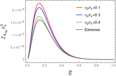
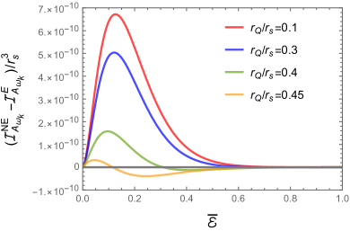
Figure 1: In left we have plotted the individual detector transition probabilities $\mathcal{I}_{A_{\omega_{k}}}$ of detector $A$ as a function of the dimensionless energy gap $\bar{\mathcal{E}}=r_{s}\,\Delta E$ in both the nonextremal and extremal scenarios. To obtain these plots we have fixed the dimensionless frequency of the field at $\bar{\omega}_{k}=r_{s}\,\omega_{k}=1$. In right we have plotted the difference between the nonextremal and extremal $\mathcal{I}_{A_{\omega_{k}}}$ as functions of $\bar{\mathcal{E}}$ for different $r_{Q}/r_{s}$. One observes that nonextremal detector transition is always greater than extremal, when $r_{Q}/r_{s}$ is low. However, near extremal limit $(r_{Q}/r_{s}\to 0.5)$, when $r_{Q}/r_{s}=0.4$ the nonextremal transition becomes lower compared to the extremal case for moderately large $\bar{\mathcal{E}}$. This feature is more prominent in $r_{Q}/r_{s}>0.4$ regime.

V.4 The measure of the harvested entanglement: concurrence

Here we detail our findings on the measure of the harvested entanglement, which is concurrence, in both the nonextremal and extremal scenarios. It is to be noted that for the static detector $B$ the integral $\mathcal{I}_{B_{\omega_{k}}}$ vanishes, which is evident from Eq. (V.1.1). Then the multiplication of $\mathcal{I}_{A_{\omega_{k}}}$ and $\mathcal{I}_{B_{\omega_{k}}}$ will also vanish, for all finite $\mathcal{I}_{A_{\omega_{k}}}$. From Eqs. (B.1) and (C.1) we observe for both the nonextremal and extremal cases that $\mathcal{I}_{A_{\omega_{k}}}$ are indeed finite. Then the concurrence is entirely given by $\mathcal{I}_{\varepsilon}$, see Eq. (9).

It is now convenient to define the concurrence to be $\bar{\mathcal{C}}_{\mathcal{I}}=|\bar{\mathcal{I}}^{W}_{\varepsilon}(\Delta E)+\bar{\mathcal{I}}^{R}_{\varepsilon}(\Delta E)|$. Let us also define some dimensionless parameters of the system, with respect to which we shall study the characteristics of the concurrence. We define the dimensionless parameters $\bar{\mathcal{E}}=r_{s}\,\Delta E$, $\bar{r}_{Q}=r_{Q}/r_{s}$, $\bar{d}_{n}=d_{n}/r_{s}$, $\bar{c}_{1}=c_{1}/r_{s}$, and $\bar{d}_{s}=d_{s}/r_{s}$. Then the extremal limit is given by $\bar{r}_{Q}\to 1/2$. With these considerations the dimensionless quantity that correspond to the concurrence is $\bar{\mathcal{C}}_{\mathcal{I}}/r_{s}^{3}$. In Fig. 2, 3, 4, 5, and 6 we have plotted this quantity with respect to different system parameters.

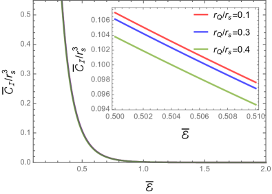
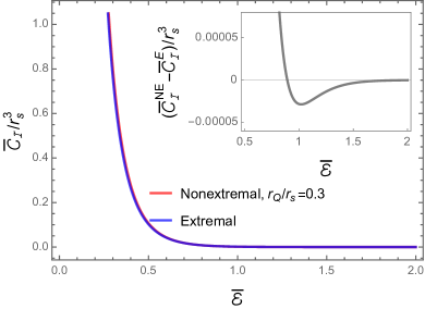
Figure 2: The concurrence in the nonextremal and extremal cases are plotted as functions of the dimensionless energy gap $\bar{\mathcal{E}}=r_{s}\,\Delta E$. In the left figure the concurrence in the nonextremal scenario is depicted. While in the right figure the same for both nonextremal and extremal scenarios are illustrated. To obtain these plots we have fixed the other parameters at $\bar{d}_{n}=d_{n}/r_{s}=0$, $\bar{c}_{1}=c_{1}/r_{s}=0$, and $\bar{d}_{s}=d_{s}/r_{s}=1$. In right plot for the nonextremal case we have fixed $\bar{r}_{Q}=r_{Q}/r_{s}=0.3$. From these plots it is evident that in both the nonextremal and extremal cases, harvesting decreases with increasing $\bar{\mathcal{E}}$. In the epilogue of the right plot we have also depicted the difference of the concurrences between the nonextremal and extremal scenarios in gray.

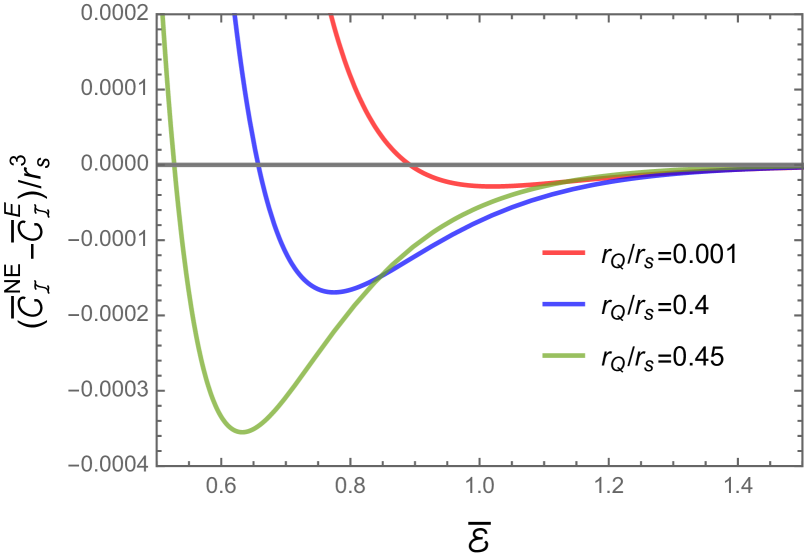
Figure 3: The difference in concurrences between the nonextremal and extremal scenarios is plotted as a functions of $\bar{\mathcal{E}}$ for different $\bar{r}_{Q}$. To obtain these plots we have fixed the other parameters at $\bar{d}_{n}=0$, $\bar{c}_{1}=0$, and $\bar{d}_{s}=1$. We find curves similar to that of $\bar{r}_{Q}=0.001$ for $\bar{r}_{Q}$ also many orders less than $0.001$. Therefore, in terms of concurrence, the difference between nonextremal and extremal scenarios broadly shows a specific feature for arbitrary $\bar{r}_{Q}$.

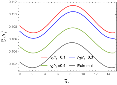
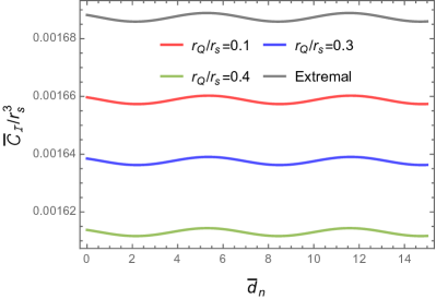
Figure 4: The concurrence in the nonextremal and extremal cases are plotted as functions of $\bar{d}_{n}$. To obtain these plots we have fixed the other parameters at $\bar{c}_{1}=0$ and $\bar{d}_{s}=1$. The left plot corresponds to $\bar{\mathcal{E}}=0.5$ and the right plot corresponds to $\bar{\mathcal{E}}=1$. With respect to the distance $\bar{d}_{n}$, that distinguishes different null paths, the concurrence in both cases are periodically dependant. In the left plot for $\bar{\mathcal{E}}=0.5$, the extremal curve has the lowest amplitude. While in the right plot for $\bar{\mathcal{E}}=1$, the extremal curve has the highest amplitude. This finding is consistent with our previous plots.

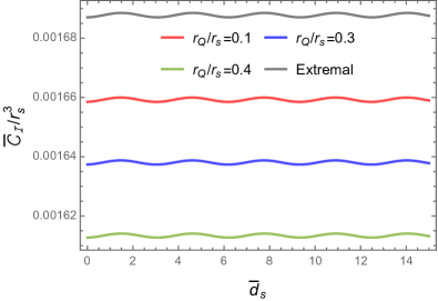
Figure 5: The concurrence in the nonextremal and extremal cases are plotted as functions of $\bar{d}_{s}$. To obtain these plots we have fixed the other parameters at $\bar{d}_{n}=0$ and $\bar{c}_{1}=0$. In the left plot we have fixed $\bar{\mathcal{E}}=0.5$ and in the right plot $\bar{\mathcal{E}}=1$. With respect to the radial distance $\bar{d}_{s}$ of the static detector $B$, the concurrence in both the nonextremal and the extremal cases are periodic, and qualitatively the same.

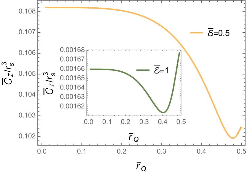
Figure 6: The concurrence in the nonextremal case is plotted as a function of $\bar{r}_{Q}=r_{Q}/r_{s}$. To obtain these plots we have fixed the other parameters at $\bar{d}_{n}=0$, $\bar{c}_{1}=0$, and $\bar{d}_{s}=1$. We fixed two different values of $\bar{\mathcal{E}}$ corresponding to two different curves.

For instance, in Fig. 2 we have plotted the concurrence as a function of the dimensionless detector energy gap $\bar{\mathcal{E}}$. In both the nonextremal (the left and right plots) and extremal (the right plot) cases the harvesting decreases with increasing $\bar{\mathcal{E}}$, and eventually becomes vanishing at large $\bar{\mathcal{E}}$. However the nonextremal and extremal plots are not exactly the same. From the epilogue of the right plot of Fig. 2 we observe that the nonextremal concurrence is larger than the extremal one at very low $\bar{\mathcal{E}}$. This gap decreases with increasing transition energy and becomes zero around $\bar{\mathcal{E}}\sim 0.8$, and then extremal concurrence becomes larger than the nonextremal one. Finally for very large $\bar{\mathcal{E}}\sim 1.5$ their difference is negligible and eventually the concurrences in both the cases become the same. Furthermore, in Fig. 3 we have plotted the difference between the nonextremal and extremal concurrences as a function of the energy gap $\bar{\mathcal{E}}$ for different $\bar{r}_{Q}$. Here from very low $\bar{r}_{Q}$ ($\bar{r}_{Q}=0.001$) to near extremal cases ($\bar{r}_{Q}=0.45$) one observes that this difference is positive in low $\bar{\mathcal{E}}$. While the harvesting is larger in the extremal case for moderately larger $\bar{\mathcal{E}}$. Therefore, unlike the single detector case in entanglement harvesting one perceives a persistent feature in the nonextremal and extremal cases for different black hole charges. This feature dictates that with very low detector transition energy one can harvest more entanglement from the nonextremal background. Whereas, with moderately large transition energy one is able to harvest maximum entanglement from the extremal background. It should be mentioned that, similar to the concurrence, in the single detector transition these features were not maintained thoroughly for arbitrary black hole charges, see the right plots of Fig. 1 and the discussion of V.3.

On the other hand, in Fig. 4 we have plotted the concurrence as a function of the dimensionless distance $\bar{d}_{n}$, that distinguishes different outgoing null paths. We observe that the harvesting is periodic with respect to this distance in both the nonextremal and the extremal scenarios. The periodicity and amplitude depend on the value of the detector transition energy $\bar{\mathcal{E}}$, as is perceived from the left and the right plots. At higher transition energy the amplitude is lower and the periodicity is greater. We also observe that for low detector transition energy $\bar{\mathcal{E}}=0.5$ (the left plot) the extremal case provides harvesting lower than the nonextremal case. While for high transition energy $\bar{\mathcal{E}}=1$ (the right plot) the extremal case provides more harvesting than the nonextremal one. This particular finding is also consistent with the prediction from the epilogue of the right plot of Fig. 2.

From Eqs. (V.1.2, V.1.2) of the nonextremal case and Eqs. (V.2.2, V.2.2) of the extremal case one can observe that there is an overall phase factor containing the parameter $\bar{c}_{1}$ in the integrals defining the concurrence. Now as the concurrence $\bar{\mathcal{C}}_{\mathcal{I}}$ is obtained from the modulus of these integrals, it will not depend on $\bar{c}_{1}$ . Therefore, in both the nonextremal and extremal cases the concurrence is independent of $\bar{c}_{1}$.

In Fig. (5) we have plotted the concurrence as a function of the dimensionless distance $\bar{d}_{s}$ of the static detector. For both the nonextremal and the extremal cases, the concurrence is found to be periodically dependent on $\bar{d}_{s}$, and qualitatively are the same. Here also the periodicity and amplitude of the concurrence depend on $\bar{\mathcal{E}}$, see the left and the right plots. For higher detector transition energy the periodicity is greater and the amplitude is lower. For low detector transition energy $\bar{\mathcal{E}}=0.5$ (the left plot) the extremal harvesting is lower than the nonextremal case. While for high transition energy $\bar{\mathcal{E}}=1$ (the right plot) the extremal harvesting is greater than the nonextremal one.

In Fig. 6 we plotted the concurrence in the nonextremal scenario as a function of the dimensionless charge $\bar{r}_{Q}$ of the black hole. The concurrence first decreases, and then increases with increasing $\bar{r}_{Q}$, as the charge $\bar{r}_{Q}\to 1/2$, i.e., the extremal limit. For $\bar{\mathcal{E}}=0.5$, the concurrence does not become greater than all the nonextremal harvesting in the extremal limit. On the other hand, for $\bar{\mathcal{E}}=1$, the concurrence in the extremal limit is seem to be always greater than the nonextremal case. This observation further solidifies our perception from the previous plots, that for large detector transition energy one may harvest more entanglement from the extremal background than the nonextremal case.

With these above observations one can obtain a perception on the quantitative distinction between the nonextremal and extremal Reissner-Nordström black hole backgrounds in terms of the harvested entanglement with one static Unruh-DeWitt detector and another one in outgoing null trajectory.

VI Quantification of “true harvesting”

In the previous section, we have estimated the concurrence, which gives a measure of the harvested entanglement. We observed that in the nonextremal and extremal scenarios with one static detector and another in outgoing null trajectory, the non-local terms $\mathcal{I}_{\varepsilon}$ solely contribute to the concurrence. While the local terms $\mathcal{I}_{j}$, arriving due to the static detectors vanish. Let us now identify specific characteristics of the harvested entanglement. In particular, how much of the concurrence depends on the background field state and how much does not. In this regard, one can express the Wightman functions of the non-local term $\mathcal{I}_{\varepsilon}$ as sums of expectations of field commutators and anti-commutators. The expectations of the field commutators are independent of the chosen field state, as they are proportional to the identity operator. Then the contributions from these commutators in the concurrence also cannot give any information about the background field state. One is asserted to assign this entanglement due to the communication between the detectors. In comparison, the contributions of anti-commutators in the concurrence are state-dependent. This contribution could be non-zero even if the detectors are causally disconnected; thus, the corresponding harvesting is called true harvesting Martin-Martinez (2015); Tjoa and Mann (2020); Gallock-Yoshimura et al. (2021); Tjoa and Martín-Martínez (2021). The idea of studying the anti-commutator and commutator in the $\mathcal{I}_{\varepsilon}$ term of concurrence to identify the true and communication-based harvesting was first introduced in Martin-Martinez (2015). Later this idea was also extensively used in Tjoa and Mann (2020); Gallock-Yoshimura et al. (2021); Tjoa and Martín-Martínez (2021); Barman et al. (2022d).

Let us now investigate the contributions in the concurrence due to true harvesting and communication channel, and also understand the features these quantities present in the nonextremal and extremal Reissner-Nordström black hole spacetime. In this regard, we express the integral $\mathcal{I}_{\varepsilon}$ from Eq. (II) as a sum of field commutator and anti-commutators

$$\mathcal{I}_{\varepsilon}=~{}-\mathcal{I}^{+}_{\varepsilon}-\mathcal{I}^{-}_{\varepsilon}~{},$$ (48)

where $\mathcal{I}^{+}_{\varepsilon}$ denotes the contribution from the vacuum expectations of the field anti-commutators, and $\mathcal{I}^{-}_{\varepsilon}$ correspond to field commutators. These integrals are given by

$$\mathcal{I}^{+}_{\varepsilon} = \int_{-\infty}^{\infty}d\tau_{B}\int_{-\infty}^{\infty}d\tau_{A}~{}\scalebox{0.91}{$e^{i(\Delta E^{B}\tau_{B}+\Delta E^{A}\tau_{A})}$}$$

$$\times\scalebox{0.87}{$\big{\{}G_{W}(X_{B},X_{A})+G_{W}(X_{A},X_{B})\big{\}}/2$}\,;$$ (49)

$$\mathcal{I}^{-}_{\varepsilon} = \int_{-\infty}^{\infty}d\tau_{B}\int_{-\infty}^{\infty}d\tau_{A}~{}\scalebox{0.91}{$e^{i(\Delta E^{B}\tau_{B}+\Delta E^{A}\tau_{A})}$}$$

$$\times \Big{[}\big{\{}G_{W}(X_{B},X_{A})-G_{W}(X_{A},X_{B})\big{\}}/2$$

$$+ \scalebox{0.87}{$\theta(T_{A}-T_{B})\left\{G_{W}\left(X_{A},X_{B}\right)-G_{W}\left(X_{B},X_{A}\right)\right\}\Big{]}$}.$$ (50)

We shall now study the contributions from $\mathcal{I}^{+}_{\varepsilon}$ and $\mathcal{I}^{-}_{\varepsilon}$ in both the nonextremal and extremal scenarios for different parameter values of the concerned spacetimes. We should also mention that one can define $\mathcal{I}^{+}_{\varepsilon_{\omega_{k}}}$ and $\mathcal{I}^{-}_{\varepsilon_{\omega_{k}}}$ corresponding to a certain field mode frequency $\omega_{k}$ as $\mathcal{I}^{\pm}_{\varepsilon}=\int_{0}^{\infty}d\omega_{k}\,\mathcal{I}^{\pm}_{\varepsilon_{\omega_{k}}}$. Then we will be evaluating these $\mathcal{I}^{\pm}_{\varepsilon_{\omega_{k}}}$ and study their absolute values, which seems adequate for our purpose to understand the true and communication based contributions in the entire harvesting. We mention that this particular proposal was initiated in Barman et al. (2022d).

VI.1 Nonextremal and extremal cases

In the previous section we have already evaluated the integrals $\mathcal{I}^{W}_{\varepsilon_{\omega_{k}}}$ and $\mathcal{I}^{R}_{\varepsilon_{\omega_{k}}}$ in the nonextremal and extremal scenarios. Then let us first try to express $\mathcal{I}^{\pm}_{\varepsilon_{\omega_{k}}}$ in terms of these previously evaluated quantities. In this regard, we first try to evaluate the part

$$\mathcal{I}^{W^{-}}_{\varepsilon} = \int_{-\infty}^{\infty}dt_{A}\int_{-\infty}^{\infty}dt_{B}~{}e^{i\Delta E(t_{B}+t_{A})}G_{W}(X_{A},X_{B})$$

$$= \int_{0}^{\infty}d\omega_{k}~{}\mathcal{I}^{W^{-}}_{\varepsilon_{\omega_{k}}}~{},$$ (51)

in Eqs. (49) and (50). This expression is true for both the nonextremal and extremal cases. Again in both the nonextremal and extremal scenarios, the integral $\mathcal{I}^{W^{-}}_{\varepsilon_{\omega_{k}}}$ can be expressed as

$$\mathcal{I}^{W^{-}}_{\varepsilon_{\omega_{k}}} = \frac{1}{4\pi\omega_{k}}\int_{-\infty}^{\infty}dt_{A}\int_{-\infty}^{\infty}dt_{B}~{}e^{i\Delta E(t_{B}+t_{A})}~{}$$

$$\times~{}\big{[}e^{-i\omega_{k}(u_{A}-u_{B})}+e^{-i\omega_{k}(v_{A}-v_{B})}\big{]}~{}$$

$$= \frac{e^{-i\omega_{k}\,(d_{n}-c_{1})}}{4\pi\omega_{k}}\,\int_{-\infty}^{\infty}dt_{A}\int_{-\infty}^{\infty}dt_{B}~{}e^{i\Delta E(t_{B}+t_{A})}~{}$$

$$\times~{}\big{[}e^{i\omega_{k}(t_{B}-d_{s})}+e^{-i\omega_{k}(2\,r_{\star_{A}}-t_{B}-d_{s})}\big{]}$$

$$= \frac{2\pi}{4\pi\omega_{k}}\,\delta(\omega_{k}+\Delta E)\,e^{-i\omega_{k}\,(d_{n}-c_{1})}\,\int_{-\infty}^{\infty}dt_{A}\,e^{i\Delta E\,t_{A}}~{}$$

$$\times~{}\big{[}e^{-i\omega_{k}\,d_{s}}+e^{-i\omega_{k}(2\,r_{\star_{A}}-d_{s})}\big{]}~{}.$$ (52)

We have considered $\Delta E>0$ and the integration over $\omega_{k}$ runs from zero to infinity. Naturally for the allowed range of $\omega_{k}$ the contribution from the Dirac delta $\delta(\omega_{k}+\Delta E)$ is always zero. Then the quantity $\mathcal{I}^{W^{-}}_{\varepsilon}$ with our considered set of detector trajectories, vanish in nonextremal and extremal Reissner-Nordström black hole spacetimes. Now defining $\mathcal{I}^{\pm}_{\varepsilon_{\omega_{k}}}=\delta(\omega_{k}-\Delta E)\,\bar{\mathcal{I}}^{\pm}_{\varepsilon}(\omega_{k})$ one can write

$$\bar{\mathcal{I}}^{+}_{\varepsilon}(\omega_{k}) = (1/2)\,\bar{\mathcal{I}}^{W}_{\varepsilon}(\omega_{k})~{},$$

$$\bar{\mathcal{I}}^{-}_{\varepsilon}(\omega_{k}) = (1/2)\,\bar{\mathcal{I}}^{W}_{\varepsilon}(\omega_{k})+\bar{\mathcal{I}}^{R}_{\varepsilon}(\omega_{k})~{};$$ (53)

where for nonextremal case one should use the expressions from Eq. (V.1.2) and (V.1.2). While for extremal case one should use the expressions from Eq. (V.2.2) and (V.2.2). We should note that while plotting these quantities $\bar{\mathcal{I}}^{\pm}_{\varepsilon}(\omega_{k})$, one should replace the $\omega_{k}$ with $\Delta E$, as only at $\omega_{k}=\Delta E$ the above quantities are non-vanishing.

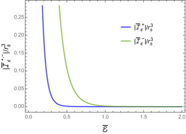
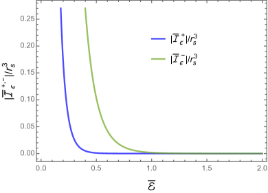
Figure 7: The contributions from the true and communication based harvesting in concurrence $|\bar{\mathcal{I}}^{\pm}_{\varepsilon}|$ are plotted in the nonextremal (left figure) and extremal (right figure) cases as functions of the dimensionless energy gap $\bar{\mathcal{E}}$. To obtain these plots we have fixed the other parameters at $\bar{r}_{Q}=0.3$, $\bar{d}_{n}=0$, $\bar{c}_{1}=0$, and $\bar{d}_{s}=1$. From these plots it is evident that in both the nonextremal and extremal cases harvesting from both sources decrease with increasing $\bar{\mathcal{E}}$. In all cases harvesting from the communication channel $|\bar{\mathcal{I}}^{-}_{\varepsilon}|$ is larger than the true harvesting $|\bar{\mathcal{I}}^{+}_{\varepsilon}|$

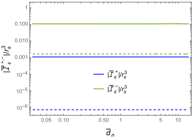
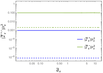
Figure 8: The contributions from the true and communication based harvesting in concurrence $|\bar{\mathcal{I}}^{\pm}_{\varepsilon}|$ are plotted in the nonextremal (left figure) and extremal (right figure) cases as functions of $\bar{d}_{n}$. To obtain these plots we have fixed the other parameters at $\bar{r}_{Q}=0.3$, $\bar{c}_{1}=0$, and $\bar{d}_{s}=1$. In both plots the solid lines correspond to $\bar{\mathcal{E}}=0.5$, and the dotted lines correspond to $\bar{\mathcal{E}}=1$.

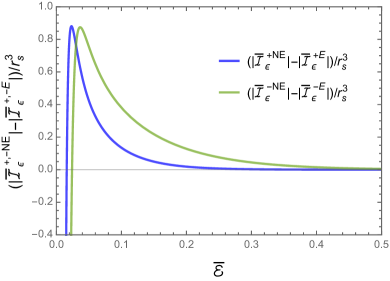
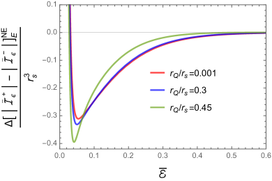
Figure 9: In left we have plotted the difference of the true and communication based harvesting between the nonextremal and extremal scenarios as a function of $\bar{\mathcal{E}}$. While in the right we have plotted the difference of $(|\bar{\mathcal{I}}^{+}_{\varepsilon}|-|\bar{\mathcal{I}}^{-}_{\varepsilon}|)$ from the nonextremal case to the extremal case. Here the expression of $\Delta[|\bar{\mathcal{I}}^{+}_{\varepsilon}|-|\bar{\mathcal{I}}^{-}_{\varepsilon}]^{NE}_{E}|$ is given by $(|\bar{\mathcal{I}}^{+{NE}}_{\varepsilon}|-|\bar{\mathcal{I}}^{-{NE}}_{\varepsilon}|)-(|\bar{\mathcal{I}}^{+{E}}_{\varepsilon}|-|\bar{\mathcal{I}}^{-{E}}_{\varepsilon}|)$. This quantity basically signifies a comparison of the dominance of the true harvesting over the communication based harvesting between the nonextremal and extremal scenarios. It is observed that in very low $\bar{\mathcal{E}}$ this dominance of true harvesting is higher in the nonextremal case. While in a bit higher $\bar{\mathcal{E}}$ this dominance is larger in the extremal case. We have fixed the other parameters at $\bar{d}_{n}=0$, $\bar{c}_{1}=0$, and $\bar{d}_{s}=1$. In the left plot we have fixed $\bar{r}_{Q}=0.3$.

In Fig. 7 we have plotted these $|\bar{\mathcal{I}}^{\pm}_{\varepsilon}(\Delta E)|$ as functions of the dimensionless energy $\bar{\mathcal{E}}$ in nonextremal (the left plot) and extremal (the right plot) scenarios respectively. From this figure one can observe that in both the nonextremal and extremal cases the harvesting only decreases with increasing $\bar{\mathcal{E}}$. Furthermore, in both the cases one perceives that the communication based harvesting ($|\bar{\mathcal{I}}^{-}_{\varepsilon}|$) is greater than the true harvesting ($|\bar{\mathcal{I}}^{+}_{\varepsilon}|$).

On the other hand, in Fig. 8 we have plotted $|\bar{\mathcal{I}}^{\pm}_{\varepsilon}(\Delta E)|$ as functions of the dimensionless distance $\bar{d}_{n}$ in the nonextremal (the left plot) and extremal (the right plot) scenarios. We found in both the cases that the true harvesting is lower than the communication based harvesting. Moreover, both the true and communication based harvesting decrease as the detector transition energy is increased.

As observed in the scenario of concurrence from the previous section here also the parameter $\bar{c}_{1}$ arrives in the integrals $|\bar{\mathcal{I}}^{\pm}_{\varepsilon}(\Delta E)|$ entirely inside a phase factor. Thus there is no contribution from this parameter in the modulus of these integrals. Moreover, we did not find any additional characteristics for the nonextremal and extremal scenarios in the plots of $|\bar{\mathcal{I}}^{\pm}_{\varepsilon}(\Delta E)|$ as a function of $\bar{d}_{s}$. Therefore, for the sake of brevity we have not included these plots. In the left side of Fig. 9 we have plotted the difference of $|\bar{\mathcal{I}}^{\pm}_{\varepsilon}(\Delta E)|$ between the nonextremal and extremal cases as a function of $\bar{\mathcal{E}}$. In the right side of Fig. 9 we have plotted defining a new quantity $(|\bar{\mathcal{I}}^{+}_{\varepsilon}|-|\bar{\mathcal{I}}^{-}_{\varepsilon}|)$, which signifies the dominance of the true harvesting over the communication based harvesting. The difference of this quantity between the nonextremal and extremal scenarios presents a feature similar to the total harvesting from the previous section. For example, this quantity is larger for nonextremal case when $\bar{\mathcal{E}}$ is very low. While this quantity is larger in the extremal scenario when $\bar{\mathcal{E}}$ is moderately greater.

VII Discussion

The concept of extremality is quite intriguing in a black hole spacetime. An extremal black hole does not Hawking radiate, though possessing an event horizon. Thus extremal black holes are qualitatively different from nonextremal ones. It is also suggested in the literature Ghosh and Mitra (1997); Gao (2003); Pradhan and Majumdar (2013) that to talk about the characteristics of an extremal black hole, one should start with an extremal one rather than taking the extremal limit of the nonextremal one. In this work, we have studied the characteristics of the entanglement harvesting profiles in nonextremal and extremal Reissner-Nordström black hole spacetimes. In this regard, we have considered detector $A$ in outgoing null trajectory and a static detector $B$. Our first observation is that the individual detector transition probability of detector $A$ corresponding to the Boulware like vacuum is non-vanishing in both nonextremal and extremal cases, see Fig. 1. We believe that the motion of the detector stimulates this nonzero transition probability also in the extremal case. In terms of this detector transition probability there is no specific feature in the difference between the nonextremal and the extremal scenarios for arbitrary black hole charge $r_{Q}$, see the right plots of Fig 1 and the discussion of subsection V.3. Furthermore, it will be interesting to construct suitable Kruskal-like coordinates in an extremal Reissner-Nordström black hole spacetime Gao (2003) and check the response of the static detector corresponding to the Unruh or Hartle-Hawking like vacuum. One should expect this detector response to be vanishing according to Hawking quanta’s vanishing number density in the extremal scenario. We are presently working in this direction and intend to present our findings in a future communication. Next, we observed that the individual detector transition probability vanishes for the static detector $B$, corresponding to the Boulware like vacuum.

On the other hand, in case of entanglement harvesting, we observed that it decreases with increasing detector transition energy for both the nonextremal and extremal black holes, see Fig. 2. Unlike the individual detector (for detector $A$) case, the difference in concurrence between the nonextremal and extremal scenarios exhibits a specific characteristic for arbitrary black hole charge $r_{Q}$. For example, this difference suggests one can harvest more entanglement from the nonextremal background than the extremal one, when the detector transition energy is very low. While for moderately large detector transition energy extremal case showcases maximum entanglement harvesting (Fig. 2, 3, 6). In Fig. 4 we observed that both the nonextremal and extremal harvesting is periodic with respect to the distance $d_{n}$ of the null paths of the detector $A$. Furthermore, from Fig. 5 a similar periodic nature is observed with respect to the distance $d_{s}$ of the static detector $B$. Our observations suggest these periodicities to be dependent on the detector transition energy. For instance, the periodicity increases with increasing transition energy. While the amplitude of this oscillation of concurrence decreases with elevating detector transition energy. Therefore, with our considered set-up and in terms of entanglement harvesting the nonextremal and extremal cases seem to be qualitatively indistinguishable. However, with different black hole parameters it is possible to tune the detector transition energy to understand the quantitative difference in the harvested entanglement.

Furthermore, while studying the origin of the harvested entanglement in Sec. VI we observed (Fig. 7 and Fig. 8) that the communication-based harvesting is larger in both the nonextremal and extremal scenarios. Both the communication based and true harvesting decreases with increasing detector transition energy. The qualitative nature of entanglement harvesting in the nonextremal and extremal scenarios are the same. Moreover, in this section we also defined the dominating true harvesting $(|\bar{\mathcal{I}}^{+}_{\varepsilon}|-|\bar{\mathcal{I}}^{-}_{\varepsilon}|)$, which denotes the dominance of true harvesting in comparison to the communication based harvesting. The difference of this quantity from the nonextremal to the extremal case shows a nature similar to the total harvesting with respect to the detector transition energy, see Fig. 9 and the discussion at the end of VI.1.

Finally, we shall like to mention (we observed it, though not included in the manuscript) that two static detectors do not harvest any entanglement from the Boulware like vacuum of the Reissner-Nordström black hole background. A similar phenomenon is also observed in Gallock-Yoshimura et al. (2021) in the Schwarzschild background. Moreover, one may also consider both of the detectors to be in null trajectories like done in Barman et al. (2022d). But in that case, evaluating the non-local entangling term becomes a challenge analytically. We like to pursue these issues in future.

Appendix A Nonextremal tortoise coordinate in the limit $r_{Q}\to r_{s}/2$

In order to realize the limit $r_{Q}\to r_{s}/2$ of the tortoise coordinate in Eq. (13) of the nonextremal case and thus to get the extremal expression (14), we consider $r_{s}^{2}-4r_{Q}^{2}=r_{s}^{2}\,\varsigma^{2}$. Then $\varsigma\to 0$ should represent the extremal scenario. With this consideration one has $r_{\pm}=(1\pm\varsigma)\,r_{s}/2$ and $\kappa_{\pm}=2\varsigma/[r_{s}(1\pm\varsigma)^{2}]$. Then around $\varsigma=0$ one can approximate the quantity

$$\ln\Big{(}\frac{r}{r_{\pm}}-1\Big{)} = \ln\Big{(}\frac{2r}{r_{s}(1\pm\varsigma)}-1\Big{)}$$

$$\approx \ln\Big{(}\frac{2r}{r_{s}}(1\mp\varsigma)-1\Big{)}$$

$$= \ln\Big{(}\frac{2r}{r_{s}}-1\Big{)}+\ln\Big{(}1\mp\frac{2r\varsigma}{2r-r_{s}}\Big{)}$$

$$\approx \ln\Big{(}\frac{2r}{r_{s}}-1\Big{)}\mp\frac{2r\varsigma}{2r-r_{s}}~{}.$$ (54)

It should be noted that in the last expression we have used the approximation $\ln(1\mp\delta)\approx\mp\delta$, for very small positive $\delta$. Now one may use the previous expression in (13) to get

$$r_{\star} \approx r+\frac{r_{s}\varsigma}{\varsigma}\ln\Big{(}\frac{2r}{r_{s}}-1\Big{)}-\frac{rr_{s}(1+\varsigma^{2})}{2r-r_{s}}$$

$$= r+r_{s}\ln\Big{(}\frac{2r}{r_{s}}-1\Big{)}-\frac{(r_{s}^{2}/4)(1+\varsigma^{2})}{r-r_{s}/2}-\frac{r_{s}(1+\varsigma^{2})}{2}~{}.$$

In the limit of $\varsigma\to 0$ this expression looks same as the extremal expression of the tortoise coordinate (14) up-to a constant additive quantity $(-r_{s}/2)$. One should notice that due to the presence of both the $(1/2\kappa_{\pm})\,\ln(r/r_{\pm}-1)$ terms in the expression of the nonextremal tortoise coordinate (13), there was this appearance of zero divided by zero in the extremal limit. This zero by zero form is evident from the first expression of Eq. (A), which does not create too much hurdle to get the extremal expression (14) eventually. However, one should note that during further calculations of $\mathcal{I}_{j}$ and $\mathcal{I}_{\varepsilon}$ when the terms $(1/2\kappa_{\pm})\,\ln(r/r_{\pm}-1)$ are not kept together the limit to extremality may not occur as easily. Therefore, it seems necessary to consider the nonextremal and extremal scenarios separately from the beginning to estimate the integrals $\mathcal{I}_{j}$ and $\mathcal{I}_{\varepsilon}$.

Appendix B Evaluation of $\mathcal{I}_{j}$ and $\mathcal{I}_{\varepsilon}$ in nonextremal Reissner-Nordström spacetime

B.1 Evaluation of $\mathcal{I}_{A_{\omega_{k}}}$

In Eq. (V.1.1) let us consider that $\mathcal{I}_{A_{\omega_{k}}}=(r_{+}^{2}/4\pi\omega_{k})\,|\bar{\mathcal{I}}_{A_{\omega_{k}}}|^{2}$. The integral $\bar{\mathcal{I}}_{A_{\omega_{k}}}$ can be evaluated analytically introducing a regulator of the form $e^{-\epsilon\,y_{A}}y_{A}^{\epsilon}$, with small positive and real $\epsilon$. The integrated out expression is

$$\bar{\mathcal{I}}_{A_{\omega_{k}}} = -2\pi e^{\frac{\pi(\Delta E+\omega_{k}-i\kappa_{+}\epsilon)}{\kappa_{+}}}\left(\tfrac{r_{+}}{r_{-}}-1\right)^{-\frac{i(\Delta E+\omega_{k})}{\kappa_{-}}}r_{+}^{-\epsilon-\frac{i(\Delta E+\omega_{k})}{\kappa_{+}}}(r_{-}-r_{+})^{\epsilon+\frac{i(\Delta E+\omega_{k})}{\kappa_{+}}}\text{csch}\left(-\tfrac{\pi(\Delta E+\omega_{k})}{\kappa_{+}}+\tfrac{\pi(\Delta E+\omega_{k}+i\kappa_{-}\epsilon)}{\kappa_{-}}\right)$$

$$\times~{}\Bigg{[}\tfrac{1}{r_{+}-r_{-}}\tfrac{1}{{r_{+}(\Delta E+\omega_{k})(\epsilon-ir_{+}(\Delta E+2\omega_{k}))\Gamma\left(\frac{i(\omega_{k}+\Delta E)}{\kappa_{-}}\right)}}$$

$$\times~{}\Bigg{\{}\Gamma\left(\tfrac{i(\omega_{k}+\Delta E)}{\kappa_{+}}+\epsilon\right)\Bigg{(}i\left(r_{+}(r_{-}-r_{+})(\Delta E+\omega_{k})+\kappa_{-}r_{-}^{2}(r_{+}(\Delta E+2\omega_{k})+i\epsilon)\right)\,$$

$$\times~{}_{1}\tilde{F}_{1}\left(\tfrac{i(\omega_{k}+\Delta E)}{\kappa_{+}}+\epsilon;\epsilon+\tfrac{i(\omega_{k}+\Delta E)(\kappa_{-}-\kappa_{+})}{\kappa_{-}\kappa_{+}};\tfrac{i(r_{-}-r_{+})(r_{+}(2\omega_{k}+\Delta E)+i\epsilon)}{r_{+}}\right)$$

$$-~{}\frac{1}{\kappa_{-}\kappa_{+}}\bigg{(}(r_{-}-r_{+})(\Delta E+\omega_{k})(-\kappa_{-}r_{+}(\Delta E+\omega_{k})$$

$$+~{}\kappa_{+}(\kappa_{-}r_{+}(r_{-}+r_{+})(\Delta E+2\omega_{k})+i\kappa_{-}\epsilon(r_{-}+2r_{+})+r_{+}(\Delta E+\omega_{k})))\,$$

$$\times~{}_{1}\tilde{F}_{1}\left(\tfrac{i(\omega_{k}+\Delta E)}{\kappa_{+}}+\epsilon;\epsilon+\tfrac{i(\omega_{k}+\Delta E)(\kappa_{-}-\kappa_{+})}{\kappa_{-}\kappa_{+}}+1;\tfrac{i(r_{-}-r_{+})(r_{+}(2\omega_{k}+\Delta E)+i\epsilon)}{r_{+}}\right)\bigg{)}\Bigg{)}\Bigg{\}}$$

$$-~{}(\epsilon-ir_{+}(\Delta E+2\omega_{k}))^{-\epsilon-\frac{i(\kappa_{-}-\kappa_{+})(\Delta E+\omega_{k})}{\kappa_{-}\kappa_{+}}}\left(1-\tfrac{r_{-}}{r_{+}}\right)^{-\epsilon-\frac{i(\kappa_{-}-\kappa_{+})(\Delta E+\omega_{k})}{\kappa_{-}\kappa_{+}}}$$

$$\times~{}\Bigg{\{}2i\,_{1}\tilde{F}_{1}\left(\tfrac{i(\omega_{k}+\Delta E)}{\kappa_{-}}+1;-\epsilon-\tfrac{i(\omega_{k}+\Delta E)(\kappa_{-}-\kappa_{+})}{\kappa_{-}\kappa_{+}}+1;\tfrac{i(r_{-}-r_{+})(r_{+}(2\omega_{k}+\Delta E)+i\epsilon)}{r_{+}}\right)$$

$$-~{}(r_{+}(\Delta E+2\omega_{k})+i\epsilon)\,_{1}\tilde{F}_{1}\left(\tfrac{i(\omega_{k}+\Delta E)}{\kappa_{-}}+1;-\epsilon-\tfrac{i(\omega_{k}+\Delta E)(\kappa_{-}-\kappa_{+})}{\kappa_{-}\kappa_{+}}+2;\tfrac{i(r_{-}-r_{+})(r_{+}(2\omega_{k}+\Delta E)+i\epsilon)}{r_{+}}\right)\Bigg{\}}$$

$$+~{}i(\epsilon-ir_{+}(\Delta E+2\omega_{k}))^{-\frac{i(\kappa_{-}-\kappa_{+})(\Delta E+\omega_{k})}{\kappa_{-}\kappa_{+}}-\epsilon-1}\left(1-\tfrac{r_{-}}{r_{+}}\right)^{-\epsilon-\frac{i(\kappa_{-}-\kappa_{+})(\Delta E+\omega_{k})}{\kappa_{-}\kappa_{+}}}\,$$

$$\times~{}_{1}\tilde{F}_{1}\left(\tfrac{i(\omega_{k}+\Delta E)}{\kappa_{-}}+1;i\left(\tfrac{\omega_{k}+\Delta E+i\epsilon\kappa_{-}}{\kappa_{-}}-\tfrac{\omega_{k}+\Delta E}{\kappa_{+}}\right);\tfrac{i(r_{-}-r_{+})(r_{+}(2\omega_{k}+\Delta E)+i\epsilon)}{r_{+}}\right)\Bigg{]}~{}.$$ (56)

B.2 Evaluation of $\mathcal{I}_{\varepsilon_{\omega_{k}}}$

First, introducing regulators of the form $e^{-\epsilon\,y_{A}}y_{A}^{\epsilon}$, one can evaluate $\bar{\mathcal{I}}^{W}_{\varepsilon}(\omega_{k})$ as

$$\bar{\mathcal{I}}^{W}_{\varepsilon}(\omega_{k}) = \frac{r_{+}^{2}r_{s}}{\omega_{k}}\,~{}\frac{e^{i\omega_{k}\,(d_{n}-c_{1}-d_{s})}\,e^{i\Delta E\,d_{n}}}{4\kappa_{-}^{2}\kappa_{+}^{2}}ie^{ir_{+}(2\omega_{k}+\Delta E)}(r_{-}-r_{+})^{\frac{i(\omega_{k}+\Delta E-i\epsilon\kappa_{+})}{\kappa_{+}}}r_{+}^{-\frac{i(\omega_{k}+\Delta E-i(\epsilon+4)\kappa_{+})}{\kappa_{+}}}\left(\tfrac{r_{+}}{r_{-}}-1\right)^{-\frac{i(\omega_{k}+\Delta E)}{\kappa_{-}}}$$

$$\times~{}\Bigg{[}\tfrac{1}{r_{+}(2\omega_{k}+\Delta E)+i\epsilon}\Bigg{\{}4\left(1-\tfrac{r_{-}}{r_{+}}\right)^{-\frac{i(\omega_{k}(\kappa_{-}-\kappa_{+})+\Delta E(\kappa_{-}-\kappa_{+})-i\epsilon\kappa_{-}\kappa_{+})}{\kappa_{-}\kappa_{+}}}$$

$$\times~{}r_{+}^{3}(\epsilon-ir_{+}(2\omega_{k}+\Delta E))^{-\frac{i(\omega_{k}(\kappa_{-}-\kappa_{+})+\Delta E(\kappa_{-}-\kappa_{+})-i\epsilon\kappa_{-}\kappa_{+})}{\kappa_{-}\kappa_{+}}}\Gamma\left(\tfrac{i\omega_{k}(\kappa_{-}-\kappa_{+})+i\Delta E(\kappa_{-}-\kappa_{+})+(\epsilon-1)\kappa_{-}\kappa_{+}}{\kappa_{-}\kappa_{+}}\right)$$

$$\times~{}\Bigg{(}-e^{\frac{\pi(\omega_{k}+\Delta E-i(\epsilon-2)\kappa_{+})}{\kappa_{+}}}(r_{+}(2\omega_{k}+\Delta E)+i\epsilon)^{2}\kappa_{-}^{2}\,$$

$$\times~{}_{1}F_{1}\left(\tfrac{i\omega_{k}+i\Delta E+\kappa_{-}}{\kappa_{-}};-\tfrac{i(\omega_{k}(\kappa_{-}-\kappa_{+})+\Delta E(\kappa_{-}-\kappa_{+})-i(\epsilon-2)\kappa_{-}\kappa_{+})}{\kappa_{-}\kappa_{+}};\tfrac{(r_{+}-r_{-})(\epsilon-ir_{+}(2\omega_{k}+\Delta E))}{r_{+}}\right)\kappa_{+}^{2}$$

$$+~{}2e^{\frac{\pi(\omega_{k}+\Delta E-i(\epsilon-1)\kappa_{+})}{\kappa_{+}}}(r_{+}(2\omega_{k}+\Delta E)+i\epsilon)\kappa_{-}(i(\epsilon-1)\kappa_{-}\kappa_{+}+\omega_{k}(\kappa_{+}-\kappa_{-})+\Delta E(\kappa_{+}-\kappa_{-}))\,$$

$$\times~{}_{1}F_{1}\left(\tfrac{i\omega_{k}+i\Delta E+\kappa_{-}}{\kappa_{-}};-\tfrac{i(\omega_{k}(\kappa_{-}-\kappa_{+})+\Delta E(\kappa_{-}-\kappa_{+})-i(\epsilon-1)\kappa_{-}\kappa_{+})}{\kappa_{-}\kappa_{+}};\tfrac{(r_{+}-r_{-})(\epsilon-ir_{+}(2\omega_{k}+\Delta E))}{r_{+}}\right)\kappa_{+}$$

$$-~{}e^{\frac{\pi(\omega_{k}+\Delta E-i\epsilon\kappa_{+})}{\kappa_{+}}}(i(\epsilon-1)\kappa_{-}\kappa_{+}+\omega_{k}(\kappa_{+}-\kappa_{-})+\Delta E(\kappa_{+}-\kappa_{-}))(i\epsilon\kappa_{-}\kappa_{+}+\omega_{k}(\kappa_{+}-\kappa_{-})+\Delta E(\kappa_{+}-\kappa_{-}))\,$$

$$\times~{}_{1}F_{1}\left(\tfrac{i\omega_{k}+i\Delta E+\kappa_{-}}{\kappa_{-}};-\tfrac{i(\omega_{k}(\kappa_{-}-\kappa_{+})+\Delta E(\kappa_{-}-\kappa_{+})-i\epsilon\kappa_{-}\kappa_{+})}{\kappa_{-}\kappa_{+}};\tfrac{(r_{+}-r_{-})(\epsilon-ir_{+}(2\omega_{k}+\Delta E))}{r_{+}}\right)\Bigg{)}\Bigg{\}}$$

$$+~{}\tfrac{1}{(r_{-}-r_{+})(\omega_{k}+\Delta E)\Gamma\left(\frac{i(\omega_{k}+\Delta E)}{\kappa_{-}}\right)}\Bigg{\{}\kappa_{-}\Gamma\left(\tfrac{i(\omega_{k}+\Delta E-i\epsilon\kappa_{+})}{\kappa_{+}}\right)\Gamma\left(-\tfrac{i(\omega_{k}(\kappa_{-}-\kappa_{+})+\Delta E(\kappa_{-}-\kappa_{+})-i(\epsilon+1)\kappa_{-}\kappa_{+})}{\kappa_{-}\kappa_{+}}\right)$$

$$\times~{}\Bigg{(}-4e^{\frac{\pi(\omega_{k}+\Delta E-i(\epsilon-2)\kappa_{+})}{\kappa_{+}}}(i\epsilon\kappa_{-}\kappa_{+}+\omega_{k}(\kappa_{+}-\kappa_{-})+\Delta E(\kappa_{+}-\kappa_{-}))$$

$$\times~{}(i(\epsilon+1)\kappa_{-}\kappa_{+}+\omega_{k}(\kappa_{+}-\kappa_{-})+\Delta E(\kappa_{+}-\kappa_{-}))\,$$

$$\times~{}_{1}F_{1}\left(\tfrac{i(\omega_{k}+\Delta E-i\epsilon\kappa_{+})}{\kappa_{+}};\tfrac{i\omega_{k}(\kappa_{-}-\kappa_{+})+i\Delta E(\kappa_{-}-\kappa_{+})+\epsilon\kappa_{-}\kappa_{+}}{\kappa_{-}\kappa_{+}};\frac{(r_{+}-r_{-})(\epsilon-ir_{+}(2\omega_{k}+\Delta E))}{r_{+}}\right)r_{+}^{4}$$

$$+~{}8e^{\frac{\pi(\omega_{k}+\Delta E-i(\epsilon-1)\kappa_{+})}{\kappa_{+}}}(r_{+}-r_{-})\kappa_{-}(\omega_{k}+\Delta E-i\epsilon\kappa_{+})(i(\epsilon+1)\kappa_{-}\kappa_{+}+\omega_{k}(\kappa_{+}-\kappa_{-})+\Delta E(\kappa_{+}-\kappa_{-}))\,$$

$$\times~{}_{1}F_{1}\left(\tfrac{i\omega_{k}+i\Delta E+\epsilon\kappa_{+}+\kappa_{+}}{\kappa_{+}};\tfrac{i\omega_{k}(\kappa_{-}-\kappa_{+})+i\Delta E(\kappa_{-}-\kappa_{+})+(\epsilon+1)\kappa_{-}\kappa_{+}}{\kappa_{-}\kappa_{+}};\tfrac{(r_{+}-r_{-})(\epsilon-ir_{+}(2\omega_{k}+\Delta E))}{r_{+}}\right)r_{+}^{3}$$

$$-~{}4e^{\frac{\pi(\omega_{k}+\Delta E-i\epsilon\kappa_{+})}{\kappa_{+}}}(r_{-}-r_{+})^{2}\kappa_{-}^{2}(\omega_{k}+\Delta E-i\epsilon\kappa_{+})(\omega_{k}+\Delta E-i(\epsilon+1)\kappa_{+})\,$$

$$\times~{}_{1}F_{1}\left(\tfrac{i\omega_{k}+i\Delta E+(\epsilon+2)\kappa_{+}}{\kappa_{+}};\tfrac{i\omega_{k}(\kappa_{-}-\kappa_{+})+i\Delta E(\kappa_{-}-\kappa_{+})+(\epsilon+2)\kappa_{-}\kappa_{+}}{\kappa_{-}\kappa_{+}};\tfrac{(r_{+}-r_{-})(\epsilon-ir_{+}(2\omega_{k}+\Delta E))}{r_{+}}\right)r_{+}^{2}\Bigg{)}\Bigg{\}}\Bigg{]}~{}.$$ (57)

Second, introducing regulators of the form $e^{-\epsilon\,y_{A}}y_{A}^{\epsilon}$, one can evaluate the integral $\bar{\mathcal{I}}^{R}_{\varepsilon}(\omega_{k})$ with the first part in the braces in Eq. (V.1.2). Let us call this part $\bar{\mathcal{I}}^{R^{+}}_{\varepsilon}(\omega_{k})$, which can be evaluated as

$$\bar{\mathcal{I}}^{R^{+}}_{\varepsilon}(\omega_{k}) = -\frac{r_{+}^{2}r_{s}\,e^{i\Delta E(d_{n}-c_{1})}}{2\,\omega_{k}}~{}\times\frac{1}{4}e^{i(d_{s}\omega_{k}-r_{+}\omega_{k}+2r_{+}\Delta E)}\left(\frac{r_{+}}{r_{-}}-1\right)^{\frac{i(\omega_{k}-3\Delta E)}{2\kappa_{-}}}$$

$$\times~{}\Bigg{[}i\left(1-\frac{r_{-}}{r_{+}}\right)^{\frac{i(-3\Delta E\kappa_{-}+2i\epsilon\kappa_{+}\kappa_{-}+\omega_{k}(\kappa_{-}-\kappa_{+})+3\Delta E\kappa_{+})}{2\kappa_{-}\kappa_{+}}}(r_{-}-r_{+})^{-\frac{i(\omega_{k}-3\Delta E+2i\epsilon\kappa_{+})}{2\kappa_{+}}}$$

$$\times~{}(ir_{+}(\omega_{k}-2\Delta E)+\epsilon)^{\frac{i(-3\Delta E\kappa_{-}+2i\epsilon\kappa_{+}\kappa_{-}+\omega_{k}(\kappa_{-}-\kappa_{+})+3\Delta E\kappa_{+})}{2\kappa_{-}\kappa_{+}}}\Gamma\left(\tfrac{-i\omega_{k}(\kappa_{-}-\kappa_{+})+3i\Delta E(\kappa_{-}-\kappa_{+})+2(\epsilon-1)\kappa_{-}\kappa_{+}}{2\kappa_{-}\kappa_{+}}\right)$$

$$\times~{}\Bigg{\{}4e^{-\frac{\pi(\omega_{k}-3\Delta E+2i(\epsilon-2)\kappa_{+})}{2\kappa_{+}}}(r_{+}(\omega_{k}-2\Delta E)-i\epsilon)\,$$

$$\times~{}_{1}F_{1}\left(-\tfrac{i(\omega_{k}-3\Delta E+2i\kappa_{-})}{2\kappa_{-}};\tfrac{i(\omega_{k}(\kappa_{-}-\kappa_{+})-3\Delta E(\kappa_{-}-\kappa_{+})+2i(\epsilon-2)\kappa_{-}\kappa_{+})}{2\kappa_{-}\kappa_{+}};\tfrac{(r_{+}-r_{-})(ir_{+}(\omega_{k}-2\Delta E)+\epsilon)}{r_{+}}\right)$$

$$+~{}\frac{1}{\kappa_{-}\kappa_{+}}\Bigg{(}4e^{-\frac{\pi(\omega_{k}-3\Delta E+2i(\epsilon-1)\kappa_{+})}{2\kappa_{+}}}(\omega_{k}(\kappa_{-}-\kappa_{+})-3\Delta E(\kappa_{-}-\kappa_{+})+2i(\epsilon-1)\kappa_{-}\kappa_{+})\,$$

$$\times~{}_{1}F_{1}\left(-\tfrac{i(\omega_{k}-3\Delta E+2i\kappa_{-})}{2\kappa_{-}};\tfrac{i(\omega_{k}(\kappa_{-}-\kappa_{+})-3\Delta E(\kappa_{-}-\kappa_{+})+2i(\epsilon-1)\kappa_{-}\kappa_{+})}{2\kappa_{-}\kappa_{+}};\tfrac{(r_{+}-r_{-})(ir_{+}(\omega_{k}-2\Delta E)+\epsilon)}{r_{+}}\right)\Bigg{)}$$

$$-~{}\frac{1}{(-r_{+}\omega_{k}+2r_{+}\Delta E+i\epsilon)\kappa_{-}^{2}\kappa_{+}^{2}}\Bigg{(}e^{-\frac{\pi(\omega_{k}-3\Delta E+2i\epsilon\kappa_{+})}{2\kappa_{+}}}(\omega_{k}(\kappa_{-}-\kappa_{+})-3\Delta E(\kappa_{-}-\kappa_{+})$$

$$+~{}2i(\epsilon-1)\kappa_{-}\kappa_{+})(-3\Delta E\kappa_{-}+2i\epsilon\kappa_{+}\kappa_{-}+\omega_{k}(\kappa_{-}-\kappa_{+})+3\Delta E\kappa_{+})\,$$

$$\times~{}_{1}F_{1}\left(-\tfrac{i(\omega_{k}-3\Delta E+2i\kappa_{-})}{2\kappa_{-}};\tfrac{i(-3\Delta E\kappa_{-}+2i\epsilon\kappa_{+}\kappa_{-}+\omega_{k}(\kappa_{-}-\kappa_{+})+3\Delta E\kappa_{+})}{2\kappa_{-}\kappa_{+}};\tfrac{(r_{+}-r_{-})(ir_{+}(\omega_{k}-2\Delta E)+\epsilon)}{r_{+}}\right)\Bigg{)}\Bigg{\}}$$

$$\times r_{+}^{\frac{i(\omega_{k}-3\Delta E+2i(\epsilon+1)\kappa_{+})}{2\kappa_{+}}}+\frac{1}{\kappa_{+}^{2}\Gamma\left(-\frac{i(\omega_{k}-3\Delta E+2i\kappa_{-})}{2\kappa_{-}}\right)}\Bigg{\{}\left(\tfrac{r_{-}}{r_{+}}-1\right)^{-\frac{i(\omega_{k}-3\Delta E+2i\epsilon\kappa_{+})}{2\kappa_{+}}}\Gamma\left(-\tfrac{i(\omega_{k}-3\Delta E+2i\epsilon\kappa_{+})}{2\kappa_{+}}\right)$$

$$\times~{}\Gamma\left(\tfrac{i(\omega_{k}(\kappa_{-}-\kappa_{+})-3\Delta E(\kappa_{-}-\kappa_{+})+2i(\epsilon+1)\kappa_{-}\kappa_{+})}{2\kappa_{-}\kappa_{+}}\right)\Bigg{(}\frac{1}{(r_{-}-r_{+})\kappa_{-}^{2}}\bigg{(}e^{-\frac{\pi(\omega_{k}-3\Delta E+2i(\epsilon-2)\kappa_{+})}{2\kappa_{+}}}$$

$$\times~{}(-3\Delta E\kappa_{-}+2i\epsilon\kappa_{+}\kappa_{-}+\omega_{k}(\kappa_{-}-\kappa_{+})+3\Delta E\kappa_{+})(\omega_{k}(\kappa_{-}-\kappa_{+})-3\Delta E(\kappa_{-}-\kappa_{+})+2i(\epsilon+1)\kappa_{-}\kappa_{+})\,$$

$$\times~{}_{1}F_{1}\left(-\tfrac{i(\omega_{k}-3\Delta E+2i\epsilon\kappa_{+})}{2\kappa_{+}};-\tfrac{i(-3\Delta E\kappa_{-}+2i\epsilon\kappa_{+}\kappa_{-}+\omega_{k}(\kappa_{-}-\kappa_{+})+3\Delta E\kappa_{+})}{2\kappa_{-}\kappa_{+}};\tfrac{(r_{+}-r_{-})(ir_{+}(\omega_{k}-2\Delta E)+\epsilon)}{r_{+}}\right)\bigg{)}$$

$$+~{}\frac{1}{r_{+}\kappa_{-}}\bigg{(}2e^{-\frac{\pi(\omega_{k}-3\Delta E+2i(\epsilon-1)\kappa_{+})}{2\kappa_{+}}}(\omega_{k}-3\Delta E+2i\epsilon\kappa_{+})(3\Delta E(\kappa_{-}-\kappa_{+})-2i(\epsilon+1)\kappa_{-}\kappa_{+}+\omega_{k}(\kappa_{+}-\kappa_{-}))\,$$

$$\times~{}_{1}F_{1}\left(\epsilon-\tfrac{i(\omega_{k}-3\Delta E+2i\kappa_{+})}{2\kappa_{+}};\tfrac{-i\omega_{k}(\kappa_{-}-\kappa_{+})+3i\Delta E(\kappa_{-}-\kappa_{+})+2(\epsilon+1)\kappa_{-}\kappa_{+}}{2\kappa_{-}\kappa_{+}};\tfrac{(r_{+}-r_{-})(ir_{+}(\omega_{k}-2\Delta E)+\epsilon)}{r_{+}}\right)\bigg{)}$$

$$+~{}\frac{1}{r_{+}^{2}}\bigg{(}e^{-\frac{\pi(\omega_{k}-3\Delta E+2i\epsilon\kappa_{+})}{2\kappa_{+}}}(r_{-}-r_{+})(\omega_{k}-3\Delta E+2i\epsilon\kappa_{+})(\omega_{k}-3\Delta E+2i(\epsilon+1)\kappa_{+})\,$$

$$\times~{}_{1}F_{1}\left(\epsilon-\tfrac{i(\omega_{k}-3\Delta E+4i\kappa_{+})}{2\kappa_{+}};\tfrac{-i\omega_{k}(\kappa_{-}-\kappa_{+})+3i\Delta E(\kappa_{-}-\kappa_{+})+2(\epsilon+2)\kappa_{-}\kappa_{+}}{2\kappa_{-}\kappa_{+}};\tfrac{(r_{+}-r_{-})(ir_{+}(\omega_{k}-2\Delta E)+\epsilon)}{r_{+}}\right)\bigg{)}\Bigg{)}\Bigg{\}}\Bigg{]}~{}.$$ (58)

Similarly one can evaluate the second part of $\bar{\mathcal{I}}^{R}_{\varepsilon}(\omega_{k})$ in the braces in Eq. (V.1.2). We call that part to be $\bar{\mathcal{I}}^{R^{-}}_{\varepsilon}(\omega_{k})$ and is expressed as

$$\bar{\mathcal{I}}^{R^{-}}_{\varepsilon}(\omega_{k}) = -\frac{r_{+}^{2}r_{s}\,e^{i\Delta E(d_{n}-c_{1})}}{2\,\omega_{k}}~{}\times\frac{1}{4\kappa_{-}^{2}\kappa_{+}^{2}}\Bigg{[}e^{ir_{+}(\omega_{k}+2\Delta E)-id_{s}\omega_{k}}\left(\frac{r_{+}}{r_{-}}-1\right)^{-\frac{i(\omega_{k}+3\Delta E)}{2\kappa_{-}}}\Bigg{\{}\frac{1}{r_{+}(\omega_{k}+2\Delta E)+i\epsilon}$$

$$\times~{}\Bigg{(}i\left(1-\frac{r_{-}}{r_{+}}\right)^{-\frac{i(\omega_{k}(\kappa_{-}-\kappa_{+})+3\Delta E(\kappa_{-}-\kappa_{+})-2i\epsilon\kappa_{-}\kappa_{+})}{2\kappa_{-}\kappa_{+}}}(r_{-}-r_{+})^{\frac{i(\omega_{k}+3\Delta E-2i\epsilon\kappa_{+})}{2\kappa_{+}}}r_{+}^{-\frac{i\omega_{k}+3i\Delta E+2(\epsilon+1)\kappa_{+}}{2\kappa_{+}}}$$

$$\times~{}(\epsilon-ir_{+}(\omega_{k}+2\Delta E))^{-\frac{i(\omega_{k}(\kappa_{-}-\kappa_{+})+3\Delta E(\kappa_{-}-\kappa_{+})-2i\epsilon\kappa_{-}\kappa_{+})}{2\kappa_{-}\kappa_{+}}}\Gamma\left(\tfrac{i\omega_{k}(\kappa_{-}-\kappa_{+})+3i\Delta E(\kappa_{-}-\kappa_{+})+2(\epsilon-1)\kappa_{-}\kappa_{+}}{2\kappa_{-}\kappa_{+}}\right)$$

$$\times~{}\bigg{(}-4e^{\frac{\pi(\omega_{k}+3\Delta E-2i(\epsilon-2)\kappa_{+})}{2\kappa_{+}}}(r_{+}(\omega_{k}+2\Delta E)+i\epsilon)^{2}\kappa_{-}^{2}\,$$

$$\times~{}_{1}F_{1}\left(\tfrac{i(\omega_{k}+3\Delta E-2i\kappa_{-})}{2\kappa_{-}};-\tfrac{i(\omega_{k}(\kappa_{-}-\kappa_{+})+3\Delta E(\kappa_{-}-\kappa_{+})-2i(\epsilon-2)\kappa_{-}\kappa_{+})}{2\kappa_{-}\kappa_{+}};\tfrac{(r_{+}-r_{-})(\epsilon-ir_{+}(\omega_{k}+2\Delta E))}{r_{+}}\right)\kappa_{+}^{2}$$

$$+~{}4e^{\frac{\pi(\omega_{k}+3\Delta E-2i(\epsilon-1)\kappa_{+})}{2\kappa_{+}}}i(r_{+}(\omega_{k}+2\Delta E)+i\epsilon)\kappa_{-}(i\omega_{k}(\kappa_{-}-\kappa_{+})+3i\Delta E(\kappa_{-}-\kappa_{+})+2(\epsilon-1)\kappa_{-}\kappa_{+})\,$$

$$\times~{}_{1}F_{1}\left(\tfrac{i(\omega_{k}+3\Delta E-2i\kappa_{-})}{2\kappa_{-}};-\tfrac{i(\omega_{k}(\kappa_{-}-\kappa_{+})+3\Delta E(\kappa_{-}-\kappa_{+})-2i(\epsilon-1)\kappa_{-}\kappa_{+})}{2\kappa_{-}\kappa_{+}};\tfrac{(r_{+}-r_{-})(\epsilon-ir_{+}(\omega_{k}+2\Delta E))}{r_{+}}\right)\kappa_{+}$$

$$-~{}e^{\frac{\pi(\omega_{k}+3\Delta E-2i\epsilon\kappa_{+})}{2\kappa_{+}}}(-3\Delta E(\kappa_{-}-\kappa_{+})+2i(\epsilon-1)\kappa_{-}\kappa_{+}+\omega_{k}(\kappa_{+}-\kappa_{-}))(-3\Delta E\kappa_{-}+2i\epsilon\kappa_{+}\kappa_{-}+3\Delta E\kappa_{+}$$

$$+~{}\omega_{k}(\kappa_{+}-\kappa_{-}))\,_{1}F_{1}\left(\tfrac{i(\omega_{k}+3\Delta E-2i\kappa_{-})}{2\kappa_{-}};-\tfrac{i(\omega_{k}(\kappa_{-}-\kappa_{+})+3\Delta E(\kappa_{-}-\kappa_{+})-2i\epsilon\kappa_{-}\kappa_{+})}{2\kappa_{-}\kappa_{+}};\tfrac{(r_{+}-r_{-})(\epsilon-ir_{+}(\omega_{k}+2\Delta E))}{r_{+}}\right)\bigg{)}\Bigg{)}$$

$$-~{}\frac{1}{\Gamma\left(\tfrac{i(\omega_{k}+3\Delta E-2i\kappa_{-})}{2\kappa_{-}}\right)}\Bigg{(}\left(\tfrac{r_{-}}{r_{+}}-1\right)^{\frac{i(\omega_{k}+3\Delta E-2i\epsilon\kappa_{+})}{2\kappa_{+}}}\Gamma\left(\tfrac{i(\omega_{k}+3\Delta E-2i\epsilon\kappa_{+})}{2\kappa_{+}}\right)$$

$$\times~{}\Gamma\left(-\tfrac{i(\omega_{k}(\kappa_{-}-\kappa_{+})+3\Delta E(\kappa_{-}-\kappa_{+})-2i(\epsilon+1)\kappa_{-}\kappa_{+})}{2\kappa_{-}\kappa_{+}}\right)\bigg{(}-\frac{1}{r_{-}-r_{+}}\bigg{(}e^{\frac{\pi(\omega_{k}+3\Delta E-2i(\epsilon-2)\kappa_{+})}{2\kappa_{+}}}$$

$$\times~{}(-3\Delta E\kappa_{-}+2i\epsilon\kappa_{+}\kappa_{-}+3\Delta E\kappa_{+}+\omega_{k}(\kappa_{+}-\kappa_{-}))(-3\Delta E(\kappa_{-}-\kappa_{+})+2i(\epsilon+1)\kappa_{-}\kappa_{+}+\omega_{k}(\kappa_{+}-\kappa_{-}))\,$$

$$\times~{}_{1}F_{1}\left(\tfrac{i(\omega_{k}+3\Delta E-2i\epsilon\kappa_{+})}{2\kappa_{+}};\tfrac{i(\omega_{k}(\kappa_{-}-\kappa_{+})+3\Delta E(\kappa_{-}-\kappa_{+})-2i\epsilon\kappa_{-}\kappa_{+})}{2\kappa_{-}\kappa_{+}};\tfrac{(r_{+}-r_{-})(\epsilon-ir_{+}(\omega_{k}+2\Delta E))}{r_{+}}\right)\bigg{)}$$

$$-~{}\frac{1}{r_{+}}\bigg{(}2e^{\frac{\pi(\omega_{k}+3\Delta E-2i(\epsilon-1)\kappa_{+})}{2\kappa_{+}}}\kappa_{-}(\omega_{k}+3\Delta E-2i\epsilon\kappa_{+})(-3\Delta E(\kappa_{-}-\kappa_{+})+2i(\epsilon+1)\kappa_{-}\kappa_{+}+\omega_{k}(\kappa_{+}-\kappa_{-}))\,$$

$$\times~{}_{1}F_{1}\left(\epsilon+\tfrac{i(\omega_{k}+3\Delta E-2i\kappa_{+})}{2\kappa_{+}};\tfrac{i\omega_{k}(\kappa_{-}-\kappa_{+})+3i\Delta E(\kappa_{-}-\kappa_{+})+2(\epsilon+1)\kappa_{-}\kappa_{+}}{2\kappa_{-}\kappa_{+}};\tfrac{(r_{+}-r_{-})(\epsilon-ir_{+}(\omega_{k}+2\Delta E))}{r_{+}}\right)\bigg{)}$$

$$-~{}\frac{1}{r_{+}^{2}}\bigg{(}e^{\frac{\pi(\omega_{k}+3\Delta E-2i\epsilon\kappa_{+})}{2\kappa_{+}}}(r_{-}-r_{+})\kappa_{-}^{2}(\omega_{k}+3\Delta E-2i\epsilon\kappa_{+})(\omega_{k}+3\Delta E-2i(\epsilon+1)\kappa_{+})\,$$

$$\times~{}_{1}F_{1}\left(\epsilon+\tfrac{i(\omega_{k}+3\Delta E-4i\kappa_{+})}{2\kappa_{+}};\tfrac{i\omega_{k}(\kappa_{-}-\kappa_{+})+3i\Delta E(\kappa_{-}-\kappa_{+})+2(\epsilon+2)\kappa_{-}\kappa_{+}}{2\kappa_{-}\kappa_{+}};\tfrac{(r_{+}-r_{-})(\epsilon-ir_{+}(\omega_{k}+2\Delta E))}{r_{+}}\right)\bigg{)}\bigg{)}\Bigg{)}\Bigg{\}}\Bigg{]}~{}.$$

Then the entire integral is given by $\bar{\mathcal{I}}^{R}_{\varepsilon}(\omega_{k})=\bar{\mathcal{I}}^{R^{+}}_{\varepsilon}(\omega_{k})+\bar{\mathcal{I}}^{R^{-}}_{\varepsilon}(\omega_{k})$. One should note that in the above expressions $\Gamma(z)$ denotes the Gamma function, and ${}_{1}F_{1}(a;b;z)$ denotes the Kummer confluent hypergeometric function.

Appendix C Evaluation of $\mathcal{I}_{j}$ and $\mathcal{I}_{\varepsilon}$ in an extremal Reissner-Nordström spacetime

C.1 Evaluation of $\mathcal{I}_{A_{\omega_{k}}}$

In Eq. (V.2.1) let us consider that $\mathcal{I}_{A_{\omega_{k}}}=((r_{s}/2)^{2}/4\pi\omega_{k})\,|\bar{\mathcal{I}}_{A_{\omega_{k}}}|^{2}$. The integral $\bar{\mathcal{I}}_{A_{\omega_{k}}}$ can be evaluated analytically introducing a regulator of the form $e^{-\epsilon\,\bar{y}_{A}-\epsilon/\bar{y}_{A}}\,\bar{y}_{A}^{\epsilon}$, with small positive and real $\epsilon$. The integrated out expression is

$$\bar{\mathcal{I}}_{A_{\omega_{k}}} = -\frac{1}{r_{s}(\Delta E+2\omega_{k})+2i\epsilon}\times\bigg{[}2e^{-ir_{s}(\Delta E+\omega_{k})}(\epsilon+ir_{s}(\Delta E+\omega_{k}))^{\frac{1}{2}(2ir_{s}(\Delta E+\omega_{k})+\epsilon-1)}$$

$$\times\left(\epsilon-\frac{1}{2}ir_{s}(\Delta E+2\omega_{k})\right)^{-\frac{\epsilon}{2}-ir_{s}(\Delta E+\omega_{k})}\Big{\{}4(\Delta Er_{s}-3i\epsilon)\sqrt{\epsilon+ir_{s}(\Delta E+\omega_{k})}$$

$$\times K_{-2ir_{s}(\omega_{k}+\Delta E)-\epsilon}\left(\sqrt{ir_{s}(\omega_{k}+\Delta E)+\epsilon}\sqrt{4\epsilon-2ir_{s}(2\omega_{k}+\Delta E)}\right)+(\Delta Er_{s}-4i\epsilon)\sqrt{4\epsilon-2ir_{s}(\Delta E+2\omega_{k})}$$

$$\times K_{-2ir_{s}(\omega_{k}+\Delta E)-\epsilon+1}\left(\sqrt{ir_{s}(\omega_{k}+\Delta E)+\epsilon}\sqrt{4\epsilon-2ir_{s}(2\omega_{k}+\Delta E)}\right)\Big{\}}\bigg{]}~{}.$$ (60)

C.2 Evaluation of $\mathcal{I}_{\varepsilon_{\omega_{k}}}$

First, introducing regulators of the form $e^{-\epsilon\,\bar{y}_{A}-\epsilon/\bar{y}_{A}}\,\bar{y}_{A}^{\epsilon}$, one can evaluate $\bar{\mathcal{I}}^{W}_{\varepsilon}(\omega_{k})$ as

$$\bar{\mathcal{I}}^{W}_{\varepsilon}(\omega_{k}) = \frac{r_{s}^{2}\,e^{i\omega_{k}\,(d_{n}-c_{1}-d_{s})+i\Delta E\,d_{n}}}{2\,\omega_{k}}\,2\pi r_{s}^{ir_{s}(\Delta E+\omega_{k})+\frac{\epsilon}{2}-1}(\Delta E+\omega_{k})^{\frac{\epsilon}{2}+ir_{s}(\Delta E+\omega_{k})}\left(\epsilon-\frac{1}{2}ir_{s}(\Delta E+2\omega_{k})\right)^{-\frac{\epsilon}{2}-ir_{s}(\Delta E+\omega_{k})}$$

$$\times~{}\exp\left(\frac{1}{4}(-2i\Delta Er_{s}+2\pi r_{s}(\Delta E+\omega_{k})-i\pi\epsilon)\right)\Bigg{[}\frac{1}{2}\text{csch}(\pi(2r_{s}(\Delta E+\omega_{k})-i\epsilon))$$

$$\times~{}\Bigg{\{}\frac{4(3\epsilon+i\Delta Er_{s})J_{-2ir_{s}(\omega_{k}+\Delta E)-\epsilon}\left((1-i)\sqrt{r_{s}}\sqrt{\omega_{k}+\Delta E}\sqrt{2\epsilon-ir_{s}(2\omega_{k}+\Delta E)}\right)}{r_{s}(\Delta E+2\omega_{k})+2i\epsilon}$$

$$-~{}\frac{1}{\sqrt{r_{s}}\sqrt{\Delta E+\omega_{k}}\sqrt{2\epsilon-ir_{s}(\Delta E+2\omega_{k})}}\Bigg{(}(\Delta Er_{s}-2i\epsilon)$$

$$\times~{}\bigg{(}(1+i)J_{-2ir_{s}(\omega_{k}+\Delta E)-\epsilon+1}\left((1-i)\sqrt{r_{s}}\sqrt{\omega_{k}+\Delta E}\sqrt{2\epsilon-ir_{s}(2\omega_{k}+\Delta E)}\right)$$

$$-~{}\sqrt[4]{-1}\sqrt{2}\cosh(\pi(2r_{s}(\Delta E+\omega_{k})-i\epsilon))J_{2ir_{s}(\omega_{k}+\Delta E)+\epsilon+1}\left((1-i)\sqrt{r_{s}}\sqrt{\omega_{k}+\Delta E}\sqrt{2\epsilon-ir_{s}(2\omega_{k}+\Delta E)}\right)\bigg{)}\Bigg{)}\Bigg{\}}$$

$$-~{}\frac{\epsilon\coth(\pi(2r_{s}(\Delta E+\omega_{k})-i\epsilon))J_{2ir_{s}(\omega_{k}+\Delta E)+\epsilon}\left((1-i)\sqrt{r_{s}}\sqrt{\omega_{k}+\Delta E}\sqrt{2\epsilon-ir_{s}(2\omega_{k}+\Delta E)}\right)}{r_{s}(\Delta E+\omega_{k})}\Bigg{]}~{}.$$ (61)

Second, introducing regulators of the form $e^{-\epsilon\,\bar{y}_{A}-\epsilon/\bar{y}_{A}}\,\bar{y}_{A}^{\epsilon}$, one can evaluate the integral $\bar{\mathcal{I}}^{R}_{\varepsilon}(\omega_{k})$ with the first part in the braces in Eq. (V.2.2). Let us call this part $\bar{\mathcal{I}}^{R^{+}}_{\varepsilon}(\omega_{k})$, which can be evaluated as

$$\bar{\mathcal{I}}^{R^{+}}_{\varepsilon}(\omega_{k}) = -\frac{r_{s}e^{i\Delta E(d_{n}-c_{1})}}{4\,\omega_{k}}\,\Bigg{[}4e^{i\text{d2}\omega_{k}-\frac{i\Delta Er_{s}}{2}}(2\epsilon-ir_{s}(\omega_{k}-3\Delta E))^{\frac{1}{2}(\epsilon-ir_{s}(\omega_{k}-3\Delta E))}$$

$$\times (2\epsilon+ir_{s}(\omega_{k}-2\Delta E))^{\frac{1}{2}i(r_{s}(\omega_{k}-3\Delta E)+i\epsilon)}\Bigg{\{}\frac{2i\epsilon K_{i(r_{s}(\omega_{k}-3\Delta E)+i\epsilon)}\left(\sqrt{2\epsilon-ir_{s}(\omega_{k}-3\Delta E)}\sqrt{ir_{s}(\omega_{k}-2\Delta E)+2\epsilon}\right)}{r_{s}(\omega_{k}-3\Delta E)+2i\epsilon}$$

$$+ \frac{(\Delta Er_{s}-4i\epsilon)\sqrt{2\epsilon+ir_{s}(\omega_{k}-2\Delta E)}K_{ir_{s}(\omega_{k}-3\Delta E)-\epsilon-1}\left(\sqrt{2\epsilon-ir_{s}(\omega_{k}-3\Delta E)}\sqrt{ir_{s}(\omega_{k}-2\Delta E)+2\epsilon}\right)}{(r_{s}(\omega_{k}-2\Delta E)-2i\epsilon)\sqrt{2\epsilon-ir_{s}(\omega_{k}-3\Delta E)}}\Bigg{\}}\Bigg{]}~{}.$$ (62)

One also has the second part of Eq. (V.2.2) as

$$\bar{\mathcal{I}}^{R^{-}}_{\varepsilon}(\omega_{k}) = -\frac{r_{s}}{4\,\omega_{k}}\,e^{i\Delta E(d_{n}-c_{1})}\,\Bigg{[}4e^{-\frac{1}{2}i(2\text{d2}\omega_{k}+\Delta Er_{s})}(2\epsilon-ir_{s}(2\Delta E+\omega_{k}))^{-\frac{\epsilon}{2}-\frac{1}{2}ir_{s}(3\Delta E+\omega_{k})}$$

$$\times (2\epsilon+ir_{s}(3\Delta E+\omega_{k}))^{\frac{1}{2}(\epsilon+ir_{s}(3\Delta E+\omega_{k}))}\Bigg{\{}\frac{2\epsilon K_{-i(r_{s}(\omega_{k}+3\Delta E)-i\epsilon)}\left(\sqrt{2\epsilon-ir_{s}(\omega_{k}+2\Delta E)}\sqrt{ir_{s}(\omega_{k}+3\Delta E)+2\epsilon}\right)}{2\epsilon+ir_{s}(3\Delta E+\omega_{k})}$$

$$- \frac{(\Delta Er_{s}-4i\epsilon)\sqrt{2\epsilon-ir_{s}(2\Delta E+\omega_{k})}K_{-ir_{s}(\omega_{k}+3\Delta E)-\epsilon-1}\left(\sqrt{2\epsilon-ir_{s}(\omega_{k}+2\Delta E)}\sqrt{ir_{s}(\omega_{k}+3\Delta E)+2\epsilon}\right)}{(r_{s}(2\Delta E+\omega_{k})+2i\epsilon)\sqrt{2\epsilon+ir_{s}(3\Delta E+\omega_{k})}}\Bigg{\}}\Bigg{]}~{}.$$

Here $K_{n}(z)$ denotes the modified Bessel function of the second kind of order $n$. Here also the entire integral $\bar{\mathcal{I}}^{R}_{\varepsilon}(\omega_{k})$ is given by $\bar{\mathcal{I}}^{R}_{\varepsilon}(\omega_{k})=\bar{\mathcal{I}}^{R^{+}}_{\varepsilon}(\omega_{k})+\bar{\mathcal{I}}^{R^{-}}_{\varepsilon}(\omega_{k})$.

References

• Tittel et al. (1998) W. Tittel, J. Brendel, H. Zbinden, and N. Gisin, Phys. Rev. Lett. 81, 3563 (1998), eprint arXiv:quant-ph/9806043.
• (2) Salart, D., Baas, A., Branciard, C. et al. Testing the speed of ‘spooky action at a distance’. Nature 454, 861–864 (2008).
• Hotta (2008) M. Hotta, Phys. Rev. D 78, 045006 (2008), eprint arXiv:0803.2272.
• Hotta (2009) M. Hotta, Journal of the Physical Society of Japan 78, 034001 (2009).
• Frey et al. (2014) M. Frey, K. Funo, and M. Hotta, Phys. Rev. E 90, 012127 (2014).
• Fuentes-Schuller and Mann (2005) I. Fuentes-Schuller and R. B. Mann, Phys. Rev. Lett. 95, 120404 (2005), eprint arXiv:quant-ph/0410172.
• Reznik (2003) B. Reznik, Found. Phys. 33, 167 (2003), eprint arXiv:quant-ph/0212044.
• Lin and Hu (2010) S.-Y. Lin and B. Hu, Phys. Rev. D 81, 045019 (2010), eprint arXiv:0910.5858.
• Ball et al. (2006) J. L. Ball, I. Fuentes-Schuller, and F. P. Schuller, Phys. Lett. A 359, 550 (2006), eprint arXiv:quant-ph/0506113.
• Cliche and Kempf (2010) M. Cliche and A. Kempf, Phys. Rev. A 81, 012330 (2010), eprint arXiv:0908.3144.
• Martin-Martinez and Menicucci (2012) E. Martin-Martinez and N. C. Menicucci, Class. Quant. Grav. 29, 224003 (2012), eprint arXiv:1204.4918.
• Salton et al. (2015) G. Salton, R. B. Mann, and N. C. Menicucci, New J. Phys. 17, 035001 (2015), eprint arXiv:1408.1395.
• Martin-Martinez et al. (2016) E. Martin-Martinez, A. R. H. Smith, and D. R. Terno, Phys. Rev. D 93, 044001 (2016), eprint arXiv:1507.02688.
• Cai and Ren (2018a) H. Cai and Z. Ren, Sci. Rep. 8, 11802 (2018a).
• Zhou and Yu (2017) W. Zhou and H. Yu, Phys. Rev. D 96, 045018 (2017).
• Benatti and Floreanini (2004) F. Benatti and R. Floreanini, Phys. Rev. A 70, 012112 (2004).
• Pan and Zhang (2020) Y. Pan and B. Zhang, Phys. Rev. A 101, 062111 (2020), eprint arXiv:2009.05179.
• Tjoa and Mann (2022) E. Tjoa and R. B. Mann, JHEP 03, 014 (2022), eprint arXiv:2202.04084.
• Barman et al. (2022a) D. Barman, S. Barman, and B. R. Majhi, Phys. Rev. D 106, 045005 (2022a), eprint arXiv:2205.08505.
• Menezes (2016) G. Menezes, Phys. Rev. D94, 105008 (2016), eprint arXiv:1512.03636.
• Menezes and Svaiter (2016) G. Menezes and N. Svaiter, Phys. Rev. A 93, 052117 (2016), eprint arXiv:1512.02886.
• Rodríguez-Camargo et al. (2018) C. Rodríguez-Camargo, N. Svaiter, and G. Menezes, Annals Phys. 396, 266 (2018), eprint arXiv:1608.03365.
• Picanço et al. (2020) G. Picanço, N. F. Svaiter, and C. A. Zarro, JHEP 08, 025 (2020), eprint arXiv:2002.06085.
• Cai and Ren (2019) H. Cai and Z. Ren, Class. Quant. Grav. 36, 165001 (2019).
• Liu et al. (2018) X. Liu, Z. Tian, J. Wang, and J. Jing, Phys. Rev. D 97, 105030 (2018), eprint arXiv:1805.04470.
• Cai and Ren (2018b) H. Cai and Z. Ren, Class. Quant. Grav. 35, 025016 (2018b).
• Barman and Majhi (2021) S. Barman and B. R. Majhi, JHEP 03, 245 (2021), eprint arXiv:2101.08186.
• Barman et al. (2022b) S. Barman, B. R. Majhi, and L. Sriramkumar (2022b), eprint arXiv:2205.01305.
• Menezes and Svaiter (2015) G. Menezes and N. Svaiter, Phys. Rev. A 92, 062131 (2015), eprint arXiv:1508.04513.
• Menezes et al. (2017) G. Menezes, N. Svaiter, and C. Zarro, Phys. Rev. A 96, 062119 (2017), eprint arXiv:1709.08702.
• Menezes (2018) G. Menezes, Phys. Rev. D97, 085021 (2018), eprint arXiv:1712.07151.
• Kane and Majhi (2021) G. R. Kane and B. R. Majhi, Phys. Rev. D 104, 041701 (2021), eprint arXiv:2105.11709.
• Barman and Majhi (2022) D. Barman and B. R. Majhi, JHEP 05, 046 (2022), eprint 2111.00711.
• Valentini (1991) A. Valentini, Physics Letters A 153, 321 (1991), ISSN 0375-9601.
• Reznik et al. (2005) B. Reznik, A. Retzker, and J. Silman, Phys. Rev. A 71, 042104 (2005), eprint arXiv:quant-ph/0310058.
• Koga et al. (2018) J.-I. Koga, G. Kimura, and K. Maeda, Phys. Rev. A 97, 062338 (2018), eprint arXiv:1804.01183.
• Suryaatmadja et al. (2022) C. Suryaatmadja, R. . B. Mann, and W. Cong, Phys. Rev. D 106, 076002 (2022), eprint arXiv2205.14739.
• Henderson et al. (2018) L. J. Henderson, R. A. Hennigar, R. B. Mann, A. R. Smith, and J. Zhang, Class. Quant. Grav. 35, 21LT02 (2018), eprint arXiv:1712.10018.
• Henderson et al. (2019) L. J. Henderson, R. A. Hennigar, R. B. Mann, A. R. H. Smith, and J. Zhang, JHEP 05, 178 (2019), eprint arXiv:1809.06862.
• Robbins et al. (2022) M. P. G. Robbins, L. J. Henderson, and R. B. Mann, Class. Quant. Grav. 39, 02LT01 (2022), eprint 2010.14517.
• Tjoa and Mann (2020) E. Tjoa and R. B. Mann, JHEP 08, 155 (2020), eprint arXiv:2007.02955.
• Cong et al. (2020) W. Cong, C. Qian, M. R. R. Good, and R. B. Mann, JHEP 10, 067 (2020), eprint arXiv:2006.01720.
• Gallock-Yoshimura et al. (2021) K. Gallock-Yoshimura, E. Tjoa, and R. B. Mann, Phys. Rev. D 104, 025001 (2021), eprint 2102.09573.
• Koga et al. (2019) J.-i. Koga, K. Maeda, and G. Kimura, Phys. Rev. D 100, 065013 (2019), eprint arXiv:1906.02843.
• Zhang and Yu (2020) J. Zhang and H. Yu, Phys. Rev. D 102, 065013 (2020), eprint arXiv:2008.07980.
• Brown (2013) E. G. Brown, Phys. Rev. A 88, 062336 (2013), eprint arXiv:1309.1425.
• Barman et al. (2021) D. Barman, S. Barman, and B. R. Majhi, JHEP 07, 124 (2021), eprint arXiv:2104.11269.
• Pozas-Kerstjens and Martin-Martinez (2015) A. Pozas-Kerstjens and E. Martin-Martinez, Phys. Rev. D 92, 064042 (2015), eprint arXiv:1506.03081.
• Cliche and Kempf (2011) M. Cliche and A. Kempf, Phys. Rev. D 83, 045019 (2011), eprint arXiv:1008.4926.
• Xu et al. (2020) Q. Xu, S. A. Ahmad, and A. R. H. Smith, Phys. Rev. D 102, 065019 (2020), eprint arXiv:2006.11301.
• Chowdhury and Majhi (2022) P. Chowdhury and B. R. Majhi, JHEP 05, 025 (2022), eprint 2110.11260.
• Barman et al. (2022c) D. Barman, A. Choudhury, B. Kad, and B. R. Majhi (2022c), eprint arXiv:2211.00383.
• Brown et al. (2013) E. G. Brown, E. Martin-Martinez, N. C. Menicucci, and R. B. Mann, Phys. Rev. D 87, 084062 (2013), eprint arXiv:1212.1973.
• Makarov (2018) D. Makarov, Sci. Rep. 8, 8204 (2018), eprint arXiv:1709.04716.
• Vanzo (1997) L. Vanzo, Phys. Rev. D55, 2192 (1997), eprint arXiv:gr-qc/9510011.
• Angheben et al. (2005) M. Angheben, M. Nadalini, L. Vanzo, and S. Zerbini, JHEP 05, 014 (2005), eprint arXiv:hep-th/0503081.
• Vanzo et al. (2011) L. Vanzo, G. Acquaviva, and R. Di Criscienzo, Class. Quant. Grav. 28, 183001 (2011), eprint arXiv:1106.4153.
• Liberati et al. (2000) S. Liberati, T. Rothman, and S. Sonego, Phys. Rev. D62, 024005 (2000), eprint arXiv:gr-qc/0002019.
• Barman and Hossain (2019) S. Barman and G. M. Hossain, Phys. Rev. D99, 065010 (2019), eprint arXiv:1809.09430.
• Gao (2003) S. Gao, Phys. Rev. D68, 044028 (2003), eprint arXiv:gr-qc/0207029.
• Balbinot et al. (2007) R. Balbinot, A. Fabbri, S. Farese, and R. Parentani, Phys. Rev. D76, 124010 (2007), eprint arXiv:0710.0388.
• Ghosh and Barman (2022) S. Ghosh and S. Barman, Phys. Rev. D 105, 045005 (2022), eprint arXiv:2108.11274.
• Preskill et al. (1991) J. Preskill, P. Schwarz, A. D. Shapere, S. Trivedi, and F. Wilczek, Mod. Phys. Lett. A 6, 2353 (1991).
• Hawking and Horowitz (1996) S. W. Hawking and G. T. Horowitz, Class. Quant. Grav. 13, 1487 (1996), eprint gr-qc/9501014.
• Ghosh and Mitra (1997) A. Ghosh and P. Mitra, Phys. Rev. Lett. 78, 1858 (1997), eprint hep-th/9609006.
• Pradhan and Majumdar (2013) P. Pradhan and P. Majumdar, Eur. Phys. J. C73, 2470 (2013), eprint arXiv:1108.2333.
• Ng et al. (2018) K. K. Ng, R. B. Mann, and E. Martín-Martínez, Phys. Rev. D 97, 125011 (2018), eprint arXiv:1805.01096.
• Peres (1996) A. Peres, Phys. Rev. Lett. 77, 1413 (1996), eprint arXiv:quant-ph/9604005.
• Horodecki et al. (1996) M. Horodecki, P. Horodecki, and R. Horodecki, Phys. Lett. A 223, 1 (1996), eprint arXiv:quant-ph/9605038.
• Zyczkowski et al. (1998) K. Zyczkowski, P. Horodecki, A. Sanpera, and M. Lewenstein, Phys. Rev. A 58, 883 (1998), eprint arXiv:quant-ph/9804024.
• Vidal and Werner (2002) G. Vidal and R. F. Werner, Phys. Rev. A 65, 032314 (2002), eprint arXiv:quant-ph/0102117.
• Eisert and Plenio (1999) J. Eisert and M. B. Plenio, J. Mod. Opt. 46, 145 (1999), eprint arXiv:quant-ph/9807034.
• Devetak and Winter (2005) I. Devetak and A. Winter, Proceedings of the Royal Society A: Mathematical, Physical and Engineering Sciences 461, 207 (2005), ISSN 1471-2946.
• Bennett et al. (1996) C. H. Bennett, D. P. DiVincenzo, J. A. Smolin, and W. K. Wootters, Phys. Rev. A 54, 3824 (1996), eprint arXiv:quant-ph/9604024.
• Hill and Wootters (1997) S. Hill and W. K. Wootters, Phys. Rev. Lett. 78, 5022 (1997), eprint arXiv:quant-ph/9703041.
• Wootters (1998) W. K. Wootters, Phys. Rev. Lett. 80, 2245 (1998), eprint arXiv:quant-ph/9709029.
• Hu and Yu (2015) J. Hu and H. Yu, Phys. Rev. A 91, 012327 (2015), eprint arXiv:1501.03321.
• Juárez-Aubry (2015) B. A. Juárez-Aubry, Int. J. Mod. Phys. D 24, 1542005 (2015), eprint arXiv:1502.02533.
• Juárez-Aubry and Louko (2022) B. A. Juárez-Aubry and J. Louko, AVS Quantum Sci. 4, 013201 (2022), eprint arXiv:2109.14601.
• Hodgkinson (2013) L. Hodgkinson, Particle detectors in curved spacetime quantum field theory (2013), eprint arXiv:1309.7281.
• Scully et al. (2018) M. O. Scully, S. Fulling, D. Lee, D. N. Page, W. Schleich, and A. Svidzinsky, Proc. Nat. Acad. Sci. 115, 8131 (2018), eprint arXiv:1709.00481.
• Kolekar and Padmanabhan (2014) S. Kolekar and T. Padmanabhan, Phys. Rev. D 89, 064055 (2014), eprint arXiv:1309.4424.
• Barman et al. (2022d) S. Barman, D. Barman, and B. R. Majhi, JHEP 09, 106 (2022d), eprint arXiv:2112.01308.
• Birrell and Davies (1984) N. D. Birrell and P. C. W. Davies, Quantum fields in curved space, Cambridge Monographs on Mathematical Physics (Cambridge University Press, 1984).
• Martin-Martinez (2015) E. Martin-Martinez, Phys. Rev. D 92, 104019 (2015), eprint arXiv:1509.07864.
• Tjoa and Martín-Martínez (2021) E. Tjoa and E. Martín-Martínez, Phys. Rev. D 104, 125005 (2021), eprint arXiv:2109.11561.