Filaments in the OMC-3 cloud and uncertainties in estimates of filament profiles

Abstract

Context. Filamentary structures are an important part of star-forming interstellar clouds. The properties of filaments hold clues to their formation mechanisms and their role in the star-formation process.

Aims. We compare the properties of filaments in the Orion Molecular Cloud 3 (OMC-3), as seen in mid-infrared (MIR) absorption and far-infrared (FIR) dust emission. We also wish to characterise some potential sources of systematic errors in filament studies.

Methods. We calculated optical depth maps of the OMC-3 filaments based on the MIR absorption seen in Spitzer data and FIR dust emission observed with Herschel and the ArTéMiS instrument. We then compared the filament properties extracted from the data. Potential sources of error were investigated more generally with the help of radiative transfer models.

Results. The widths of the selected OMC-3 filament segments are in the range 0.03-0.1 pc, with similar average values seen in both MIR and FIR analyses. Compared to the widths, the individual parameters of the fitted Plummer functions are much more uncertain. The asymptotic power-law index has typically values $p\sim 3$ but with a large scatter. Modelling shows that the FIR observations can systematically overestimate the filament widths. The effect is potentially tens of per cent at column densities above $N({\rm H}_{2})\sim 10^{22}$ cm^-2 but is reduced in more intense radiation fields, such as the Orion region. Spatial variations in dust properties could cause errors of similar magnitude. In the MIR analysis, dust scattering should generally not be a significant factor, unless there are high-mass stars nearby or the dust MIR scattering efficiency is higher than in the tested dust models. Thermal MIR dust emission can be a more significant source of error, especially close to embedded sources.

Conclusions. The analysis of interstellar filaments can be affected by several sources of systematic error, but mainly at high column densities and, in the case of FIR observations, in weak radiation fields. The widths of the OMC-3 filaments were consistent between the MIR and FIR analyses and did not reveal any systematic dependence on the angular resolution of the observations.

1 Introduction

Filaments are an important structural element of the interstellar medium (ISM) and are intimately linked to the formation of new stars (André et al., 2010; Hacar et al., 2022). Star-forming filaments have been investigated with observations of thermal dust emission, recently with data from the Herschel Space Observatory in particular (Pilbratt et al., 2010). The measurements have been used to estimate the typical column-density and mass-per-length values of star-forming filaments, the width of filaments, and parametric representations for the filament profiles. The questions of the universality of filament widths and the reliability of filament-property estimates are still topical (Howard et al., 2021; Panopoulou et al., 2022). In Herschel studies, for clouds within distances of 0.5 kpc, the typical filament full-width at half maximum (FWHM) widths are of the order of 0.1 pc, which could point to a common formation mechanism, either through a single event or as a more dynamical accretion process (Arzoumanian et al., 2019; Hacar et al., 2022). However, some higher FWHM values have also been found in Herschel studies, often correlated with larger source distances and thus lower linear resolution (Hennemann et al., 2012; Panopoulou et al., 2022). The estimated filament widths appear to be tied to the range of angular scales that are probed by the observations, which is qualitatively in agreement with the idea of a hierarchical structure of the ISM, even in filaments. Indeed, Herschel  filaments themselves often reside in even larger and often elongated structures. On the other hand, observations at higher angular resolution, such as with the Atacama Large Millimeter/submillimeter Array (ALMA) interferometer, have resulted in much smaller values and, especially in case of line observations, in the detection of ‘fibres’ with sizes a factor of several below the canonical 0.1 pc value (Hacar et al., 2018; Schmiedeke et al., 2021). The full picture of ISM structure can only be obtained by covering a large range of size scales, which may also require the combination of different tracers and observational methods.

The mass-per-length values and the shapes of the filament profiles are central observational parameters. Star formation is concentrated in the most massive filaments, and a clear majority of young stellar objects are found in super-critical filaments (André et al., 2010; Könyves et al., 2015). The critical value is typically calculated as $M_{\rm crit}=2c_{\rm s}^{2}/G$, according to the idea of filaments as isothermal infinite cylinders (Stodólkiewicz, 1963; Ostriker, 1964). The same model predicts for the filament profiles an asymptotic behaviour $\rho(r)\propto r^{-p}$ with $p=4$. The observed profiles tend to be shallower, $p\sim$2 (Arzoumanian et al., 2011), which might be explained by deviations from isothermal conditions and the influence of magnetic fields, external pressure, or the dynamic growth of filaments (Fischera & Martin, 2012; Kashiwagi & Tomisaka, 2021). To arrive at any firm conclusions, the exponent $p$ should be measured to a precision of a few tenths. So far, most estimates have been based on observations of dust emission, especially from the large Herschel surveys, but might suffer from some bias caused by radial variations in dust temperature and opacity.

At high column densities, the mid-infrared (MIR) absorption provides an interesting alternative for estimating column densities (Butler & Tan, 2012; Kainulainen & Tan, 2013). First, it is independent from dust temperature variations, which can influence the analysis of dust emission in different ways depending on the presence of internal and external radiation sources. Second, the MIR absorption should be less affected by dust evolution when compared to the sub-millimetre and far-infrared (FIR) dust emission (Roy et al., 2013; Juvela et al., 2015b). Third, the existing MIR observations, especially with the Spitzer (Werner et al., 2004) and Wide-field Infrared Survey Explorer (WISE) (Wright et al., 2010) satellites, can provide an angular resolution ($\sim 2-6\arcsec$) that is better than that of Herschel ($\sim 18\arcsec$ at 250 $\mu$m) or even large ground-based single-dish radio telescopes. However, MIR observations have their own complications, such as the unknown level of foreground emission and the potential effects of nearby or embedded radiation sources.

In this paper we examine Orion Molecular Cloud 3 (OMC-3) and its filaments using FIR and MIR observations. OMC-3 is located in the Orion A cloud, at the northern end of the integral-shaped filament (e.g. Stutz & Kainulainen, 2015). We adopt for the cloud a distance of $d=400$ pc, which is within the uncertainties of the estimates that were given by Großschedl et al. (2018) based on Gaia observations. Their Table 1 summarises earlier distance estimates for different parts of the Orion A cloud.

Orion A was mapped by the Herschel satellite at 70-500 $\mu$m wavelengths. These data have been used in many studies of the dust properties, structure, and star formation in the region (e.g. Roy et al., 2013; Lombardi et al., 2014; Stutz & Kainulainen, 2015; Furlan et al., 2016). Sadavoy et al. (2016) estimated values $\beta\sim 1.7-1.8$ for the dust opacity spectral index in an area that included OMC-3. Individual cores exhibited a larger dispersion in $\beta$ values, which could be related to dust evolution or to observational effects from temperature gradients (cf. Juvela & Ysard, 2012; Juvela et al., 2015a), while $\beta$ appears to be systematically lower at millimetre wavelengths (Schnee et al., 2014; Lowe et al., 2022).

The filamentary structure of Orion A has been studied extensively with observations of the dust continuum emission, dust polarisation, and molecular and atomic lines, from extended structures down to milliparsec scales (e.g. Kainulainen et al., 2017; Pattle et al., 2017; Wu et al., 2018; Kong et al., 2018; Tanabe et al., 2019; Goicoechea et al., 2020; Salas et al., 2021). Hacar et al. (2018) identified in combined ALMA and IRAM N₂H⁺ line data narrow fibres with $FWHM\sim 0.035$ pc. These structures were thus narrower than typical $\sim$0.1 pc filaments seen in Herschel studies with lower-resolution ($\sim 20-40\arcsec$) continuum observations (e.g. Arzoumanian et al., 2011; Rivera-Ingraham et al., 2016). Schuller et al. (2021) combined Herschel data with ground-based continuum observations from the ArTéMiS instrument at the Atacama Pathfinder Experiment (APEX) telescope (Revéret et al., 2014; Güsten et al., 2006). Although the angular resolution of the combined data was $\sim 8\arcsec$, the estimated filament widths in Orion A were 0.06-0.11 pc, close to the earlier Herschel results and larger than the fibres. For the filaments in the OMC-3 region in particular (in both its eastern and western parts), the widths were $\sim$0.06 pc. The OMC-3 filaments are dense, with line masses $\sim 200M_{\sun}\,{\rm pc}^{-}1$ (Schuller et al., 2021). Based on dust polarisation data from the HAWC+ instrument of the Stratospheric Observatory for Infrared Astronomy (SOFIA), Li et al. (2022) concluded that the filaments are also magnetically supercritical.

The OMC-3 region was analysed further by Mannfors et al. (2022) using a combination of Herschel data and an independent set of ArTéMiS observations. In this paper we compare these FIR data with a new analysis of the MIR absorption seen in Spitzer data. With the help of radiative transfer models, we also more generally investigate potential sources of systematic errors that could bias our estimates of the filament masses and profiles, in the case of both MIR and FIR observations.

The contents of the paper are as follows. In Sect. 2 we present the methods that are used to derive column densities from observations of dust extinction and emission, and in Sect. 2.3 we describe the procedures we use to fit the filament profiles with an analytical function. Section 2.4 explains the radiative transfer modelling that is used to study potential sources of bias in the filament analysis. In Sect. 3 we present the main results, including the analysis of the OMC-3 filaments and, in Sect. 4, the analysis of synthetic filament observations. In Sect. 5 we discuss the observational results and the systematic errors that may affect the OMC-3 data and, more generally, observations of similar high-column-density filaments. The final conclusions are listed in Sect. 6.

2 Methods

2.1 Mid-infrared absorption

Mid-infrared observations provide a way to measure cloud mass distribution, provided that there is sufficient background surface brightness and the column density is high enough to result in measurable MIR extinction. The total observed surface brightness, $I^{\rm obs}$, towards the cloud depends on its optical depth, $\tau$, as

$$I^{\rm obs}=I^{\rm true}+\Delta I=I^{\rm fg,true}+(I^{\rm ext,true}-I^{\rm fg,true})\times e^{-\tau}+\Delta I.$$ (1)

We have explicitly included a correction, $\Delta I$, which is needed if one does not have absolute surface brightness measurements and the zero point of the intensity scale is thus uncertain. In the equation, $I^{\rm fg,true}$ is the amount of true emission that originates in front of the source, and $I^{\rm ext,true}$ is true value of the extended background, against which the cloud is seen in absorption. The corresponding observed value of $I^{\rm ext,obs}$ can be estimated by interpolating the observed surface brightness over the target. The optical-depth can be then calculated as

$$\tau=-\ln\left(\frac{I^{\rm true}-I^{\rm fg,true}}{I^{\rm ext,true}-I^{\rm fg,true}}\right)=-\ln\left(\frac{I^{\rm obs}-I^{\rm fg,obs}}{I^{\rm ext,obs}-I^{\rm fg,obs}}\right).$$ (2)

This requires a separate estimate of the foreground component. In Butler & Tan (2012), $I^{\rm fg}$ was estimated by assuming that parts of the target cloud are so optically thick that none of the background radiation comes through. The minimum surface brightness is then also an estimate for $I^{\rm fg}$. Because $I^{\rm obs}$ and $I^{\rm fg,obs}$ are affected by the same correction $\Delta I$, this correction term disappears, and the optical depth can be estimated even with an arbitrary zero-point offset in the data. However, unless peak optical depths are very high, the minimum surface brightness provides only an upper limit of the true foreground component. In real observations, the non-constant background and the effect of local radiation sources add to the overall uncertainty.

2.2 Far-infrared dust emission

The observed FIR emission from the target cloud is

$$I_{\nu}=\int B_{\nu}(T)e^{-\tau_{\nu}}d\tau_{\nu}$$ (3)

and thus depends via the Planck function, $B_{\nu}$, on the dust temperature, $T$, and optical depth, $\tau_{\nu}$, along the line of sight. In most practical work, the medium is assumed to be homogeneous and optically thin, which gives the simple relationship

$$I_{\nu}=B_{\nu}(T)(1-e^{\tau_{\nu}})\approx B_{\nu}(T)\tau_{\nu}.$$ (4)

The optical depth can be calculated from the modified blackbody (MBB) function above and with further assumptions of the dust absorption coefficient $\kappa_{\nu}$, optical depths can be converted to column density. Optical depth is obtained from Eq. (4), once the dust temperature $T$ has been first calculated by fitting the same Eq. (4) to multi-frequency observations. In the optically thin case, the temperature determination does not depend on the absolute value of the opacity $\kappa_{\nu}$, only on its frequency dependence. At FIR wavelengths, this is usually written assuming a power-law dependence,

$$\kappa(\nu)=\kappa(\nu_{0})\,\,(\nu/\nu_{0})^{\beta}.$$ (5)

We used either $\beta=1.8$ (OMC-3 observations) or $\beta=2.0$ (radiative transfer models).

Column densities are estimated based on Herschel 160-500 $\mu$m data. In OMC-3, with the assumed dust opacity, the column density reaches maximum values above $N({\rm H}_{2})=10^{23}$ cm^-2, which corresponds to a 160 $\mu$m optical depth of $\tau=0.14$. The assumption of optically thin emission therefore seems valid. There can be some optically thick regions, but only at scales below the Herschel resolution. Saturation of short-wavelength emission could lower the estimated colour temperatures and lead to higher column-density estimates. However, even when optical depths are not negligible, the use of the approximate form of Eq. (4) may still be preferred over the full equation.

We calculated a low-resolution map (LR map) by convolving the Herschel data to a common 41$\arcsec$ resolution and deriving a column-density map at the same resolution. An alternative high-resolution map (HR map) is calculated following Palmeirim et al. (2013). We use the convolution kernels presented in Aniano et al. (2011), and the nominal resolution of the resulting column-density map is 20$\arcsec$.

Mannfors et al. (2022) presented ArTéMiS observations of the OMC-3 field. The 350 $\mu$m map is centred at RA=5^h35^m20^s Dec=-5$\degr$1$\arcmin$31$\arcsec$ (J2000), and it covers an area slightly larger than $9.3\arcmin\times 11.7\arcmin$ at an angular resolution of $8.5\arcsec$. The noise level is $\sim$0.2 Jy beam^-1, and the signal-to-noise ratio exceeds 100 in the brightest part of the filament. The main filament is equally well visible in the simultaneously observed ArTéMiS 450 $\mu$m map. However, because the 450 $\mu$m map is slightly smaller (not covering the filament segment A) and there are no Herschel observations at this wavelength, the 450 $\mu$m data are not used in this paper. The third column-density map is based on combined (feathered) Herschel and ArTéMiS 350 $\mu$m surface brightness map. The map has a nominal resolution of 10$\arcsec$, although the temperature information is available only at a lower resolution. In the following, we refer to this as the AR map.

The analysis with a single MBB is common, but an observed spectrum is never going to precisely match any single MBB function, because $\beta$ and $T$ are not constant in the clouds. The effects of the line-of-sight temperature variations are well known (Shetty et al., 2009; Malinen et al., 2011; Juvela & Ysard, 2012), and we return to these questions in Sect. 4.1 and in a future paper. With a sufficient number of frequency channels and data with high signal-to-noise ratio, the observations can be modelled as a sum of several temperature components, thus reducing the bias associated with the single-temperature assumption. Such an analysis could be more sensitive to other assumptions, such as the dust opacity spectral indices. Nevertheless, methods such as point process mapping (PPMAP) (Marsh et al., 2015) and inverse Abel transform (Roy et al., 2014; Bracco et al., 2017) have been successfully applied to many dust continuum observations. Of these, PPMAP sets fewer requirements on the symmetry of the modelled object but is computationally more expensive. Howard et al. (2019) compared the MBB and PPMAP methods for filaments in the Taurus molecular cloud. The PPMAP method resulted in some 30% decrease in the estimated filament FWHM values (Gaussian fits) and, perhaps surprisingly, in a significant reduction in the estimated line masses. However, that analysis also made use of the longer-wavelength SCUBA-2 observations, in addition to the Herschel 160-500 $\mu$m data.

2.3 Filament profile fitting

We fit filament profiles with a Plummer-type function:

$$P(r;N_{0},R,p,\Delta r)=N_{0}[1+((r-\Delta r)/R)^{2}]^{(1-p)/2}$$ (6)

(Whitworth & Ward-Thompson, 2001; Arzoumanian et al., 2011). Here $r$ is the distance from the filament centre, in the direction perpendicular to the filament path. In the case of OMC-3 data, the paths are defined by parametric splines through a number of hand-picked points. The free parameters of the fit are the peak column density, $N_{0}$, the size of the central flat part of the profile, $R$, the power-law index, $p$, and the sideways adjustment, $\Delta r$. The parameter $N_{0}$ is related to the central density of the filament but also depends on the values of $R$ and $p$ as well as the scaling between column density and mass (Arzoumanian et al., 2011). The parameter $\Delta r$ allows a shift if the local filament centre does not perfectly align with the spline description of the filament. By allowing the shift $\Delta r$ in individual profiles, one also avoids the artificial widening that would result from imperfect alignment of the profiles.

The actual model fitted to OMC-3 data includes a linear background and the final convolution of the model to the resolution of fitted column-density data,

$$F(r;N_{0},R,p,\Delta r,A,B)=\mathrm{Con}(P(r;N_{0},R,p,\Delta r))+A+B\cdot r.$$ (7)

The fit was done independently for each extracted 1D profile. This includes the replacement of the 2D-convolution of an image with a 1D-convolution of individual profiles. This is exact only if the 2D filament does not change along its length, at the scale of a single beam. This also assumes that the filament shape is close to Gaussian, because only in the case of a Gaussian filament convolved with a Gaussian beam are the 1D and 2D results identical. Ideally, one would build a 2D model of the entire region (with a global model for the background as well) that would be convolved in 2D during the fitting. However, the 1D approximation of Eq. (7) is sufficiently accurate and, of course, is much faster to calculate (cf. Mannfors et al., 2022).

The fitting of Eq. (7) with six free parameters was done both with a normal least-squares routine and with a Markov chain Monte Carlo (MCMC) routine, the latter providing the full posterior probability distributions for the estimated parameters. The MCMC fitting uses uninformative priors, except for forcing positive values for $N_{0}$ and $R$. We also required $p>1$, since $p=1$ corresponds to a flat column-density profile. Appendix A shows one test on the expected accuracy of the parameter estimates as a function of the noise level.

2.4 Radiative transfer models

We used a simple cloud model to study how the extracted filament parameters might be affected by different error sources. In the case of FIR emission, these include especially the line-of-sight temperature variations that cause radially varying bias in the column-density maps. In the case of MIR analysis, errors may be introduced by dust scattering and local thermal dust emission.

The cloud model was discretised onto a Cartesian grid of 200³ cells, with a cell size of 0.0116 pc. The size of the cloud model is thus 2.32 pc or 20$\arcmin$ for a distance of 400 pc. The model consists of a single linear filament, with a density profile matching the Plummer function with $R$=0.0696 pc and $p$=3. These correspond to a filament FWHM value of 0.14 pc or 72$\arcsec$ at the 400 pc distance. Tests are carried out with different values of the filament column density, and observing the filament mostly in a direction perpendicular to its main axis.

We used different dust models for the emission and scattering calculations. FIR emission is calculated using the core-mantle-mantle (CMM) dust that is included in the the Heterogeneous dust Evolution Model for Interstellar Solids (THEMIS) model (Jones et al., 2013; Köhler et al., 2015; Ysard et al., 2016). Although the dust model does not contain large aggregates or ice mantles, it is appropriate for dense environments. As an example of a more evolved dust populations, we use in some tests the THEMIS AMMI model, aggregate grains with ice mantles.

Because the CMM model does not include small grains, the calculations of MIR thermal dust emission were performed with the Compiègne et al. (2011) dust model (in the following, COM), which is appropriate for a diffuse medium. The thermal emission should come mainly from outer filament layers that consist of relatively pristine material. This is not necessarily true for the MIR scattering, which originates in regions where the optical depth at MIR wavelengths, rather than at optical wavelengths reaches unity. Dust scattering is therefore also calculated using the CMM dust model. Differences in the scattering properties of different dust models are discussed, for example, in Ysard et al. (2016) and Juvela et al. (2020).

The model filament is illuminated by an isotropic background according to the Mathis et al. (1983) model of the interstellar radiation field (ISRF). In part of the calculations, we included an additional point source, which was modelled as a $T=15700$ K blackbody with a total luminosity of 590 solar luminosities (similar to a B5V star). The source was placed at distance of 0.23 pc from the top end of the filament (in the orientation used in the figures) and at distance of 0.93 pc from the filament axis. The viewing angle was varied such that the source is in front of the filament, behind the filament, or to the left of the filament. Since the amount of scattered light is directly proportional to the illumination, these results can be easily scaled for any source luminosity.

The radiative transfer calculations were performed with the SOC program (Juvela, 2019), which gives 200$\times$200 pixel maps of the dust emission at 8, 160, 250, 350, and 500 $\mu$m and maps of scattered light at 8 $\mu$m. The pixel size matches the model resolution and is 0.0116 pc or 6$\arcsec$ for the assumed 400 pc distance. Since the effect of stochastic grain heating is small at long wavelengths, the 160-500 $\mu$m dust emission was calculated assuming equilibrium between the radiation field and the grain temperatures. The stochastic nature of the grain temperatures was naturally taken into account in the calculations of the MIR dust emission. The SOC program is based on Monte Carlo simulations. The number of simulated photon packages was selected so that the noise is a fraction of one per cent in the FIR maps and $\sim 1\%$ or less in the computed maps of scattered light (pixel-to-pixel).

The FIR surface brightness maps were further convolved with Gaussian beams. In most tests, this was set to $FWHM$=24$\arcsec$ and the column-density maps were calculated at the same resolution. The simulated MIR data were used at the full model resolution, because the model pixels are already larger than, for example, the Spitzer resolution at distances below 1.2 kpc.

3 Results from OMC-3 observations

3.1 OMC-3 filament in MIR absorption

We used Eq.(2) and Spitzer data to calculate an 8 $\mu$m optical-depth map for the OMC-3 field. We started by creating a mask for those filament regions that are clearly visible in absorption (Fig. 1a). The extended component $I^{\rm ext}$ was calculated by replacing the masked pixels with interpolated values. In practice, this was done by convolving the map with a Gaussian beam with $FWHM$=40$\arcsec$, where the convolution ignored as inputs all pixels inside the filament mask or inside the manually created masks for point sources (Fig. 1b-c). Comparison of MIR and Herschel data showed that the MIR surface brightness rises towards the north, and the MIR data are affected by local radiation sources, whose effect changes rapidly as a function of the sky position. In Fig. 1b, the masks have already been reduced to an area, where the relationship between the MIR absorption and the FIR-based column densities appeared consistent. The increased MIR emission towards the equatorial north is caused mainly by the NGC 1977 open cluster (its northern sub-cluster), but the closest B stars are still some 4 arcmin or 0.5 pc (projected distance) north of the area included in Fig. 1 (Getman et al., 2019; Megeath et al., 2022).

The level of foreground emission is not known. Butler & Tan (2012) estimated the quantity corresponding to $I^{\rm fg}+\Delta I$ statistically as

$$I^{\rm fg}+\Delta I=\langle I^{\rm obs}(I^{\rm obs}<I^{\rm obs,min}+2\sigma)\rangle-2\sigma,$$ (8)

where $I^{\rm obs,min}$ is the minimum observed surface brightness and $\sigma$ is the noise. In the OMC-3 region, the extended surface brightness, and therefore probably also the foreground component, increases strongly towards both north and south. We set $I^{\rm fg}$ equal to the minimum observed surface brightness, which is found close to the centre of the area shown in Fig. 1. This may lead to some overestimation of the $\tau$ values at that position (and a few undefined values), which needs to be taken into account in the subsequent analysis. On the other hand, the selected value may underestimate the foregrounds further in the south and the north.

The calculated map of the 8 $\mu$m optical depth is shown in Fig. 1d. Our main interest is in the shape of the filaments, and scaling of $\tau$ to column density is not needed. However, with a 8-$\mu$m dust opacity of 7.5 cm² g^-1, the values obtained for the clean parts of the filaments (without strong point-source contamination) are within a factor of $\sim$2 of those derived from the Herschel data (when compared at 20$\arcsec$ resolution). This scaling is used in some subsequent plots where column-density units are used.

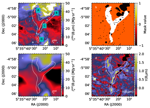
Figure 1: MIR observations of the OMC-3 field. Frame (a) shows the observed 8 $\mu$m surface brightness. Frame (b) shows the masks used, where the value 1 corresponds to the chosen filament region (shown with dashed contours in the other frames) and the value -1 corresponds to masked stars. Frame (c) shows the estimated extended emission, $I^{\rm ext}$, and frame (d) the resulting 8 $\mu$m optical depth. Frame (a) also indicates the four filament fragments that were chosen for further analysis (solid white lines with labels A-D).

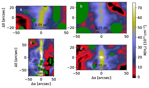
Figure 2: Two-dimensional images of the four OMC-3 filament segments that are marked in Fig. 1a. Each frame shows one segment that is extracted from the column-density map so that the filament runs vertically at the centre of each frame. The green areas correspond to pixels that are masked because of point sources.

Figure 1 shows the MIR data and the derived 8 $\mu$m optical depth map. The strongest MIR absorption is found within a y-shaped region, which can be interpreted as one main filament on the west side and one side filament extending towards the north-east. For further analysis, we selected from this area four isolated filament segments that show the deepest MIR absorption (i.e. correspond to the highest column densities) and are not significantly contaminated by emission from embedded or nearby stars. The segments are labelled with letters A-D in Fig 2a.

The column-density maps of the segments were then extracted as 2D images, where the filaments are aligned vertically. We fitted each individual row as well as the median profile of each filament segment with Eq. (7). The model includes a linear background, the Plummer profile with a possible shift in the direction perpendicular to the filament length, and convolution with a Gaussian beam with FWHM=2.0$\arcsec$ (approximating the Spitzer beam size). The results are shown in Fig. 3 for the filament segment A, based on data within [-90$\arcsec$, +90$\arcsec$] of the filament centre. Corresponding plots for the three other segments can be found in Appendix  B.

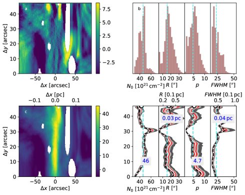
Figure 3: Results of the Plummer fits to OMC-3 filament segment A that was measured using MIR extinction. Frame (c) shows the filament column densities (units $10^{21}$ cm^-2) as a 2D image, the filament running vertically in the plot. The top row contains the median profile. Frame (a) shows the fit residuals. Frame (d) shows the parameter estimates along the filament. The shaded regions correspond to different percentile ranges of MCMC samples: [1, 99]% in dark grey, [10, 90]% in light grey, and [25, 75]% in red. The MCMC median values are plotted as solid white curves. The values from separate $\chi^{2}$ minimisation are plotted with dashed black curves. The vertical dashed light green lines (frame b and frame d) show the median of the parameter values in the individual least-squares fits, while the white half-circles at the top of frame (d) correspond to the fit to the median profile. Frame (b) shows histograms of the parameter distributions based on MCMC samples over all profiles.

The figures also show the filament FWHM values that were calculated from the parameters of the Plummer fits. The $FWHM$ values are usually much more robust than the values of the individual parameters $R$ and $p_{0}$ (Suri et al., 2019). There is no significant correlation between the fitted filament column density (parameter $N$) and the FWHM. If the filament is not well defined (or well matched by the assumed functional form), the parameter $N_{0}$ does not accurately represent the central column density, because of partial degeneracy with the fitted linear background. The median FWHM value of the filament is $\sim$0.05 pc.

3.2 OMC-3 filaments in FIR emission

For comparison with the MIR results, we analysed the column-density maps obtained from Herschel and the combined Herschel and ArTéMiS data. We extracted column densities for the same short filament segments as in the MIR analysis and fitted these with the model of Eq. (7).

We used the LR and HR column-density maps estimated with Herschel 160-500 $\mu$m data and the AR map that also makes use of ArTéMiS data. Figures 4 and 5 show the results for the first filament segment A, using the HR column-density map (angular resolution 20$\arcsec$) and the AR map (angular resolution 10$\arcsec$). The corresponding plots for the other filament segments are shown in Appendix C. The values of $p$ are of the order of $\sim$3, but with significant scatter. The higher-resolution maps result in lower FWHM values, with the exception of segment A.

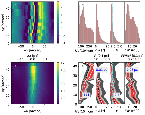
Figure 4: Plummer fits of OMC-3 filament segment A, using the HR column-density map (angular resolution 20$\arcsec$). Frame (c) shows the filament segment as a 2D image (the top row containing the median profile), frame (a) the fit residuals, frame (d) the parameter estimates along the filament, and frame (b) the parameter histograms (cf. description in Fig. 3). The column-density map has an angular resolution of 20$\arcsec$, and the fitted area is [-90$\arcsec$, +90$\arcsec$] in the cross-filament direction.

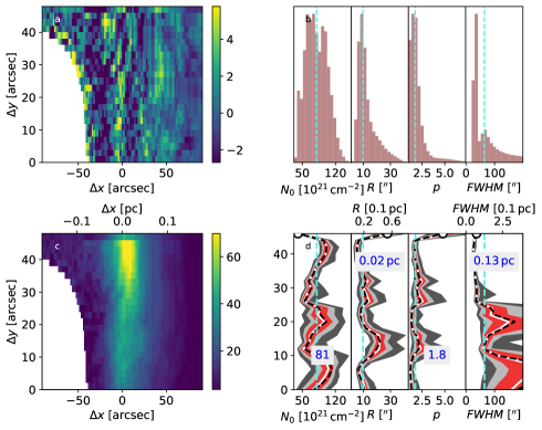
Figure 5: Plummer fits of OMC-3 filament segment A. The figure is the same as Fig. 4 but uses the AR column-density map that is based on combined Herschel and ArTéMiS data and has an angular resolution of 10$\arcsec$.

The above results apply to fits to data within $|r|<90\arcsec$ of the filament centre. To test the sensitivity to the extent of the fitted region, the analysis was repeated by varying the maximum distance between $r_{\rm max}=60\arcsec$ to $r_{\rm max}=210\arcsec$. Figure 6 shows the resulting median parameter values for the four filament segments. In addition to the HR and AR data (20$\arcsec$ and 10$\arcsec$ resolutions), we include here the results using the LR (41$\arcsec$ resolution) column-density map.

The FWHM values obtained from different column-density maps are relatively consistent. The results are similar for the LR and AR maps, and HR data result in only slightly lower values. We also repeated the LR and HR analysis using the column-density maps provided by the Gould Belt Survey, where the maps have resolutions of 36.3$\arcsec$ (Roy et al., 2013) and 18.2$\arcsec$ (Polychroni et al., 2013). The 36.3$\arcsec$ resolution maps showed no noticeable differences to our results with the LR map. The 18.2$\arcsec$ maps resulted in slightly higher FWHM values that match our LR and AR results more closely. These small differences could be caused by differences in the background subtraction (which in the case of the HR map was done close to the filament), the convolution kernels, and even the assumed $\beta$ values ($\beta=2$ in Polychroni et al., 2013).

One clear outlier is segment A in the AR map (Fig. 6g), where the $FWHM$ value increases with increasing $r_{\rm max}$. However, the values appears to be affected by the masked area, which corresponds to the edge of the ArTéMiS coverage (Fig. 5). In the better defined end of the segment, the FWHM values also drop in segment A close to the general $\sim 0.05$ pc level. Segment B also shows larger FWHMs in the LR and AR maps than in the HR map. The widths are smaller in the high-density end and larger in the low-density end, the median in this case picking the larger value.

The MIR data result in FWHM estimates that are even surprisingly close to the values derived from dust emission. However, while all emission maps give values $p\sim 3$ for the power-law index, the MIR results show a much larger scatter. The values are high ($p>4$) for the B and C segments, and, as shown in Figs. 20- 21, the values are consistently high along the entire filament segments.

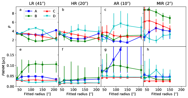
Figure 6: Parameters $p$ (upper frames) and FWHM (lower frames) in fits to OMC-3 LR, HR, and AR maps (based on dust emission) and the MIR maps. Each frame shows results for the four filament segments, A-D, the symbols corresponding to median and the inter-quartile range of the least-squares parameters over the filament length.

4 Analysis of synthetic filament observations

In this section we use the cloud model of Sect. 2.4 to examine sources of potential bias in the dust emission and extinction observations. With the parameters used in the simulations (0.0116 pc pixels, $R=6$ pixels, and $p=3.0$), the model filament has a FWHM size of 0.14 pc or some 72$\arcsec$ at a distance of 400 pc (Sect. 2.4). The synthetic observations were made using a Gaussian beam with $FWHM=24\arcsec$. The beam size and filament properties are roughly similar to those found in some Herschel studies (e.g. Arzoumanian et al., 2011; Rivera-Ingraham et al., 2016; Panopoulou et al., 2022) but the simulations are not intended to directly replicate the OMC-3 observations. In particular, we examine a wider range of models with maximum column densities ranging from $N({\rm H}_{2})=10^{21}$ cm^-2 to $N({\rm H}_{2})=10^{24}$ cm^-2.

4.1 Bias in FIR observations

We look first at FIR observations of a filament illuminated by an isotropic external radiation field. Figure 7 shows the true optical depth profiles and the profiles estimated from synthetic surface brightness maps for filaments of different column density.

The results are almost correct up to $N({\rm H}_{2})\sim 10^{22}$ cm^-2, although $\tau$ is increasingly underestimated. When the column density reaches $N({\rm H}_{2})=3\cdot 10^{22}$ cm^-2, the estimated peak $\tau$ is some 75% of the correct value and $p$ is overestimated by $\sim$4%. The filament FWHM is overestimated by $\sim$30%, and the effect increases with increasing column density. The results were not sensitive to the assumed beam size.

The MBB fits were made with $\beta=2.0$, which is close to the actual value in the dust model. At $N({\rm H}_{2})=10^{22}$ cm^-2, the use of $\beta=1.8$ or $\beta=2.2$ would change the column-density estimates by -22% or +27%, respectively, while the FWHM is affected only at the $\sim$1% level.

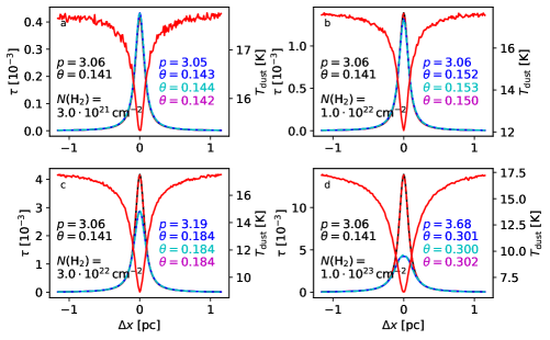
Figure 7: Profiles of optical depth, $\tau$, and dust temperature in the case of model filaments illuminated by an isotropic external field. The black curves show the true optical-depth profiles and the dashed red curves (fully overlapping the black curves) the Plummer functions fitted to those profiles. The blue and dashed cyan lines are, respectively, the optical depth profile derived from synthetic 160-500 $\mu$m surface brightness observations and the Plummer fit to those data. The values of $p$ and FWHM (in parsecs, in the plot marked as $\theta$) are shown for both the true profile (left side, black font) and the estimated (right side, blue font) $\tau$ profiles. The analysis assumes $\beta=2.0$, but FWHM values for $\beta=1.8$ and $\beta=2.2$ are also shown in cyan and magenta, respectively. The assumed beam size is 24$\arcsec$. The dust temperature profiles (solid red curves) are cross-sections of the 3D model and are shown at full model resolution.

Figure 8 shows how the bias in the $p$, $R$, and FWHM estimates increases with column density. For the normal ISRF and fits to the $|r|<0.58$ pc area, the FWHM is at $N({\rm H}_{2})=10^{23}$ cm^-2 overestimated by a factor of two. The bias in $p$ is 20% at $N({\rm H}_{2})=10^{23}$ cm^-2 and more than 50% at $N({\rm H}_{2})=3\cdot 10^{23}$ cm^-2. The fractional errors in $R$ are larger, but even there become significant only beyond $N({\rm H}_{2})=3\cdot 10^{22}$ cm^-2.

Figure 8 also shows results for a radiation field that is a factor of $\chi=10$ or $\chi=100$ stronger at all frequencies. This increases the temperature contrast in the filament but also the average temperature ($\sim$7 K for the $N({\rm H}_{2})=10^{22}$ cm^-2 and $\chi=10$ case). Therefore, a change from $\chi=1$ to $\chi=10$ decreases the systematic errors by a factor of two, and for $\chi=100$ the FWHM estimates remain accurate up to $N({\rm H}_{2})=10^{23}$ cm^-2.

In many observations, fits can only be done using a limited sky area. Figure 8 also shows results for fits within the smaller $r_{\rm max}=0.35$ pc area. This has no effect on the FWHM values, but the errors in $p$ increase. While the observed column-density profile can be fitted with a Plummer function (with parameters different from the true values), it does not match the Plummer profile exactly, since the result depends on $r_{\rm max}$. In the case of noiseless synthetic observations, a wider area always results in more accurate estimates. The situation can be different in real observations if the signal in the filament wings is dominated by noise and emission from unrelated structures.

A change in inclination changes the line-of-sight optical depths but, unlike a true increase of the filament column density, does not affect the temperatures. Appendix D confirms that the inclination has only a minor effect on the extracted filament parameters.

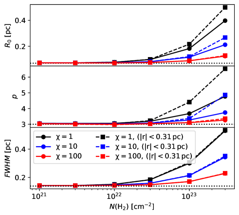
Figure 8: Estimated $p$ and $R$ values and the corresponding FWHM as a function of the peak column density of isotropically illuminated model filaments. The black, blue, and red curves correspond, respectively, to observations of model filaments in a normal ISRF, $\chi=1$, and in stronger fields with $\chi=10$ and $\chi=100$. The solid lines with circles are fits to the model profile at $|r|<0.58$ pc, while the dashed lines with squares are fits to a narrower region, $|r|<0.35$ pc. The horizontal dotted lines indicate the true parameter values in the models.

When the model includes a discrete radiation source, the parameter estimates depend on the distance to the source. Figure 9 shows the true and the recovered profiles at four positions along a model filament. The point source is located behind the filament but, because the filament is optically thin for FIR emission, the results are similar if the source were in front of the filament. At $N({\rm H}_{2})=10^{22}$ cm^-2 and $N({\rm H}_{2})=3\cdot 10^{22}$ cm^-2, the FWHM errors increase towards the point source location but the parameter $p$ is much less affected. Figure 9b demonstrates the central flattening of the recovered $\tau$ profiles, and, as suggested by Fig. 8, the Plummer fits do not follow the actual profile. Schuller et al. (2021) reached qualitatively similar results, although in their case the effects were smaller because of the stronger radiation field ($G_{0}$=1000).

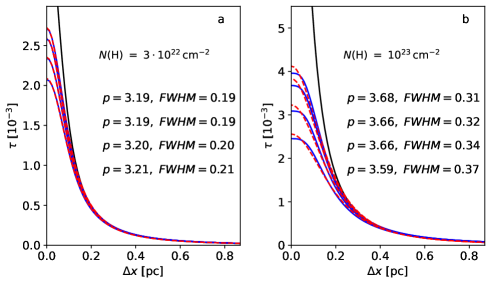
Figure 9: Selected optical-depth profiles along model filaments that are illuminated by a point source. The filament column density is $N({\rm H}_{2})=3\cdot 10^{22}$ cm^-2 (frame a) or $N({\rm H}_{2})=1\cdot 10^{23}$ cm^-2 (frame b). The black curves show the true optical depths, the blue curves the optical depths estimated from FIR observations, and the dashed red curves the Plummer fits to those optical depths. The cross-sections are selected from positions $\Delta y=$0.46, 0.93, 1.39, and 1.86 pc along the filament, when the point source is located at the position $\Delta y$=2.09 pc along the filament and a distance 0.93 pc behind the filament. The curves from top to bottom are in order of decreasing distance to the point source (increasing order of $\Delta y$), and the parameters are listed in the same order (FWHM in units of parsec).

Figure 10 shows how the parameter estimates vary along the filament in the cases of isotropic illumination ($\chi=1$ or $\chi=10$) and the sum of an isotropic field ($\chi=1$) and a point source. The figure confirms the rapid increase of bias at column densities above $N({\rm H}_{2})=10^{22}$ cm^-2. The $p$ values are more sensitive to point-source illumination from one side, while FWHM is more affected when the source is along the line of sight towards the filament. The small bias at the filament ends is caused by these being subjected to the full unattenuated external field.

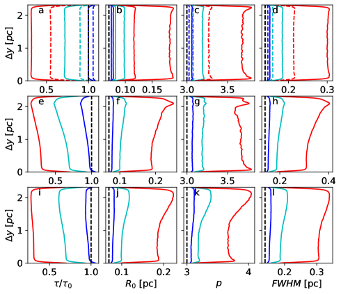
Figure 10: Variation in FIR-estimated parameters along model filaments in cases of: isotropic illumination (frames a-d); a 590 $L_{\sun}$ point source at $\Delta y=2.09$ pc and 0.93 pc behind the filament (frames e-h); and to one side of the filament (frames i-l). The plotted quantities are the ratio between the estimated and true FIR optical depths ($\tau/\tau_{0}$), the Plummer parameters ($R$ and $p$), and the filament FWHM calculated based on these. Each frame shows results for three model filaments with peak column densities $N({\rm H}_{2})=10^{22}$ cm^-2 (blue lines), $N({\rm H}_{2})=3\cdot 10^{22}$ cm^-2 (cyan lines), and $N({\rm H}_{2})=10^{23}$ cm^-2 (red lines). The dashed lines in frames (a)-(d) correspond to cases with a higher isotropic radiation field ($\chi=10$); all other cases include an isotropic field with $\chi=1$. True values are plotted with dashed black lines.

The FIR results can also be affected by changes in dust properties. These could be related to changes in the grain sizes and optical properties, following the formation of larger aggregates and ice mantles (Ossenkopf & Henning, 1994; Ormel et al., 2011; Jones et al., 2016). Figure 11 compares calculations with uniform dust properties to with two two-component models. The single-component models consist of COM, CMM, or AMMI dust. The AMMI model tends to result in the largest systematic errors, especially in the FWHM. The 250 $\mu$m opacity of AMMI is five times higher than for COM, and a similar difference also exists at shorter wavelengths, where dust absorbs energy. The differences are thus caused mainly by changes in the optical depth, since spectral index of AMMI dust ($\beta\sim 2.02$) is similar to the value $\beta=2.0$ that was used in the MBB analysis.

We tested two cases with spatially varying dust properties. The first two-component model consists of CMM dust and a modified CMM, where $\beta$ is decreased from the original 160-500 $\mu$m spectral index $\beta\sim 1.97$ down to $\beta=1.5$. The abundance of the modified dust is calculated as $\tanh(n/[10^{5}\,{\rm cm}^{-3}])$, so that the filament centre consists entirely of the modified dust. This shows the effect of a change in the spectral index, without a net change in the opacity. The results show systematic but relatively minor variations in the filament parameters (Fig. 11).

The second two-component model consists of COM dust in the outer parts and AMMI dust in the inner part. The relative abundance of the AMMI component follows the same density dependence as above. The spectral indices are different ($\sim$2.02 and $\sim$1.83 for AMMI and COM, respectively) but there is a larger difference in the absolute opacities. While the pure AMMI model led to the largest $R$ and FWHM estimates, the COM+AMMI combination leads to the largest $p$ values. This illustrates qualitatively the potential effects from spatial dust property variations. However, the quantitative results will also be sensitive to the radial position and steepness of the transition in dust properties.

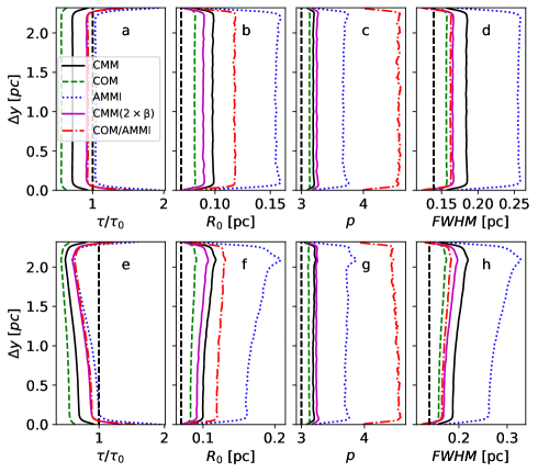
Figure 11: FIR-estimated filament parameters for single-dust models (COM, CMM, or AMMI) and two models with spatial dust-property variations. In $\rm CMM(2\beta)$, the transition is from normal CMM dust in the outer parts to modified dust with $\beta=1.5$ in the inner part. For COM/AMMI, the transition is from COM dust to AMMI dust. The filament column density is $N({\rm H}_{2})=3\cdot 10^{22}$ cm^-2, and the filament is illuminated by an isotropic radiation field (frames a-d) or with a 590 $L_{\sun}$ point source at $\Delta y$=2.09 pc and 0.93 pc to one side of the filament (frames e-h). The plotted parameters are the estimated optical depth relative to its true value ($\tau/\tau_{0}$), the parameters $R$ and $p$ of the fitted Plummer functions, and the resulting filament FWHM estimate.

4.2 Bias in MIR observations

The filament models of Sect. 4.1 were also used to examine how the MIR analysis is affected by in situ dust scattering and emission. Radiative-transfer calculations provide the surface brightness due to 8 $\mu$m dust scattering with the CMM dust model and the thermal emission from stochastically heated grains with the COM dust model. We concentrate here on the systematic effects. Appendix E examines further some effects related to observational noise.

4.2.1 Effect of MIR scattering

For a filament with $N({\rm H}_{2})=3\cdot 10^{23}$ cm^-2, the scattering results in errors of less than $\sim$1% in the estimated $\tau(8\,\mu{\rm m})$. This remains true even if the isotropic radiation field is increased to $\chi=10$ or the default point-source luminosity is increased by a factor of 50. The calculations assume an intensity $I^{\rm bg}$=10 MJy sr^-1 for the background sky. This is similar to the OMC-3 field but still a relatively low value. If the background is higher, the effects from scattering in the cloud would be further reduced.

The importance of scattering increases with increasing column density. For $\tau(8\,\mu{\rm m})<1$, the intensity of the scattered light follows the column-density profile. If the filament is optically thick, the scattered light will peak on either side of the column-density peak, with potentially larger impact of the parameter estimates. However, Fig. 12 shows that for a filament with $N({\rm H}_{2})=10^{24}$ cm^-2, the maximum optical-depth errors remain below 10%, both for an isotropic field $\chi=10$ or a point source with luminosity 50 times the default value. If the isotropic radiation field is increased to $\chi=50$, the errors exceed 20% for a $N({\rm H}_{2})=10^{24}$ cm^-2 filament. If the column density is increased further by a factor of three (to rather extreme values), the errors would exceed 60%. The bias is determined mainly by the optical depth. The optical depth depends on the column density but also the dust properties and would be more than two times higher for the AMMI dust than for the CMM dust was used in Fig. 12.

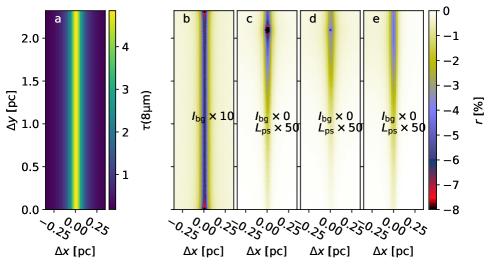
Figure 12: Modelled effect of scattering on the MIR optical-depth estimates towards filament centre. Frame (a) shows the model optical depth, which corresponds to a peak column density of $N({\rm H}_{2})=10^{24}$ cm^-2 with the CMM dust model. The other frames show the relative error in $\tau(8\mu{\rm m})$ estimates. Frame (b) includes only an isotropic radiation field with $\chi=10$. Frames (c)-(e) show the errors, when a point source, with luminosity 50 times the default value, is included at $\Delta y=2.09$ pc and 0.93 pc behind the filament (frame c), in front of the filament (frame d), or to one side.

Figure 13 shows the effect of scattering on the filament parameter in the case of a $N({\rm H}_{2})=10^{24}$ cm^-2 filament illuminated by an isotropic field and a foreground point source. For the default radiation-field values, the bias caused by light scattering is $\sim$1% or less. When the isotropic field is increased to $\chi=20$, the errors in $p$ and FWHM rise to a few per cent. If the point source is made 50 times stronger, the errors exceed $\sim$15%, but only in a small area closest to the point source.

In summary, the scattering in the filament has only a minor effect on the parameter estimation. The effect become visible only if the local radiation field is very strong, the filament has a very high column density, and the background surface brightness is low.

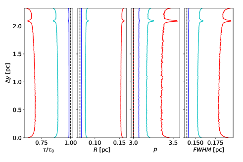
Figure 13: Modelled effect of scattered light on the filament parameters derived from MIR observations. The filament column density is $N({\rm H}_{2})=10^{24}$ cm^-2, and it is illuminated by an isotropic radiation field and a foreground point source. The blue curves correspond to the case of $\chi=1$ for the isotropic component and the point source with the nominal luminosity. The cyan and red curves show, respectively, the results when both radiation-field components are scaled by a factor of 20 or 100. The dashed black lines show the correct values of the parameters.

4.2.2 Effects of MIR dust emission

The effects of the 8 $\mu$m thermal emission from stochastically heated grains ($I^{\rm shg}$) was examined using the COM dust model. Figure 14 shows maps of the dust emission for a $N({\rm H}_{2})=3\cdot 10^{23}$ cm^-2 filament. An isotropic radiation field ($\chi$=1) results in emission at a level of $I_{\nu}(8\,\mu{\rm m})\sim 0.5$ MJy sr^-1. This is not completely negligible if the background sky brightness is low. The 590 $L_{\sun}$ point source has a larger effect, which ranges from less than 1 MJy sr^-1 far from the source to $\sim$100 MJy sr^-1 close to the source. For the column density of $N({\rm H}_{2})=10^{23}$ cm^-2, the surface brightness remains at a similar level, but the morphology is different. The surface brightness follows more closely the column-density distribution, and, for a source behind the filament (Fig. 14 frame c), the intensity peaks towards the centre of the filament, with only a minor dip at $|\Delta x|<0.05$ pc.

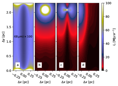
Figure 14: Maps of thermal dust emission $I^{\rm shg}$ calculated for the $N({\rm H}_{2})=3\cdot 10^{23}$ cm^-2 filament model. Frame (a) corresponds to isotropic illumination with $\chi=1$, but the surface-brightness values are multiplied by 100 just for plotting (the same colour bar applies to all frames). The other frames include both the isotropic field and a point source located at $\Delta y=2.09$ pc and at a distance of 0.93 pc in front, behind, or to the left of the filament centre axis (frames b, c, and d, respectively).

Because the thermal emission is stronger and more extended than the scattered light, it could even affect the observer’s estimate of $I^{\rm bg}$. We calculated alternative $\tau$ maps, where the median value of the thermal emission $I^{\rm shg}$ from stochastically heated grains (in the area visible in the Fig. 14) was added to the original $I^{\rm bg}$. The added component is not truly part of the sky background, because it originates within the source itself and preferentially on the observer’s side of the source.

Figure 15 shows the results for $N({\rm H}_{2})=3\cdot 10^{23}$ cm^-2, when the point source is towards one side of the filament. Because the observed sky brightness varies along the $\Delta y$ coordinate, the $\tau$ profiles do not drop to zero in the filament wings. This effect is mostly eliminated by the linear background component that is part of the fitted profile function (Eq. (7)). Nevertheless, the parameter estimates vary by up to 50% with the distance to the point source. Both $p$ and FWHM are more overestimated near the point source, although $p$ drops sharply at the position closest to the point source.

Figure 15 also shows results for a stronger isotropic field with $\chi=10$, where $I^{\rm bg}$ has to take into account the extended emission. The optical depths are now underestimated more, and the especially $p$ shows large bias. Nevertheless, the filament FWHM is overestimated only by some 25%.

Other cases with $N({\rm H}_{2})=3\cdot 10^{23}$ cm^-2 but different radiation fields are shown in Appendix F. If the point source source is directly in front of or behind the filament, its effect is amplified, as more line-of-sight material is heated. The parameter values are then lower at $\Delta y\ga 1$, and the filament disappears close to the projected point-source location, when the dip caused by the background extinction is filled by thermal emission. This happens even earlier for models of lower column density, because the lower opacity reduces the background absorption more than it reduced the thermal emission.

In Appendix F we examine a model with lower column density, $N({\rm H}_{2})=3\cdot 10^{22}$ cm^-2, and higher background intensity, $I^{\rm bg}=100$ MJy sr^-1. Filament parameters are there generally accurately recovered. However, the errors in $p$ and FWHM still reach 30% close to the point source and, if the source is along the line of sight, the filament disappears as an absorption feature.

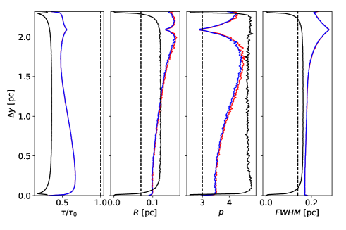
Figure 15: Estimated filament parameters along the $N({\rm H}_{2})=3\cdot 10^{23}$ cm^-2 model filament, when the surface brightness includes 8 $\mu$m thermal dust emission. The filament is illuminated by an isotropic background ($\chi=1$) and a point source at $\Delta y=2.09$ pc and a distance 0.94 pc to one side of the filament (cf. Fig. 14d). Red curves correspond to calculations with the true value of $I^{\rm bg}=10$ MJy sr^-1 and blue curves to a case where the median surface brightness from Fig. 14d is added to the estimate of $I^{\rm bg}$. The black curves are for the case of a $\chi=10$ isotropic radiation field (no point source), with a similarly adjusted $I^{\rm bg}$ estimate.

5 Discussion

We have examined the estimation of the filament properties with observations of MIR extinction and FIR dust emission. In Sect. 5.1, we discuss the observational results on the OMC-3 field. In Sect. 5.2, we concentrate on the radiative transfer models and, based on the models, the systematic errors that may affect the filament observations.

5.1 OMC-3 filament parameters

We analysed four filament segments, named A-D, in the OMC-3 cloud. Based on MIR absorption, the median FWHM widths are $\sim$0.04 pc, with little dependence on the fitted cross-filament extent $r_{\rm max}$. The values were on average consistent between the four segments, but there were also significant variations along the filaments. These are discussed further in Sect. 5.3. The analysis of FIR emission also gave median FWHM$\sim$ 0.03-0.05 pc, but, in the case of segment B, up to $\sim$0.1 pc. FIR emission was analysed using column-density maps with angular resolutions from 10$\arcsec$ to 41$\arcsec$. There were only small differences between the different map versions, the HR version (20$\arcsec$ resolution) resulting in the smallest values, with median values of 0.02-0.04 pc in Fig. 6. Fits to the median profiles gave values that were similar to the median parameter values along the filaments.

Previous Herschel studies have typically found filament widths of $\sim$0.1 pc. Arzoumanian et al. (2011) reported a narrow distribution of $0.10\pm 0.03$ pc in the cloud IC5146, at a distance of 460 pc. These (deconvolved) widths were based on Gaussian fits, and column-density maps at $\sim 37\arcsec$ resolution and 250 $\mu$m surface brightness maps at $\sim 18\arcsec$ resolution gave similar results. Rivera-Ingraham et al. (2016) analysed 29 filaments in 13 separate fields at $d=100-500$ pc distances, the analysis of column-density maps of 41$\arcsec$ resolution resulting in widths of $0.13\pm 0.05$ pc. In the above papers, the fits were done to the mean (or median) radial profile of an entire filament that was detected with automated methods, using DisPerSE (Sousbie, 2011) in the case of Arzoumanian et al. (2011) and getfilaments (Men’shchikov, 2013) in the case of Rivera-Ingraham et al. (2016). Arzoumanian et al. (2011) extended Herschel studies to 599 filaments in eight regions at 140-460 pc distances, the distribution again peaking at $\sim 0.1$ pc with an interquartile range of 0.07 pc. However, based on Herschel data in Arzoumanian et al. (2019), Panopoulou et al. (2022) concluded that the filament width estimates also depend on the source distance and appear to be 4-5 times the beam size. Thus, the widths would increase from less than 0.1 pc in the closest fields (e.g. Taurus and Ophiuchus) to almost 0.3 pc at $\sim$800 pc (the IC5146 cloud). This scaling appeared to hold for regions of very different types, from the low-density Polaris field to the Orion-B cloud with active star formation. Some distance dependence was also noted in Rivera-Ingraham et al. (2016).

Although deconvolution by a larger telescope beam increases uncertainties, with perfect observations of perfect Plummer profiles, the FWHM estimates should not depend on the resolution of observations. Indeed, in our analysis, the factor of 20 range in the angular scales is not associated with corresponding systematic changes in the estimated filament widths. The average FWHM were at or below 0.05 pc for all maps, although Herschel data could in some cases lead to higher values FWHM$\sim$0.1 pc (segments A and B, Fig. 6). The values are lower than those reported in Panopoulou et al. (2022) for fields at similar distances (including Orion B with FWHM$\ga$0.15 pc), and do not match distance/resolution dependence reported there. In all the above studies, the column densities were based on the modelling of dust emission with a single-component MBB. Howard et al. (2019) and Howard et al. (2021) used the PPMAP method (Marsh et al., 2015) to analyse Herschel and SCUBA-2 observations of filaments in the Taurus and Ophiuchus clouds. They noted that the use of the PPMAP method, which takes temperature variations into account, resulted in a reduction in the estimated filament widths. Our results were also roughly constant with respect to the size of the fitted cross-filament area. Therefore, even if the extent of the fitted area typically increases with the target distance, that should not necessarily lead to larger FWHM estimates.

Filaments in the OMC-3 region were already investigated by Schuller et al. (2021), who used Herschel 160-500 $\mu$m and ArTéMiS 350 $\mu$m and 450 $\mu$m data (different observations from the ArTéMiS data analysed in Mannfors et al. (2022)). The ArTéMiS surface-brightness data and Herschel temperature information at 18.2$\arcsec$ resolution were combined to a column-density map with 8$\arcsec$ resolution. This resulted in filament FWHM estimates of 0.06$\pm$0.02 pc. These values are similar to our AR results, where (ignoring the outlying values of segment A) the median values range from 0.04 pc to $\sim$0.1 pc (Fig. 6g). While Schuller et al. (2021) studied long, automatically detected filaments, our analysis is limited to short segments at the highest column densities.

In addition to FWHM, the values of the asymptotic power-law index, $p$, of the fitted Plummer function are of interest. The Herschel and combined Herschel and ArTéMiS data gave typically values $p=2-5$, with some variations depending on the extent of the fitted area. These suggest that nearby cloud structures are affecting the fits in the tails of the profile function (cf. Sect. 5.3). Compared to FWHM, the individual $p$ and $R$ values could be measured less precisely. Especially the MIR $p$ values showed a large scatter, which could be caused in part by changes in the local MIR radiation field. The MIR $p$ estimates are similar for different values of $r_{\rm max}$, which suggests that individual point sources within that area do not have a strong effect on the results.

5.2 Systematic errors in filament parameters

We used radiative transfer simulations to study error sources in the analysis of MIR and FIR observations. In the following we discuss their relative importance and the potential effects on the OMC-3 results.

5.2.1 MIR observations

Dust scattering and thermal dust emission are potential error sources in the analysis of MIR extinction. They depend on the local radiation field and are significant at high column densities. We assumed in the tests a background level of 10 MJy sr^-1. However, if the background level is higher, the effects of local emission and scattering will be reduced.

For dust scattering, errors reached tens of per cent only if the column density is $N({\rm H}_{2})\sim 10^{24}$ cm^-2 or higher. The intensity of the isotropic background also had to be a factor of $\chi=100$ above the normal ISRF or the luminosity of a point source at $\sim$1 pc distance had to be of the order of $\sim 10^{4}$L_☉. Thus, scattering should not be a significant source of errors in the OMC-3 field. Scattering would tend to decrease the $\tau$ estimates, increase the $p$ estimates, and lead to overestimations of the filament FWHM (Fig. 13). These effects are more pronounced close to point sources, especially if the source is on the line of sight towards the filament. The presence of such point sources would be evident in the observed maps, although their effect can extend over distances of several parsecs.

The MIR scattering depends strongly on the grain properties. The so-called coreshine, which is observed at 3-4 $\mu$m wavelengths towards many dense cores, has indicated surprisingly strong MIR scattering. This requires strong dust evolution relative to diffuse clouds (Steinacker et al., 2010; Pagani et al., 2010; Juvela et al., 2012c; Steinacker et al., 2014b; Lefèvre et al., 2014). Lefèvre et al. (2016) investigated the 8 $\mu$m scattering towards the pre-stellar, high-column-density core of L 183, where the estimated intensity of the scattered light was hundreds of kJy sr^-1. This corresponds to the scattering in a more or less normal ISRF, and the high scattering efficiency could be explained by large aggregate grains. The L 183 observations (and the possibility of very large aggregates) suggests that the scattered signal could be stronger than in our simulations. If the scattered light is in L 183 at a level of $\sim 0.1$ MJy sr^-1, scattering could cause noticeable errors in MIR observations of high-mass star-forming regions, where the radiation fields are much stronger.

In our models, the local thermal dust emission was a more significant factor than the scattering. For the high column density of $N({\rm H}_{2})\sim 10^{24}$ cm^-2 filament, the emission effects were tens of per cent, both in the case of the normal ISRF and in the case of the 590 $L_{\sun}$ point source. This led to the filament optical depths being underestimated and the individual filament parameters ($p$, $R$, FWHM) to be overestimated. The magnitude of the effects depends strongly on the presence of local radiation sources (Fig. 13). If there is a point source on the line of sight towards the filament, the thermal emission can completely mask the MIR absorption (Appendix Sect. F). Quantitatively, these effects are sensitive to the filament column density, the level of the background surface brightness, and the location of the point source relative to the filament (Fig. 14). In the comparison to the models, one must also take into account that observations tend to underestimate the true column densities.

Scattering is not only a source of errors but can itself be used to study filaments at high angular resolution. At near-infrared wavelengths the scattering is stronger (in absolute terms and relative to the in situ thermal emission) but the larger optical depths complicate the analysis (Juvela et al., 2012b; Malinen et al., 2013). Scattering may also be measurable at MIR wavelengths, above the MIR absorption (e.g. Steinacker et al., 2014b; Lefèvre et al., 2014). However, this requires a low background sky brightness, such as found at high Galactic latitudes (Steinacker et al., 2014a).

5.2.2 FIR observations

Far-infrared analysis of Sect. 3.2 is affected especially by the bias of column-density estimates, which is caused by temperature variations in the source and the analysis using the single-temperature MBB model. Appendix G shows that these effects can be easily demonstrated even without complex modelling.

In the radiative-transfer simulations of Sect. 4, the column-density estimates vary depending on the data resolution (beam sizes), the analysis method, the temperatures, and dust optical properties. It can be instructive to compare the peak optical depths obtained at different resolutions and with different methods. Table 4 lists values for the $N({\rm H}_{2})=10^{22}\,{\rm cm}^{-2}$ model. Since the filament FWHM is quite large, $\sim 72\arcsec$, the peak values of the 40$\arcsec$ and 20$\arcsec$ maps differ only little. Shorter wavelengths are more sensitive warm dust, tend to bias the temperatures more upwards, and result in lower $\tau$ values. In Table 4 the effect is the opposite for $\beta=1.8$, because the simulation used a dust model with $\beta\sim 1.95$. A modest increase in the assumed $\beta$ (to a value above the $\beta$ in the simulations) can even negate the natural tendency to underestimate the column densities. When real observations are analysed, the precise value of $\beta$ is unknown. However, because $\beta$ affects all column-density estimates similarly, its effect on the observed filament profiles is limited - as long as $\beta$ does not change significantly as a function of the filament radius.

Table 1: Comparison of peak 250 $\mu$m optical depths estimated with different analysis methods. The estimates are based on synthetic surface-brightness maps of the $N({\rm H}_{2})=10^{22}\,{\rm cm}^{-2}$ filament model.

Case	Beam	$\beta$	$\tau^{\rm max}(250\,\mu{\rm m})$	Rel. error
	[$\arcsec$]		$[10^{-3}]$	[%]
true	6	–	1.49	0.00
MBB	6	1.8	1.11	-25.77
MBB	24	1.8	1.04	-29.99
HR	18	1.8	1.04	-30.34
HR	18	2.0	1.33	-10.48
HR	18	2.2	1.71	14.61
HR (w)	18	1.8	1.00	-32.54
HR (w)	18	2.0	1.32	-11.46
HR (w)	18	2.2	1.73	16.05
LR	40	1.8	0.98	-33.98
LR	40	2.0	1.22	-17.85
LR	40	2.2	1.51	1.64
LR (w)	40	1.8	0.96	-35.27
LR (w)	40	2.0	1.22	-18.42
LR (w)	40	2.2	1.52	2.30

The bias of the column-density estimates increase with column density and exceeded a factor of two at $N({\rm H}_{2})=10^{22}\,{\rm cm}^{-2}$ (Fig. 7). Since these errors are correlated with the column density, they also affect the observed filament profiles. The parameters $p$, $R$, and FWHM are all biased upwards. Unlike in MIR observations, a stronger isotropic radiation field decreases the errors by reducing the amount of very cold dust. In the normal ISRF, the systematic errors of filament FWHM reach 50% when the column density exceeds $N({\rm H}_{2})=10^{23}\,{\rm cm}^{-2}$. In a $\chi=10$ field, the errors are less than half of this, and are they are further halved in a $\chi=100$ field. This means that the errors can be of similar magnitude in a low-mass star-forming region (low column density and low radiation field) as in a high-mass star-forming region (high column density and high radiation field). The errors in $R$ and $p$ also depend on both the column density and the radiation field, and can reach 50% for a $N({\rm H}_{2})=10^{23}\,{\rm cm}^{-2}$ in the normal ISRF (Fig. 10). A point source has a similar effect, the errors increasing close to the source and with only a small dependence on the source location (on the line of sight vs to one side of the filament).

The maximum column density of the OMC-3 filaments is in MBB analysis $N({\rm H}_{2})\sim 10^{23}\,{\rm cm}^{-2}$, but the true column density could be even a few times higher. Because the quiescent parts of the filament are likely to be subjected to a radiation field of at most $\chi\sim 100$ (Mannfors et al., 2022), and the effects of MIR scattering are likely to be insignificant. The models predict a more significant role for the MIR dust emission. Figure 15 indicated a $\sim$25% effect for an isotropic radiation field with $\chi=10$. This requires the extended thermal emission to also be taken into account in the $I^{\rm bg}$ estimates. In observations this happens automatically (to some accuracy), and the local thermal emission need not be separated from other contributions to $I^{\rm bg}$. The fact that the OMC-3 FIR and MIR observations resulted in similar FWHM estimates also suggests that the systematic errors of the MIR analysis are unlikely to amount to tens of per cent.

Filaments are located inside dense clouds, which significantly reduces the UV flux that reaches the filament. Most of the 8 $\mu$m emission would then originate in extended regions, and, unlike in our simple models, the emission would be mostly uncorrelated with the filament structure. This will reduce the systematic errors in the filament parameters. A second important factor is the abundance of polycyclic aromatic hydrocarbons and other very small grains (Draine, 2003). If these have already partly disappeared within the filament (e.g. by sticking onto larger grains), the MIR emission would be suppressed. Based on our models, FIR analysis could overestimate the width of $N({\rm H}_{2})\sim 10^{23}\,{\rm cm}^{-2}$ filaments by tens of per cent in the normal ISRF. However, a stronger radiation field reduces the errors to $\sim$10% level, which is within the uncertainties of the MIR versus FIR comparison (Fig. 6). Therefore, although the models show the possibility of significant systematic errors in all observations, there is no contradiction in the approximate agreement between the OMC-3 MIR and FIR estimates.

5.3 Reliability of profile fits

Based on synthetic observations of magnetohydrodynamic cloud simulations, Juvela et al. (2012a) concluded that, at the nominal Herschel resolution, the filament parameters could be recovered reliably only up to $\sim$400 pc (assuming $\sim$0.1 pc filaments). OMC-3 is at this limit and the filaments are partly narrower than 0.1 pc. Nevertheless, the angular resolution of at least the MIR and AR maps should be sufficient for the profile analysis.

In addition to systematic errors, the results show significant random fluctuations, especially in the $p$ and $R$ estimates. Some fits resulted in values $p\ga 5$ that are inconsistent with most physical filament models. Individual $p$ and $R$ values are more difficult to measure because a larger value of $p$ can in Eq. (6) be compensated with a larger value of $R$, the fit still recovering the same FWHM and generally fitting the observed profile. The parameter $R$ probes the structure in the inner part of the filament and is dependent on the data being able to resolve those smaller scales. Conversely, $p$ probes the asymptotic behaviour at large distances and is sensitive to nearby cloud structures and the general background fluctuations.

The error distributions of the parameters (including FWHM) are often asymmetric for the individual profiles, with the MCMC estimates showing a long tail to high values (cf. Fig. 19). The overall dispersion along the segments (as shown by the histograms e.g. in Fig. 3b) give an empirical estimate for the total uncertainty. Our data also contain missing values, which affect the reliability of MIR profiles (e.g. Fig. 3) and the analysis of the AR map of the filament segment A (Fig. 5). The missing data also bias the median profiles. Rather that rejecting all profiles that contained missing values (which could be almost all of the data), the median values were calculated over the remaining pixels. Therefore, at a given distance from the filament centre, the median value is based on different sections along the length of the filament, leading to random errors in the median profile.

Figure 16 shows examples of the fits to the OMC-3 filament segment A, based on the MIR, HR, and AR column-density estimates. Most MIR profiles do not have data around offset $\Delta x=30\arcsec$ but in this case this does not have a major effect on the fits. MIR profiles also tend to show a dip around $\Delta x=-30\arcsec$, which could be caused by imperfections in the column-density estimation (e.g. dust to nearby sources), or random column-density fluctuations. These fits are associated with high values of $p\sim 5$. In comparison, the profile at offset $\Delta y=30\arcsec$ along the filament (red curve) decreases rather than increases towards negative $\Delta x$, and has $p\sim 1.6$. For the maps HR and AR based on dust FIR emission, the fitted profiles match better the observed profiles. However, the effect of the missing data is clear in the AR results, where the observations at $\Delta y$=10 and 20 arcsec (i.e. the profiles most affected by missing values, cf. Fig. 5c) provide only weak constraints at negative $\Delta x$ values. This leads to degeneracy between the Plummer and the background parameters, the background is underestimated at negative $\Delta x$ offsets, and the fit results in abnormally large FWHM values.

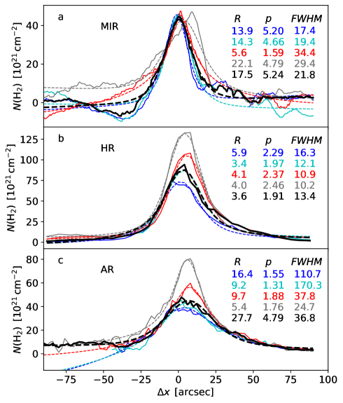
Figure 16: Plummer fits for selected cross-sections of the OMC-3 filament segment A. The three frames correspond to the MIR, HR, and AR column-density maps, respectively. Each frame shows individual profiles for the offsets $\Delta y$=10, 20, 30, and 40 arcsec (cf. Fig. 3-5; blue, cyan, red, and grey lines, respectively) and the median profile (thick black lines). The best-fit Plummer profiles are plotted with dashed lines of the same colour, and $R$, $p$, and FWHM values of the fits are listed in the frames.

Large $p$ values are also observed for some other dust emission data, typically in fainter and less clear parts of the filaments. They can be related to interference from nearby cloud structures, which can be other filaments or clumps (e.g. northern part of filament B, Fig. 23) or diffuse emission that appear as an extension of the filament itself (e.g. segment C, $\Delta x\sim 60\arcsec$, Fig. 24). However, the filament segment D is associated with large values $p\geq 4$ over its full length. Figure 17 shows examples of the individual profiles. The main feature (in HR and AR maps) is a dip at negative $\Delta x$ values. This is similar to the one seen in Fig. 16 and similarly appears to be the origin of the large $p$ values. The situation is worst for the $\Delta x=10\arcsec$ profile, where the background also curves up at positive $\Delta x$ offsets, raising the $p$ value above nine. This suggest that the background might need to be modelled using a second order polynomial, although $p$ would be partly degenerate with an second order background term.

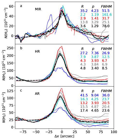
Figure 17: Selected cross-sections of the OMC3-filament segment D. These correspond to HR and AR data (blue and red lines, respectively) and the offsets $\Delta y$=10 and 25 arcsec, where the $\Delta y$=10 arcsec profiles have the lower column density. The dashed lines are the best-fit Plummer profiles with the parameters listed in the figure.

Figure 18 compares the results that are based on the MIR, HR, and AR data on the filament segment D and six versions of the fitted profile function. The row B corresponds to our default model in Eq. (7), which has six parameters: three for the Plummer function itself, one allowing a shift along the $\Delta x$ axis, and two parameters describing the linear background. In Fig. 18, one of the alternative fits omits the shift (row A) and one adds the second order term to the background component (row C). So far all fits assume that the filament profiles are symmetric, which is only approximately true for the selected segments. In Fig. 18, we also show results for asymmetric Plummer functions (separate $R$ and $p$ parameters on each side of the peak) that are combined with a background modelled as a linear first order (row D) or a second order (row E) polynomial.

If the filament shifts in the $\Delta x$ direction at small scales, the omission of the $\Delta r$ term in Eq. 6 should lead to larger FWHM values. No such effect is seen in Fig. 18, although this could still play a role in fits of longer and more fragmented filaments. The addition of the second order background term (figure row C) reduces the $p$ values significantly from $p\sim 5$ to $p\sim 2.5$. The $R$ values are also smaller, but the mean value and the scatter of the FWHM values has increased. When the second order background term is included in the asymmetric Plummer fits, the results are much less affected and especially the FWHM values remain practically unchanged (row E vs row B). With the exception of the row C, the FWHM values are thus similar for all the alternative fits.

In Fig. 18, the fits have between five and nine free parameters. In these calculations, we also added penalties for values $R<0.005$ pc and $p>8$. The AR results were somewhat sensitive to the $R$ threshold, because the filament widths are not much larger than the beam size and unresolved filaments can result in small $R$ values. The FWHM estimates from the LR maps could thus be even more sensitive to any priors that are used. Accurate beam models are also important, since they are used to deconvolve the observations. The LR beam is well defined, while the effective beams of the HR and AR maps depend on the way these maps are constructed. The HR column density is based on a combination of intermediate maps that have different angular resolutions and different sensitivity to temperature variations. The AR map is the combination of data from two instruments, and the effective beam could be affected by calibration differences or imperfections of the feathering procedure.

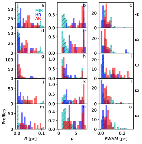
Figure 18: Alternative fits of the filament segment D. The histograms show the distributions of the $R$, $p$, and FWHM parameters that are estimated from the MIR, HR, and AR maps (cyan, blue, and red histograms, respectively). The rows are for alternative models of the profile function, where row B corresponds to our default model. In the other fits, row A omits the shift of the filament centre, row C adds a second order term to the background, row D fits two-sided Plummer functions with linear background, and row E fits two-sided Plummer functions with a second order polynomial for the background.

6 Conclusions

We have studied four filament segments in the OMC-3 cloud in Orion, using observations of MIR extinction and FIR dust emission and with the goal of measuring the filament widths. The Herschel FIR data were converted to column-density maps at 20$\arcsec$ (LR maps) and 41$\arcsec$ (HR maps) resolution, as well as an additional map of 10$\arcsec$ resolution from combined Herschel and ArTéMiS 350 $\mu m$ observations (AR map). In addition to using observational results from the OMC-3 filaments, we performed radiative transfer simulations to investigate sources of systematic errors that could affect the measurement of filament profiles. The study led to the following conclusions:

1. The OMC-3 filament segments have FWHM values of 0.03-0.05 pc. Similar values are obtained with the three column-density maps derived from FIR observations (10-41$\arcsec$ angular resolution) and based on the MIR extinction map ($\sim 2\arcsec$ resolution). In the LR and AR maps, the estimated width was only higher in segment B and (partly) in segment A, with $FWHM\sim 0.1$ pc.

2. The MIR results showed little dependence on the extent of the fitted area, which was varied between 60$\arcsec$ and 210$\arcsec$ maximum distances from the filament centre. Some variation was observed due to map edges and, to a lesser extent, due to the influence of unrelated background structures. The results are based on Plummer fits, where the model itself includes terms for a linear background.

3. When estimated from FIR data, the values of the asymptotic power-law index, $p$, in the Plummer function were $\sim 2-5$, with an average value of $p\sim 3$. The estimates derived from MIR extinction had a large scatter, and the median values of the four segments ranged from $p\sim 3$ to as high as $p\sim 8$.

4. The FWHM estimates are quite robust, even when the individual Plummer parameters, $p$ and $R$, show a large scatter. This applies to both MIR and FIR analysis.

5. Synthetic observations of model filaments were analysed. The MBB fits to 160-500 $\mu$m dust emission led to the expected underestimation of column densities. The error exceeded $\sim 50$% above $N({\rm H}_{2})=3\times 10^{23}$ cm^-2 but depended on the dust properties.

6. A similar bias exists in the filament parameters derived from FIR dust emission. For a $N({\rm H}_{2})=10^{23}$ cm^-2 filament heated by the normal ISRF, the FWHM is overestimated by more than 50%. However, the error decreases by more than a factor of two if the radiation field is ten times stronger and the dust temperatures correspondingly higher. The errors also decrease rapidly at lower column densities.

7. The effect of point sources on the FIR analysis is qualitatively similar to the isotropic field, systematic errors increasing closer to the source. There is only a minor dependence on the source location: a source along the line of sight versus a source to one side of the filament.

8. The accuracy of the MIR extinction analysis is affected by the uncertainty of the foreground emission and the potential effects of MIR dust scattering and emission.

9. In the models, MIR scattering shows only minor effects. The errors in filament parameters reach 10% only at very high column densities ($N({\rm H}_{2})\sim 10^{24}$ cm^-2) and in strong radiation fields ($\chi>10$). Errors are larger near luminous point sources, whose presence should be clearly visible in the maps. Scattering is sensitive to dust properties, and strong grain growth could increase its effects by a factor of several.

10. Thermal MIR emission is, in our models, a more significant error source than MIR scattering. In a $N({\rm H}_{2})=3\times 10^{23}$ cm^-2 model filament, errors already reach the 10% level in the normal ISRF or within a 1 pc distance of a 590 L_☉ point source. Errors are still of the same order of magnitude even in a stronger isotropic radiation field of $\chi=10$. However, if the diffuse UV field is attenuated by the surrounding cloud or the abundance of very small grains is lower inside the filament, the significance of MIR emission is correspondingly decreased.

The estimated widths of the OMC-3 filaments were roughly equal between different tracers and observations of different angular resolution. This is encouraging, considering the many potential sources of systematic errors. However, it also further highlights the differences between the dust filaments and the narrower fibres that are observed in spectral lines. High-resolution comparisons of the dust and gas tracers, within the same sources, are needed to understand these differences and the exact role of filaments in the star-formation process.

Appendix A Test of the fitting routines

The profile function of Eq. (7) was fitted with a least-squares routine and with a MCMC routine. Figure 19 shows results for the analysis of a synthetic dataset. The inputs consist of a set of ideal profiles, which match the model setup, and white noise that is varied from 1% to 20% of the filament peak value. For illustration, we fix the pixel size to 6$\arcsec$ and the data resolution (beam size) to 24$\arcsec$. The profile parameters are varied in the ranges $R=18-30\arcsec$ and $p=1.6-4.4$. The simulation is not concerned with the way the synthetic column-density observations are obtained (emission or extinction), only on the noise effects in the actual profile fitting.

The figure shows that the parameter uncertainty depends not only on the noise level but also on the values of $R$ and $p$. For example, $p$ is correlated with $R$, and its uncertainty is much higher when the true value of $p$ is higher. At high noise levels, the MCMC mean value tends to be above the least-squares solution, because of the skewed error distribution (and the used $p\geq 1$ constraint). Compared to the individual parameters, the FWHM estimate is generally more accurate, but its uncertainty still increases significantly when the value of $p$ is low.

The results depend on the size of the analysed region, and fits to a narrower area around the filament will naturally lead to higher errors (especially for low $p$). However, the errors in real observations can be dominated by structured background emission rather than observational noise.

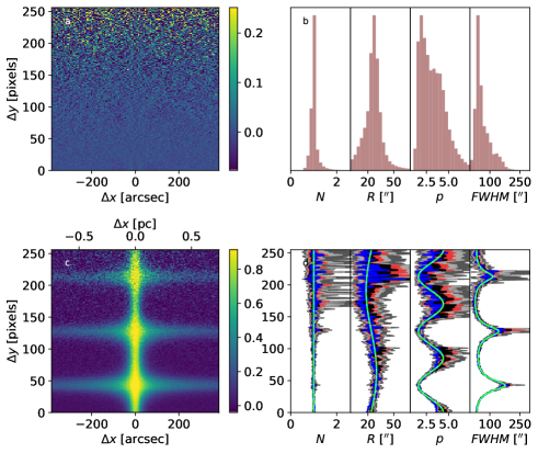
Figure 19: Fits of synthetic filament profiles. Frame (c) shows 256 generated profiles, where the noise relative to the filament peak increases logarithmically from 1% at the bottom (at $\Delta y$=0) to 20% at the top (at $\Delta y$=255). The residuals of the least-squares fits are show in frame (a). Frame (d) shows the recovered parameter values, where the light-green lines correspond to the true input values, and the least-squares estimates are plotted in blue. For the MCMC calculations, the black lines show the mean of the MCMC samples and the red, light-grey, and dark-grey bands correspond to the [25, 75], [10,90], and [1, 99] percentile intervals, respectively. Frame (b) shows histograms corresponding to MCMC samples along the full length of the filament.

Appendix B Additional figures of fits to OMC-3 MIR data

Section 3.1 discussed the filament properties based on OMC-3 MIR observations, and Fig. 3 showed the estimated parameters for the filament segment A. Here Figs. 20-22 show the corresponding results for the other segments B-D.

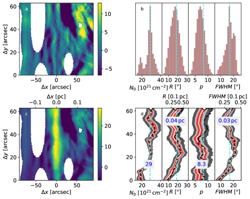
Figure 20: Plummer fits of MIR absorption. As Fig. 3 but for OMC-3 filament segment B.

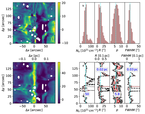
Figure 21: Plummer fits of MIR absorption. As Fig. 3 but for OMC-3 filament segment C.

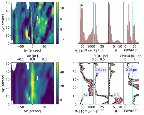
Figure 22: Plummer fits of MIR absorption. As Fig. 3 but for OMC-3 filament segment D.

Appendix C Additional figures of fits to OMC-3 FIR data

Section 3.2 presented results of Plummer fits to column-density data that were obtained from Herschel and ArTéMiS FIR measurements, including figures for the filament segment A. We present here the corresponding figures for segments B-D. Figures 23-25 show the results based on Herschel data ($20\arcsec$ map resolution and fits to an area [-90$\arcsec$,+90$\arcsec$] around the filament centre). The corresponding results for the combined Herschel and ArTéMiS data are plotted in Figs. 26-28.

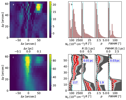
Figure 23: Plummer fits of Herschel column-density data at 20$\arcsec$ resolution. As Fig. 4 but for OMC-3 filament segment B.

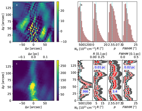
Figure 24: Plummer fits of Herschel column-density data at 20$\arcsec$ resolution. As Fig. 4 but for OMC-3 filament segment C.

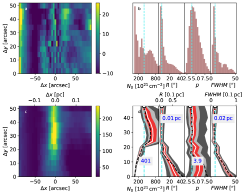
Figure 25: Plummer fits of Herschel column-density data at 20$\arcsec$ resolution. As Fig. 4 but for OMC-3 filament segment D.

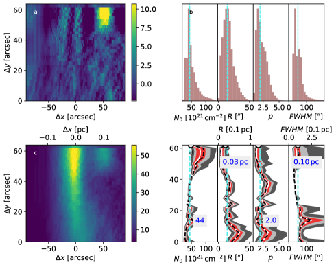
Figure 26: Plummer fits of combined Herschel and ArTéMiS data at 10$\arcsec$ resolution. As Fig. 5 but for OMC-3 filament segment B.

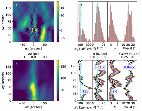
Figure 27: Plummer fits of combined Herschel and ArTéMiS data at 10$\arcsec$ resolution. As Fig. 5 but for OMC-3 filament segment C.

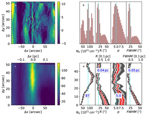
Figure 28: Plummer fits of combined Herschel and ArTéMiS data at 10$\arcsec$ resolution. As Fig. 5 but for OMC-3 filament segment D.

Appendix D Effect of filament inclination

We tested the effect of different viewing angles using filament models with column densities $N({\rm H}_{2})=3\cdot 10^{22}$, $10^{23}$, and $3\cdot 10^{23}$ cm^-2 perpendicular to the filament axis. By increasing the inclination from zero to 70.5 degrees, the line-of-sight column density increases by a factor of three. Therefore, the comparison to the $N({\rm H}_{2})=10^{23}-10^{24}$ cm^-2 models shows the relative importance of the true versus line-of-sight column densities.

Figure 29 shows that the effect of inclination is much smaller than that of the actual filament column density. At higher inclinations, $R_{\rm 0}$ and FWHM show no indication of rising close to the values of the filaments with the same line-of-sight column density observed at zero inclination. This is not surprising, given that the relative amounts of dust at different temperatures is not affected by the inclination, and the 160 $\mu$m emission remains optically thin ($\tau\sim 0.3$ at $N({\rm H}_{2})=10^{24}$ cm^-2). At the highest inclinations, the results may also be affected by edge effects, as the line of sight enters and leaves the model volume (on the front and back border of the model volume) relatively close to the filament axis, where the density is not negligible.

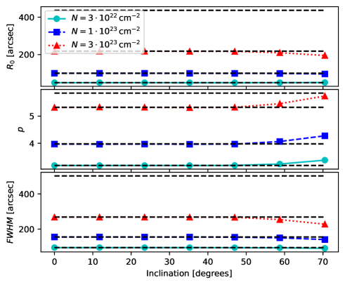
Figure 29: Dependence of filament parameters on the column density and inclination of model filaments. The cyan, blue, and red curves and symbols show, respectively, parameter estimates at column densities $N({\rm H}_{2})=3\cdot 10^{22}$ cm^-2, $N({\rm H}_{2})=10^{23}$ cm^-2, and $N({\rm H}_{2})=3\cdot 10^{23}$ cm^-2 as functions of the filament inclination. Zero inclination corresponds to the perpendicular view direction and 70.5 degrees to a factor of three higher line-of-sight column density. For reference, the horizontal black dashed lines show the zero-inclination values for the three column densities and additionally for $N({\rm H}_{2})=10^{24}$ cm^-2 (the uppermost lines).

Appendix E Tests of fitting mid-infrared filament profiles

Errors in the determination of the foreground surface-brightness component $I^{\rm fg}$ will affect not only the level of optical-depth estimates but also cause uncertainty in the filament profiles. We examined these effects with simulated observations, where the optical depth follows a Plummer profile. The dimensionless parameters of the Plummer model are $\tau_{\rm 0}$=4.0 for the peak optical depth, $R_{\rm 0}$=3.0 for the central flat region, and $p_{\rm 0}$=2.5 for the asymptotic power law. The filament is seen against extended background $I^{\rm bg}$=10.0 units and the foreground is set to $I^{\rm fg}$=2.0 units. We simulate a piece of a filament where the ridge optical depth is further modified by a Gaussian function, dropping to 40% of the maximum at both ends.

The simulation consists of synthetic observations with two sources of error. The first is the observational noise and the second an error in the estimated level of the extended emission component $I^{\rm ext}$. For simplicity, we use the same noise value for both components. Although $I^{\rm ext}$ can often be estimated based on a large number of pixels, the interpolation across the extincted regions is uncertain, and the uncertainty of $I^{\rm ext}$ could be larger or smaller than the uncertainty of a single surface brightness measurement. The error of the $I^{\rm fg}$ estimate follows from the observational noise, because it is here estimated from Eq. (8). To keep the statistics similar to observations, $I^{\rm fg}$ is estimated using only 64 points along the filament length. However, to gather more statistics for the following plots, the rest of the simulation is done using 1024 independent profiles along the filament.

First, Fig. 30 shows examples of filament profiles that are derived from noisy observations with 0.2 units of noise in both surface brightness and $I^{\rm ext}$ values. Since Eq. (8) is used, the optical depth estimate is always defined. On the other hand, there is a small bias whereby the optical depth at the filament centre tends to be underestimated. Because this bias is largest when the observed surface brightness approaches the assumed $I^{\rm fg}$ value, the recovered profiles tend to be flatter in the centre and thus also have FWHM values that are slightly larger than for the true filament profile.

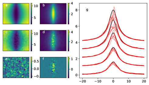
Figure 30: Example simulated MIR observations of a model filament. Frames (a) and (b) show the ideal absorption and the corresponding true optical depth image. Frames (c) and (d) are the corresponding noisy realisations, with noise 0.2 units for both surface brightness observations and for the determination of the level of $I^{\rm ext}$, and frames (e) and (f) show the differences between frames (a) and ()b and between frames (b) and (d). The black curves in frame g show examples of profiles, from the end of the filament (bottom curve) to the centre of the filament length (uppermost curve). The curves are offset along the y axis for better readability. For each ideal profile, there are ten realisations of the profiles derived from noisy observations.

To study the accuracy of the recovered filament parameters, we simulated further four situations. First, the noise values were set to either 0.2 or 0.55 units. Second, in addition to direct application of Eq. (8), we also tested a case where $I^{\rm fg}$ is set based on the minimum observed surface brightness value. The results in Fig. 31 suggest that the method used for $I^{\rm ext}$ estimation has only little effect. On the other hand, with increasing noise the central optical depth becomes significantly underestimated while the computed FWHM values are biased upwards.

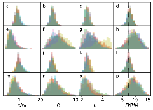
Figure 31: Histograms of extracted filament parameters for simulated observations. The first three columns show the recovered central optical depth relative to the true value, $\tau/\tau_{0}$, and the parameters $R$ and $p$. The last column contains the FWHM values computed from the Plummer parameters. In frames (a)-(h), $I^{\rm fg}$ is estimated with Eq. (8), in frames (i)-(p) simply based on the minimum observed value. The noise values are 0.2 in frames (a)-(d) and (i)-(l) and 0.75 in frames (e)-(h) and m-p. In each frame, we overplot ten histograms. Each of the individual histograms corresponds one random error in the $I^{\rm ext}$ value and contains 640 realisations of filament profiles with random observational errors.

Appendix F Further images related to dust emission

Related to the discussion in Sect. 4.1, Fig. 32 illustrates further the bias in the optical depths derived from FIR dust emission. The figure shows the ratio of estimated and true optical depths for the $N({\rm H}_{2})=10^{21}-10^{23}$ cm^-2 models and the alternative descriptions of the radiation field. The optical-depth ratios are shown along the filament centre line and, at two positions, across the filament.

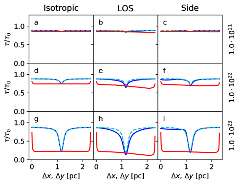
Figure 32: Ratio of estimated and true optical depths in case of simulated FIR observations of dust emission. The rows correspond different filament column densities. The columns correspond to different cases of the radiation field, with isotropic illumination or, alternatively, also including a point source at $\Delta y=2.09$ pc and at a distance of 0.93 pc from the filament centre, either along the line of sight towards the filament or to the left of the filament ($\Delta x$=-0.93 pc). The ratios are plotted along the filament centre line (red curves, as a function of $\Delta y$) or across the filament at $\Delta y=1.4$ pc (blue line) or $\Delta y=0.7$ pc (dashed cyan line).

Results on MIR dust emission were shown in Sect. 4.2.2. Similar to Fig. 15, we include below figures for the other radiation field configurations. Figure 33 shows parameter estimates along a $N({\rm H}_{2})=3\cdot 10^{23}$ cm^-2 filament that is illuminated by an isotropic radiation field with $\chi=1$. In Figs. 34 and 35, the model also includes the 590 $L_{\sun}$ radiation source that is located 0.94 pc in front of or behind the filament.

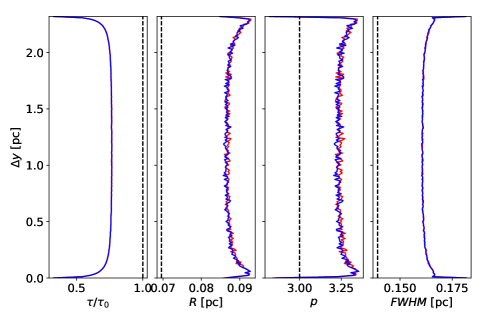
Figure 33: As Fig. 15, but showing the effect of dust emission on the MIR filament parameters in the case of an isotropic external radiation field only ($\chi$=1). The simulated surface brightness is assumed to consist of extincted background radiation and thermal emission from stochastically heated grains.

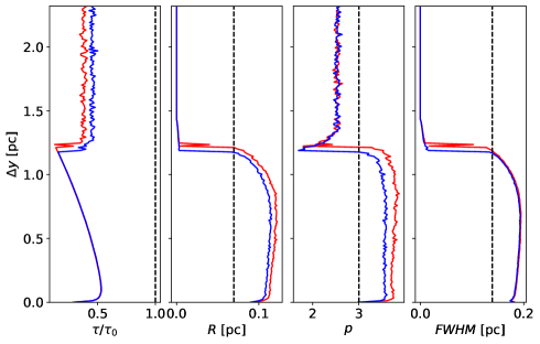
Figure 34: As Fig. 33 but with the point source located 0.93 pc in front of the model filament. Because of thermal emission from stochastically heated grains, the filament is not visible as an MIR absorption feature at $\Delta y>1.2$ pc and the corresponding data should be ignored.

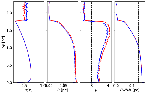
Figure 35: As Fig. 33 but with the point source located 0.93 pc behind the model filament. The filament is not visible as an absorption feature at $\Delta y>1.6$ pc, and the corresponding data should be ignored.

Figures 36-39 show the results for a less massive filament. The filament has $N({\rm H}_{2})=3\cdot 10^{22}$ cm^-2 but the assumed background sky brightness is higher, 100 MJy sr^-1.

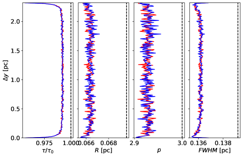
Figure 36: As Fig. 15 but for the case of lower column density $N({\rm H}_{2})=3\cdot 10^{22}$ cm^-2, higher background surface brightness $I^{\rm bg}$=100 MJy sr^-1, and the model filament illumination by an isotropic radiation field only ($\chi$=1). The observed surface brightness is assumed to consist only of the extincted background and thermal dust emission from stochastically heated grains.

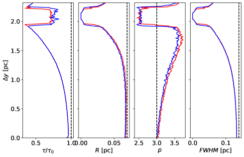
Figure 37: As Fig. 36 but including a point source at $\Delta y=2.09$ pc and 0.93 pc in front of the model filament. Around $\Delta y\approx 2-2.2$ pc, the filament is not seen in absorption because of thermal emission from stochastically heated grains.

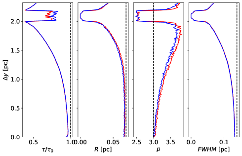
Figure 38: As Fig. 36 but including a point source at $\Delta y=2.09$ pc and 0.93 pc behind the model filament. Around $\Delta y\approx 2-2.2$ pc, the filament is not seen in absorption because of thermal emission from stochastically heated grains.

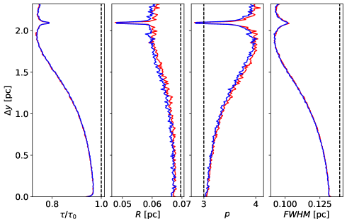
Figure 39: As Fig. 36 but including a point source at $\Delta y=2.09$ pc and 0.93 pc to one side of the model filament.

Appendix G Toy model of a filament with two temperature components

Figure 40 show toy models of a core and a filament, both with a Gaussian optical depth profile with $FWHM(\tau)=20\arcsec$. If the dust properties and especially the dust temperature were constant, one could precisely recover the expected convolved optical depth profiles with $FWHM=\sqrt{FWHM(\tau)^{2}+FWHM({\rm beam})^{2}}$, where we now assume $FWHM({\rm beam})=20\arcsec$ and $40\arcsec$ for the HR and LR maps, respectively.

The model of Fig. 40 consists however of two dust components at 10 K and 20 K temperatures. The fractional abundance of one component increases proportionally to $\tau$, and the abundance of the other component decreases, keeping their sum equal to $\tau$. Thus, at the distance from the filament centre where the optical depth has dropped to half of its maximum value, the optical depths of the warm and cold components are equal. Both methods (HR and LR) now give biased estimates of the filament width. If the filament centre is colder, the filament width is overestimated, and if the centre is warmer, the width is underestimated. The relative errors are larger for HR maps and, unlike in the isothermal cases, the errors are not identical in spherical and cylindrical geometries. In the filament case of Fig. 40b, the relative errors are +29% and -10% for the HR map and -3% and +5% for the LR map. After deconvolution the estimated width of a filament with a cold centre is 30.6$\arcsec$ based on the HR map and 24.8$\arcsec$ based on the LR map. Relative differences are larger for the HR map, which results in deconvolved sizes of 30.6$\arcsec$ and 15.8$\arcsec$ for the cold-core and the hot-core filaments, respectively. Quantitatively, the errors depend on the average temperature, the temperature contrast, and steepness and radial location of the temperature change. The above example with 20 K versus 10 K components may exaggerate the typical effects, but nevertheless suggests that the errors can be significant.

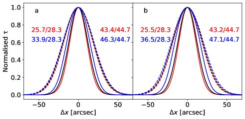
Figure 40: Optical-depth profiles of toy models consisting of 10 K and 20 K dust. The model in the left frame is a Gaussian sphere, and the model on the right a cylinder with the same Gaussian cross-section with $FWHM=20\arcsec$. The black curves are the expected profiles observed at 20$\arcsec$ and 40$\arcsec$ resolution. The actually profiles (from HR and LR maps) are plotted in red (models with warm centre) and blue (models with cold centre), where solid lines show the HR and the dashed lines the LR results. The estimated and expected FWHM values are quoted in the same colours (HR on left, and LR on right side).

References

- André et al. (2010) André, P., Men’shchikov, A., Bontemps, S., et al. 2010, A&A, 518, L102
- Aniano et al. (2011) Aniano, G., Draine, B. T., Gordon, K. D., & Sandstrom, K. 2011, PASP, 123, 1218
- Arzoumanian et al. (2011) Arzoumanian, D., André, P., Didelon, P., et al. 2011, A&A, 529, L6+
- Arzoumanian et al. (2019) Arzoumanian, D., André, P., Könyves, V., et al. 2019, A&A, 621, A42
- Bracco et al. (2017) Bracco, A., Palmeirim, P., André, P., et al. 2017, A&A, 604, A52
- Butler & Tan (2012) Butler, M. J. & Tan, J. C. 2012, ApJ, 754, 5
- Compiègne et al. (2011) Compiègne, M., Verstraete, L., Jones, A., et al. 2011, A&A, 525, A103+
- Draine (2003) Draine, B. T. 2003, ARA&A, 41, 241
- Fischera & Martin (2012) Fischera, J. & Martin, P. G. 2012, A&A, 542, A77
- Furlan et al. (2016) Furlan, E., Fischer, W. J., Ali, B., et al. 2016, ApJS, 224, 5
- Getman et al. (2019) Getman, K. V., Feigelson, E. D., Kuhn, M. A., & Garmire, G. P. 2019, MNRAS, 487, 2977
- Goicoechea et al. (2020) Goicoechea, J. R., Pabst, C. H. M., Kabanovic, S., et al. 2020, A&A, 639, A1
- Großschedl et al. (2018) Großschedl, J. E., Alves, J., Meingast, S., et al. 2018, A&A, 619, A106
- Güsten et al. (2006) Güsten, R., Nyman, L. Å., Schilke, P. andMenten, K., Cesarsky, C., & Booth, R. 2006, A&A, 454, L13
- Hacar et al. (2022) Hacar, A., Clark, S., Heitsch, F., et al. 2022, arXiv e-prints, arXiv:2203.09562
- Hacar et al. (2018) Hacar, A., Tafalla, M., Forbrich, J., et al. 2018, A&A, 610, A77
- Hennemann et al. (2012) Hennemann, M., Motte, F., Schneider, N., et al. 2012, A&A, 543, L3
- Howard et al. (2021) Howard, A. D. P., Whitworth, A. P., Griffin, M. J., Marsh, K. A., & Smith, M. W. L. 2021, MNRAS, 504, 6157
- Howard et al. (2019) Howard, A. D. P., Whitworth, A. P., Marsh, K. A., et al. 2019, MNRAS, 489, 962
- Jones et al. (2013) Jones, A. P., Fanciullo, L., Köhler, M., et al. 2013, A&A, 558, A62
- Jones et al. (2016) Jones, A. P., Köhler, M., Ysard, N., et al. 2016, A&A, 588, A43
- Juvela (2019) Juvela, M. 2019, A&A, 622, A79
- Juvela et al. (2015a) Juvela, M., Demyk, K., Doi, Y., et al. 2015a, A&A, 584, A94
- Juvela et al. (2012a) Juvela, M., Malinen, J., & Lunttila, T. 2012a, A&A, 544, A141
- Juvela et al. (2020) Juvela, M., Neha, S., Mannfors, E., et al. 2020, A&A, 643, A132
- Juvela et al. (2012b) Juvela, M., Pelkonen, V. M., White, G. J., et al. 2012b, A&A, 544, A14
- Juvela et al. (2015b) Juvela, M., Ristorcelli, I., Marshall, D. J., et al. 2015b, A&A, 584, A93
- Juvela et al. (2012c) Juvela, M., Ristorcelli, I., Pagani, L., et al. 2012c, A&A, 541, A12
- Juvela & Ysard (2012) Juvela, M. & Ysard, N. 2012, A&A, 539, A71
- Kainulainen et al. (2017) Kainulainen, J., Stutz, A. M., Stanke, T., et al. 2017, A&A, 600, A141
- Kainulainen & Tan (2013) Kainulainen, J. & Tan, J. C. 2013, A&A, 549, A53
- Kashiwagi & Tomisaka (2021) Kashiwagi, R. & Tomisaka, K. 2021, ApJ, 911, 106
- Köhler et al. (2015) Köhler, M., Ysard, N., & Jones, A. P. 2015, A&A, 579, A15
- Kong et al. (2018) Kong, S., Arce, H. G., Feddersen, J. R., et al. 2018, ApJS, 236, 25
- Könyves et al. (2015) Könyves, V., André, P., Men’shchikov, A., et al. 2015, A&A, 584, A91
- Lefèvre et al. (2014) Lefèvre, C., Pagani, L., Juvela, M., et al. 2014, A&A, 572, A20
- Lefèvre et al. (2016) Lefèvre, C., Pagani, L., Min, M., Poteet, C., & Whittet, D. 2016, A&A, 585, L4
- Li et al. (2022) Li, P. S., Lopez-Rodriguez, E., Soam, A., & Klein, R. I. 2022, MNRAS, 514, 3024
- Lombardi et al. (2014) Lombardi, M., Bouy, H., Alves, J., & Lada, C. J. 2014, A&A, 566, A45
- Lowe et al. (2022) Lowe, I., Mason, B., Bhandarkar, T., et al. 2022, ApJ, 929, 102
- Malinen et al. (2011) Malinen, J., Juvela, M., Collins, D. C., Lunttila, T., & Padoan, P. 2011, A&A, 530, A101+
- Malinen et al. (2013) Malinen, J., Juvela, M., Pelkonen, V.-M., & Rawlings, M. G. 2013, A&A, 558, A44
- Mannfors et al. (2022) Mannfors, E., Juvela, M., & et al. 2022, in preparation
- Marsh et al. (2015) Marsh, K. A., Whitworth, A. P., & Lomax, O. 2015, MNRAS, 454, 4282
- Mathis et al. (1983) Mathis, J. S., Mezger, P. G., & Panagia, N. 1983, A&A, 128, 212
- Megeath et al. (2022) Megeath, S. T., Gutermuth, R. A., & Kounkel, M. A. 2022, PASP, 134, 042001
- Men’shchikov (2013) Men’shchikov, A. 2013, A&A, 560, A63
- Ormel et al. (2011) Ormel, C. W., Min, M., Tielens, A. G. G. M., Dominik, C., & Paszun, D. 2011, A&A, 532, A43
- Ossenkopf & Henning (1994) Ossenkopf, V. & Henning, T. 1994, A&A, 291, 943
- Ostriker (1964) Ostriker, J. 1964, ApJ, 140, 1056
- Pagani et al. (2010) Pagani, L., Steinacker, J., Bacmann, A., Stutz, A., & Henning, T. 2010, Science, 329, 1622
- Palmeirim et al. (2013) Palmeirim, P., André, P., Kirk, J., et al. 2013, A&A, 550, A38
- Panopoulou et al. (2022) Panopoulou, G. V., Clark, S. E., Hacar, A., et al. 2022, A&A, 657, L13
- Pattle et al. (2017) Pattle, K., Ward-Thompson, D., Kirk, J. M., et al. 2017, MNRAS, 464, 4255
- Pilbratt et al. (2010) Pilbratt, G. L., Riedinger, J. R., Passvogel, T., et al. 2010, A&A, 518, L1
- Polychroni et al. (2013) Polychroni, D., Schisano, E., Elia, D., et al. 2013, ApJ, 777, L33
- Revéret et al. (2014) Revéret, V., André, P., Le Pennec, J., et al. 2014, in Society of Photo-Optical Instrumentation Engineers (SPIE) Conference Series, Vol. 9153, Millimeter, Submillimeter, and Far-Infrared Detectors and Instrumentation for Astronomy VII, ed. W. S. Holland & J. Zmuidzinas, 915305
- Rivera-Ingraham et al. (2016) Rivera-Ingraham, A., Ristorcelli, I., Juvela, M., et al. 2016, A&A, 591, A90
- Roy et al. (2014) Roy, A., André, P., Palmeirim, P., et al. 2014, A&A, 562, A138
- Roy et al. (2013) Roy, A., Martin, P. G., Polychroni, D., et al. 2013, ApJ, 763, 55
- Sadavoy et al. (2016) Sadavoy, S. I., Stutz, A. M., Schnee, S., et al. 2016, A&A, 588, A30
- Salas et al. (2021) Salas, P., Rugel, M. R., Emig, K. L., et al. 2021, A&A, 653, A102
- Schmiedeke et al. (2021) Schmiedeke, A., Pineda, J. E., Caselli, P., et al. 2021, ApJ, 909, 60
- Schnee et al. (2014) Schnee, S., Mason, B., Di Francesco, J., et al. 2014, MNRAS, 444, 2303
- Schuller et al. (2021) Schuller, F., André, P., Shimajiri, Y., et al. 2021, A&A, 651, A36
- Shetty et al. (2009) Shetty, R., Kauffmann, J., Schnee, S., Goodman, A. A., & Ercolano, B. 2009, ApJ, 696, 2234
- Sousbie (2011) Sousbie, T. 2011, MNRAS, 414, 350
- Steinacker et al. (2014a) Steinacker, J., Andersen, M., Thi, W.-F., & Bacmann, A. 2014a, A&A, 563, A106
- Steinacker et al. (2014b) Steinacker, J., Ormel, C. W., Andersen, M., & Bacmann, A. 2014b, A&A, 564, A96
- Steinacker et al. (2010) Steinacker, J., Pagani, L., Bacmann, A., & Guieu, S. 2010, A&A, 511, A9+
- Stodólkiewicz (1963) Stodólkiewicz, J. S. 1963, Acta Astron., 13, 30
- Stutz & Kainulainen (2015) Stutz, A. M. & Kainulainen, J. 2015, A&A, 577, L6
- Suri et al. (2019) Suri, S., Sánchez-Monge, Á., Schilke, P., et al. 2019, A&A, 623, A142
- Tanabe et al. (2019) Tanabe, Y., Nakamura, F., Tsukagoshi, T., et al. 2019, PASJ, 71, S8
- Werner et al. (2004) Werner, M. W., Roellig, T. L., Low, F. J., et al. 2004, ApJS, 154, 1