Enhancing Deep Traffic Forecasting Models with Dynamic Regression

Abstract

A common assumption in deep learning-based multivariate and multistep traffic time series forecasting models is that residuals are independent, isotropic, and uncorrelated in space and time. While this assumption provides a straightforward loss function (such as MAE/MSE), it is inevitable that residual processes will exhibit strong autocorrelation and structured spatiotemporal correlation. In this paper, we propose a complementary dynamic regression (DR) framework to enhance existing deep multistep traffic forecasting frameworks through structured specifications and learning for the residual process. Specifically, we assume the residuals of the base model (i.e., a well-developed traffic forecasting model) are governed by a matrix-variate seasonal autoregressive (AR) model, which can be seamlessly integrated into the training process by redesigning the overall loss function. Parameters in the DR framework can be jointly learned with the base model. We evaluate the effectiveness of the proposed framework in enhancing several state-of-the-art deep traffic forecasting models on both speed and flow datasets. Our experiment results show that the DR framework not only improves existing traffic forecasting models but also offers interpretable regression coefficients and spatiotemporal covariance matrices.

1 Introduction

Traffic forecasting is a fundamental task in intelligent transportation systems (ITS), with diverse applications such as trip planning, route planning, travel time estimation, and traffic flow management, to name a few Vlahogianni et al. (2014). Essentially, the traffic forecasting task can be formulated as a multivariate and multistep time series forecasting problem. Suppose there are $N$ sensors in a traffic network, the collected traffic data can be stored in the form of a tensor with shape $N\times T$ over an observation period $T$. The goal of traffic forecasting is to predict the traffic states of $Q$ future steps given the most recent $P$ historical steps.

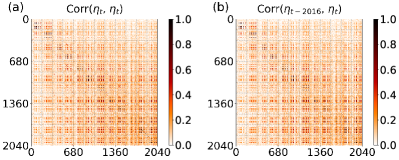
Figure 1: Correlation matrices of the residuals obtained from STSGCN on PEMS08, where $\bm{\eta}_{t}=\operatorname{vec}(\bm{R}_{t})\in\mathbb{R}^{NQ}$ is the vectorized residual matrix at time $t$ ($N=170$ and $Q=12$). (a) Spatial and across-step correlation. (b) Autocorrelation for lag-2016 (i.e., one week).

Deep learning (DL) models have gained widespread use in traffic forecasting in recent years, and have shown exceptional performance due to their ability to model and capture the nonlinearity and spatiotemporal structures in traffic data. Many powerful multistep forecasting models have been developed, such as STGCN Yu et al. (2018), DCRNN Li et al. (2018), Graph Wavenet Wu et al. (2019), and STSGCN Song et al. (2020). These DL models are typically trained using mean absolute error (MAE) or mean squared error (MSE) based on the $N\times Q$ residual term, under the assumption that: (i) the residuals at different time points are independent with no temporal correlation, and (ii) entries in the $N\times Q$ residual matrix are independent and isotropic, with no concurrent correlations. However, these assumptions do not hold true for real-world datasets. On the one hand, due to the exclusion of important/relevant features, we will expect the residual process to be autocorrelated in time. For example, when forecasting traffic speed, DL models often ignore important time-varying factors such as weather conditions and vehicle flow rates, leading to temporally correlated residuals. On the other hand, as our target multistep-ahead forecasting, we would expect there exist certain spatiotemporal correlations in the residual process, rather than assuming that its entries are independent and isotropic. A simple example is that we definitely expect the prediction variance at 60-min-ahead to be much larger than that of 5-min-ahead. Ignoring these factors may negatively impact the performance of DL models. For example, in Figure 1, we present the spatial and across-step correlation $\operatorname{Corr}(\bm{\eta}_{t},\bm{\eta}_{t})$ and the lag-2016 autocorrelation $\operatorname{Corr}(\bm{\eta}_{t-2016},\bm{\eta}_{t})$ based on the residuals obtained from learning STSGCN Song et al. (2020) on the PEMS08 traffic flow dataset with MAE loss. As we can see, both correlation matrices exhibit clear spatiotemporal structures. In particular, we posit that the substantial autocorrelation in $\operatorname{Corr}(\bm{\eta}_{t-2016},\bm{\eta}_{t})$ is mainly caused by overlooking time of week, trip purpose distribution, and traffic congestion information as significant covariates that have a dominating effect on observed flow. In this case, it might be tempting to include additional relevant covariates in the DL-based traffic flow forecasting model; however, this would introduce a very large set of covariates that makes it difficult to train the DL model, not to mention that these covariates are always available. The statistical characteristics of the residual process provide opportunities for enhancing these DL models.

In this study, we propose a straightforward yet effective method for adjusting spatiotemporal residual correlation using a dynamic regression (DR) framework, which can be applied to any DL model for traffic forecasting. We assume the residual of the base model follows a matrix-variate autoregressive (AR) process that can be integrated into the original DL model. In addition to learning the AR coefficient, we also effectively learn the concurrent covariance matrix for the error, which is assumed to follow a matrix normal distribution. The parameters of the residual regression module and the error covariance matrices are jointly optimized with the parameters of the base model (i.e., a selected DL model). The main contributions of this work are as follows:

• We propose a bi-linear autoregressive form for the matrix-valued residual to address the autocorrelation problem. The regression coefficient matrices are interpretable in a way that we can uncover how the current residual is related to the past residual.

• We explicitly model the error term in the matrix-variate AR model with a matrix normal distribution. The negative log-likelihood of this distribution is incorporated into the loss function to facilitate joint optimization. The obtained covariance matrices are interpretable and can be further used to perform probabilistic forecasting with uncertainty quantification.

• We evaluate our proposed method on a variety of traffic datasets and achieve universal improvement on many state-of-the-art DL-based traffic forecasting models.

2 Related Works

2.1 Deep Learning for Traffic Forecasting

Here, we review some signature frameworks for DL-based multivariate and multistep traffic forecasting models. Starting from the DCRNN framework Li et al. (2018), modern deep learning models are generally featured with a combination of different neural networks to process the spatial and temporal dependencies in traffic data. For example, DCRNN uses a diffusion convolution operation to model the spatial dependency. The convolution process is integrated into Gated Recurrent Units (GRUs) for modeling temporal dependency. The STGCN framework Yu et al. (2018) uses Graph Convolutional Networks (GCNs) to extract spatial correlations and Convolutional Neural Networks (CNNs) to extract temporal correlations. GCNs have the advantage of incorporating graph structure into the spatial modeling process. CNNs can reduce the training time through parallel computing since it avoids the recurrent process in Recurrent Neural Networks (RNNs). Building on STGCN, the ASTGCN framework Guo et al. (2019) integrates a spatiotemporal attention mechanism to pre-process the traffic data before being fed to the convolutional layers. Both STGCN and ASTGCN use a pre-calibrated adjacency matrix that cannot be jointly learned with the model. The Graph WaveNet framework Wu et al. (2019) uses an adaptive adjacency matrix to learn the graph structure. The entries in the adjacency matrix are treated as trainable parameters in the optimization. Dilated causal convolution is used as Temporal Convolutional Networks (TCNs) to model temporal dependency and GCNs are used to model spatial dependency. Prior GCN-based architectures process spatial information and temporal information separately. Song et al. proposed the STSGCN framework Song et al. (2020) to learn spatial and temporal information simultaneously by connecting individual spatial graphs of adjacent time steps into one graph. STSGCN has shown superior performance to the previous GCN-based frameworks. Other state-of-the-art models include GMAN Zheng et al. (2020), N-BEATS Oreshkin et al. (2020), and FC-GAGA Oreshkin et al. (2021), to name a few.

2.2 Adjusting for Correlated Residuals

The detection and adjustment for autocorrelated residuals in time series data has been studied extensively in econometrics using models with exact forms Durbin and Watson (1950); Ljung and Box (1978); Breusch (1978); Godfrey (1978); Cochrane and Orcutt (1949); Prais and Winsten (1954); Beach and MacKinnon (1978). With the rapid advances in DL-based forecasting models, how to learn and adjust for the residual process in DL-based time series models has attracted significant attention in recent studies. There are essentially two statistical approaches to modeling the residual process: (i) capturing autocorrelation and (ii) learning concurrent correlation in independent errors. For correcting autocorrelation, Sun et al. (2021) proposed a reparametrization approach of the input and the output of a neural network for time series forecasting. The reparametrization approach is inherently considered a first-order residual AR process using a linear regression form. The method successfully enhanced performance for many DL-based one-step-ahead forecasting models on a wide range of time series datasets and facilitated joint optimization of parameters of the base regressor and the residual regressor. Kim et al. (2022) designed a light deep learning module to calibrate residual autocorrelation on the predictions of pre-trained traffic forecasting models. The calibration module takes recently observed residuals and predictions as input to predict future residuals. The method can improve the performance of many traffic forecasting models on traffic speed datasets. In terms of learning error covariance, Jia and Benson (2020) suggested that there is no reason to assume independence in the residuals of a node regression problem. The authors proposed to model the residual correlation using a multivariate Gaussian distribution. Thus the prediction of unknown nodes can be adjusted based on those known node labels. The method was also referred to as the residual propagation in Graph Neural Networks (GNNs). Using a similar idea but in a classification task, Huang et al. (2020) proposed a correct-and-smooth model as a post-processing scheme to correct for the correlated residuals in GNNs. Choi et al. (2022) proposed a dynamic mixture of matrix normal Gaussian to regularize the spatiotemporal correlation of residuals.

However, these methods either take a post-hoc calibration approach or a reparametrization approach, which may not be directly applicable to traffic forecasting, as it involves a multivariate sequence-to-sequence (seq2seq) problem with strong seasonality. The key challenge is that the residual process becomes an $N\times Q$ matrix-variate time series with prominent temporal dynamics and structured error covariance structure, which need to be jointly learned with the base DL model.

3 Methodology

In this section, we will introduce the general formulation of a multistep traffic forecasting problem, as well as the dynamic regression framework to characterize residual autocorrelation.

3.1 Traffic Forecasting

A traffic network can be defined as a directed graph $\mathcal{G}=\left(\mathcal{V},\mathcal{E},\bm{W}\right)$, where $\mathcal{V}$ with $|\mathcal{V}|=N$ is a set of nodes representing traffic sensors; $\mathcal{E}$ is a set of links connecting these nodes; $\bm{W}\in\mathbb{R}^{N\times N}$ is a weighted adjacency matrix characterizing the proximity of nodes. Denote by $\bm{z}_{t}\in\mathbb{R}^{N}$ the vector of observed traffic states at time $t$. The traffic forecasting problem aims to learn a function that maps data from $P$ past steps to the prediction of $Q$ future steps. Denote by $\bm{X}_{t}=\left[\bm{z}_{t-P+1},\dots,\bm{z}_{t}\right]\in\mathbb{R}^{P\times N}$ and $\bm{Y}_{t}=\left[\bm{z}_{t+1},\dots,\bm{z}_{t+Q}\right]\in\mathbb{R}^{Q\times N}$, we have

$${\bm{Y}}_{t}=f_{\theta}(\bm{X}_{t},\bm{W})+\bm{R}_{t},$$ (1)

where $f_{\theta}(\bm{X}_{t},\bm{W})$ is a seq2seq deep learning model that generates the predicted mean and $\bm{R}_{t}\in\mathbb{R}^{N\times Q}$ is a zero-mean residual process. In many cases, a seq2seq model $f$ is trained with MSE as the loss function:

$$\mathcal{L}=\sum_{t}\|\bm{R}_{t}\|_{F}^{2}=\sum_{t}\|\bm{Y}_{t}-f_{\theta}(\bm{X}_{t},\bm{W})\|_{F}^{2}.$$ (2)

This loss function simply assumes: (i) $\bm{R}_{t}$ is temporally independent, i.e., there is no correlation between $\bm{R}_{s}$ and $\bm{R}_{t}$ when $s\neq t$; and (ii) entries in $\bm{R}_{t}$ follow an isotropic Gaussian with no concurrent correlations, i.e., $\bm{\eta}_{t}=\operatorname{vec}(\bm{R}_{t})\sim\mathcal{N}(\bm{0},\sigma^{2}\bm{I}_{NQ})$. Likewise, using MAE as the loss function corresponds to assuming entries in $\bm{R}_{t}$ follow a Laplacian distribution.

3.2 Modeling Residual with Matrix-valued Autoregression

Following the idea of dynamic regression Hyndman and Athanasopoulos (2018), we assume that the relationship between the input $\bm{X}_{t}$ and the output $\bm{Y}_{t}$ has been fully captured by the seq2seq model $f_{\theta}(\cdot)$, and the unexplained residual $\bm{R}_{t}$ is governed by a temporal process. For example, for a one-step-ahead prediction model (i.e., $\bm{\eta}_{t}=\bm{R}_{t}$ as $Q=1$), it is straightforward to model $\bm{\eta}_{t}$ using a $p$-th order vector autoregressive model:

$$\bm{\eta}_{t}=\bm{C}_{1}\bm{\eta}_{t-1}+\ldots+\bm{C}_{p}\bm{\eta}_{t-p}+\bm{\epsilon}_{t},$$ (3)

where $C_{l}\in\mathbb{R}^{N\times N}$ ($l=1,\ldots,p$) are the regression coefficient, and $\bm{\epsilon}_{t}\sim\mathcal{N}\left(0,\bm{\Sigma}\right)$ is an independent white-noise process.

However, for a seq2seq prediction model with $Q>1$, the $N\times Q$ error $\bm{R}_{t}$ at time $t$ cannot be directly modeled using Eq. (3), as the residuals, $\{\bm{R}_{t-l}\,|\,l=1,\ldots,Q-1\}$, will not be accessible. To address this issue, we instead try to model the relation between $\bm{R}_{t}$ and those lagged residuals that are accessible, i.e., $\bm{R}_{t-\Delta_{l}}$ for $l=1,\ldots,p$ as long as $\Delta_{l}\geq Q$. Therefore, we have the model for the vector $\bm{\eta}_{t}$ as:

$$\bm{\eta}_{t}=\bm{C}_{1}\bm{\eta}_{t-\Delta_{1}}+\ldots+\bm{C}_{p}\bm{\eta}_{t-\Delta_{p}}+\bm{\epsilon}_{t},$$ (4)

where $\bm{C}_{l}\in\mathbb{R}^{NQ\times NQ}$ and the size of the white-noise covariance matrix $\bm{\Sigma}$ is also of size $NQ\times NQ$. As traffic data often shows strong day-to-day and week-to-week similarity, for simplicity we only introduce one lagged residual component $\bm{R}_{t-\Delta}$, where $\Delta$ is pre-selected seasonal lag (e.g., one day, one week) with strong correlations with the current time.

Still, a clear limitation of the above formulation is that it introduces too many parameters in $\bm{C}$ and $\bm{\Sigma}$. To further simplify the temporal process, we assume the $\bm{R}_{t}$ follows a bi-linear autoregressive model Chen et al. (2021); Hsu et al. (2021):

$$\bm{R}_{t}=\bm{A}\bm{R}_{t-\Delta}\bm{B}+\bm{E}_{t},$$ (5)

where $\bm{A}\in\mathbb{R}^{N\times N}$ and $\bm{B}\in\mathbb{R}^{Q\times Q}$ are regression coefficients, and $\bm{E}_{t}$ follows an independent matrix white-noise process. The vectorized version of Eq. (5) becomes

$$\bm{\eta}_{t}=(\bm{B}^{\top}\otimes\bm{A})\bm{\eta}_{t-\Delta}+\bm{\epsilon}_{t},$$ (6)

and we can see that the bi-linear formulation is equivalent to imposing a Kronecker product structure on the coefficient matrix $\bm{C}=\bm{B^{\top}}\otimes\bm{A}$ in Eq. (4), and thus it substantially reduces the number of parameters. Combining Eqs. (1) and (5), we can build a better loss function, such as MAE, on $\bm{E}_{t}$ instead of $\bm{R}_{t}$:

$$\bm{E}_{t}=\bm{Y}_{t}-f_{\theta}(\bm{X}_{t})-\bm{A}\left(\bm{Y}_{t-\Delta}-f_{\theta}(\bm{X}_{t-\Delta})\right)\bm{B},$$ (7)

$$\mathcal{L}_{\text{mae}}=\sum_{t}\|\bm{E}_{t}\|_{1},$$ (8)

where $\bm{A}$ and $\bm{B}$, as trainable parameters, can be jointly updated with the base regressor $f_{\theta}(\cdot)$. When $\bm{R}_{t}$ and $\bm{R}_{t-\Delta}$ have no relations (e.g., when $\bm{A}=\bm{0}$), $\mathcal{L}_{\text{mae}}$ collapse to the default MAE loss used in existing DL models. If both $\bm{A}$ and $\bm{B}$ are identity matrices, the model corresponds to assuming the residual process follows a seasonal random walk. Here we consider both $\bm{A}$ and $\bm{B}$ as trainable parameters for flexibility and interpretability. To promote sparsity in $\bm{A}$ and $\bm{B}$, we also introduce an $l1$ regularization term into the loss function:

$$\mathcal{L}_{\text{res}}=\frac{1}{N^{2}}\|\bm{A}\|_{1}+\frac{1}{Q^{2}}\|\bm{B}\|_{1}.$$ (9)

Once the base model $f_{\theta}()$ and coefficients $\bm{A}$ and $\bm{B}$ are learned, prediction at time $t$ can be made by:

$$\hat{\bm{Y}}_{t}=f_{\theta}(\bm{X}_{t})+\bm{A}\left(\bm{Y}_{t-\Delta}-f_{\theta}(\bm{X}_{t-\Delta})\right)\bm{B}.$$ (10)

3.3 Spatiotemporal Covariance Structure for the Matrix White Noise

We next try to consider the concurrent spatiotemporal correlation among entries in the white noise $\bm{E}_{t}$ through learning its covariance matrix $\bm{\Sigma}$. The key challenge here is the size (i.e., $NQ\times NQ$) of $\bm{\Sigma}$. For model scalability, we follow Choi et al. (2022) and assume $\bm{E}_{t}$ to follow a zero-mean matrix normal distribution $\bm{E}_{t}\sim\mathcal{MN}(\bm{0},\bm{\Sigma}_{N},\bm{\Sigma}_{Q})$ with

$$p\left(\bm{E}_{t}\right)=\frac{\exp{\left(-\frac{1}{2}\operatorname{tr}\left(\bm{\Sigma}_{Q}^{-1}\bm{E}_{t}^{\top}\bm{\Sigma}_{N}^{-1}\bm{E}_{t}\right)\right)}}{(2\pi)^{\frac{NQ}{2}}|\bm{\Sigma}_{Q}|^{\frac{N}{2}}|\bm{\Sigma}_{N}|^{\frac{Q}{2}}},$$ (11)

where $\bm{\Sigma}_{N}$ and $\bm{\Sigma}_{Q}$ are covariance matrices of the matrix normal distribution capturing the correlation across forecasting steps and spatial locations. The negative log-likelihood of this distribution is included in the loss function to facilitate joint optimization:

$$\mathcal{L}_{\text{nll}} =-\log p(\bm{E}_{t}\,|\,\bm{0},\bm{\Sigma}_{N},\bm{\Sigma}_{Q})$$ (12)

$$=\frac{NQ}{2}\log(2\pi)+\frac{Q}{2}\log|\bm{\Sigma}_{N}|+\frac{N}{2}\log|\bm{\Sigma}_{Q}|$$

$$+\frac{1}{2}\operatorname{tr}\left(\bm{\Sigma}_{Q}^{-1}\bm{E}_{t}^{\top}\bm{\Sigma}_{N}^{-1}\bm{E}_{t}\right).$$

As we have to calculate the inverse and determinant of $\bm{\Sigma}_{N}$, $\bm{\Sigma}_{Q}$, we parameterize the precision matrix (i.e., the inverse of the covariance matrix) directly to avoid numerical problems and consider the Cholesky decomposition of the precision matrix as trainable parameters following Choi et al. (2022):

$$\begin{split}&\bm{\Lambda}_{N}=\bm{\Sigma}_{N}^{-1},\ \ \bm{\Lambda}_{Q}=\bm{\Sigma}_{Q}^{-1},\\ &\bm{\Lambda}_{N}=\bm{L}_{N}\bm{L}_{N}^{\top},\ \ \bm{\Lambda}_{Q}=\bm{L}_{Q}\bm{L}_{Q}^{\top},\end{split}$$ (13)

where $\bm{L}_{N}\in\mathbb{R}^{N\times N}$ and $\bm{L}_{Q}\in\mathbb{R}^{Q\times Q}$ are lower-triangular Cholesky factors (as trainable parameters) that can be jointly optimized with other model parameters. The determinant can be conveniently calculated by summing the logarithm of diagonal entries of the lower triangular Cholesky factors:

$$\begin{split}\log|\bm{\Sigma}_{N}|&=-\log|\bm{\Lambda}_{N}|=-2\sum_{n=1}^{N}\log[\bm{L}_{N}]_{n,n},\\ \log|\bm{\Sigma}_{Q}|&=-\log|\bm{\Lambda}_{Q}|=-2\sum_{q=1}^{Q}\log[\bm{L}_{Q}]_{q,q}.\\ \end{split}$$ (14)

In addition, the trace can be simplified into

$$\operatorname{tr}\left(\bm{\Lambda}_{Q}\bm{E}_{t}^{\top}\bm{\Lambda}_{N}\bm{E}_{t}\right) =\operatorname{tr}\left(\bm{L}_{Q}\bm{L}_{Q}^{\top}\bm{E}_{t}^{\top}\bm{L}_{N}\bm{L}_{N}^{\top}\bm{E}_{t}\right)$$ (15)

$$=\operatorname{tr}\left(\bm{L}_{N}^{\top}\bm{E}_{t}\bm{L}_{Q}\bm{L}_{Q}^{\top}\bm{E}_{t}^{\top}\bm{L}_{N}\right)$$

$$=\operatorname{tr}\left(\bm{K}_{t}\bm{K}_{t}^{\top}\right)=\|\bm{K}_{t}\|_{F}^{2},$$

where $\bm{K}_{t}=\bm{L}_{N}^{\top}\bm{E}_{t}\bm{L}_{Q}$. Substitute Eq. (14) and Eq. (15) into Eq. (12), we obtain a probabilistic loss function to learn the correlation structure in $\bm{E}_{t}$:

$$\mathcal{L}_{\text{nll}}=\frac{1}{2}\|\bm{K}_{t}\|_{F}^{2}-Q\sum_{n=1}^{N}\log[\bm{L}_{N}]_{n,n}-N\sum_{q=1}^{Q}\log[\bm{L}_{Q}]_{q,q}.$$ (16)

As the covariance matrix determines the spatial and across-step correlations in $\bm{E}_{t}$, we posit that it will not only improve model accuracy but also provide better uncertainty quantification when performing probabilistic forecasting.

4 Experiments

To evaluate the effectiveness of the proposed method, we conduct experiments on three traffic datasets: PEMSD7 (M), PEMS03, and PEMS08. PEMSD7 (M) is a highway traffic speed dataset originally used in STGCN Yu et al. (2018). PEMS03 and PEMS08 are highway traffic flow data originally used in ASTGCN Guo et al. (2019) and STSGCN Song et al. (2020). We adopt the same data processing procedures as in the original papers. For PEMS03 and PEMS08, 60% of the data was used for training, 20% for validation, and the remaining 20% for testing. For PEMSD7 (M), the split ratio is 7:1:2. On all datasets, we apply z-score normalization with statistics obtained from the training set. The summary of datasets is provided in Table 1.

Datasets	#Nodes	#Time Steps	Resolution
PEMSD7 (M)	228	12,672	5 min
PEMS03	358	26,208	5 min
PEMS08	170	17,856	5 min

Table 1: Dataset Description

4.1 Baselines

In accordance with the datasets we select for verifying our method, we test our method with the following state-of-the-art models as the base model $f$.

• STGCN Yu et al. (2018): Spatiotemporal graph convolutional network, which uses ChebNet to process spatial correlation and CNNs to process temporal correlation.

• ASTGCN Guo et al. (2019): Attention-based spatiotemporal graph convolutional network, which attaches spatial and temporal attention mechanisms to STGCN for learning dynamic spatial-temporal correlations of traffic data.

• STSGCN Song et al. (2020): Spatial-temporal synchronous graph convolutional network that captures spatial-temporal correlations over the time axis.

• Graph WaveNet Wu et al. (2019): A spatiotemporal forecasting model that combines dilated 1D convolution for modeling temporal dynamics and graph convolution for modeling spatial dynamics.

4.2 Experimental Setups

Our experiments were conducted under a computer environment with one Intel(R) Xeon(R) CPU E5-2698 v4 @ 2.20GHz and four NVIDIA Tesla V100 GPU. We implemented the baseline models using the original source code (or their PyTorch version). All models use 12 steps of historical observations ($P=12$) to predict 12 steps of future values ($Q=12$). We trained all models using the Adam optimizer with an initial learning rate of 0.001, and a weight decay of 0.0001. Early stopping was applied to prevent over-fitting when the validation loss keeps increasing for more than 30 epochs. All presented results are based on the average of evaluation metrics from three independent runs.

For the residual AR process proposed in section 3.2, we need to determine the lag length $\Delta$ and the initialization of the regression matrices $\bm{A}$ and $\bm{B}$. Since traffic data is featured with strong local correlation and seasonality, we mainly consider the autocorrelation between the current residual and its 1) most recently available one ($\Delta=Q$); 2) one day apart one ($\Delta=\text{1 day}$); and 3) one week apart one ($\Delta=\text{1 week}$). The consideration of seasonal residual correlation is novel to previous works Sun et al. (2021); Kim et al. (2022). As for the initialization of $\bm{A}$ and $\bm{B}$, we attempt three different settings: 1) random. $\bm{A}$ and $\bm{B}$ consist of random numbers sampled from a normal distribution with mean 0 and variance 1; 2) zeros. $\bm{A}$ and $\bm{B}$ are zero matrices; 3) diagonal. $\bm{A}$ and $\bm{B}$ are diagonal matrices. The initial values of parameters in these settings are scaled down to very small numbers so that the model is nearly equivalent to the original model at the beginning of the training stage. Based on the preliminary observation of autocorrelation matrices, we used $\Delta=Q$ for PEMSD7 (M), $\Delta=\text{1 day}$ for PEMS03, and $\Delta=\text{1 week}$ for PEMS08. For the initialization, we chose “random” and “zeros” for STGCN and Graph WaveNet on PEMSD7 (M), “diagonal” for PEMS03, and “random” for PEMS08. For the parameters of the matrix normal distribution in section 3.3, the matrices $\bm{L}_{N}$ and $\bm{L}_{Q}$ consist of random numbers sampled from a normal distribution with mean 0 and variance 1. The Softplus function is applied to enforce positive diagonals of $\bm{L}_{Q}$ and $\bm{L}_{N}$.

The final loss function is composed of three parts:

$$\mathcal{L}=\mathcal{L}_{\text{mae}}+\omega\mathcal{L}_{\text{res}}+\rho\mathcal{L}_{\text{nll}},$$ (17)

where $\mathcal{L}_{\text{mae}}$ and $\mathcal{L}_{\text{res}}$ are the MAE loss built on Eq. (8) and the $l1$ regularization in Eq. (9), respectively, $\mathcal{L}_{\text{nll}}$ is the probabilistic loss term in Eq. (16), and $\omega$ and $\rho$ are weight parameters. We set $\omega=1$, and use $\rho=0.001$ for PEMSD7 (M) and PEMS03, $\rho=0.0001$ for PEMS08. The evaluation metrics are MAE and RMSE. Missing values are excluded from both training and testing.

In comparison to the base model, the proposed method introduces four additional learnable parameters, i.e., $\bm{A}\in\mathbb{R}^{N\times N}$, $\bm{B}\in\mathbb{R}^{Q\times Q}$, and two lower-triangular Cholesky factors $\bm{L}_{N}$ and $\bm{L}_{Q}$. Nevertheless, the size of additional parameters is almost negligible compared to the overall size of the base DL model.

4.3 Experimental Results

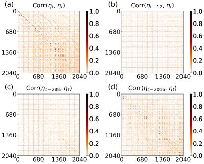
Figure 2: Correlation matrices of the residuals obtained from Graph WaveNet on PEMS08. From (a) to (b): Spatial and across-step correlation, autocorrelation for lag-12 (i.e., most recent), lag-288 (i.e., 1 day), lag-2016 (i.e., 1 week).

We begin by demonstrating that the residuals of an original traffic forecasting model are spatially and temporally correlated. We calculate two types of correlation: $\operatorname{Corr}(\bm{\eta}_{t},\bm{\eta}_{t})$ and $\operatorname{Corr}(\bm{\eta}_{t-\Delta},\bm{\eta}_{t})$. $\operatorname{Corr}(\bm{\eta}_{t},\bm{\eta}_{t})$ is the spatial and across-step correlation of the variables in $\bm{\eta_{t}}$, while $\operatorname{Corr}(\bm{\eta}_{t-\Delta},\bm{\eta}_{t})$ is the autocorrelation at lag $\Delta$. Ideally, if the residuals are independently sampled from an isotropic distribution, $\operatorname{Corr}(\bm{\eta}_{t},\bm{\eta}_{t})$ should be an identity matrix and $\operatorname{Corr}(\bm{\eta}_{t-\Delta},\bm{\eta}_{t})$ should be a zero matrix. In Figure 2, we present the residual correlation matrices of PEMS08 using the results from Graph WaveNet. We can observe that $\operatorname{Corr}(\bm{\eta}_{t},\bm{\eta}_{t})$ is not diagonal, suggesting there exists spatial and across-step correlation in the residuals. In terms of $\operatorname{Corr}(\bm{\eta}_{t-\Delta},\bm{\eta}_{t})$, we examine different values including $\Delta=12$ (1 hour), $\Delta=288$ (1 day), and $\Delta=2016$ (1 week). Interestingly, we find that $\Delta=2016$ (one week) provides the strongest correlation patterns, while correlations when $\Delta=12$ and $\Delta=288$ are weak. We believe this is mainly due to the fact that traffic flow is heavily determined by traffic demand, which often exhibits prominent weekly periodicity but is overlooked in the flow forecasting tasks. Therefore, we choose $\Delta=2016$ for the residual AR process for PEMS08.

Data	Model	1-step		3-step		6-step		12-step
		MAE	RMSE	MAE	RMSE	MAE	RMSE	MAE	RMSE
PEMSD7	STGCN (w/o our method)	2.70	5.01	3.03	5.61	3.49	6.54	4.26	8.04
	STGCN (w/ our method)	2.39	3.65	2.78	4.53	3.35	5.80	4.41	7.72
	Graph WaveNet (w/o our method)	1.29	2.20	2.12	3.97	2.74	5.37	3.33	6.58
	Graph WaveNet (w/ our method)	1.28	2.17	2.12	3.96	2.72	5.33	3.26	6.43
PEMS03	STSGCN (w/o our method)	13.49	21.93	15.54	25.44	17.63	29.00	21.73	35.26
	STSGCN (w/ our method)	13.38	21.55	15.31	24.82	17.34	28.00	21.15	33.66
	Graph WaveNet (w/o our method)	12.44	21.03	13.77	23.91	14.94	25.99	16.68	28.52
	Graph WaveNet (w/ our method)	12.25	20.56	13.54	23.22	14.67	25.35	16.42	28.03
PEMS08	STSGCN (w/o our method)	13.84	21.29	15.74	24.47	17.61	27.70	21.50	33.66
	STSGCN (w/ our method)	13.81	21.22	15.61	24.26	17.36	27.21	20.82	32.15
	ASTGCN (w/o our method)	13.97	21.21	16.12	24.60	17.95	27.38	21.57	32.50
	ASTGCN (w/ our method)	13.79	21.13	15.36	23.87	16.27	25.77	17.99	28.87
	Graph WaveNet (w/o our method)	12.81	19.95	13.92	22.17	15.04	24.29	16.74	26.80
	Graph WaveNet (w/ our method)	11.66	19.45	12.58	21.45	13.46	23.24	14.76	25.49

Table 2: Effect of the proposed method on different models and datasets.

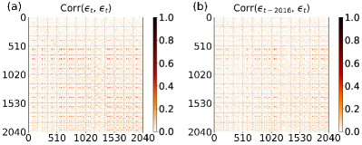
Figure 3: Correlation matrices of the residuals obtained from Graph WaveNet on PEMS08 after applying our method. (a) Spatial and across-step correlation; (b) Autocorrelation for lag-2016 (i.e., one week).

Table 2 summarizes the effectiveness of our method on a variety of DL models and datasets for 1-step, 3-step, 6-step, and 12-step ahead predictions. Models with our approach achieve superior results in almost all cases. We can observe that Graph WaveNet achieves the best performance compared with other models due to the implementation of an adaptive adjacency matrix. After implementing our method, Graph WaveNet can be further improved by a significant margin even for the 1-step ahead prediction scenario where the original models already perform very well. For example, the 1-step MAE of Graph WaveNet on PEMS08 decreases from 12.81 to 11.66, suggesting there remain explainable parts that the original model does not capture. As shown in Figure 3, both the spatial correlation and the autocorrelation for lag-2016 are greatly reduced when compared to Figure 2. For models presenting stronger residual correlations, e.g., STSGCN and ASTGCN, our approach can realize greater enhancement, especially for the 12-step ahead prediction. For example, the 12-step MAE of ASTGCN decreases from 21.57 to 17.99 on PEMS08. The various marginal improvement indicates the effectiveness of our method mainly depends on how strong the autocorrelation exists in the residuals of the original models as well as how well the assumption of matrix normal distribution can characterize the errors.

4.3.1 Ablation Study

Model	1-step		3-step		6-step		12-step
	MAE	RMSE	MAE	RMSE	MAE	RMSE	MAE	RMSE
Graph WaveNet	12.81	19.95	13.92	22.17	15.04	24.29	16.74	26.80
Our methods	11.66	19.45	12.58	21.45	13.46	23.24	14.76	25.49
Our methods w/o $\mathcal{L}_{\text{nll}}$	11.79	19.59	12.73	21.61	13.65	23.46	15.04	25.78
Our methods w/o DR	12.66	19.76	13.79	21.89	14.85	23.79	16.50	26.31

Table 3: Ablation study on PEMS08 using Graph WaveNet.

To study the effect of the two components of the proposed DR framework individually, we compare results using only the residual AR module or the error covariance learning module (Table 3). “w/o $\mathcal{L}_{\text{nll}}$” represents the model variant without adding the negative log-likelihood loss of the error to the loss function. “w/o DR” represents the model variant that uses matrix normal distribution to characterize $\bm{R}_{t}$ directly and the residual AR process is not applied. We use Graph WaveNet and PEMS08 as an example since autocorrelation $\operatorname{Corr}(\bm{\eta}_{t-\Delta},\bm{\eta}_{t})$ and spatial/across-step correlation $\operatorname{Corr}(\bm{\eta}_{t},\bm{\eta}_{t})$ are both prominent in this case (Figure 2). The results in Table 3 demonstrate that the model obtains the best performance when both components are applied. Although model variants with only one component can still outperform the original model, the results verify that the two components can act concurrently to adjust the model toward a higher accuracy. In addition, we can observe that the model benefits more from the residual AR process in this specific case since the model without $\mathcal{L}_{\text{nll}}$ is featured with higher accuracy than the model without DR.

4.3.2 Model Interpretation

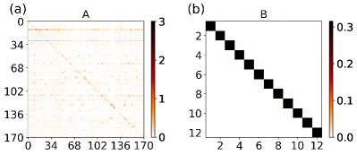
Figure 4: Learned regression coefficient matrices $\bm{A}$ and $\bm{B}$ of Graph WaveNet on PEMS08.

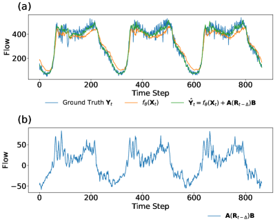
Figure 5: The 6-step-ahead prediction results of Graph WaveNet with DR for the last three days of PEMS08 for one sensor.

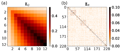
Figure 6: Learned covariance matrices $\bm{\Sigma}_{Q}$ and $\bm{\Sigma}_{N}$ of Graph WaveNet on PEMSD7(M). To make $\bm{\Sigma}_{N}$ more visually identifiable, values greater than 0.1 are mapped to 0.1.

We next try to interpret our results by visualizing the regression coefficient matrices ($\bm{A}$ and $\bm{B}$) and the learned covariance matrices ($\bm{\Sigma}_{N}$ and $\bm{\Sigma}_{Q}$). Figure 4 presents the learned regression coefficient matrices of Graph WaveNet on PEMS08. Figure 4 (a) demonstrates how residuals of spatial locations are correlated to the ones in the past. The residuals of each spatial location are found to be mainly correlated to itself, as suggested by the strong diagonal. While the residuals from some locations are interestingly found important and exhibit strong correlations with other locations. In Figure 4 (b), we also observe a strong diagonal on matrix $\bm{B}$. Since $\bm{B}$ signifies the column effect of the past residual $\bm{R}_{t-\Delta}$ on $\bm{R}_{t}$, the current residual is most correlated to the past residual at the same forecasting step. To visualize the effect of the residual AR process on the model prediction, we plot the base model prediction, final prediction, and residual AR correction in Figure 5. We can observe that the residual AR process serves as a minor correction to the base model prediction (Figure 5 (b)). For the 6-step ahead prediction, the model has difficulty capturing the fast fluctuation of the traffic flow in the further future (Figure 5 (a)). While the residual AR process successfully makes amends for the base model prediction by borrowing information from past residuals.

We also notice that matrices $\bm{A}$ and $\bm{B}$ are almost zero matrices for the traffic speed dataset PEMSD7 (M), suggesting that the temporal autocorrelation is weak the MAE loss collapses the default DL models. In this case, performance improvements on PEMSD7 (M) in Table 2 mainly come from learning the concurrent covariance $\bm{\Sigma}$. Figure 6 presents the learned covariance matrices of Graph WaveNet on PEMSD7 (M). For the covariance matrix $\bm{\Sigma}_{Q}$ that captures the covariance across the forecasting horizon, we can observe that the diagonal of $\bm{\Sigma}_{Q}$ increases with the forecasting step, which is reasonable for multistep forecasting problems. Error propagation in the further forecasting term is also observed, suggested by the increasing covariance between adjacent forecasting steps. Figure 6 (b) captures the covariance of residuals of spatial locations. We can observe certain covariance structures exist for some adjacent locations. The characterizing of such across-step and spatial correlation can regularize the optimization process for better describing the distribution of residuals.

5 Conclusion

In this paper, we present a DR framework to enhance existing seq2seq-based deep traffic forecasting models, which assumes that the residuals are independent with no concurrent spatiotemporal correlation. Our key idea is to properly account for the temporal dependencies in the residual process by modifying the loss function, and this method can be easily integrated into any existing DL model. For simplicity, we model the residual process as a first-order matrix-variate seasonal autoregressive model. This method introduces several additional parameters in DR, including $\bm{A}$, $\bm{B}$, $\bm{\Sigma}_{N}$ and $\bm{\Sigma}_{Q}$, which can be jointly learned with the base deep forecasting model. Through extensive experiments on several state-of-the-art traffic forecasting models using real-world speed and flow datasets, we demonstrate the effectiveness of the proposed methods. We also show that the learned parameters in DR are interpretable with clear physical and statistical meaning, and the learned covariance matrix $\bm{\Sigma}$ can also facilitate probabilistic forecasting with uncertainty quantification. To the best of our knowledge, the proposed method is the first attempt to simultaneously address the spatiotemporal correlation of residuals in multistep (i.e., seq2seq) DL models for traffic forecasting. Despite being primarily designed for traffic forecasting, we believe this method can be adapted for a wide range of seq2seq forecasting problems that exhibit distinct seasonal patterns, such as predicting electricity consumption.

References

- Beach and MacKinnon [1978] Charles M Beach and James G MacKinnon. A maximum likelihood procedure for regression with autocorrelated errors. Econometrica: journal of the Econometric Society, pages 51–58, 1978.
- Breusch [1978] Trevor S Breusch. Testing for autocorrelation in dynamic linear models. Australian economic papers, 17(31):334–355, 1978.
- Chen et al. [2021] Rong Chen, Han Xiao, and Dan Yang. Autoregressive models for matrix-valued time series. Journal of Econometrics, 222(1):539–560, 2021.
- Choi et al. [2022] Seongjin Choi, Nicolas Saunier, Martin Trepanier, and Lijun Sun. Spatiotemporal residual regularization with dynamic mixtures for traffic forecasting. arXiv preprint arXiv:2212.06653, 2022.
- Cochrane and Orcutt [1949] Donald Cochrane and Guy H Orcutt. Application of least squares regression to relationships containing auto-correlated error terms. Journal of the American statistical association, 44(245):32–61, 1949.
- Durbin and Watson [1950] James Durbin and Geoffrey S Watson. Testing for serial correlation in least squares regression: I. Biometrika, 37(3/4):409–428, 1950.
- Godfrey [1978] Leslie G Godfrey. Testing against general autoregressive and moving average error models when the regressors include lagged dependent variables. Econometrica: Journal of the Econometric Society, pages 1293–1301, 1978.
- Guo et al. [2019] Shengnan Guo, Youfang Lin, Ning Feng, Chao Song, and Huaiyu Wan. Attention based spatial-temporal graph convolutional networks for traffic flow forecasting. In Proceedings of the AAAI conference on artificial intelligence, volume 33, pages 922–929, 2019.
- Hsu et al. [2021] Nan-Jung Hsu, Hsin-Cheng Huang, and Ruey S Tsay. Matrix autoregressive spatio-temporal models. Journal of Computational and Graphical Statistics, 30(4):1143–1155, 2021.
- Huang et al. [2020] Qian Huang, Horace He, Abhay Singh, Ser-Nam Lim, and Austin R Benson. Combining label propagation and simple models out-performs graph neural networks. arXiv preprint arXiv:2010.13993, 2020.
- Hyndman and Athanasopoulos [2018] Rob J Hyndman and George Athanasopoulos. Forecasting: principles and practice. OTexts, 2018.
- Jia and Benson [2020] Junteng Jia and Austion R Benson. Residual correlation in graph neural network regression. In Proceedings of the 26th ACM SIGKDD International Conference on Knowledge Discovery & Data Mining, pages 588–598, 2020.
- Kim et al. [2022] Daejin Kim, Youngin Cho, Dongmin Kim, Cheonbok Park, and Jaegul Choo. Residual correction in real-time traffic forecasting. In Proceedings of the 31st ACM International Conference on Information & Knowledge Management, pages 962–971, 2022.
- Li et al. [2018] Yaguang Li, Rose Yu, Cyrus Shahabi, and Yan Liu. Diffusion convolutional recurrent neural network: Data-driven traffic forecasting. In International conference on learning representations, 2018.
- Ljung and Box [1978] Greta M Ljung and George EP Box. On a measure of lack of fit in time series models. Biometrika, 65(2):297–303, 1978.
- Oreshkin et al. [2020] Boris N Oreshkin, Dmitri Carpov, Nicolas Chapados, and Yoshua Bengio. N-beats: Neural basis expansion analysis for interpretable time series forecasting. In International conference on learning representations, 2020.
- Oreshkin et al. [2021] Boris N Oreshkin, Arezou Amini, Lucy Coyle, and Mark J Coates. Fc-gaga: Fully connected gated graph architecture for spatio-temporal traffic forecasting. In Proc. AAAI Conf. Artificial Intell, 2021.
- Prais and Winsten [1954] Sigbert J Prais and Christopher B Winsten. Trend estimators and serial correlation. Technical report, Cowles Commission discussion paper Chicago, 1954.
- Song et al. [2020] Chao Song, Youfang Lin, Shengnan Guo, and Huaiyu Wan. Spatial-temporal synchronous graph convolutional networks: A new framework for spatial-temporal network data forecasting. In Proceedings of the AAAI Conference on Artificial Intelligence, volume 34, pages 914–921, 2020.
- Sun et al. [2021] Fan-Keng Sun, Chris Lang, and Duane Boning. Adjusting for autocorrelated errors in neural networks for time series. Advances in Neural Information Processing Systems, 34:29806–29819, 2021.
- Vlahogianni et al. [2014] Eleni I Vlahogianni, Matthew G Karlaftis, and John C Golias. Short-term traffic forecasting: Where we are and where we’re going. Transportation Research Part C: Emerging Technologies, 43:3–19, 2014.
- Wu et al. [2019] Zonghan Wu, Shirui Pan, Guodong Long, Jing Jiang, and Chengqi Zhang. Graph wavenet for deep spatial-temporal graph modeling. page 1907–1913, 2019.
- Yu et al. [2018] Bing Yu, Haoteng Yin, and Zhanxing Zhu. Spatio-temporal graph convolutional networks: A deep learning framework for traffic forecasting. In Proceedings of the 27th International Joint Conference on Artificial Intelligence, page 3634–3640, 2018.
- Zheng et al. [2020] Chuanpan Zheng, Xiaoliang Fan, Cheng Wang, and Jianzhong Qi. Gman: A graph multi-attention network for traffic prediction. In Proceedings of the AAAI Conference on Artificial Intelligence, volume 34, pages 1234–1241, 2020.