Async-HFL: Efficient and Robust Asynchronous Federated Learning in Hierarchical IoT Networks

Abstract.

Federated Learning (FL) has gained increasing interest in recent years as a distributed on-device learning paradigm. However, multiple challenges remain to be addressed for deploying FL in real-world Internet-of-Things (IoT) networks with hierarchies. Although existing works have proposed various approaches to account data heterogeneity, system heterogeneity, unexpected stragglers and scalability, none of them provides a systematic solution to address all of the challenges in a hierarchical and unreliable IoT network. In this paper, we propose an asynchronous and hierarchical framework (Async-HFL) for performing FL in a common three-tier IoT network architecture. In response to the largely varied networking and system processing delays, Async-HFL employs asynchronous aggregations at both the gateway and cloud levels thus avoids long waiting time. To fully unleash the potential of Async-HFL in converging speed under system heterogeneities and stragglers, we design device selection at the gateway level and device-gateway association at the cloud level. Device selection module chooses diverse and fast edge devices to trigger local training in real-time while device-gateway association module determines the efficient network topology periodically after several cloud epochs, with both modules satisfying bandwidth limitations. We evaluate Async-HFL’s convergence speedup using large-scale simulations based on ns-3 and a network topology from NYCMesh. Our results show that Async-HFL converges 1.08-1.31x faster in wall-clock time and saves up to 21.6% total communication cost compared to state-of-the-art asynchronous FL algorithms (with client selection). We further validate Async-HFL on a physical deployment and observe its robust convergence under unexpected stragglers.

1. Introduction

Embedding intelligence into ubiquitous IoT devices can perform more complex tasks, thus benefiting a wide range of applications including personal healthcare (Beniczky et al., 2021), smart cities (Jasim et al., 2021), and self-driving vehicles (Ahmad and Pothuganti, 2020). To enable distributed learning in a large-scale network, Federated Learning (FL) has appeared as a promising paradigm. The learning procedure begins with the central server distributing the global model to selected devices. Then each device trains with gradient descent on its local dataset and sends the updated model back to the server. Finally, the central server aggregates the received models to obtain a new global model. Edge devices do not reveal the local dataset but only share the updated model. Hence FL collaboratively learns from distributed devices while preserving users’ privacy. The canonical baseline in FL is Federated Averaging (FedAvg) (McMahan et al., 2017) which employs synchronous global aggregation - the central server performs aggregation after the slowest device returns, thus is impeded by unacceptable long delays or stragglers. Recent contributions on semi-asynchronous FL (Chai et al., 2020b; Wu et al., 2020; Zhang et al., 2021; Chen et al., 2022; Nguyen et al., 2022) alleviate the issue by aggregating updates that arrive within a certain period and dealing with late model updates asynchronously. However, the semi-asynchronous scheme still suffers from untimely updates with hard-to-tune waiting periods on heterogeneous and unreliable networks.

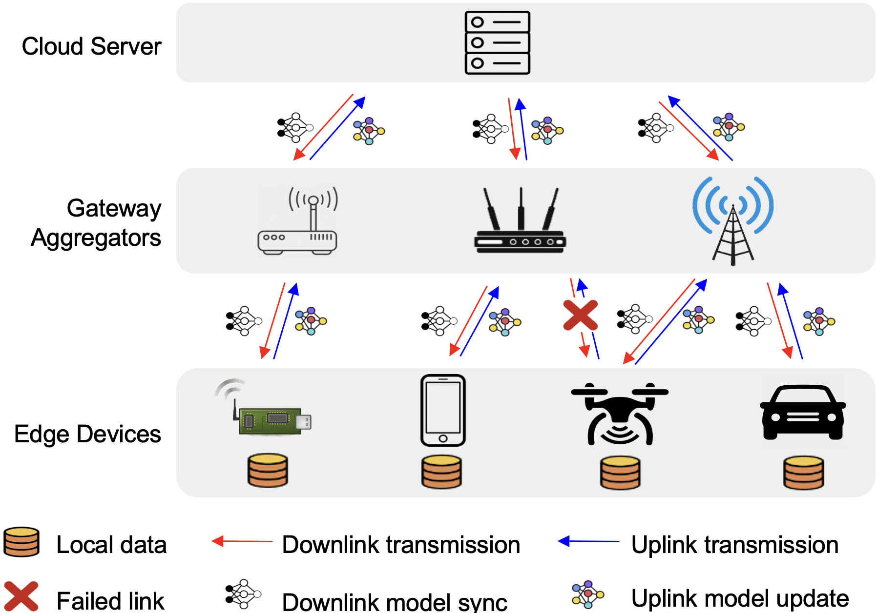
Figure 1. System architecture for a common three-tier IoT networks running FL applications with heterogeneous delays and unreliable networks.

For real-world IoT networks, we recognize that the diverse nature of the overall system prevents an efficient and robust FL deployment. A large number of real deployments are organized in a hierarchical manner, for example, NYCMesh (nyc, 2022), HPWREN (hpw, 2022). All of these architectures can be simplified to the three-tier structure of cloud server, gateway aggregators, and edge devices as shown in Fig. 1. The cloud layer offers powerful servers with abundant resources and effective processing capabilities. The gateway layer includes base stations and routers, acting as an intermediate hub connecting the cloud and edge devices. The bottom layer of edge devices refers to small mobile systems like sensors, smartphones, drones, etc., usually subject to limited resources and energy.

Deploying FL on heterogeneous and hierarchical IoT networks faces the following challenges:

• Heterogeneous data distribution: the distribution of local data on edge devices can be largely different due to environmental variations or users’ specifics. Non-independent and identically distributed (non-iid) data has been shown to slow down or prevent FL convergence without careful and tailored management (Li et al., 2020; Wang et al., 2020b; Karimireddy et al., 2020).

• Heterogeneous system characteristics: The edge devices are equipped with various CPU chips, memory storage and communication technologies. As a result, in Fig. 1, the computational delay on each layer and the communication delay between two layers can be largely different. Applying synchronous and semi-asynchronous FL are subject to longer waiting time.

• Unexpected stragglers (or device dropout): Stragglers are common in every layer of IoT networks, due to energy shortage, circuit shortage or wireless interference. Without careful management, the learning procedure might be delayed or completely hang up due to stragglers.

• Scalability: Naïvely extending a two-tier algorithm to hierarchical networks (3 tiers and more) can lead to significant performance degradation, e.g., unconverged model, significant communication load (Liu et al., 2020). How to preserve the positive gains while avoiding undesired degradation during scaling to hierarchical architectures remains an active research topic.

While previous works have studied how to improve FL convergence under one or two of data heterogeneity (Li et al., 2020; Wang et al., 2020b; Karimireddy et al., 2020), system heterogeneity (Chai et al., 2020a; Lai et al., 2021; Li et al., 2022), unexpected stragglers (Mitra et al., 2021), and hierarchical FL for better scalability (Feng et al., 2022; Zhong et al., 2022), none of existing work provides a systematic solution to address all challenges in a hierarchical and unreliable IoT network. Our work is the first end-to-end framework that uses (i) asynchronous and hierarchical FL algorithm and (ii) system management design to enhance efficiency and robustness, for handling all challenges (C1)-(C4).

In this paper, we propose Async-HFL, an asynchronous and hierarchical framework for performing FL in three-tier and unreliable IoT networks.
$\bullet$ On the algorithmic side, Async-HFL utilizes asynchronous aggregations at both the gateway and the cloud, i.e., the aggregation is performed immediately after receiving a new updated model. Therefore, fast edge devices do not have to wait for the slower peers and stragglers can easily catch up after downloading the latest global model. Compared to naïvely extending existing two-tier asynchronous FL to a three-tier hierarchy, Async-HFL stabilizes convergence and saves communication cost by adding an intermediate gateway aggregation layer.
$\bullet$ Moreover, on the system management side, we propose two modules to improve the performance of asynchronous algorithm under system heterogeneities and stragglers. We design device selection module at the gateway level and device-gateway association module at the cloud level. Gateway-level device selection determines which device to trigger local training in real-time, while cloud-level device-gateway association manages network topology (i.e., which device connects to which gateway) for longer-term performance. Both modules formulate and solve Integer Linear Programs to jointly consider data heterogeneity, system characteristics, and stragglers. For data heterogeneity, we define the learning utility metric to quantify gradient affinity and diversity of devices, inspired from online coreset selection (Yoon et al., 2021). For system heterogeneity, we monitor the latencies per gateway-device link and available connections.
$\bullet$ Async-HFL is different from previous works in that (i) Async-HFL considers finer-grained information of gradient diversity instead of just loss values (as in state-of-the-art asynchronous client selection algorithms (Zhou et al., 2021)), and (ii) Async-HFL incorporates device selection and network topology management at various tiers, which collaboratively optimize model convergence in hierarchical and unreliable IoT networks. To minimize communication overhead, during warm up, we collect the gradients of all devices, perform Principle Component Analysis (PCA) and distribute the PCA parameters to all devices. During training, only the principle components of gradients are exchanged.

In summary, the contributions of Async-HFL are listed as follows:

• Recognizing the unique challenges in hierarchical and unreliable IoT networks, Async-HFL uses asynchronous aggregations at both the gateway and cloud levels. We formally prove the convergence of Async-HFL under non-iid data distribution.

• To quantify data heterogeneity in a finer manner, we propose the learning utility metric based on gradient diversity to guide decision making in Async-HFL.

• To collaboratively optimize model convergence under data heterogeneity, system heterogeneity and stragglers, Async-HFL incorporates distributed modules of the gateway-level device selection and the cloud-level device-gateway association. Communication overhead is reduced by exchanging compressed gradients from PCA.

• We implement and evaluate Async-HFL’s convergence speedup and communication saving under various network characteristics using large-scale simulations based on ns-3 (ns3, 2022) and NYCMesh (nyc, 2022). Our results demonstrate a speedup of 1.08-1.31x in terms of wall-clock convergence time and total communication savings of up to 21.6% compared to state-of-the-art asynchronous FL algorithms. We further validate Async-HFL on a physical deployment with Raspberry Pi 4s and CPU clusters and show robust convergence under stragglers.

Relationship with other FL research: Async-HFL focuses on addressing system variations and potential stragglers in hierarchical IoT networks, thus is orthogonal to other FL techniques of personalization (Tan et al., 2022), pruning (Li et al., 2021a) and masking (Li et al., 2021b). Combining Async-HFL with the above-mentioned techniques is feasible but is not the focus of this paper.

The rest of the paper is organized as follows: Section 2 reviews related works. Section 3 introduces background and models. Section 4 presents a motivating study. Section 5 expands on the details of Async-HFL. Section 6 covers the experimental setups and results. Finally, the whole paper is concluded in Section 7.

2. Related Work

In this section, we review state-of-the-art works and summarize the existing frameworks in Table 1 with regard to challenges (C1)-(C4).

Synchronous FL. Based on FedAvg, a large number of works have studied synchronous FL under data and system heterogeneity from both theoretical and practical perspectives (Li et al., 2020; Wang et al., 2020b; Karimireddy et al., 2020; Chai et al., 2020a; Lai et al., 2021; Mitra et al., 2021). The client (or device) selection procedure can be carefully designed to mitigate heterogeneity by leveraging various theoretical tools (Wang et al., 2020a; Xu et al., 2021a, b; Khan et al., 2020; Ribero and Vikalo, 2020; Balakrishnan et al., 2021). While most works only consider data and computational delay heterogeneity, TiFL (Chai et al., 2020a), Oort (Lai et al., 2021) and PyramidFL (Li et al., 2022) brought up the communication delay variation and implemented smart client selection to balance statistical and system utilities. Nevertheless, all above works consider FL performing in data centers, while long delays and stragglers in unreliable IoT networks can lead to unsatisfied performance with synchrony.

Asynchronous FL. In contrast to synchronous FL, the asynchronous scheme leads to faster convergence under unstable networks especially with millions of devices (Huba et al., 2022). An increasing number of asynchronous FL works have been published in recent years, with focuses on client selection (Hao et al., 2020; Imteaj and Amini, 2020; Zhou et al., 2021; Chen et al., 2021; Zhu et al., 2022), weight aggregation (Wang et al., 2022; You et al., 2022; Wang et al., 2022) and transmission scheduling (Lee and Lee, 2021). Semi-asynchronous mechanisms are developed to aggregate buffered updates (Chai et al., 2020b; Wu et al., 2020; Zhang et al., 2021; Chen et al., 2022; Nguyen et al., 2022). However, how to fully utilize the asynchronous property in hierarchical and heterogeneous IoT systems have not been addressed.

Table 1. Comparing Async-HFL and existing works.

Method	Challenges
	(C1)	(C2)	(C3)	(C4)
Sync FL (two tier)	✓	✓	$\times$	$\times$
Async FL (two tier)	✓	✓	✓	$\times$
Hier. FL ($>$two tier)	✓	✓	$\times$	✓
Async-HFL (three tier)	✓	✓	✓	✓

Hierarchical FL. In hierarchical FL, gateways perform intermediate aggregations before sending their local models to the cloud, so that the backhaul communications between gateways and the cloud are reduced (Liu et al., 2020). Multiple works have formulated client association and resource allocation problems to jointly optimize computation and communication efficiency in synchronous hierarchical FL (Luo et al., 2020; Abad et al., 2020; Liu et al., 2020; Abdellatif et al., 2022). Recent efforts studied mobility-aware (Feng et al., 2022) and dynamic hierarchical aggregations for new data (Zhong et al., 2022). SHARE (Deng et al., 2021) separated the device selection and device-gateway association into two subproblems, then jointly minimized communication cost and shaped data distribution at aggregators for better global accuracy. RFL-HA (Wang et al., 2021) adopts synchronous aggregation within each sub-cluster and asynchronous aggregation between cluster heads (gateways) and the central cloud. All above works employ synchronous aggregation in the system, thus suffering from stragglers.

The only work that studies asynchronous and hierarchical FL is (Wang et al., 2022). In contrast, we provide a systematic framework with additional management modules to adaptively optimize convergence under (C1)-(C4) in real-time.

3. Background

In this section, we provide background on learning model (Section 3.1), system model (Section 3.2) and common techniques in existing two-tier asynchronous FL (Section 3.3). To help the readers get familiar with the notations, we present the list of notations in Table 2. We also depict an example deployment in Fig. 2 which will be referred to as we introduce the models.

Table 2. List of important notations in problem formulation.

Symbol	Meaning	Symbol	Meaning
$\mathcal{C}$	Central cloud	$\mathcal{G}$	Set of $G$ gateways
$\mathcal{N}$	Set of $N$ sensor nodes	$\bm{J}_{t}$	Feasible gateway-sensor links at time $t$
$\bm{I}_{t}$	Connected gateway-sensor links at time $t$	$\tau_{i}^{C}$	Computational delay on device $i$
$\tau_{ji}^{D},\tau_{ij}^{U}$	Downlink and uplink delays between $j$ and $i$	$\tau_{ij}$	Gateway round latency between $j$ and $i$
$R_{ij}$	Average data rate on link $i,j$	$R_{j}$	Data rate of all selected devices at gateway $j$
$B_{j}$	Bandwidth limitation at gateway $j$	$\ell(\bm{\omega};x,y)$	Loss function defined on $\bm{\omega}$ and $(x,y)$
$L^{i}(\bm{\omega})$	Empirical loss function at device $i$	$L_{N}(\bm{\omega})$	Empirical loss function at central cloud
$\mathcal{D}^{i}$	Data distribution at sensor node $i$	$n_{i}$	Number of samples at sensor node $i$
$\bm{\omega}_{h}$	Global model weights after $h$ cloud epochs	$\gamma$	Learning rate at sensor nodes
$\bm{\omega}_{\tau,z}^{j}$	Gateway model at gateway $j$ downloaded from cloud at $\tau$ and aggregated after $z$ gateway epochs	$\bm{\omega}_{\tau,\zeta,e}^{i}$	Sensor model at sensor node $i$ downloaded from gateway at $\zeta$, which the gateway downloaded from the cloud at $\tau$ and aggregated after $e$ device epochs
$H,Z,E$	Number of cloud, gateway and device epochs	$\rho$	Regularization weight in async FL algorithm
$\alpha,\beta$	Exponential decay factor at cloud and gateways	$s(\cdot)$	Staleness function
$u_{i},\eta_{i},v_{i}$	Learning utility, gradients affinity and diversity metric for device $i$	$\kappa,\phi$	Hyperparameter in device selection and association

3.1. Learning Model

Suppose each sensor device $i$ collects data points $(x^{i},y^{i})\sim\mathcal{D}^{i}$ where $\mathcal{D}^{i}$ indicates the underlying data distribution at $i$. We assume all distributions are drawn from the same domain. Non-iid data distribution happens when $\mathcal{D}^{i}\neq\mathcal{D}^{j},\forall i\neq j$. In practice, the underlying distribution $\mathcal{D}^{i}$ is unknown and we only have access to a finite number of $n_{i}$ samples at each device. Note, that $n_{i}$ can be different on various devices and at various time while we omit the time subscript for simplicity. We aim for the typical goal of FL: to learn a uniform model $\bm{\omega}\in\mathbb{R}^{d}$ to be deployed on all distributed devices. Combining with personalized models is also feasible but exceeds the scope of this paper. The loss function $\ell(\bm{\omega};x^{i},y^{i})$ is defined as an error function of how well the model $\bm{\omega}$ performs with respect to sample $(x^{i},y^{i})$. We settle for minimizing the empirical risk minimization problem (ERM) over all devices as follows:

(1) $$\min_{\bm{\omega}\in\mathbb{R}^{d}}L_{N}(\bm{\omega})=\frac{1}{N}\sum_{i=1}^{N}L^{i}(\bm{\omega})=\frac{1}{N}\sum_{i=1}^{N}\frac{1}{n_{i}}\sum_{k=1}^{n_{i}}\ell(\bm{\omega};x_{k}^{i},y_{k}^{i}),$$

Here $L_{N}(\bm{\omega})$ is the global loss function at the central cloud, and $L^{i}(\bm{\omega})$ is the loss function at sensor device $i$.

3.2. System Model

Network topology. In a hierarchical IoT network, suppose $\mathcal{C}$ denotes the central cloud. Let $[n]$ be a set of integers $\left\{1,...,n\right\}$. We define $\mathcal{G}=[G]$ as a set of $G$ gateways (or base stations) and $\mathcal{N}=[N]$ as a large set of $N$ static deployed sensor devices. While all gateways should have feasible paths to the central cloud, there might be multiple gateways that are reachable from one sensor device. Reachability can be limited due to multiple reasons such as range limitation of wireless technology, failed sensor device or network backbones. We combine all above factors into one notation, matrix $\mathbf{J}_{t}\in\mathbb{Z}^{N\times G}$, which indicates the feasible sensor-gateway pairs at wall-clock time $t$:

(2) $$\mathbf{J}_{t,ij}=\left\{\begin{array}[]{ll}1&\textrm{if sensor }i\textrm{ and gateway }j\textrm{ are connectable }\textrm{at time }t\\ 0&\textrm{otherwise}.\end{array}\right.$$

During training, a sensor is associated with only one gateway at one time. The gateway triggers local training on the device, and the device needs to upload the returned model to the same gateway. But sensors can switch to another gateway between aggregations. We use another matrix notation $\mathbf{I}_{t}\in\mathbb{Z}^{N\times G}$ with the same shape as $\mathbf{J}_{t}$ as decision variables for real-time sensor-gateway connections:

(3) $$\mathbf{I}_{t,ij}=\left\{\begin{array}[]{ll}1&\textrm{if sensor }i\textrm{ is connected to gateway }j\textrm{ at time }t\\ 0&\textrm{otherwise}.\end{array}\right.$$

For example, in Fig. 2, sensor device 2 can reach both gateway 1 and 2, but communicates with gateway 1 in the current round. In this case, $\mathbf{J}_{t,21}=\mathbf{J}_{t,22}=1,\mathbf{I}_{t,21}=1,\mathbf{I}_{t,22}=0$.

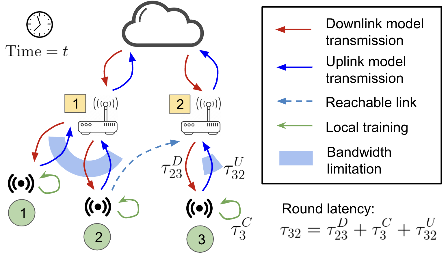
Figure 2. An example of hierarchical FL deployment.

Computational and Communication Models. Computational and communication delays play the major role as system heterogeneities. In this paper, we adopt general models while more specific parameterized CPU or network models (such as (Chen et al., 2020; Luo et al., 2020)) can be applied when more information is given. We are more interested in the communication delays happened on the last-hop links, where bandwidth is more limited and the transmitters (sensor devices) enjoy lower transmission power. During runtime, we measure round latency $\tau_{ij}$ as the time to complete one gateway round between gateway $j$ and sensor $i$, which has three segments: (i) $\tau_{ji}^{D}$, the downlink delay to transmit a model from gateway $j$ to device $i$, (ii) $\tau_{i}^{C}$, the computational delay of device $i$ to perform local training and (iii) $\tau_{ij}^{U}$, the uplink delay to transmit the updated model in a reverse direction. In Fig. 2, the downlink and uplink transmissions are represented with the red and blue arrows, while local training uses green arrow. The round latency is simply the sum of red, green and blue arrows: $\tau_{ij}=\tau_{ji}^{D}+\tau_{i}^{C}+\tau_{ij}^{U}$. The computational delay at gateways and cloud for aggregation are neglected since gateways and cloud generally have more computational resource.

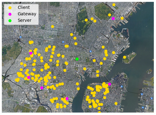
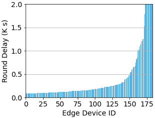
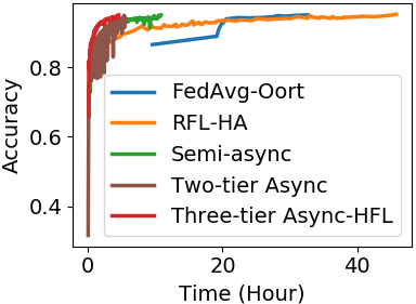
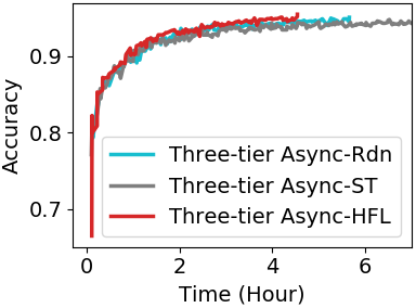
Figure 3. Left: NYCMesh topology. Second left: The round delay distribution of all edge devices. Right: Convergence performance under wall-clock time in the NYCMesh motivating study.

Bandwidth Limitation. Bandwidth limitation places an upper bound on the throughput or data rate. Different from the synchronous design, we cannot accurately model the throughput at $t$ with asynchrony. Therefore, given round latency $\tau_{ij}$ and a FL model with size $M$, we estimate the average data rate on link $i,j$ as $R_{ij}=M/\tau_{ij}$. The total data rate of all selected devices at gateway $j$ can be computed as $R_{j}=\sum_{i=1}^{N}\bm{I}_{ij}R_{ij}$. $B_{j}$ is an upper bound of average data rate on last-hop links at gateway $j$. In Fig. 2, devices 1 and 2 are subject to $B_{1}$, which is depicted as a blue arc.

3.3. Two-Tier Asynchronous FL

In asynchronous FL, each device downloads the latest global model from the cloud, runs local training, and uploads the model to the cloud where asynchronous aggregation is performed immediately. The latest asynchronous FL algorithms (Xie et al., 2019; Chen et al., 2021) employ two common techniques as follows.

Firstly, in addition to the original loss term $L^{i}(\bm{\omega}^{i})$, a regularized loss term penalizing the difference between current model weights $\bm{\omega}^{i}$ and the downloaded global model $\bm{\omega}_{\tau}$ is appended on device $i$:

(4) $$g^{i}(\bm{\omega}^{i};{\bm{\omega}_{\tau}})=L^{i}(\bm{\omega}^{i})+\frac{\rho}{2}\lVert\bm{\omega}^{i}-\bm{\omega}_{\tau}\rVert^{2}.$$

Here $\rho$ is the regularization weight.

Secondly, the algorithm performs staleness-aware weight aggregation at the cloud:

(5a) $$\alpha_{h} \leftarrow\alpha\cdot s(h-\tau)$$

(5b) $$\bm{\omega}_{h} \leftarrow(1-\alpha_{h})\bm{\omega}_{h-1}+\alpha_{h}\bm{\omega}_{new},$$

where $\omega_{new}$ is the newly received model weights, $h$ is the current cloud epoch and $\alpha_{h}$ is the staleness-aware weight calculated by multiplying a constant $\alpha$ with the staleness function $s(h-\tau)$. Staleness refers to the difference in the number of epochs since its last global update. For example, $h$ is the current global aggregating epoch while $\tau$ is the global epoch when the model is downloaded. Intuitively, larger staleness means the model is more outdated and thus should be given less importance. Staleness-aware aggregation simulates an averaging process without synchrony. The staleness function $s(h-\tau)$ determines the exponential decay factor during model aggregation. We adopt the polynomial staleness function $s_{q}(h-\tau)=(h-\tau+1)^{-q}$ parameterized by $q>0$ as in (Xie et al., 2019).

4. A Motivating Study

In this section, we conduct a motivating study of existing FL frameworks under hierarchical and unreliable networks, justifying the design of Async-HFL on both algorithmic and management aspects. While recent works have noticed the importance of accounting the latency factor during client selection (Chai et al., 2020a; Lai et al., 2021; Li et al., 2022), they only considered the delay distribution in a data-center setting which is significantly different from the ones in real-world wireless networks. Real-world measurements have shown that wireless networks follow the long-tail delay distribution and are highly unpredictable (Sui et al., 2016). We implement the FL frameworks based on ns3-fl (Ekaireb et al., 2022) and extract the three-tier topology from the installed node locations in NYCMesh (nyc, 2022) as depicted in Fig. 3 (left). We assume that edge devices are connected to the gateways via Wi-Fi, and the gateways are connected to the server via Ethernet. For each node, we retrieve its latitude, longitude, and height as input to the HybridBuildingsPropagationLossModel in ns-3 to obtain the average point-to-point latency. To include network uncertainties, we add a log-normal delay on top of the mean latency at each local training round. The delay distribution of all edge devices (assuming all devices are selected) in one training round is shown in Fig. 3 (second left). The simulated network delays mimic the measurement results in (Sui et al., 2016). We use the human activity recognition dataset (Anguita et al., 2013), assigning the data collected from one individual to one device thus presenting naturally non-iid data. The upper bound on the bandwidth of the gateways is set to 20KB/s for all experiments.

In such setting, we experiment the performance of (i) FedAvg under Oort, the state-of-the-art latency-aware client selection algorithm (Lai et al., 2021), (ii) RFL-HA (Wang et al., 2021) with asynchronous cloud aggregation and synchronous gateway aggregation, (iii) Semi-async, with synchronous cloud aggregation and semi-asynchronous gateway aggregation as in (Nguyen et al., 2022), (iv) two-tier Async FL which naïvely extends the two-tier asynchronous algorithm (Xie et al., 2019; Chen et al., 2021) to three-tier by letting the gateway just forward data, (v) three-tier Async-HFL with intermediate gateway aggregation proposed in our paper.

Table 3. Total communicated data size ratio (to Async-HFL) before reaching 95% test accuracy in the motivating study.

Sync-Oort	RFL-HA	Semi-async	Two-tier Async
0.79x	1.42x	1.66x	1.30x

We report the wall-clock time convergence in Fig. 3 (right) and the total size of the data communicated in ratio to Async-HFL in Table 3. The convergence of FedAvg and RFL-HA are significantly slowed down even with the state-of-the-art client selection. For Semi-async, we test the waiting period of 50, 100, 150 seconds and select the best results. Semi-async accelerates convergence but still takes 0.39x longer to reach the same 95% accuracy than the fully asynchronous methods. Noticeably, compared to two-tier async, our three-tier Async-HFL achieves more stable and slightly faster convergence, while saving 0.3x communication load (equivalent to 426MB or 1498 multilayer perceptron models). This gain comes from the intermediate gateway aggregation. Introducing an additional “averaging” step does not only smooth out the curve but avoids unnecessary back-and-forth transmission.

Aside from algorithmic design, framework management is also critical in hierarchical FL. We experiment with random (Async-Random), short-latency-first (Async-ST) gateway-level device selection and Async-HFL with full management. The convergence results are shown in Fig. 3 (right). With carefully designed modules, Async-HFL converges 1.24x faster than the random gateway-level device selection. Yet, a poor device selection like Async-ST that ignores data heterogeneity can lead to a 2.13x slower speed to reach 95% accuracy or even an unconverged model in the worst case.

5. Async-HFL Design

5.1. Overview

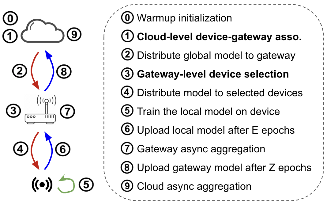
Figure 4. The step-by-step procedure of Async-HFL in one branch of the hierarchical network.

To address all challenges (C1)-(C4) systematically, we propose an end-to-end framework Async-HFL for efficient and robust FL especially in hierarchical and unreliable IoT networks. The major differences between Async-HFL and previous frameworks are the following: (i) Async-HFL quantifies non-iid data distribution by learning utility, which is a metric based on gradient diversity, (ii) Async-HFL incorporates strategic management components, the cloud-level device-gateway association (① in Fig. 4) and the gateway-level device selection (③ in Fig. 4), which are critical in jointly speeding up practical convergence under heterogeneous data and system characteristics.

Fig. 4 depicts the step-by-step procedure of Async-HFL in one round of cloud aggregation. For simplicity, we only show one branch of the hierarchical network. After the warmup initialization, we start from the cloud determining the low-level network topology, namely device-gateway association (①), and then distributing the latest global model to all gateways (②). Next, the gateway distributes the model to devices selected by the gateway (③-④). On the device, local training is performed for $E$ epochs and an updated model is returned to the gateway (⑤-⑥). The gateway then integrates the newly received model immediately using asynchronous aggregation (⑦). After $Z$ gateway updates, the current gateway model is uploaded to the cloud for global asynchronous aggregation (⑧-⑨).

We provide more details on the design of Async-HFL in this section. Section 5.2 presents the detailed asynchronous hierarchical algorithm with convergence proof. Section 5.3 presents the definition of the learning utility metric to quantify gradient diversity. Finally, Section 5.4 reveals the concrete design of device selection and device-gateway association modules.

5.2. Asynchronous Hierarchical FL Algorithm

In Async-HFL, besides the asynchronous cloud aggregation, we utilize an intermediate gateway layer and apply staleness-aware asynchronous aggregation for $Z$ epochs at the gateway. Compared to having the gateways directly forwarding asynchronous model updates to the cloud, adding intermediate gateway aggregations reduces communication burden while making sure the convergence guarantees still apply after adding minimal assumptions (as detailed later). Steps ④-⑦ correspond to the two-tier asynchronous FL in Fig. 4, while our hierarchical algorithm includes steps ②, ④-⑨, spanning all three tiers in the IoT network.

The concrete algorithm implementation on cloud, gateways and devices is shown in Algorithm 1. The cloud and each gateway holds a Cloud or Gateway process, which completes the initialization and asynchronously triggers the Updater threads for aggregation. The Updater thread performs aggregation until the predetermined epoch number is reached. Each sensor device runs a Sensor process that locally solves a regularized optimization problem using stochastic gradient descent (SGD). While previous works have studied adaptively adjusting local epochs according to computational resources (Li et al., 2020), namely trading model quality for faster return, such gain in Async-HFL might be trivial due to asynchronous aggregation and longer as well as unexpected network delays. Hence Async-HFL uses a fixed number of $E$ and $Z$ epochs on device and gateway-level.

Input : $\mathcal{C},\mathcal{G},\mathcal{N},H,Z,E,\alpha,\beta,s(\cdot),g^{i}(\cdot),\bm{\omega}_{0}$

1 Process Cloud()

2       Send $(\bm{\omega}_{0},0)$ to all gateways $j\in\mathcal{G}$

3       Run CloudUpdater() asynchronously in parallel

4Thread CloudUpdater()

5       for cloud epoch $h\in[H]$ do

6             if receive $(\bm{\omega}_{new}^{j},\tau)$ from gateway $j$ then

7                   $\bm{\omega}_{h}\leftarrow(1-\alpha_{h})\bm{\omega}_{h-1}+\alpha\times s(h-\tau)\bm{\omega}_{new}^{j}$

8                   Send $(\bm{\omega}_{h},h)$ to all gateways $j\in\mathcal{G}$

9            

10      

11Process Gateway($j$)

12       if triggered by Cloud() then

13             Receive global model and timestamp $(\bm{\omega}_{h},h)$

14             Update $\tau\leftarrow h,\bm{\omega}_{\tau,0}^{j}\leftarrow\bm{\omega}_{h}$

15             Send $(\bm{\omega}_{\tau,z}^{j},z)$ to selected sensors $i$ connected to $j$

16             Run GatewayUpdater($j$) asynchronously in parallel

17      

18Thread GatewayUpdater($j$)

19       for gateway epoch $z\in[Z]$ do

20             Receive $(\bm{\omega}_{new}^{i},\zeta)$ from sensor node $i$

21             $\bm{\omega}_{\tau,z}^{j}\leftarrow(1-\beta_{z}^{j})\bm{\omega}_{\tau,z-1}^{j}+\beta_{z}^{j}\bm{\omega}_{new}^{i}$

22             Send $(\bm{\omega}_{\tau,z}^{j},z)$ to all sensor $i$ connected to $j$

23      Upload $(\bm{\omega}_{\tau,Z}^{j},\tau)$ to cloud

24Process Sensor($i$)

25       if triggered by Gateway($j$) then

26             Receive $(\bm{\omega}_{\tau,z}^{j},z)$ from gateway $j$

27             Update $\zeta\leftarrow z,\bm{\omega}_{\tau,\zeta,0}^{i}\leftarrow\bm{\omega}_{\tau,z}^{j}$

28             for device epoch $e\in[E]$ do

29                   $\bm{\omega}_{\tau,\zeta,e}^{i}\leftarrow\bm{\omega}_{\tau,\zeta,e-1}^{i}-\gamma\nabla g^{i}(\bm{\omega}_{\tau,\zeta,e-1}^{i};{\bm{\omega}_{\tau,z}^{j}})$

30            Upload $(\bm{\omega}_{\tau,\zeta,E}^{i},\zeta)$ to gateway $j$

31      

Algorithm 1 Asynchronous Hierarchical FL

Convergence Analysis. We now establish the theoretical convergence of Async-HFL’s algorithm. We set the staleness function $s(\cdot)=1$ throughout this section. We require certain regularity conditions on the loss function, namely $L$-smoothness and $\mu$-weak convexity and bounded gradients. Note that $\mu$-weak convexity allows us to handle non-convex loss functions ($\mu>0$), convex functions ($\mu=0$) and strongly convex functions ($\mu<0$). We list the additional assumptions and the convergence result below.

Assumption 1 (Bounded gradients).

The loss function at the cloud, $L_{N}$, and the regularized loss function at each device $g_{i},\,\forall i\in\mathcal{N}$, have bounded gradients bounded by

$$\lVert\nabla L_{N}(\bm{\omega})\rVert^{2}\leq V_{1},\quad\forall\bm{\omega}\in\mathbb{R}^{d}$$

$$\lVert\nabla g^{i}(\bm{\omega};\bm{\omega}^{\prime})\rVert^{2}\leq V_{2},\quad\forall\bm{\omega},\bm{\omega}^{\prime}\in\mathbb{R}^{d},\forall i\in\mathcal{N}.$$

Assumption 2 (Bounded Delay).

The delays $h-\tau$ at the cloud model, and $z-\zeta$ at the gateway model are bounded

(6) $$h-\tau\leq K_{c},\quad\quad\quad z-\zeta\leq K_{g}$$

Assumption 3 (Regularization $\rho$ is large).

$\rho$ is large enough such that for some fixed constant $c>0$, $\forall\tau,\zeta>0,h\geq 1,i\in[N]$,

(7) $$-(1+2\rho+c)V_{1}+\bigg{(}\rho^{2}-\frac{\rho}{2}\bigg{)}\mathbb{E}[\lVert\bm{\omega}_{\tau,\zeta,h-1}^{i}-\bm{\omega}_{\tau,\zeta}^{i}\rVert^{2}]\geq 0$$

Theorem 5.1.

For $L$-smooth and $\mu$-weakly convex loss function $\ell$, under Assumptions 1-3, with $\gamma\leq L^{-1},\alpha\leq K_{c}^{-3/2}$ and $\beta\leq K_{g}^{-3/2}$, after running Algorithm 1 for $H,Z$ and $E$ cloud, gateway and device epochs, we obtain

(8) $$\min_{h=0}^{H-1}\mathbb{E}[\lVert\nabla L_{N}(\bm{\omega}_{h})\rVert^{2}]\leq\frac{\mathbb{E}[L_{N}(\bm{\omega}_{0})-L_{N}(\bm{\omega}_{H})]}{\alpha\beta\gamma cHZE}+\Xi$$

Theorem 5.1 extends the proof of the two-tier asynchronous FL algorithm in (Xie et al., 2019) to three tiers, namely the device-gateway-cloud architecture. Adding the extra gateway level only requires a bounded delay assumption at the gateway and adds constant terms in $\Xi$ due to the gateway, without sacrificing the convergence rate. We are able to ensure convergence in spite of mild assumptions, for instance, constant staleness $s(\cdot)=1$ and weak convexity, and using stronger assumptions would enable even stronger results both theoretically and empirically.

5.3. Learning Utility

To quantify the learning-wise contribution of aggregating each device’s local model to the global model, we need a metric that accounts for data heterogeneity. State-of-the-art asynchronous client selection algorithms (Hu et al., 2021, 2023) use local loss values to indicate the learning contribution of a device. Here in Async-HFL, we propose the learning utility metric which takes into account gradient diversity. Compared to loss values, gradient diversity contains finer-grained information about data heterogeneity.

We extract the latest gradient on device $i$: $\nabla g^{i}(\bm{\mathbf{\omega}}_{\tau,\zeta,E}^{i},\bm{\mathbf{\omega}}_{\tau,z}^{i})$, and global gradient as a sum of all latest gradients: $\nabla L_{N}=\frac{1}{N}\sum_{i=1}^{N}\nabla g^{i}$. The learning utility metric $u_{i}$ is defined for each device $i$ based on the gradient affinity with the global gradient, $\eta_{i}$, and the gradient diversity with the other devices, $\nu_{i}$:

(9a) $$u_{i} =\eta_{i}+\nu_{i},$$

(9b) $$\eta_{i} =\nabla g^{i\top}\nabla L_{N},$$

(9c) $$\nu_{i} =\frac{-1}{N-1}\sum_{j\neq i}^{N-1}\nabla g^{i\top}\nabla g^{j}.$$

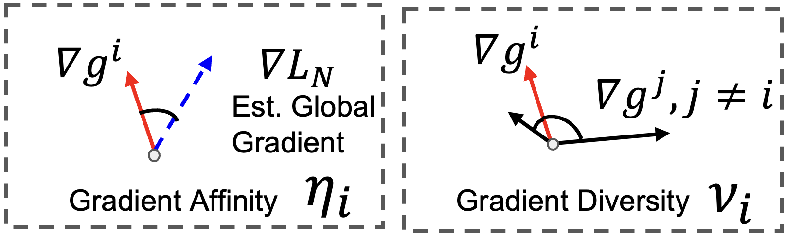
Figure 5. Visualization of the defined learning utility metric combining gradient affinity and gradient diversity.

To assist understanding, a visualization example is shown in Fig. 5. The gradient affinity, $\eta_{i}$, evaluates the similarity between device $i$’s gradients and the global gradients, taking the dot product of $\nabla g^{i}$ and $\nabla L_{N}$ (Equation (9b)). On the other hand, the term $\nu_{i}$ sums up the pairwise dissimilarity between $i$ and all other devices to evaluate the diversity of gradients (Equation (9c)). By combining $\eta_{i}$ and $\nu_{i}$, the learning utility $u_{i}$ is a device-specific metric that favors the devices with close-to-global or largely diverse data distribution. The idea of learning utility is inspired from online coreset selection (Yoon et al., 2021), where the goal is to select a finite number of individual samples that preserve the maximal knowledge about data distribution to store in memory. We stress that our learning utility metric jointly considers the norm and the distribution of gradients, thus integrating more information than just the norm of gradients or loss value.

5.4. Device Selection and Device-Gateway Association

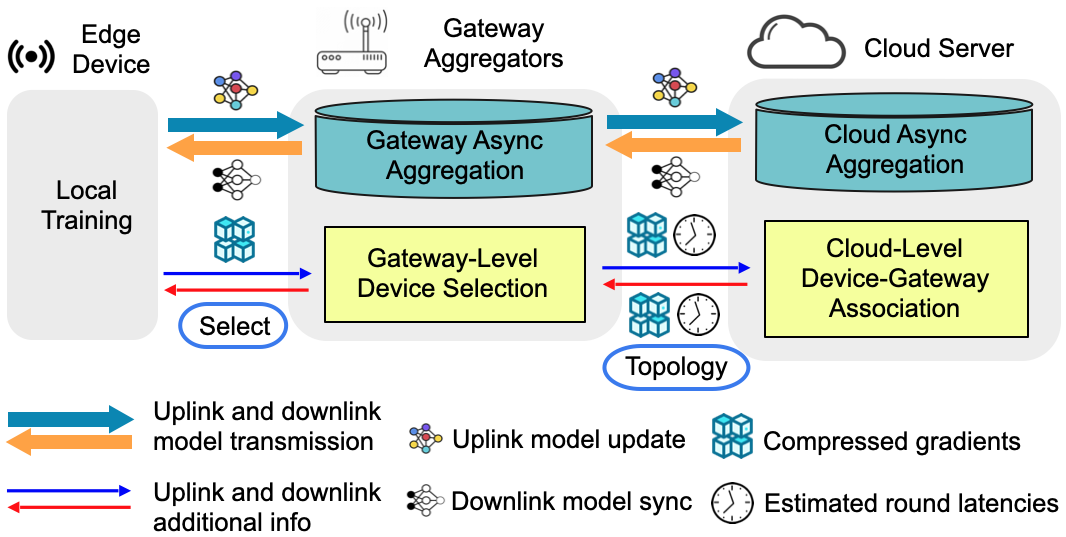
Figure 6. The overview of the distributed design of gateway-level device selection and cloud-level device-gateway association. The thick arrows represent necessary communications for FL while the thin arrows stand for communication overhead.

After identifying the learning utility metric to model data heterogeneity, in this section, we present the design of gateway-level device selection and cloud-level device-gateway association to enhance practical convergence of Async-HFL. Both modules are designed to account diverse data distribution, heterogeneous latencies and unexpected stragglers. Fig. 6 presents an overview of the design and the necessary information to be collected and exchanged. As shown, the gateway-level device selection module executes after the previous gateway aggregation, and thus adjusts device participation in real time. The device-gateway association module is fired less frequently, once after a certain number of cloud epochs, and thus manages network topology for longer-term performance.

Gateway-Level Device Selection. Given the current set of devices connected to gateway $j$ at time $t$ ($\mathbf{I}_{t,ij}=1$), we select a subset to trigger asynchronous training. Suppose $d_{i}=1$ denotes that device $i$ is selected and the latest model is transmitted from the gateway to the device, but the new updated model has not returned from the device. Once returned, the gateway-level device selection module records the compressed gradients information $\nabla g^{i}$ from the device, from which the learning utility $u_{i}$ is updated. We also keep track of the moving average of device’s round latency $\tau_{ij}$ at gateway $j$. In real-time selection, devices presenting large learning utility and short round latency are preferred, as these devices are able to contribute significantly to the convergence in a fast manner. We model the selection problem as an Integer Linear Program with variables of device selecting status $d_{i}$:

(10a) $$\textrm{(Device Selection at}j)\> \max\sum_{\mathbf{I}_{t,ij}=1}d_{i}u_{i}\left(1/\tau_{ij}\right)^{\kappa}$$

(10b) s.t. $$d_{i}R_{ij}\leq B_{j},\quad\forall i\in\left\{i|\mathbf{I}_{t,ij}=1\right\}$$

(10c) $$d_{i}\in\left\{0,1\right\}\quad\forall i\in\left\{i|\mathbf{I}_{t,ij}=1\right\}$$

Equation (10a) defines the objective combining learning utility and round latency, with $\kappa$ as a hyperparameter that curves the contribution of round latency. Equation (10b) imposes the bandwidth upper bound at gateway $j$. The problem has at most $O(|N|)$ variables and linear constraints.

Cloud-Level Device-Gateway Association. Given the feasible links $\mathbf{J}_{t}$ at time $t$, we need to determine the device-gateway association $\mathbf{I}_{t}$ used in the following cloud epochs. We remind the readers that $\mathbf{J}_{t}$ denotes the real-time link availability, so unexpected device or link failures are reflected in $\mathbf{J}_{t}$ and our association solver is able to consider them timely. At the cloud, we retrieve the gradients and round latency information from the corresponding gateways, and send back the decided association $\mathbf{I}_{t}$. Previous works have shown empirically that a stronger similarity of the gateway data distribution to the global distribution leads to a faster method convergence (Deng et al., 2021). To “shape” the gateway distribution while fully utilizing bandwidth, we formulate a multi-objective optimization problem:

(11a) (Association at cloud) $$\max u_{slack}-\phi R_{slack}$$

(11b) s.t. $$\sum_{i=1}^{N}\mathbf{I}_{t,ij}\;u_{i}\geq u_{slack},\quad\forall j\in\mathcal{G}$$

(11c) $$\sum_{i=1}^{N}\mathbf{I}_{t,ij}\;R_{ij}/B_{j}\leq R_{slack},\quad\forall j\in\mathcal{G}$$

(11d) $$\mathbf{I}_{t,ij}\leq\mathbf{J}_{t,ij},\quad\forall i\in\mathcal{N},j\in\mathcal{G}$$

(11e) $$\sum_{j=1}^{G}\mathbf{I}_{t,ij}\leq 1,\quad\forall i\in\mathcal{N}$$

(11f) $$\mathbf{I}_{t,ij}\in\left\{0,1\right\},\quad\forall i\in\mathcal{N}$$

The total objective in Equation (11a) balances the learning utility and the throughput of all associated devices at each gateway. Using slack variables, we are able to disassemble the max-min operation thus keep the problem an Integer Linear Program. The first objective $u_{slack}$ is a slack variable defined as the minimal learning utility among all gateways (Equation (11b)). The second objective $R_{slack}$ is a slack variable for the maximal associated throughput ratio ($R_{j}/B_{j}$) among all gateways (Equation (11c)). Our goal is to make a balanced allocation of devices (considering both learning utility and data rate) which are proportional to the gateways’ bandwidth limitations. $\phi$ is used to tune the importance ratio between sub-objectives. Equation (11d) limits $\mathbf{I}_{t}$ to use feasible links defined by $\mathbf{J}_{t}$. Equation (11e) forces each device to connect to at most one gateway. The problem has $O(|G||N|)$ variables and linear constraints.

The two Integer Linear Programs are in the form of 0-1 Knapsack problem (Fréville, 2004) which can be approached by a large number of algorithms ranging from optimal solver, greedy heuristics to meta-heuristics. In this paper, we implement both problems in the Gurobi solver (Gurobi Optimization, LLC, 2022) and show the computation overhead is negligible in a 200-node network compared to the savings in convergence time.

Minimizing Communication Overhead. The thin arrows in Fig. 6 show the communication overhead, including latest gradients $\nabla g^{i}$, round latencies $\tau_{ij}$ and network topology $\bm{J}_{t},\bm{I}_{t}$. Among these meta information for management, gradients act as the major source of overhead. To minimize the communication overhead of Async-HFL, we first collect all devices’ gradients during warmup, then perform Principle Component Analysis (PCA) on these gradients. Afterwards, we distribute the PCA parameters to all local devices. During the real training session, only the principle components of gradients are exchanged with gateways and clouds. An overhead analysis of Async-HFL is presented in Section 6.7.

6. Evaluation

6.1. Datasets and Models

To simulate heterogeneous data distribution, we retrieve non-iid datasets for four typical categories of IoT applications. The information of the datasets from each category, the partition settings and the models are summarized below.

Table 4. Statistics of federated datasets. Model size refers to the size of the packet that contains all weights in the model.

Dataset	Devices	Avg. Samples/Device	Data Partitions	Models	Size
MNIST	184	600	Synthetic (assign 2 classes to each device)	CNN	1.6MB
FashionMNIST	184	600	Synthetic (assign 2 classes to each device)	CNN	1.7MB
CIFAR-10	50	1000	Synthetic (assign 2 classes to each device)	ResNet-18	43MB
Shakespeare	143	2892.5	Natural (each device is a speaking role)	LSTM	208KB
HAR	30	308.5	Natural (each device is a human subject)	MLP	285KB
HPWREN	26	6377.4	Natural (each device is a station)	LSTM	292KB

Application #1: Image Classification. We select MNIST (Deng, 2012), FashionMNIST (Xiao et al., 2017), CIFAR-10 (Krizhevsky et al., 2009) datasets for evaluation. We apply CNNs with two convolutional layers for MNIST and FashionMNIST, and the canonical ResNet-18 (He et al., 2016) for CIFAR-10. All three image classification datasets are partitioned synthetically with 2 classes randomly assigned to each device, and the local samples are dynamically updated from the same distribution.

Application #2: Next-Character Prediction. We adopt the Shakespeare (Caldas et al., 2018) dataset, where the goal is to correctly predict the next character given a sequence of 80 characters. Local data is partitioned by assigning the dialogue of one role to one device. We apply a two-layer LSTM classifier containing 100 hidden units with an 8D embedding layer, which is the base model for this application.

Application #3: Human Activity Recognition. We use the HAR dataset (Anguita et al., 2013) collected from 30 volunteers. We assign the data from one individual to one device and apply a typical multilayer perceptron (MLP) model with two fully-connected layers.

Application #4: Time-Series Prediction. We build a time-series prediction task using the historical data collected by the High Performance Wireless & Education Network (HPWREN) (hpw, 2022). HPWREN is a large-scale environmental monitoring sensor network spanning 20k sq. miles and collecting readings of temperature, humidity, wind speed, etc., every half an hour. Each reading has 11 features and we combine the readings in the past 24 hours (in total 48 readings) to be one sample. Each device holds the data collected at one station. The goal is to predict the next reading. We use the mean squared error (MSE) loss and a one-layer LSTM with 128 hidden units.

6.2. System Implementation

As each trial of FL on a large physical deployment can take up to days, we mainly use simulations to mimic practical system and network heterogeneities. We further implement and validate Async-HFL on a smaller physical deployment.

Large-Scale Simulation Setup. We implement our discrete event-based simulator based on ns3-fl (Ekaireb et al., 2022), the state-of-the-art FL simulator using PyTorch for FL experiments and ns-3 (ns3, 2022) for network simulations. Note, that in contrast to most existing frameworks that simulate communication rounds (Li et al., 2019; Xie et al., 2019; Wang et al., 2020b; Karimireddy et al., 2020), ns3-fl simulates the wall-clock computation and communication time based on models from realistic measurements. Approaches showing superb convergence with regard to rounds might perform poorly under wall-clock time if failing to consider system heterogeneities. The network topology is configured based on NYCMesh as described in Section 4 with 184 edge devices, 6 gateways, and 1 server.

Physical Deployment Setup. We implement Async-HFL on Raspberry Pi (RPi) 4B and 400 based on the state-of-the-art framework FedML (Chaoyang He, 2020). The physical deployment consists of 7 RPi 4Bs and 3 RPi 400s, distributing in 7 different houses and all connecting to the home Wi-Fi router. We ensure the variances of networking conditions by setting up some RPis in the farther end of the backyard, some in the bedroom in the vicinity of the router. We stress that the networking conditions may also be affected by the Wi-Fi traffic in real time. For example, the network delay could be longer if the residents are streaming a movie in the meantime. Such setup mimics the real-world scenarios where our application shares the bandwidth with other traffic and the network latency enjoys high diversity. In addition, during our experiment, we observe that RPis may fail to connect from the beginning, or (with rare probabilities) encounter unexpected suspension in the middle of one trial. Creating two virtual clients on each RPi, we are able to obtain a total of 20 clients on the RPi setup.

Apart from the RPis, we set up 20 more clients by requesting 1, 2 or 4 CPU cores from a CPU cluster and each accompanied by 4 GB RAM. Different from the RPi clients, where networking conditions vary largely, the CPU cluster has a stable internet connection but the computational delay varies depending on the requested resource. Since we do not have access to the home Wi-Fi router, we deploy the implementation of gateways and the cloud on an Ethernet-connected desktop, with an Intel Core i7-8700@3.2GHz, 16GB RAM and a NVIDIA GeForce GTX 1060 6GB GPU.

6.3. Experimental Setup

Table 5. Important parameters setup on various datasets.

Dataset	Target Acc./Err.	Gateway	$\gamma$	$\rho$
MNIST	95	1M	0.01	0.1
FashionMNIST	75	1M	0.01	0.1
CIFAR-10	50	20M	0.001	1.0
Shakespeare	35	20k	0.01	0.2
HAR	95	20K	0.003	0.1
HPWREN	1.5e-5 (pred. err.)	20K	0.001	0.1

Table 6. Convergence speedup on large-scale simulations and various datasets. Bolded numbers reflect the best baseline result on each dataset.

Dataset	Convergence time speedup of Async-HFL with respect to baselines
	Async-HL	Async-Random	Semi-async	RFL-HA	Sync-Oort	Sync-TiFL	Sync-DivFL	Sync-Random
MNIST	1.11x	1.27x	6.2x	32.5x	40.0x	27.13x	63.4x	67.3x
FashionMNIST	1.08x	1.49x	8.3x	36.7x	20.5x	32.8x	73.4x	96.8x
CIFAR-10	1.09x	1.40x	2.3x	12.3x	44.3x	59.0x	62.0x	61.7x
Shakespeare	1.19x	1.79x	0.59x	0.71x	0.31x	2.39x	5.87x	5.46x
HAR	1.31x	1.22x	2.7x	7.4x	10.3x	21.6x	22.5x	24.1x
HPWREN	1.11x	1.48x	2.4x	12.8x	19.5x	26.5x	27.7x	31.4x

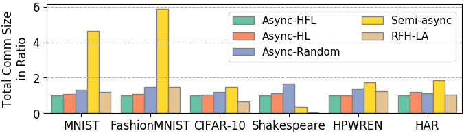
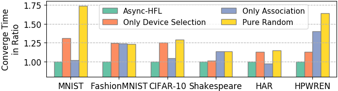
Figure 7. Left: Total communicated data size in ratio compared to Async-HFL on large-scale simulations and various datasets. Right: Convergence time in ratio compared to Async-HFL using various combinations of device selection and device-gateway association.

Baselines. Given that the major design of Async-HFL is around device selection and association, we adopt state-of-the-art client-selection methods from the synchronous, hybrid, semi-asynchronous, and asynchronous FL schemes to compare. We add the prefix sync to the baselines using synchronous aggregations at both gateway and cloud. Conversely, async indicates asynchronous aggregations at both gateway and cloud. The only two baselines not following this naming rule are RFL-HA and Semi-async as follows.

• Sync-Random/TiFL/Oort/DivFL makes random device-gateway association while device selections are made via random selection, TiFL (Chai et al., 2020a), Oort (Lai et al., 2021) and DivFL (Balakrishnan et al., 2021) respectively. TiFL groups devices with similar delays to one tier and greedily selects high-loss devices in one tier until reaching the throughput limit. Oort uses a multi-arm bandits based algorithm to balance loss and latency. DivFL utilizes a greedy method to maximize a submodular function which takes the diversity of gradients into account.

• RFL-HA (Wang et al., 2021) uses synchronous aggregation at gateways and asynchronous aggregation at cloud. While applying a random device selection at the gateway level, RFL-HA utillizes a re-clustering heuristic to adjust device-gateway associations.

• Semi-async performs semi-asynchronous aggregations at gateways as in (Nguyen et al., 2022) and synchronous aggregations at cloud. Random choices are applied for device selection and device-gateway association. We experiment with the semi-period of 50, 100, 150 seconds and pick the best results.

• Async-Random/HL uses random device-gateway association and random or high-loss first device selection under the asynchronous scheme. Prioritizing the nodes with high loss or large gradients’ norm is the state-of-the-art approach for asynchronous FL (Hu et al., 2021, 2023). We did not compare with (Zhu et al., 2022) as their algorithm depends on completely different metrics.

Evaluation Metrics. For the simulation, we compare the convergence time, i.e., the wall-clock time to reach a predetermined accuracy or test loss (i.e., loss on the test dataset). Detailed parameters setup are listed in Table 5. The target accuracy or loss is close to the optimal value that is reached by FedAvg. We also compare the total communicated data size to account communication efficiency. For the physical deployment, we quantify convergence using the accuracy or test loss at the same wall-clock elapsed time. We also study the execution time, which is indicative of energy consumption on real platforms.

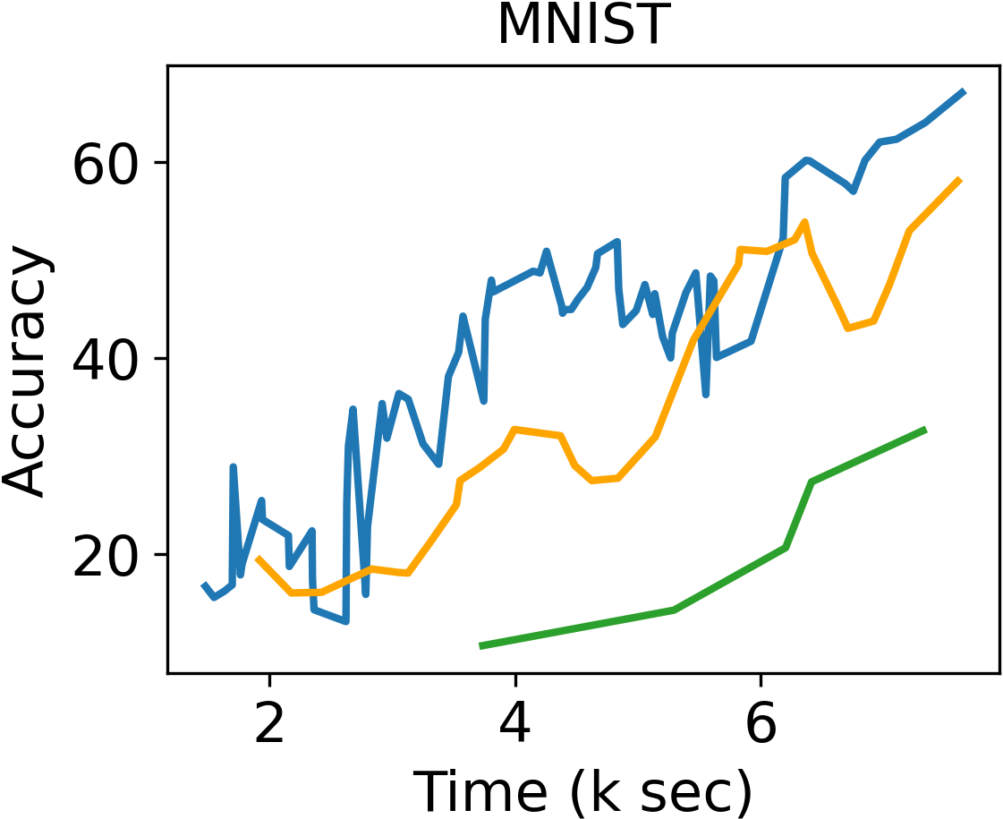
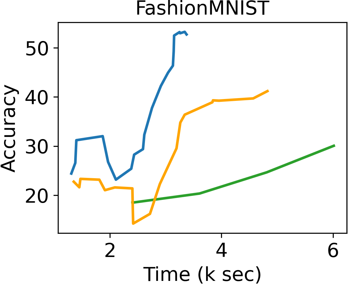
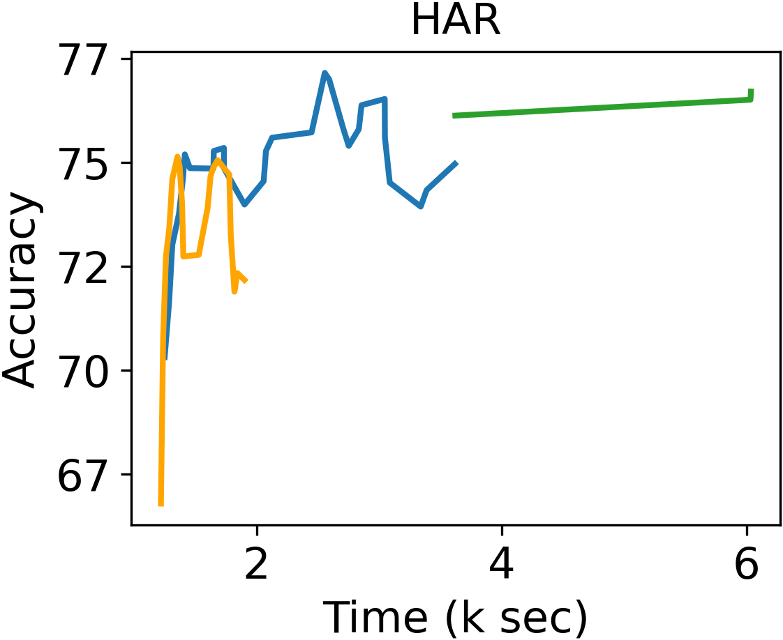
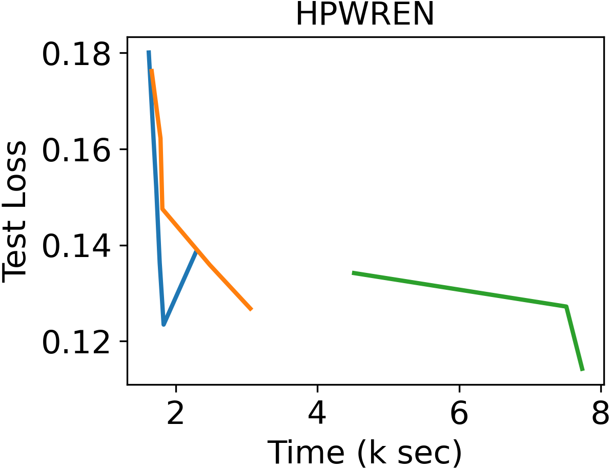
Figure 8. Convergence results under wall-clock time on the physical deployment.

6.4. Results on Large-Scale Simulations

Convergence Results. We first report the simulated convergence time on all datasets using NYCMesh topology. We set device epochs $E=5$ and gateway epochs $Z=20$ for asynchronous, $Z=5$ for semi-asynchronous and synchronous gateway aggregations. Each method is tested with three random trials and we report the average convergence time and the corresponding speedup in Table 6. On all three image classification datasets, Async-HFL achieves a minimum 1.11x, 1.08x, 1.09x speedup over the best baseline. On HAR and HPWREN datasets (with smaller number of devices, see Table 4) Async-HFL surpasses the best baseline by 0.22x and 0.11x respectively. Hence the design of Async-HFL to balance learning utility and system characteristics works under both synthetic and nature data partition. The only exception is Shakespeare, where Sync-Oort, RFL-HA and semi-async reach the target accuracy faster than Async-HFL. Nevertheless, we emphasize that Async-HFL still has 1.19x speedup compared to the state-of-the-art asynchronous FL. We speculate that the relative slower convergence of all asynchronous methods on Shakespeare roots in the essential converging difficulty of two-tier asynchronous FL algorithms. In the convergence curve of Shakespeare, we observe the first test accuracy increase with asynchronous methods after around 100 cloud epochs, while the synchronous baseline improves test accuracy at the first cloud epoch. We will refine the algorithmic design of Async-HFL for efficient convergence on Shakespeare in our future work. In general, synchronous methods take much longer to reach the target accuracy due to the long waiting time, even with delay-aware client selection methods such as Oort and TiFL. Both RFL-HA and Semi-async leverage hybrid aggregation scheme, thus converge slower than the fully asynchronous methods while faster than the synchronous approaches, except on Shakespeare. The convergence speedup of Async-HFL over state-of-the-art asynchronous methods is 1.08-1.31x on all datasets.

The total communicated data size of non-synchronous methods compared to Async-HFL is shown in Fig. 7 (left). We are only interested in comparing non-synchronous methods as synchronous aggregation trades long waiting time for less cloud epochs and communication savings. Therefore, synchronous methods take much less communication to converge but the slowdown is usually unacceptable as shown in Table 6. Async-HFL saves total communicated data size by 2.6%-21.6% and 14.5%-66.8% compared to Async-HL and Async-Random on all datasets. The total transmitted data size of semi-async and RFL-HA on Shakespeare is significantly lower than asynchronous approaches due to their fast convergence. Note, that on CIFAR-10, although RFL-HA consumes only 0.65x exchanged data compared to Async-HFL, it takes 11.3x longer to reach the same accuracy. The hybrid schemes of RFL-HA and Semi-async do not end up with faster convergence nor communication savings on MNIST, FashionMNIST, HPWREN and HAR.

Performance Breakdown. Async-HFL includes two modules to boost the FL performance: gateway-level device selection and cloud-level device-gateway association. To evaluate the contribution of each component separately, we compare the convergence time on all datasets using (i) pure random selections, (ii) only the device selection, (iii) only the device-gateway association, and (iv) the complete Async-HFL as shown in Fig. 7 (right). The target accuracy and bandwidth are set to the same as in Table 5. Each module contributes various extents on different datasets. On MNIST, CIFAR-10 and HAR, the device-gateway association improves convergence more significantly by balancing the network topology, achieving 1.71x, 1.23x and 1.17x speedup by itself. On FashionMNIST, using one module does not change much, but applying both modules leads to a 1.23x speedup. On Shakespeare, the speedup is mainly supported by our coreset device selection with a 1.12x speedup by itself. On HPWREN, applying a single device selection or device-gateway association module leads to a 1.45x or 1.17x speedup, while using both modules contributes to a 1.64x total speedup. Hence both device selection and association components are necessary in Async-HFL to deal with various data and system heterogeneities.

6.5. Results on Physical Deployment

Convergence Results. We validate Async-HFL on the physical deployment running MNIST, FashionMNIST, HAR and HPWREN datasets. The accuracy or test loss under wall-clock time are summarized in Fig. 8. We run Async-HFL and Async-HL for 30 cloud rounds, Sync-Random for 3 cloud rounds, unless the system is suspended due to stragglers. Note, that Async-HL is the state-of-the-art asynchronous baseline and presents the second best result in simulations. Async-HFL ends up with 70%, 56% and 75% accuracies on MNIST, FashionMNIST and HAR, while Async-HL only reaches 62%, 36% and 73% at similar time (after 7.6K, 3.4K and 2K seconds). For the synchronous baseline, we are only able to obtain very limited traces due to straggler effects. After setting a timeout limit for synchronous aggregations, we acquire the curves in Fig. 8 with very slow convergence. The HPWREN dataset is very computational challenging for all methods and a lot of devices drop off due to no communication for a long time. Async-HFL strives for convergence within 2K seconds, while Async-HL and Sync-Random reach similar test loss after 3K and 7.7K seconds. While a small-scale physical deployment can be largely affected by uncertainties, we are able to observe consistently better convergence using Async-HFL over the baselines on all four datasets. The results demonstrate the robustness of Async-HFL under delay heterogeneities and stragglers. This is because the Async-HFL performance is dynamically guided by its two modules: (i) the gateway-level device selection module, which timely adjusts device participation, and (ii) the cloud-level device-gateway association, which considers device dropouts via taking $\mathbf{J}_{t}$ as input.

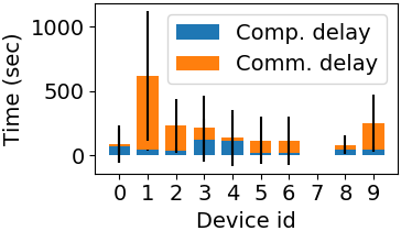
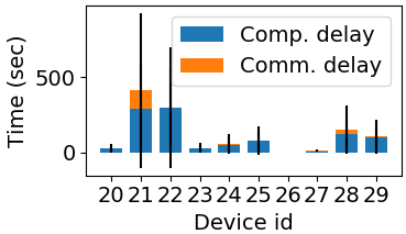
Figure 9. Round latency results on the physical deployment running MNIST. Left: Time breakups on RPis. Right: Time breakups on CPUs.

Round Latency. Fig. 9 displays the round latency measurements of our practical setup, which demonstrates how challenging our physical deployment is. To remind the reader, round latency is the time to complete one gateway round of downloading the model to device, training the model on device, then returning the updated model back to the gateway. The measurement supports our argument that IoT networks present heterogeneous system and network characteristics. In more details, Fig. 9 left and right show the round latency breakup on ten representatives of RPis and CPU clusters respectively. The missing columns indicate failed devices. Our physical deployment setup covers two typical scenarios with very different breakups. For RPis, the major heterogeneity comes from the network side, as we setup the RPis at various places with different distances to the router. For CPU clusters, the computational delay rather than communication delay presents more variations due to varying number of requested CPU cores. For FL, both heterogeneities cause the largely varied and unstable round latency distribution that Async-HFL targets to address.

6.6. Sensitivity Analysis.

Bandwidth Limitation. Fig. 10 (left) shows the convergence time to reach 95% on MNIST when altering bandwidth limits at all gateways. The speedup over Async-Random is more significant under more restricted bandwidth (3.47x under 0.5MB/s vs. 0.56x under 2MB/s), as the benefit of intelligently selecting subset of devices reveals more with limited resource. Compared to the Sync-Random baseline, the speedup gap closes under 0.5MB/s bandwidth. When only a limited number of devices can be selected, FedAvg (Sync-Random) gets a stable convergence via averaging the models from multiple devices.

Target Accuracy. Fig. 10 (right) shows the convergence time to reach various target accuracies on MNIST with the same set of other settings. The speedup over Async-Random is 1.99x, 1.50x and 1.34x for reaching 85%, 90% and 95%. Under the same settings, the speedup over Sync-Random is 106x, 78x and 51x. The results demonstrate Async-HFL’s fast convergence in the early stage, which can be attributed to prioritizing diverse and fast devices in Async-HFL’s management design.

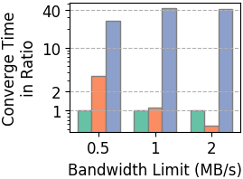
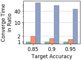
Figure 10. Convergence time in ratio compared to Async-HFL running MNIST under various bandwidth limits at gateways (left) and target accuracy (right) at cloud.

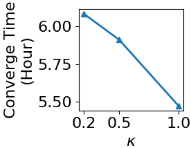
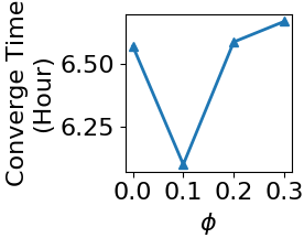
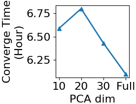
Figure 11. Sensitivity experiments of Async-HFL on HAR dataset.

Hyperparameters $\kappa$ and $\phi$. We experiment the impact of $\kappa$ (Equation (10a)) and $\phi$ (Equation (11a)) on the final convergence time, as both parameters determine the balance between data heterogeneity (learning utility) and system heterogeneity (round latency). We use the HAR dataset with configurations in Table 5. Fig. 11 (left) shows the wall-clock time to reach the same accuracy using $\kappa=0.2,0.5,1.0$. A larger $\kappa$ increases the weight of delays during gateway-level device selection thus results in faster convergence. Fig. 11 (middle) depicts the wall-clock convergence time using $\phi=0,0.1,0.2,0.3$. $\phi=0$ means only data heterogeneity is considered, while a larger $\phi$ increases the contribution of bandwidth limitation during cloud-level device-gateway association. A proper $\phi$ (in this case, $\phi=0.1$) leads to the best convergence performance by jointly considering data and system aspects.

6.7. Overhead Analysis

As shown in Fig. 6, the major communication overhead of Async-HFL comes from exchanging the gradients. Using PCA to compress the gradients, the effect of various PCA dimensions on convergence time while processing the HAR dataset is shown in Fig. 11 (right). A PCA compression of 30 dimensions introduces a communication overhead of ¡0.5%, while the increase on convergence time (compared to using the full gradients) is less than 6%. Hence, the PCA compression strategy effectively reduces communication overhead while preserving convergence speed. On the computational side, the device selection algorithm consumes 1.6, 1.4, 4.3, 0.1 seconds per selection on the MNIST, FashionMNIST, CIFAR-10 and Shakespeare datasets. The time consumption of cloud-level association is 1.1, 0.9, 8.7 and 0.3 seconds per selection on the server for the above datasets. These additional computational times are negligible on the physical deployment with an average 120.26 seconds of round latency.

7. Conclusion

In this paper, we propose Async-HFL, the first end-to-end asynchronous hierarchical Federated Learning framework which jointly considers data, system heterogeneities, stragglers and scalability in IoT networks. Async-HFL performs asynchronous aggregations on both gateways and cloud, thus achieving faster convergence with heterogeneous delays and being robust to stragglers. With the learning utility metric to quantify gradient diversity, we design the device selection and device-gateway association modules to balance learning utility, round latencies and unexpected stragglers, collaboratively optimizing practical model convergence. We conduct comprehensive simulations based on ns-3 and NYCMesh to evaluate the Async-HFL under various network characteristics. Our results show a 1.08-1.31x speedup in terms of wall-clock convergence time and 2.6-21.6% communication savings compared to state-of-the-art asynchronous FL algorithms. Our physical deployment proves robust convergence under unexpected stragglers.

Appendix A Proof of Theorem 5.1

In the main paper, we establish the convergence of Async-HFL under the three assumptions. Our analysis extends the proof in (Xie et al., 2019) from a single level of asynchrony to two levels. The proof involves bounding the deviation of cloud loss function $L_{N}$ between steps in terms of its gradient norm $\nabla L_{N}$. We proceed from the lowest level, the device, establishing progress across device steps $e$. Then, using the progress after $E$ device steps, we can then bound progress at the next level, which is the gateway. Note that moving to the next level, the cloud is much simpler as the update steps and assumptions for cloud and gateway level are similar. We now describe the complete proof starting from the progress on any device in the next subsection.

A.1. Device steps

On each device, we only perform SGD steps, therefore, we can utilize Assumptions 1 and  3 to bound the progress after each gradient update.

Lemma A.1 (Single-step Device).

Under Assumptions 1 and  3, the progress in terms of $L_{N}$ after one device step is given by

(12) $$\mathbb{E}[L_{N}(\bm{\omega}_{\tau,\zeta,e}^{i})]\leq \mathbb{E}[L_{N}(\bm{\omega}_{\tau,\zeta,e-1}^{i})]-\gamma c\mathbb{E}[\lVert\nabla L_{N}(\bm{\omega}_{\tau,\zeta,e-1}^{i})\rVert^{2}]$$

$$+\gamma^{2}\mathcal{O}(\rho E^{2}V_{2})\quad\forall\tau,\zeta\geq 0,e\geq 1,i\in\mathcal{N}$$

Proof.

Since the loss is $L$-smooth, $L_{N}(\bm{\omega})$ and $g_{N,\bm{\omega}^{\prime}}(\bm{\omega})$ are $L$-smooth and $(2L+2\rho)$-smooth. To simplify the proof, we drop the subscript $\tau$ and superscript $i$ from the following steps. Since $g_{N,\bm{\omega^{\prime}}}(\bm{\omega})\geq L_{N}(\bm{\omega})\forall\bm{\omega},\bm{\omega^{\prime}}$, we have

$$\mathbb{E}[L_{N}(\bm{\omega}_{\zeta,e})] \leq\mathbb{E}[g_{N,\bm{\omega}_{\zeta}}(\bm{\omega}_{\zeta,e})]$$

$$\leq\mathbb{E}[g_{N,\bm{\omega}_{\zeta}}(\bm{\omega}_{\zeta,e-1})]+\gamma^{2}(L+\rho)\mathbb{E}[\lVert\nabla g_{\bm{\omega}_{\zeta}}(\bm{\omega}_{\zeta,e-1})\rVert^{2}]$$

$$\quad-\gamma\mathbb{E}[\left\langle\nabla g_{N,\bm{\omega}_{\zeta}}(\bm{\omega}_{\zeta,e-1}),\nabla g_{\bm{\omega}_{\zeta}}(\bm{\omega}_{\zeta,e-1})\right\rangle]$$

$$\leq\mathbb{E}[L_{N}(\bm{\omega}_{\zeta,e-1})]+\frac{\rho}{2}\mathbb{E}[\lVert\bm{\omega}_{\zeta}-\bm{\omega}_{\zeta,e-1}\rVert^{2}]$$

$$\quad+\gamma^{2}(L+\rho)\mathbb{E}[\lVert\nabla g_{\bm{\omega}_{\zeta}}(\bm{\omega}_{\zeta,e-1})\rVert^{2}]$$

$$\quad-\gamma\mathbb{E}[\left\langle\nabla g_{N,\bm{\omega}_{\zeta}}(\bm{\omega}_{\zeta,e-1}),\nabla g_{\bm{\omega}_{\zeta}}(\bm{\omega}_{\zeta,e-1})\right\rangle]$$

$$\leq\mathbb{E}[L_{N}(\bm{\omega}_{\zeta,e-1})]+\frac{\rho\gamma^{2}E^{2}V_{2}}{2}+\gamma^{2}(L+\rho)V_{2}$$

$$\quad-\gamma\mathbb{E}[\left\langle\nabla g_{N,\bm{\omega}_{\zeta}}(\bm{\omega}_{\zeta,e-1}),\nabla g_{\bm{\omega}_{\zeta}}(\bm{\omega}_{\zeta,e-1})\right\rangle]$$

For the second step, we use smoothness of $g_{N,\bm{\omega}_{\zeta}}$. For the third step, we expand $g_{N,\bm{\omega}_{\zeta}}$ and for the fourth step, we use Assumption 1 to bound $\mathbb{E}[\lVert\nabla g_{\bm{\omega}_{\zeta}}(\bm{\omega}_{\zeta,e-1})\rVert^{2}]$ and $\mathbb{E}[\lVert\bm{\omega}_{\zeta}-\bm{\omega}_{\zeta,e-1}\rVert^{2}]$.

Note that, $\mathbb{E}[\lVert\bm{\omega}_{\zeta}-\bm{\omega}_{\zeta,e-1}\rVert^{2}]=\mathbb{E}[\lVert\sum_{r=1}^{e-1}\gamma\nabla g_{\bm{\omega}_{\zeta}}(\bm{\omega}_{\zeta,r})\rVert^{2}]\leq\gamma^{2}(e-1)\sum_{r=1}^{e-1}\mathbb{E}[\lVert\nabla g_{\bm{\omega}_{\zeta}}(\bm{\omega}_{\zeta,r})\rVert^{2}]\leq\gamma^{2}(e-1)^{2}V_{2}\leq\gamma^{2}E^{2}V_{2}$

We now utilize Assumption 3 to bound the remaining terms and introduce $\nabla L_{N}$. Consider the following inequality for some $c>0$,

$$\mathbb{E}[\left\langle\nabla g_{N,\bm{\omega}_{\zeta}}(\bm{\omega}_{\zeta,e-1}),\nabla g_{\bm{\omega}_{\zeta}}(\bm{\omega}_{\zeta,e-1})\right\rangle]-c\mathbb{E}[\lVert\nabla L_{N}(\bm{\omega}_{\zeta,e-1})\rVert^{2}]$$

$$=\mathbb{E}[\langle\nabla L_{N}(\bm{\omega}_{\zeta,e-1})+\rho(\bm{\omega}_{\zeta,e-1}-\bm{\omega}_{\zeta}),$$

$$\quad\nabla L(\bm{\omega}_{\zeta,e-1})+\rho(\bm{\omega}_{\zeta,e-1}-\bm{\omega}_{\zeta})\rangle]-c\mathbb{E}[\lVert\nabla L_{N}(\bm{\omega}_{\zeta,e-1})\rVert^{2}]$$

$$=\mathbb{E}[\left\langle\nabla L_{N}(\bm{\omega}_{\zeta,e-1}),\nabla L(\bm{\omega}_{\zeta,e-1})\right\rangle]+\rho^{2}\mathbb{E}[\lVert\bm{\omega}_{\zeta,e-1}-\bm{\omega}_{\zeta}\rVert^{2}]$$

$$\quad+\rho\mathbb{E}[\left\langle\nabla L_{N}(\bm{\omega}_{\zeta,e-1})+\nabla L(\bm{\omega}_{\zeta,e-1}),\bm{\omega}_{\zeta,e-1}-\bm{\omega}_{\zeta}\right\rangle]$$

$$\quad-c\mathbb{E}[\lVert\nabla L_{N}(\bm{\omega}_{\zeta,e-1})\rVert^{2}]$$

$$\geq-\frac{1}{2}\mathbb{E}[\lVert\nabla L_{N}(\bm{\omega}_{\zeta,e-1})\rVert^{2}]-\frac{1}{2}\mathbb{E}[\lVert\nabla L(\bm{\omega}_{\zeta,e-1})\rVert^{2}]$$

$$\quad+\rho^{2}\mathbb{E}[\lVert\bm{\omega}_{\zeta,e-1}-\bm{\omega}_{\zeta}\rVert^{2}]-\frac{\rho}{2}\mathbb{E}[\lVert\bm{\omega}_{\zeta,e-1}-\bm{\omega}_{\zeta}\rVert^{2}]$$

$$\quad-\frac{\rho}{2}\mathbb{E}[\lVert\nabla L_{N}(\bm{\omega}_{\zeta,e-1})+\nabla L(\bm{\omega}_{\zeta,e-1})\rVert^{2}]-c\mathbb{E}[\lVert\nabla L_{N}(\bm{\omega}_{\zeta,e-1})\rVert^{2}]$$

$$\geq-\frac{1}{2}\mathbb{E}[\lVert\nabla L_{N}(\bm{\omega}_{\zeta,e-1})\rVert^{2}]-\frac{1}{2}\mathbb{E}[\lVert\nabla L(\bm{\omega}_{\zeta,e-1})\rVert^{2}]$$

$$\quad+\rho^{2}\mathbb{E}[\lVert\bm{\omega}_{\zeta,e-1}-\bm{\omega}_{\zeta}\rVert^{2}]-\frac{\rho}{2}\mathbb{E}[\lVert\bm{\omega}_{\zeta,e-1}-\bm{\omega}_{\zeta}\rVert^{2}]$$

$$\quad-\rho\mathbb{E}[\lVert\nabla L_{N}(\bm{\omega}_{\zeta,e-1})\rVert^{2}]-\rho\mathbb{E}[\lVert\nabla L(\bm{\omega}_{\zeta,e-1})\rVert^{2}]$$

$$\quad-c\mathbb{E}[\lVert\nabla L_{N}(\bm{\omega}_{\zeta,e-1})\rVert^{2}]$$

$$\geq-V_{1}(\rho+\frac{1}{2}+c)-V_{2}(\rho+\frac{1}{2})+\bigl{(}\rho^{2}-\frac{\rho}{2}\bigr{)}\mathbb{E}[\lVert\bm{\omega}_{\zeta,e-1}-\bm{\omega}_{\zeta}\rVert^{2}]$$

In the first two steps, we expand the definitions of $g_{N,\bm{\omega}}$ and $g_{\bm{\omega}}$. In the second step and third step, we use $\left\langle a,b\right\rangle\geq-\frac{\lVert a\rVert^{2}}{2}-\frac{\lVert b\rVert^{2}}{2}$. In the fourth step, we use Assumption 1 to obtain the bounds. Finally, by Assumption 3, we have a $c>0$ such that the last inequality is always $\geq 0$. Therefore,

$$\mathbb{E}[\left\langle\nabla g_{N,\bm{\omega}_{\zeta}}(\bm{\omega}_{\zeta,e-1}),\nabla g_{\bm{\omega}_{\zeta}}(\bm{\omega}_{\zeta,e-1})\right\rangle]\leq c\mathbb{E}[\lVert\nabla L_{N}(\bm{\omega}_{\zeta,e-1})\rVert^{2}]$$

Using this inequality, we have proved the lemma.

$$\mathbb{E}[L_{N}(\bm{\omega}_{\tau,\zeta,e}^{i})]\leq \mathbb{E}[L_{N}(\bm{\omega}_{\tau,\zeta,e-1}^{i})]-\gamma c\mathbb{E}[\lVert\nabla L_{N}(\bm{\omega}_{\tau,\zeta,e-1}^{i})\rVert^{2}]$$

$$+\gamma^{2}\rho\mathcal{O}(E^{2}V_{2})$$

∎

Using the progress made in a single step, we can bound the update for all local steps at a single device, by summing the above lemma over $E$ steps.

Lemma A.2 (All-steps Device).

Under Assumptions 2 and  3, after $E$ steps at the device level, the progress made in the objective function is given by

(13) $$\mathbb{E}[L_{N}(\bm{\omega}_{\tau,\zeta,E}^{i})]\leq \mathbb{E}[L_{N}(\bm{\omega}_{\tau,\zeta}^{i})]-\gamma c\sum_{e=1}^{E}\mathbb{E}[\lVert\nabla L_{N}(\bm{\omega}_{\tau,\zeta,e-1}^{i})\rVert^{2}]$$

$$+\gamma^{2}\mathcal{O}(\rho E^{3}V_{2})\quad\forall\tau,\zeta\geq 0,i\in\mathcal{N}$$

A.2. Gateway steps

When we move a level up the hierarchy, the update is simply a convex combination of the current model at the gateway and the trained model received from a device. Note that this is the first place in the proof where we need to handle asynchrony. Using Assumption 2, we first explicitly derive the delay recursion in the following intermediate Lemma.

Lemma A.3 (Gateway delay recursion).

Let $\bm{\omega}_{\tau,\zeta,E}^{j}$ be the update received at gateway $j$ at step $z$, then for $\mathcal{R}_{\tau,z}^{j}\triangleq\mathbb{E}[\lVert\bm{\omega}_{\tau,\zeta}^{j}-\bm{\omega}_{\tau,z-1}\rVert^{2}]$, under Assumptions 1 and 2, we can bound the norm of update at gateway at gateway step $z$ as,

(14) $$\mathcal{R}_{\tau,z}^{j}\leq K_{g}\beta^{2}(\gamma^{2}\mathcal{O}(K_{g}E^{2}V_{2})+4\sum_{r=1}^{K_{g}-1}\mathcal{R}_{\tau,z-r}^{j}),\,\forall\tau\geq 0,z\geq 1,j\in\mathcal{G}$$

Proof.

We drop the superscript $j$ and subscript $\tau$ and only consider the update at the given machine. From Assumption 2, we can see that $z-1-\zeta\leq K_{g}$, therefore, there have been at most $K_{g}$ gateway updates between $\zeta$ and $z-1$. Utilizing this fact, we can rewrite $\mathcal{R}_{z}$ as

$$\mathcal{R}_{z}= \mathbb{E}[\lVert\sum_{r=0}^{z-\zeta-2}(\bm{\omega}_{\zeta+r+1}-\bm{\omega}_{\zeta+r})\rVert^{2}]$$

$$\leq (z-\zeta-2)\sum_{r=0}^{z-\zeta-2}\mathbb{E}[\lVert\bm{\omega}_{\zeta+r+1}-\bm{\omega}_{\zeta+r}\rVert^{2}]$$

We utilize triangle inequality to split the terms inside the norm. Let $\bm{\omega}_{\zeta_{z-r},E}$ be the update received at step $z-r$ at the gateway then, we have,

(15) $$\mathcal{R}_{z}\leq (z-\zeta-1)\beta^{2}\sum_{r=1}^{z-\zeta-1}\mathbb{E}[\lVert\bm{\omega}_{\zeta_{z-r+1},E}-\bm{\omega}_{z-r}\rVert^{2}]$$

Now, consider a single term in the summation given in Eq. (15).

$$\mathbb{E}[\lVert\bm{\omega}_{\zeta_{z-r+1},E}-\bm{\omega}_{z-r}\rVert^{2}] \leq 2\mathbb{E}[\lVert\bm{\omega}_{\zeta_{z-r+1},E}-\bm{\omega}_{\zeta_{z-r+1}}\rVert^{2}]$$

$$\quad+2\mathbb{E}[\lVert\bm{\omega}_{z-r}-\bm{\omega}_{\zeta_{z-r+1}}\rVert^{2}]$$

$$\leq\gamma^{2}\mathcal{O}(E^{2}V_{2})+2\mathcal{R}_{z-r+1}$$

We use the fact that $E$ steps on a device can be represented as sum of $E$ gradient updates where norm of each gradient is bounded by $\mathcal{O}(V_{2})$ and use a triangle inequality from Assumption 1. Plugging this into Eq. (15), we obtain,

$$\mathcal{R}_{z}\leq (z-\zeta-2)\beta^{2}\sum_{r=1}^{z-\zeta-1}(\gamma^{2}\mathcal{O}(E^{2}V_{2})+2\mathcal{R}_{z-r})$$

$$\leq K_{g}\beta^{2}(\gamma^{2}\mathcal{O}(K_{g}E^{2}V_{2})+4\sum_{r=1}^{K_{g}-1}\mathcal{R}_{z-r})$$

We finally use the fact that delay is bounded by $K_{g}$ from Assumption 2.

∎

Handling the delay recursion, by means of the above Lemma, we utilize the update step on a single gateway and the progress made by a training model at a given device, from Lemma A.2, to obtain the single-step progress at the gateway level.

Lemma A.4 (Single-step Gateway).

Under Assumptions 1,2 and  3, for a single step at the gateway, we have

(16) $$\mathbb{E}[L_{N}(\bm{\omega}_{\tau,z}^{j})-L_{N}(\bm{\omega}_{\tau,z-1}^{j})]\leq -\gamma\beta c\sum_{e=0}^{E-1}\mathbb{E}[\lVert\nabla L_{N}(\bm{\omega}_{\tau,\zeta,e}^{i_{j,z}})\rVert^{2}]+\Delta_{z}$$

$$\quad\forall\tau\geq 0,z\geq 1,j\in\mathcal{G}$$

where the device $i_{j,z}$ was used for the $z^{th}$ gateway update and

$$\Delta_{z}=\beta\gamma^{2}\mathcal{O}(\rho E^{3}V_{2})+\beta\mathcal{O}(\sqrt{V_{1}})\sqrt{\mathcal{R}_{\tau,z}^{j}}+\beta\mathcal{O}(L+\rho)\mathcal{R}_{\tau,z}^{j}$$

Proof.

We will again omit $\tau$ and $j$ to simplify the proof. Consider the function value after a single update at gateway at step $z$ upon receiving the update $\bm{\omega}_{\zeta,E}$ from the device.

(17) $$\mathbb{E}[L_{N}(\bm{\omega}_{z})-L_{N}(\bm{\omega}_{z-1})]=\mathbb{E}[g_{N}(\bm{\omega}_{z};\bm{\omega}_{z-1})-L_{N}(\bm{\omega}_{z-1})]$$

(18) $$\leq\mathbb{E}[(1-\beta)g_{N}(\bm{\omega}_{z-1};\bm{\omega}_{z-1})+\beta g_{N}(\bm{\omega}_{\zeta,E};\bm{\omega}_{z-1})-L_{N}(\bm{\omega}_{z-1})]$$

(19) $$\leq\beta\mathbb{E}[L_{N}(\bm{\omega}_{\zeta,E})-L_{N}(\bm{\omega}_{z-1})]+\frac{\beta\rho}{2}\mathbb{E}[\lVert\bm{\omega}_{\zeta,E}-\bm{\omega}_{z-1}\rVert^{2}]$$

$$\leq\beta\mathbb{E}[L_{N}(\bm{\omega}_{\zeta,E})-L_{N}(\bm{\omega}_{\zeta})]+\beta\mathbb{E}[L_{N}(\bm{\omega}_{\zeta})-L_{N}(\bm{\omega}_{z-1})]$$

(20) $$\quad+\frac{\beta\rho}{2}\mathbb{E}[\lVert\bm{\omega}_{\zeta,E}-\bm{\omega}_{z-1}\rVert^{2}]$$

We first use the fact that $g_{N}(\bm{\omega}_{1};\bm{\omega}_{2})\geq L_{N}(\bm{\omega}_{1}),\forall\bm{\omega}_{1},\bm{\omega}_{2}\in\mathbb{R}^{d}$. Then, we utilize convexity of $g_{N}$ followed by expanding $g_{N}$ into its components. For the first term in Eq. (20), we can use Lemma A.2, as it is the difference of function values after $E$ steps at the device.

For the second term in Eq. (20), we can use the triangle inequality and bound the gradient norm from Assumption 1, similar to the proof of Lemma A.3, to obtain,

$$\mathbb{E}[\lVert\bm{\omega}_{\zeta,E}-\bm{\omega}_{z-1}\rVert^{2}] \leq 2\mathbb{E}[\lVert\bm{\omega}_{\zeta,E}-\bm{\omega}_{\zeta}\rVert^{2}]+2\mathcal{R}_{z}$$

$$\leq 2\gamma^{2}\mathcal{O}(E^{2}V_{2})+2\mathcal{R}_{z}$$

We handle the first term in  (20) separately using $L$-smoothness of $L_{N}$.

$$\mathbb{E}[L_{N}(\bm{\omega}_{\zeta})-L_{N}(\bm{\omega}_{z-1})]\leq \mathbb{E}[\left\langle\nabla L_{N}(\bm{\omega}_{z-1}),\bm{\omega}_{\zeta}-\bm{\omega}_{\zeta}\right\rangle]$$

$$+\frac{L}{2}\mathbb{E}[\lVert\bm{\omega}_{\zeta}-\bm{\omega}_{\zeta}\rVert^{2}]$$

$$\leq \mathbb{E}[\lVert\nabla L_{N}(\bm{\omega}_{z-1})\rVert\lVert\bm{\omega}_{\zeta}-\bm{\omega}_{\zeta}\rVert]+\frac{L}{2}\mathcal{R}_{z}$$

$$\leq \mathcal{O}(\sqrt{V_{1}})\mathbb{E}[\lVert\bm{\omega}_{\zeta}-\bm{\omega}_{\zeta}\rVert]+\frac{L}{2}\mathcal{R}_{z}$$

$$\leq \mathcal{O}(\sqrt{V_{1}})\sqrt{\mathcal{R}_{z}}+\frac{L}{2}\mathcal{R}_{z}$$

We use Cauchy-Schwartz inequality to bound $\left\langle a,b\right\rangle\leq\lVert a\rVert\lVert b\rVert,\forall a,b\in\mathbb{R}^{d}$. Further, we utilize Assumption 1 to bound $\lVert\nabla g_{N}(\cdot)\rVert$ and then use Jensen’s inequality to obtain $\mathbb{E}[\lVert a\rVert]\leq\sqrt{\mathbb{R}[\lVert a\rVert^{2}]}$.

Substituting these values in Eq. (20), we complete the proof. ∎

Using the above Lemmas A.4 and  A.3, we can bound the progress of gateway after $Z$ steps. For this purpose, we need to bound the sum of the recursion terms in Lemma A.3. The following Lemma provides this bound.

Lemma A.5 (Sum of gateway recursion).

Under Assumptions 1 and 2, and when $\beta\leq\mathcal{O}(K_{g}^{-3/2})$, we have,

(21) $$\sum_{z=1}^{Z}\mathcal{R}_{z}\leq \gamma^{2}\beta^{2}\mathcal{O}(K_{g}^{2}E^{2}ZV_{2})$$

(22) $$\sum_{z=1}^{Z}\sqrt{\mathcal{R}_{z}}\leq \gamma\beta\mathcal{O}(K_{g}EZ\sqrt{V_{2}})$$

Proof.

We first start with Lemma A.3 and sum over $z=1$ to $Z$

(23) $$\sum_{z=1}^{Z}\mathcal{R}_{z}\leq \gamma^{2}\beta^{2}\mathcal{O}(K_{g}^{2}E^{2}ZV_{2})+\beta^{2}K_{g}^{2}\sum_{z=1}^{Z}\mathcal{R}_{z}$$

(24) $$\sum_{z=1}^{Z}\mathcal{R}_{z}\leq (1-\beta^{2}K_{g}^{2})^{-1}\gamma^{2}\beta^{2}\mathcal{O}(K_{g}^{2}E^{2}ZV_{2})$$

Here, summing over the recursion, we need to control the coefficient of the sum on RHS. If this coefficient is $<1$, then we are done, which is exactly the case when $\beta=\mathcal{O}(K_{g}^{-3/2})$ as $\beta^{2}K_{g}^{2}=\mathcal{O}(K_{g}^{-1})$ which can be made to be a constant less than $1$.

Now, for the sum over square roots, we first use Jensen’s inequality to obtain, $\sqrt{\sum_{i=1}^{n}a_{i}}\leq\sum_{i=1}^{n}\sqrt{a_{i}},\forall a_{i}\geq 0$ on Lemma A.3.

(25) $$\sqrt{\mathcal{R}_{z}}\leq \gamma\beta\mathcal{O}(K_{g}E\sqrt{V_{2}})+\beta\sqrt{K_{g}}\sum_{r=1}^{K_{g}-1}\sqrt{\mathcal{R}_{z-r}}$$

(26) $$\sum_{z=1}^{Z}\sqrt{\mathcal{R}_{z}}\leq \gamma\beta\mathcal{O}(K_{g}E\sqrt{V_{2}})+\beta K_{g}^{3/2}\sum_{z=1}^{Z}\sqrt{\mathcal{R}_{z}}$$

(27) $$\leq (1-\beta K_{g}^{3/2})^{-1}\gamma\beta\mathcal{O}(K_{g}E\sqrt{V_{2}})$$

Now, we again control the coefficient of the sum on RHS and for $\beta=\mathcal{O}(K_{g}^{-3/2})$, this coefficient is a constant.

∎

Lemma A.6 (All-steps Gateway).

From Lemmas A.4 and  A.5, with $\beta=\mathcal{O}(K_{g}^{-3/2})$, we have,

$$\mathbb{E}[L_{N}(\bm{\omega}_{\tau,Z}^{j})-L_{N}(\bm{\omega}_{\tau}^{j})]\leq -\gamma\beta c\sum_{z=1}^{Z}\sum_{e=0}^{E-1}\mathbb{E}[\lVert\nabla L_{N}(\bm{\omega}_{\tau,\zeta,e}^{i_{j,z}})\rVert^{2}]+\Delta_{\tau}$$

$$\quad\forall\tau\geq 0,j\in\mathcal{G}$$

where

$$\Delta_{\tau} =\beta\gamma^{2}\mathcal{O}(\rho E^{3}ZV_{2})+\gamma\beta^{2}\mathcal{O}(K_{g}EZ\sqrt{V_{1}V_{2}})$$

(28) $$\quad+\gamma^{2}\beta^{3}\mathcal{O}((L+\rho)K_{g}^{2}E^{2}ZV_{2})$$

Proof.

We ignore $\tau$ and $j$ to simplify the proof. We can simply sum over the terms in Lemma A.4, to obtain,

$$\mathbb{E}[L_{N}(\bm{\omega}_{\tau,Z}^{j})-L_{N}(\bm{\omega}_{\tau}^{j})]\leq -\gamma\beta c\sum_{z=1}^{Z}\sum_{e=0}^{E-1}\mathbb{E}[\lVert\nabla L_{N}(\bm{\omega}_{\tau,\zeta,e}^{i_{j,z}})\rVert^{2}]$$

(29) $$+\sum_{z=1}^{Z}\Delta_{z}$$

Now, to compute the sum of $\Delta_{z}$ terms,

$$\sum_{z=1}^{Z}\Delta_{z} =\sum_{z=1}^{Z}(\beta\gamma^{2}\mathcal{O}(\rho E^{3}V_{2})+\beta\mathcal{O}(\sqrt{V_{1}})\sqrt{\mathcal{R}_{z}}+\beta\mathcal{O}(L+\rho)\mathcal{R}_{z})$$

$$=\beta\gamma^{2}\mathcal{O}(\rho E^{3}ZV_{2})+\beta\mathcal{O}(\sqrt{V_{1}})\sum_{z=1}^{Z}\sqrt{\mathcal{R}_{z}}+\beta\mathcal{O}(L+\rho)\sum_{z=1}^{Z}\mathcal{R}_{z}$$

$$=\beta\gamma^{2}\mathcal{O}(\rho E^{3}ZV_{2})+\gamma\beta^{2}\mathcal{O}(K_{g}EZ\sqrt{V_{1}V_{2}})$$

$$\quad+\gamma^{2}\beta^{3}\mathcal{O}((L+\rho)K_{g}^{2}E^{2}ZV_{2})$$

∎

A.3. Cloud steps

In this section, we try to bound the progress made in a single cloud step. First, we bound certain quantities which will appear in the proof.

Lemma A.7 (Gateway iterate difference).

Under Assumptions 1 and 2, we have,

(30) $$\mathbb{E}[\lVert\bm{\omega}_{\tau,Z}-\bm{\omega}_{\tau}\rVert^{2}]\leq\gamma^{2}\beta^{2}(\mathcal{O}(Z^{2}E^{2}V_{2})+\beta^{2}\mathcal{O}(K_{g}^{2}E^{2}Z^{2}V_{2}))$$

Proof.

Note that this term corresponds to the difference in iterates after $Z$ steps on gateway on model received at cloud step $\tau$. We can split this difference into a telescopic sum of single steps on the gateway and then use triangle inequality.

(31) $$\mathbb{E}[\lVert\bm{\omega}_{\tau,Z}-\bm{\omega}_{\tau}\rVert^{2}] =\mathbb{E}[\lVert\sum_{r=1}^{Z}\bm{\omega}_{\tau,r}-\bm{\omega}_{\tau,r-1}\rVert^{2}]$$

(32) $$\leq Z\sum_{r=1}^{Z}\mathbb{E}[\lVert\bm{\omega}_{\tau,r}-\bm{\omega}_{\tau,r-1}\rVert^{2}]$$

(33) $$\leq Z\beta^{2}\sum_{r=1}^{Z}\mathbb{E}[\lVert\bm{\omega}_{\tau,\zeta_{r},E}-\bm{\omega}_{\tau,r-1}\rVert^{2}]$$

Here, we assume that $\bm{\omega}_{\tau,\zeta_{r},E}$ is the iterate received at $r^{th}$ step on the gateway. Now, we can use arguments similar to Lemma A.6 to establish a recursion for each term in the sum in Eq. (33).

$$\mathbb{E}[\lVert\bm{\omega}_{\tau,\zeta_{r},E}-\bm{\omega}_{\tau,r-1}\rVert^{2}] \leq\mathbb{E}[\lVert\bm{\omega}_{\tau,\zeta_{r},E}-\bm{\omega}_{\tau,\zeta_{r}}+\bm{\omega}_{\tau,\zeta_{r}}-\bm{\omega}_{\tau,r-1}\rVert^{2}]$$

$$\leq 2\mathbb{E}[\lVert\bm{\omega}_{\tau,\zeta_{r},E}-\bm{\omega}_{\tau,\zeta_{r}}\rVert^{2}]$$

$$\quad+2\mathbb{E}[\lVert\bm{\omega}_{\tau,\zeta_{r}}-\bm{\omega}_{\tau,r-1}\rVert^{2}]$$

$$\leq 2\gamma^{2}\mathcal{O}(E^{2}V_{2})+2\mathcal{R}_{r}$$

Plugging the above expression into Eq. (33), and using Lemma A.5 to bound $\sum_{z=1}^{Z}\mathcal{R}_{z}$, we obtain the result. ∎

Lemma A.8 (Cloud delay recursion).

Under Assumptions 1,3 and 2, where we define $\mathcal{Q}_{h}=\mathbb{E}[\lVert\bm{\omega}_{\tau}-\bm{\omega}_{h-1}\rVert^{2}]$, where $\bm{\omega}_{\tau,Z}$ is the iterate received at cloud step $h$, then

(34) $$\mathcal{Q}_{h} \leq\gamma^{2}\alpha^{2}\beta^{2}(\mathcal{O}(K_{c}^{2}Z^{2}E^{2}V_{2})+\beta^{2}\mathcal{O}(K_{c}^{2}K_{g}^{2}E^{2}Z^{2}V_{2}))$$

$$\quad+2\alpha^{2}K_{c}\sum_{r=1}^{K_{c}-1}\mathcal{Q}_{h-r}$$

Proof.

By Assumption 2, $h-1-\tau\leq K_{c}$, therefore, there have been atmost $K_{c}$ cloud steps between $\bm{\omega}_{\tau}$ and $\bm{\omega}_{h-1}$ and we can express this difference as a telescopic sum of consecutive steps on the cloud followed by triangle inequality.

(35) $$\mathcal{Q}_{h} =\mathbb{E}[\lVert\sum_{r=0}^{h-\tau}(\bm{\omega}_{h-r}-\bm{\omega}_{h-r-1})\rVert^{2}]$$

(36) $$\leq(h-\tau)\sum_{r=0}^{h-\tau}\mathbb{E}[\lVert\bm{\omega}_{h-r}-\bm{\omega}_{h-r-1}\rVert^{2}]$$

Now, we can analyze each term in the sum in Eq. (36) separately. Let $\bm{\omega}_{\tau_{h-r},Z}$ be the model received at the cloud at step $h-r$, then

$$\mathbb{E}[\lVert\bm{\omega}_{h-r}-\bm{\omega}_{h-r-1}\rVert^{2}] \leq\alpha^{2}\mathbb{E}[\lVert\bm{\omega}_{\tau_{h-r},Z}-\bm{\omega}_{h-r-1}\rVert^{2}]$$

$$\leq\alpha^{2}\mathbb{E}[\lVert\bm{\omega}_{\tau_{h-r},Z}-\bm{\omega}_{\tau_{h-r}}+\bm{\omega}_{\tau_{h-r}}-\bm{\omega}_{h-r-1}\rVert^{2}]$$

$$\leq 2\alpha^{2}\bigg{(}\mathbb{E}[\lVert\bm{\omega}_{\tau_{h-r},Z}-\bm{\omega}_{\tau_{h-r}}\rVert^{2}$$

$$\quad+\mathbb{E}[\lVert\bm{\omega}_{\tau_{h-r}}-\bm{\omega}_{h-r-1}\rVert^{2}]\bigg{)}$$

$$\leq 2\alpha^{2}\bigg{(}\gamma^{2}\beta^{2}(\mathcal{O}(Z^{2}E^{2}V_{2})+\beta^{2}\mathcal{O}(K_{g}^{2}E^{2}Z^{2}V_{2}))$$

$$\quad+\mathcal{Q}_{h-r}\bigg{)}$$

We utilize the update equation at the cloud with convexity of the $\lVert\cdot\rVert$ along with the triangle inequality and Lemma A.7 in the above steps.

Plugging this into Eq. (36) and using Assumption 2, we get our result.

$$\mathcal{Q}_{h} \leq 2(h-\tau)\alpha^{2}\bigg{(}(h-\tau)\gamma^{2}\beta^{2}(\mathcal{O}(Z^{2}E^{2}V_{2})+\beta^{2}\mathcal{O}(K_{g}^{2}E^{2}Z^{2}V_{2}))$$

(37) $$\quad+\sum_{r=1}^{h-\tau}\mathcal{Q}_{h-r}\bigg{)}$$

$$\leq\gamma^{2}\alpha^{2}\beta^{2}(\mathcal{O}(K_{c}^{2}Z^{2}E^{2}V_{2})+\beta^{2}\mathcal{O}(K_{c}^{2}K_{g}^{2}E^{2}Z^{2}V_{2}))$$

(38) $$\quad+2\alpha^{2}K_{c}\sum_{r=1}^{K_{c}-1}\mathcal{Q}_{h-r}$$

∎

Using these lemmas, we can analyze the progress made in a single step at the cloud.

Lemma A.9 (Single-step Cloud).

Under Assumptions 1,3 and 2, after a single step on the cloud, we have,

$$\mathbb{E}[L_{N}(\bm{\omega}_{h})-L_{N}(\bm{\omega}_{h-1})] \leq-\gamma\alpha\beta c\sum_{z=0}^{Z-1}\sum_{e=0}^{E-1}\mathbb{E}[\lVert\nabla L_{N}(\bm{\omega}_{\tau,\zeta,e})\rVert^{2}]$$

(39) $$\quad+\Xi_{h},\quad\forall h>0$$

where

$$\begin{split}\Xi_{h}=&\alpha\beta\gamma^{2}\mathcal{O}(\rho E^{3}ZV_{2})+\alpha\gamma\beta^{2}\mathcal{O}(K_{g}EZ\sqrt{V_{1}V_{2}})\\ &+\alpha\gamma^{2}\beta^{3}\mathcal{O}((L+\rho)K_{g}^{2}E^{2}ZV_{2})\\ &+\alpha\rho\gamma^{2}\beta^{2}(\mathcal{O}(Z^{2}E^{2}V_{2})+\beta^{2}\mathcal{O}(K_{g}^{2}E^{2}Z^{2}V_{2}))\\ &+\mathcal{O}(\alpha\sqrt{V_{1}})\sqrt{\mathcal{Q}_{h}}+\alpha\mathcal{O}(\rho+L)\mathcal{Q}_{h}\end{split}$$

Proof.

The proof is similar to that of Lemma A.4 until  20, so we state the corresponding equation for a single cloud step.

(40) $$\mathbb{E}[L_{N}(\bm{\omega}_{h})-L_{N}(\bm{\omega}_{h-1})]$$

$$\leq\alpha\mathbb{E}[L_{N}(\bm{\omega}_{\tau,Z})-L_{N}(\bm{\omega}_{\tau})]+\alpha\mathbb{E}[L_{N}(\bm{\omega}_{\tau})-L_{N}(\bm{\omega}_{h-1})]$$

(41) $$\quad+\frac{\alpha\rho}{2}\mathbb{E}[\lVert\bm{\omega}_{\tau,Z}-\bm{\omega}_{h-1}\rVert^{2}]$$

Now, we analyze the terms in above equation similar to Lemma A.4 For the second term in Eq. (41), we can use Lemma A.6, as it is the difference of function values after $Z$ steps at the gateway.

For the third term in Eq. (41), we can use the triangle inequality and use Lemmas A.7 and A.8,

$$\mathbb{E}[\lVert\bm{\omega}_{\tau,Z}-\bm{\omega}_{h-1}\rVert^{2}] \leq 2\mathbb{E}[\lVert\bm{\omega}_{\tau,Z}-\bm{\omega}_{\tau}\rVert^{2}]+2\mathcal{Q}_{h}$$

$$\leq\gamma^{2}\beta^{2}(\mathcal{O}(Z^{2}E^{2}V_{2})+\beta^{2}\mathcal{O}(K_{g}^{2}E^{2}Z^{2}V_{2}))+2\mathcal{Q}_{h}$$

We handle the first term in Eq. (41) separately using $L$-smoothness of $L_{N}$.

$$\mathbb{E}[L_{N}(\bm{\omega}_{\tau})-L_{N}(\bm{\omega}_{h-1})]\leq \mathbb{E}[\left\langle\nabla L_{N}(\bm{\omega}_{h-1}),\bm{\omega}_{\tau}-\bm{\omega}_{h-1}\right\rangle$$

$$+\frac{L}{2}\mathbb{E}[\lVert\bm{\omega}_{\tau}-\bm{\omega}_{h-1}\rVert^{2}]$$

$$\leq \mathbb{E}[\lVert\nabla L_{N}(\bm{\omega}_{h-1})\rVert\lVert\bm{\omega}_{\tau}-\bm{\omega}_{h-1}\rVert]+\frac{L}{2}\mathcal{Q}_{h}$$

$$\leq \mathcal{O}(\sqrt{V_{1}})\mathbb{E}[\lVert\bm{\omega}_{\tau}-\bm{\omega}_{h-1}\rVert]+\frac{L}{2}\mathcal{Q}_{h}$$

$$\leq \mathcal{O}(\sqrt{V_{1}})\sqrt{\mathcal{Q}_{h}}+\frac{L}{2}\mathcal{Q}_{h}$$

We use Cauchy-Schwartz inequality to bound $\left\langle a,b\right\rangle\leq\lVert a\rVert\lVert b\rVert,\forall a,b\in\mathbb{R}^{d}$. Further, we utilize Assumption 1 to bound $\lVert\nabla g_{N}(\cdot)\rVert$ and then use Jensen’s inequality to obtain $\mathbb{E}[\lVert a\rVert]\leq\sqrt{\mathbb{R}[\lVert a\rVert^{2}]}$.

Substituting these values in Eq. (41), we complete the proof.

∎

We now bound the sum of the recursion terms $\mathcal{Q}_{h}$ and $\sqrt{\mathcal{Q}_{h}}$.

Lemma A.10 ( Sum of Cloud recursion ).

Under Assumptions 1,2 and 3, and when $\alpha\leq\mathcal{O}(K_{c}^{-3/2})$, we have,

(42) $$\sum_{h=1}^{H}\mathcal{Q}_{h}\leq \gamma^{2}\alpha^{2}\beta^{2}(\mathcal{O}(HK_{c}^{2}Z^{2}E^{2}V_{2})+\beta^{2}\mathcal{O}(HK_{c}^{2}K_{g}^{2}E^{2}Z^{2}V_{2}))$$

(43) $$\sum_{h=1}^{H}\sqrt{\mathcal{Q}_{h}}\leq \gamma\alpha\beta(\mathcal{O}(HK_{c}ZE\sqrt{V_{2}})+\beta\mathcal{O}(HK_{c}K_{g}EZ\sqrt{V_{2}}))$$

Proof.

We first start with Lemma A.8 and sum over $h=1$ to $H$

$$\sum_{h=1}^{H}\mathcal{Q}_{h}\leq \gamma^{2}\alpha^{2}\beta^{2}(\mathcal{O}(HK_{c}^{2}Z^{2}E^{2}V_{2})+\beta^{2}\mathcal{O}(HK_{c}^{2}K_{g}^{2}E^{2}Z^{2}V_{2}))$$

$$\quad+2\alpha^{2}K_{c}^{2}\sum_{h=1}^{H}\mathcal{Q}_{h}$$

$$\sum_{h=1}^{H}\mathcal{Q}_{h}\leq (1-2\alpha^{2}K_{c}^{2})^{-1}\gamma^{2}\alpha^{2}\beta^{2}(\mathcal{O}(HK_{c}^{2}Z^{2}E^{2}V_{2})$$

$$\quad+\beta^{2}\mathcal{O}(HK_{c}^{2}K_{g}^{2}E^{2}Z^{2}V_{2}))$$

Here, summing over the recursion, we need to control the coefficient of the sum on RHS. If this coefficient is $<1$, then we are done, which is exactly the case when $\alpha=\mathcal{O}(K_{c}^{-3/2})$ as $\alpha^{2}K_{c}^{2}=\mathcal{O}(K_{c}^{-1})$ which can be made to be a constant less than $1$.

Now, for the sum over square roots, we first use Jensen’s inequality to obtain, $\sqrt{\sum_{i=1}^{n}a_{i}}\leq\sum_{i=1}^{n}\sqrt{a_{i}},\forall a_{i}\geq 0$ on Lemma A.8.

$$\sqrt{\mathcal{Q}_{h}} \leq\gamma\alpha\beta(\mathcal{O}(K_{c}ZE\sqrt{V_{2}})+\beta\mathcal{O}(K_{c}K_{g}EZ\sqrt{V_{2}}))$$

$$\quad+\alpha\sqrt{K_{c}}\sum_{r=1}^{K_{c}-1}\sqrt{\mathcal{Q}_{h-r}}$$

$$\sum_{h=1}^{H}\sqrt{\mathcal{Q}_{h}} \leq\gamma\alpha\beta(\mathcal{O}(HK_{c}ZE\sqrt{V_{2}})+\beta\mathcal{O}(HK_{c}K_{g}EZ\sqrt{V_{2}}))$$

$$\quad+\alpha K_{c}^{3/2}\sum_{h=1}^{H}\sqrt{\mathcal{Q}_{h}}$$

$$\leq(1-\alpha K_{c}^{3/2})^{-1}\gamma\alpha\beta(\mathcal{O}(HK_{c}ZE\sqrt{V_{2}})$$

$$\quad+\beta\mathcal{O}(HK_{c}K_{g}EZ\sqrt{V_{2}}))$$

$$\leq\gamma\alpha\beta(\mathcal{O}(HK_{c}ZE\sqrt{V_{2}})+\beta\mathcal{O}(HK_{c}K_{g}EZ\sqrt{V_{2}}))$$

Now, we again control the coefficient of the sum on RHS and for $\alpha=\mathcal{O}(K_{c}^{-3/2})$, this coefficient is a constant. ∎

A.4. Completing the proof

The all-step progress for the cloud, after $H$ steps, is our Theorem 5.1. We now provide its proof.

We first sum Lemma A.9 over $h=1$ to $H$, to obtain,

$$\mathbb{E}[L_{N}(\bm{\omega}_{H})-L_{N}(\bm{\omega}_{0})] \leq-\gamma\alpha\beta c\sum_{h=1}^{H}\sum_{z=0}^{Z-1}\sum_{e=0}^{E-1}\mathbb{E}[\lVert\nabla L_{N}(\bm{\omega}_{\tau,\zeta,e})\rVert^{2}]$$

(44) $$\quad+\sum_{h=1}^{H}\Xi_{h}$$

We first compute $\sum_{h=1}^{H}\Xi_{h}$ using Lemma A.10 to bound the sum of recursion terms in $\mathcal{Q}_{h}$ and $\sqrt{\mathcal{Q}_{h}}$.

$$\sum_{h=1}^{H}\Xi_{h} =\alpha\beta\gamma^{2}\mathcal{O}(\rho HE^{3}ZV_{2})+\alpha\gamma\beta^{2}\mathcal{O}(K_{g}HEZ\sqrt{V_{1}V_{2}})$$

$$\quad+\alpha\gamma^{2}\beta^{3}\mathcal{O}((L+\rho)K_{g}^{2}HE^{2}ZV_{2})$$

$$\quad+\alpha\rho\gamma^{2}\beta^{2}(\mathcal{O}(Z^{2}HE^{2}V_{2})+\beta^{2}\mathcal{O}(K_{g}^{2}HE^{2}Z^{2}V_{2}))+\mathcal{O}(\alpha\sqrt{V_{1}})\sum_{h=1}^{H}\sqrt{\mathcal{Q}_{h}}$$

$$\quad+\alpha\mathcal{O}(\rho+L)\sum_{h=1}^{H}\mathcal{Q}_{h}$$

$$\leq\alpha\beta\gamma^{2}\mathcal{O}(\rho HE^{3}ZV_{2})+\alpha\gamma\beta^{2}\mathcal{O}(K_{g}HEZ\sqrt{V_{1}V_{2}})$$

$$\quad+\alpha\gamma^{2}\beta^{3}\mathcal{O}((L+\rho)K_{g}^{2}HE^{2}ZV_{2})$$

$$\quad+\alpha\rho\gamma^{2}\beta^{2}(\mathcal{O}(Z^{2}HE^{2}V_{2})+\beta^{2}\mathcal{O}(K_{g}^{2}HE^{2}Z^{2}V_{2}))$$

$$\quad+\gamma\alpha^{2}\beta(\mathcal{O}(HK_{c}ZE\sqrt{V_{1}V_{2}})+\beta\mathcal{O}(HK_{c}K_{g}EZ\sqrt{V_{1}V_{2}}))$$

$$\quad+\mathcal{O}(\rho+L)\gamma^{2}\alpha^{3}\beta^{2}(\mathcal{O}(HK_{c}^{2}Z^{2}E^{2}V_{2})$$

$$\quad+\beta^{2}\mathcal{O}(HK_{c}^{2}K_{g}^{2}E^{2}Z^{2}V_{2}))$$

Now, consider the following term,

$$\min_{h=0}^{H-1}\mathbb{E}[\lVert\nabla L_{N}(\bm{\omega}_{h})\rVert^{2}]\leq \frac{1}{H}\sum_{h=0}^{H-1}\mathbb{E}[\lVert\nabla L_{N}(\bm{\omega}_{h})\rVert^{2}]$$

$$\leq \frac{1}{HZ}\sum_{h=0}^{H-1}\sum_{z=0}^{Z-1}\mathbb{E}[\lVert\nabla L_{N}(\bm{\omega}_{\tau,z})\rVert^{2}]$$

$$\leq \frac{1}{HZE}\sum_{h=0}^{H-1}\sum_{z=0}^{Z-1}\sum_{e=0}^{E-1}\mathbb{E}[\lVert\nabla L_{N}(\bm{\omega}_{\tau,\zeta,e})\rVert^{2}]$$

We obtained the above inequality using the fact that $\min_{i\in[n]}a_{i}\leq\frac{1}{n}\sum_{i=1}^{n}a_{i}$ and using convexity of $\lVert\cdot\rVert$. We can now use the results from Eq. (44) to obtain

(45) $$\min_{h=0}^{H-1}\mathbb{E}[\lVert\nabla L_{N}(\bm{\omega}_{h})\rVert^{2}]\leq \frac{\mathbb{E}[L_{N}(\bm{\omega}_{0})-L_{N}(\bm{\omega}_{H})]}{\alpha\beta\gamma cHZE}+\frac{\sum_{h=1}^{H}\Xi_{h}}{\alpha\beta\gamma cHZE}$$

We set the constant term to be $\Xi$.