A Fairness-Aware Attacker-Defender Model for Optimal Edge Network Operation and Protection

Abstract

While various aspects of edge computing (EC) have been studied extensively, the current literature has overlooked the robust edge network operations and planning problem. To this end, this letter proposes a novel fairness-aware attacker-defender model for optimal edge network operation and hardening against possible attacks and disruptions. The proposed model helps EC platforms identify the set of most critical nodes to be protected to mitigate the impact of failures on system performance. Numerical results demonstrate that the proposed solution not only ensures good service quality but also maintains fairness among different areas during disruptions.

I Introduction

Edge computing (EC) has been proposed as a complement to the cloud to enhance user experience and support a variety of Internet of Things (IoT) applications. The new EC paradigm offers powerful computing resources by enabling computation to be performed at the network edge in close proximity to end-users, instead of being centralized in cloud environments. The decentralization of resources has alleviated bandwidth constraints and overcomes latency issues, making the optimization of edge network operation and planning a critial problem. In EC, there are multiple heterogeneous edge nodes (ENs) with varying capacities, thus, an important question is to allocate edge resources efficiently and effectively [1, 4, 2, 3], with the aim of reducing latency, energy consumption, and unmet demand.

In light of the open nature of the EC ecosystem and the vulnerability of IoT devices with limited resources to attacks, reliability and resilience are also crucial challenges, given the growing risk of failures. In practice, various factors such as cyber-attacks, natural disasters, software errors, and power outages can result in component failures and disrupt the edge network operation, leading to substantial economic losses and safety concerns for mission-critical services, and negatively impacting the user experience. Despite this, the issue of resilience in EC remains unresolved [5].

An initial discussion of reliability challenges in EC was introduced in [6]; however, limited efforts have been made to address these challenges. One line of research aims at accurately estimating failures in the field. For instance, in [7], a Bayesian-based technique is introduced to exploit the causal relationship between different types of failures and identify the availability of virtual machines running on different data centers. In [8], the authors leverage spatio-temporal failure dependencies among edge servers and employ a learning approach to compute the joint failure probability of the servers. Additionally, in [9, 10], the authors present a federated learning-based decentralized communication approach to mitigate the negative impacts on the network after node failures.

Another line of research focuses on optimizing edge systems under unpredictable failures. Reference [11] proposes to model latency and resilience requirements of EC applications as an optimization problem by reserving bandwidth and resource capacities. To investigate optimal service placement strategies, [12, 4] formulate robust optimization (RO) models under uncertain EN failures. A heuristic solution is proposed in [11]. The later work [12] exploits the monotone submodular property to develop approximation algorithms while a globally optimal solution is proposed in [4]. Reference [13] presents a min-max optimization model for preventive priority setting to handle load balancing against controller failures in software-defined networks. A robust mixed integer linear programming (MILP) model is proposed in [14] to minimize the total required backup capacity against simultaneous failures of physical machines.

The existing works primarily focus on the probability of failures and optimizing decisions under failure events using probabilistic or robust models. There is limited attention paid to developing effective defense strategies prior to failures that can enable the edge platform to dynamically adapt its operations and maintain a high quality of service during disruptions. this letter seeks to address the gap in the literature by focusing on the proactive edge network protection problem to mitigate the impacts of failure events on system performance.

The protection of edge networks against attacks is a complex issue, due to the uncertainty of network failures. For simplicity, this work considers EN failures only. Node failures can occur due to various reasons including power outages, internal component failures, software errors or misconfigurations, natural disasters, or cyberattacks. When an EN fails, it is considered as being attacked by a hypothetical attacker and is virtually eliminated from the network. As a result, the workload previously assigned to the failed EN must be reallocated to other active ENs, potentially leading to increased latency for some users. Additionally, as the number of node failures increases, the available edge resources decrease, potentially resulting in an increase in unmet demand. Therefore, it is of utmost importance to mitigate the degradation of services in the face of network failures.

Contributions: This letter presents a novel bilevel attacker-defender optimization model and corresponding solution techniques for ensuring the survivability of edge networks (ENs) in the face of failures through proactive protection. The objective of the attacker is to maximize the degradation of user experience, as reflected by unmet demand and delay. By considering the problem from the attacker’s perspective, the proposed techniques help to understand the most disruptive attacks and identify the critical set of ENs for effective protection.

Protection of ENs can be achieved through various means, such as placement in secure locations, installation of firewalls and security software, implementation of intrusion detection and prevention systems, and use of Uninterruptible Power Supply (UPS) units. The proposed approach solves a max-min model representing the optimal attack problem to obtain a robust proactive protection strategy, using an efficient algorithm based on linear programming duality to compute the exact global optimum of the bi-level optimization problem.

In addition, node failures can lead to insufficient edge resources and raise concerns about the fair distribution of resources to users during disruptions. The issue of fairness-aware resource allocation under disruption has been overlooked in prior work. To address this, a novel notion of fairness in the context of edge resource allocation is introduced, which prevents the edge platform from prioritizing serving the demands from some areas over others to maximize its utility and ensures sufficient resources to serve critical services in every area during network failures. The fairness aspect of the decision-making process is reflected through the fairness constraints in our formulation, which allows the platform to balance the trade-off between fairness and efficiency. Simulation results show that proactive provisioning significantly improves system performance in terms of service quality and fairness.

II System Model and Problem Formulation

II-A System Model

The system model is illustrated in Fig. 1. We consider an EC platform that manages a set $\mathcal{N}$ of $N$ ENs to serve users located in different areas, each of which is represented by an Access Point (AP). Let $\mathcal{M}$ be the set of $M$ APs. We define $i$ and $j$ as the AP index and EN index, respectively. The computing resource capacity of EN $j$ is $C_{j}$. Let $\lambda_{i}$ be the total resource demand of users in area $i$. We use the terms “demand” and “workload” interchangeably in this letter. The network delay between AP $i$ and EN $j$ is $d_{i,j}$. The platform aims to reduce the overall delay as well as maximize the amount of workload served at the ENs. Denote the workload from area $i$ that is allocated to EN $j$ by $x_{i,j}$. The service requests from each area must be either served by some ENs or dropped (i.e., counted as the unmet demand $q_{i}$), and the penalty is $\phi_{i}$ for each unit of unmet demand in area $i$.

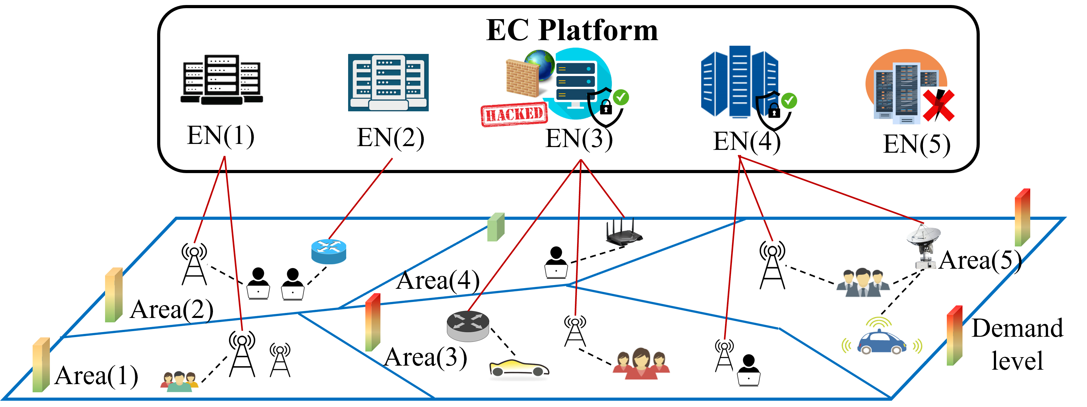
Figure 1: System model

The operation of the edge network can be disrupted for various reasons. To account for this, we consider the presence of a hypothetical intelligent adversary, i.e., an attacker, whose objective is to cause maximum damage to the edge system performance given its limited attack resources. The EC platform acts as the defender. We assume the attacker has complete knowledge of the optimal operation plan of the platform. This is a reasonable assumption as the defender would not be worse off even if the attacker possesses a less-than-perfect model of the defender’s system or fails to execute a perfect attack plan.

When an EN fails due to any reason, we consider it as being attacked by the hypothetical attacker. The workload initially assigned to the failed EN must be reallocated to the remaining active ENs. The survivability of the system against edge failures can be achieved through EN protection. We assume that the EC platform has a certain budget for EN hardening, and the maximum number of ENs that can be protected is represented by $K$. Then, the platform can optimize the EN protection decision by viewing this problem through the lens of an attacker who can only successfully attack at most $K$ simultaneous ENs. Obviously, $K\leq|\mathcal{N}|=N$.

Since the exact node failures can not be predicted accurately at the time of making the protection decision, we propose techniques to search for optimal disruptive attacks, given the posited offensive resources of the attacker. To this end, we formulate a bilevel optimization problem where the defender solves the inner problem to minimize the impact on user experience, while the attacker solves the outer problem to maximize the degradation of system performance. The solution to this problem yields the most disruptive attack that the attacker could undertake, as well as the critical ENs that should be reinforced for optimal protection.

II-B EC Platform Optimization Model

First, we present the optimal operating model for the EC platform under normal conditions without attack. The platform’s objective is to improve the user experience by reducing the overall delay and the extent of unmet demand. Hence, it needs to solve the following optimization problem:

$$\textbf{(D)}~{}~{}\min_{{\mathbf{x}},{\mathbf{q}}}~{} (1-\gamma)\sum_{i}\phi_{i}q_{i}+\gamma\sum_{i,j}d_{i,j}x_{i,j}$$ (1a)

s.t. $$\sum_{i}x_{i,j}\leq C_{j},~{}\forall j$$ (1b)

$$\sum_{j}x_{i,j}+q_{i}=\lambda_{i},~{}\forall i;~{}x_{i,j}\leq C_{j}a_{i,j},~{}\forall i,j$$ (1c)

$$\frac{q_{i}}{\lambda_{i}}\leq\theta,~{}\forall i;~{}~{}\Bigg{|}\frac{q_{i}}{\lambda_{i}}-\frac{q_{i^{\prime}}}{\lambda_{i^{\prime}}}\Bigg{|}\leq\beta,~{}\forall i,i^{\prime}$$ (1d)

$$x_{i,j}\geq 0,~{}\forall i,j,~{}~{}q_{i}\geq 0,~{}\forall i.$$ (1e)

The first term in the objective function (1a) captures the total penalty for unmet demand. The second term represents the delay penalty. The weighing factor $\gamma$ can be used by the EC platform to express its priorities towards reducing the delay and the unmet demand. Overall, the EC platform aims to minimize the weighted sum of the unmet demand penalty and the delay penalty. The computing resource capacity constraints are presented in (1b), which shows that the total amount of workload allocated to EN $j$ can not exceed its capacity. The workload allocation constraints (1c) indicate the demand from each area must be either served by some ENs or dropped.

Since we focus on delay-sensitive services, constraints (1c) also impose that the demand from each area can only be served by a subset of ENs which are sufficiently close to that area. We use $a_{i,j}$ as a binary indicator to denote if EN $j$ satisfies the prerequisites for serving the demand from area $i$. In particular, if $a_{i,j}=0$, then $x_{i,j}=0$, i.e., EN $j$ is not eligible to serve the demand from area $i$. Otherwise, the workload assigned from area $i$ to EN $j$ should not exceed the capacity $C_{j}$ of the EN.

For quality control, the EC platform can enforce that the ratio of the unmet demand to the total demand in each area $i$ should not exceed a given threshold $\theta$ as shown in (1d). This condition ensures that each area is allocated sufficient resources for operating critical services in case of disruption. Constraints (1d) enforces a soft fairness condition among different areas in terms of the proportions of unmet demand. Specifically, the proportions of unmet demand between any two areas should not differ more than a certain threshold $\beta$.

II-C Attacker-Defender Model

We are now ready to describe the attacker-defender model to determine the set of critical ENs. The attacker can use this model to find an optimal attack plan, given its limited offensive resources, to maximally degrades the performance of the EC platform during disruptions by increasing the total amount of unmet demand as well as the overall network delay By studying attack strategies through the lens of the attacker, it helps us understand how to make the edge network less vulnerable. In our model, the EC platform acts as the defender.

Let $z_{j}$ be a binary variable that takes the value of $1$ if EN $j$ is successfully attacked by the attacker. For simplicity, we assume that an EN will completely fail if it is attacked. Denote an attack plan of the attacker by ${\mathbf{z}}=(z_{1},\cdots,z_{N})$ $\in\mathcal{Z}$, where $\mathcal{Z}$ is the set of all possible attack plans that can be carried out by the attacker. In other words, $\mathcal{Z}$ is the set of the attacker’s options to interdict different combinations of ENs in the network. A natural form of set $\mathcal{Z}$ is:

$$\mathcal{Z}=\Big{\{}{\mathbf{z}}\in\{0,1\}^{N}:~{}\sum_{j}z_{j}\leq K\Big{\}},$$ (2)

where $K$ is the maximum number of ENs that the attacker can attack simultaneously. Note that our proposed model and solution can easily deal with a more general (polyhedral) form of set $\mathcal{Z}$. Overall, the attacker-defender model can be expressed as a max-min optimization problem as follows:

$$\textbf{(AD)}~{}~{}\max_{{\mathbf{z}}\in\mathcal{Z}}~{}\min_{{\mathbf{x}},{\mathbf{q}}\in\mathcal{S}({\mathbf{z}})}~{}(1-\gamma)\sum_{i}\phi_{i}q_{i}+\gamma\sum_{i,j}d_{i,j}x_{i,j},$$ (3)

where $\mathcal{S}({\mathbf{z}})$ represents the defender’s set of feasible actions, restricted by the attack plan ${\mathbf{z}}$. Concretely, $\mathcal{S}({\mathbf{z}})$ captures all the operational constraints of the defender during an attack. Since attacked ENs cannot serve any demand, constraints (1b) need to be modified as follows:

$$\sum_{i}x_{i,j}\leq C_{j}(1-z_{j}),\quad\forall j.$$ (4)

It can be seen that if EN $j$ fails (i.e., $z_{j}=1$), then (4) implies $\sum_{i}x_{i,j}=0$, thus, $x_{i,j}=0,~{}\forall i,j$, and EN $j$ is unable to serve any user requests. Since (4) already enforces $x_{i,j}=0,~{}\forall i,j$, when $z_{j}=1$, we do not need to modify (1c). Hence, the feasible set $\mathcal{S}({\mathbf{z}})$ given the attack plan ${\mathbf{z}}$ can be given as:

$$\mathcal{S}({\mathbf{z}})=\Big{\{}{\mathbf{x}},{\mathbf{q}}:~{}\eqref{eq-const:WorkloadAllocation}-\eqref{eq-const:vars},~{}\eqref{eq-const:CapacityA}\Big{\}}.$$ (5)

The attacker-defender model (3) aims to find a critical set of ENs by identifying a maximally disruptive resource-constrained attack that an attacker might undertake. The inner minimization problem in (3) represents the optimal operation model of the EC platform (i.e., the defender) under a specific attack plan ${\mathbf{z}}$. The outer maximization problem models the attacker’s objective to incur the highest cost to the EC platform during the attack. The solutions obtained from solving the optimal-attack problem (3) suggest the set of $K$-critical ENs to be protected to maximize the user experience.

The attacker-defender problem (AD) in (3) is a challenging bilevel program [15]. Refer to Appendix A in [16] for the bilevel formulation. The computational difficulty stems from the max-min structure of the problem. The outer problem also referred to as the leader problem, represents the attacker problem that seeks to maximize the defender’s loss caused by the disruption. The inner minimization problem, also referred to as the follower problem, captures the optimal operation of the edge platform under a specific attack plan ${\mathbf{z}}$. The platform aims to optimally allocate the workload to non-attacked ENs to mitigate the impact of attacks by minimizing the amount of unmet demand as well as the overall network delay.

III Solution Approach

To solve the problem (3), we first convert the inner problem into a linear program (LP) for a fixed value of ${\mathbf{z}}$. Then, (3) becomes a bilevel LP with binary variables in the upper level, which imposes difficulties [15]. We propose transforming the inner minimization problem into a maximization problem by relying on LP duality. Consequently, the max-min problem (3) can now be reformulated as a max-max problem, which is simply a maximization problem. The resulting maximization problem is a mixed-integer nonlinear program (MINLP) containing several bilinear terms. By linearizing the bilinear terms, we can convert the MINLP into an MILP that can be solved by off-the-shelf solvers. The detailed solution is described below.

First, given a fixed attack plan ${\mathbf{z}}$, the inner minimization problem in (3) can be rewritten as an equivalent LP below:

$$\min_{{\mathbf{x}},{\mathbf{q}}}\quad (1-\gamma)\sum_{i}\phi_{i}q_{i}+\gamma\sum_{i,j}d_{i,j}x_{i,j}$$ (6a)

s.t. $$\sum_{i}x_{i,j}\leq C_{j}(1-z_{j}),~{}\forall j~{} (\pi_{j})$$ (6b)

$$\sum_{j}x_{i,j}+q_{i}=\lambda_{i},~{}\forall i~{} (\mu_{i})$$ (6c)

$$x_{i,j}\leq C_{j}a_{i,j},~{}\forall i,j (\sigma_{i,j})$$ (6d)

$$\frac{q_{i}}{\lambda_{i}}-\frac{q_{i^{\prime}}}{\lambda_{i^{\prime}}}\leq\beta,~{}\forall i,i^{\prime} (\eta_{i,i^{\prime}})$$ (6e)

$$\frac{q_{i}}{\lambda_{i}}-\frac{q_{i^{\prime}}}{\lambda_{i^{\prime}}}\geq-\beta,~{}\forall i,i^{\prime} (\tau_{i,i^{\prime}})$$ (6f)

$$x_{i,j}\geq 0,\forall i,j;~{}q_{i}\geq 0,\forall i;~{}\frac{q_{i}}{\lambda_{i}}\leq\theta,\forall i (\nu_{i})$$ (6g)

$\pi_{j},\mu_{i},\sigma_{i,j},\eta_{i,i^{\prime}},\tau_{i,i^{\prime}},\nu_{i}$ are the dual variables associated with constraints (6b)-(6g), respectively.

To transform the max-min bilevel program into a single-level problem, a common approach is to utilize the Karush–Kuhn–Tucker (KKT) conditions to convert the inner follower problem into a set of linear constraints (see Appendix B in our technical report [16]). However, this solution is not computationally efficient because the reformulated single-level optimization problem contains a large number of complimentary constraints. Instead, we employ the LP duality to convert the minimization problem (6a)-(6g) to the following equivalent maximization problem.

$$\max_{\pi,\sigma,\mu,\eta,\tau,\nu}-\!\sum_{j}\!C_{j}(1\!-\!z_{j})\pi_{j}\!+\!\sum_{i}\!\lambda_{i}\mu_{i}\!-\!\sum_{i,j}\!C_{j}a_{i,j}\sigma_{i,j}$$

$$-\sum_{i}\sum_{i^{\prime}=i+1}^{M}\beta(\eta_{i,i^{\prime}}+\tau_{i,i^{\prime}})-\sum_{i}\theta\nu_{i}$$ (7a)

$$\text{s.t.}\quad\quad\quad\quad\quad\quad-\pi_{j}+\mu_{i}-\sigma_{i,j}\leq\gamma d_{i,j},~{}\forall i,j$$ (7b)

$$\mu_{i}-\frac{1}{\lambda_{i}}\sum_{l=i+1}^{M}\left(\eta_{i,l}-\tau_{i,l}\right)+\frac{1}{\lambda_{i}}\sum_{l=1}^{i-1}\left(\eta_{l,i}-\tau_{l,i}\right)-\dfrac{\nu_{i}}{\lambda_{i}}$$

$$\leq(1-\gamma)\phi_{i},~{}\forall i$$ (7c)

$$\pi_{j}\geq 0,\sigma_{i,j}\geq 0,\eta_{i,i^{\prime}}\geq 0,\tau_{i,i^{\prime}}\geq 0,\nu_{i}\geq 0,~{}\forall i,i^{\prime},j.$$ (7d)

The bilinear term $(1-z_{j})\pi_{j}$ in (7) is a product of a continuous variable and a binary variable. To tackle this, we define a new auxiliary non-negative continuous variable $g_{j}$, where $g_{j}=(1-z_{j})\pi_{j},~{}\forall j$. The constraint $g_{j}=(1-z_{j})\pi_{j}$ can be implemented equivalently through the following linear inequalities:

$$g_{j}\leq M_{j}(1-z_{j}),~{}~{}g_{j}\leq\pi_{j} ,~{}\forall j$$ (8a)

$$g_{j}\geq 0,~{}~{}g_{j}\geq\pi_{j}-M_{j}z_{j} ,~{}\forall j,$$ (8b)

where each $M_{j}$ is a sufficiently large number. Based on the linearization steps above, we obtain an MILP that is equivalent to the attacker-defender problem (3), as follows:

$$\max_{{\mathbf{z}},{\mathbf{g}},\pi,\sigma,\mu,\eta,\tau,\nu} \!\!\!-\!\sum_{j}\!C_{j}g_{j}\!+\!\sum_{i}\!\lambda_{i}\mu_{i}\!-\!\sum_{i,j}\!C_{j}a_{i,j}\sigma_{i,j}$$ (9a)

$$\!\!\!\!\!\!-\sum_{i}\sum_{i^{\prime}=i+1}^{M}\beta(\eta_{i,i^{\prime}}+\tau_{i,i^{\prime}})-\sum_{i}\theta\nu_{i}$$ (9b)

s.t. $$\!\!\!\eqref{eq-const:Duality1}-\eqref{eq-const:Duality4};\sum_{j}z_{j}\leq K;z_{j}\in\{0,1\},\forall j.$$ (9c)

This MILP problem can now be solved efficiently by MILP solvers such as Gurobi, CPLEX, and Mosek. Table I compares the number of constraints and variables between duality- and KKT- based reformulations. The duality reformulation has a simpler structure and fewer variables and constraints and is usually less computationally expensive. Another disadvantage of the KKT-based method lies in the weak relaxation of the big-M method, which can greatly affect the running time.

	KKT	Duality
# constraints	$5N+M(8M+8N+1)$	$6N+2M(M+N)$
# variables ($\mathbb{Z}$)	$2N+2M(M+N)$	$N$
# variables ($\mathbb{R}$)	$N+2M(M+N+1)$	$2N+M(2M+N)$

TABLE I: KKT-based vs duality-based reformulations

IV Numerical Results

Similar to [1, 3, 2], we adopt the Barabasi-Albert model to generate a random scale-free edge network topology with $100$ nodes and the attachment rate of $2$ [1]. The link delay between each pair of nodes is generated randomly in the range of [2, 5] ms. The network delay between any two nodes is the delay of the shortest path between them [2]. From the generated topology, 80 nodes are chosen as APs and 30 nodes are chosen as ENs for our performance evaluation (i.e., $M=80$, $N=30$). Also, $a_{i,j}$ is set to be 1 if $d_{i,j}$ is less than $20$ ms. The capacity $C_{j}$ of each EN $j$ is randomly selected from the set $\{16,32,64,128,256,512,1024\}$ vCPUs. The resource demand (i.e., workload) in each area is randomly drawn in the range of [20, 35] vCPUs [2]. The penalty for each unit of unmet demand is set to be 5 $/vCPU (i.e., $\phi_{i}=5,~{}\forall i$). The EC platform can adjust $\gamma$ to control the trade-off between the unmet demand and the overall network delay. A smaller value of $\gamma$ implies the platform gives more priority to unmet demand mitigation than to delay reduction. For illustration purposes, we set $\gamma$ to be $0.1$. Also, $\theta$ is set to be 0.8.

We first evaluate the performance of the proposed model and three benchmark schemes, including: (i) No hardening: proactive EN protection is not considered; (ii) Heuristic: the system protects $K$ ENs with highest computing capacities; and (iii) Random: a random protection plan within the protection budget, i.e., protecting $K$ ENs at random. The simulation is conducted for different values of $K$ and the number of actual EN failures. We run each scheme to obtain a set of ENs to be protected. For our proposed model, we solve (3) to obtain the set of $K$ critical ENs. This set and the set of actual EN failures are then used as an input to problem (6a)-(6g) to compute the actual total cost of the platform. For each experiment, we randomly generate $500$ scenarios of actual EN failures and compute both average and worst-case performance.

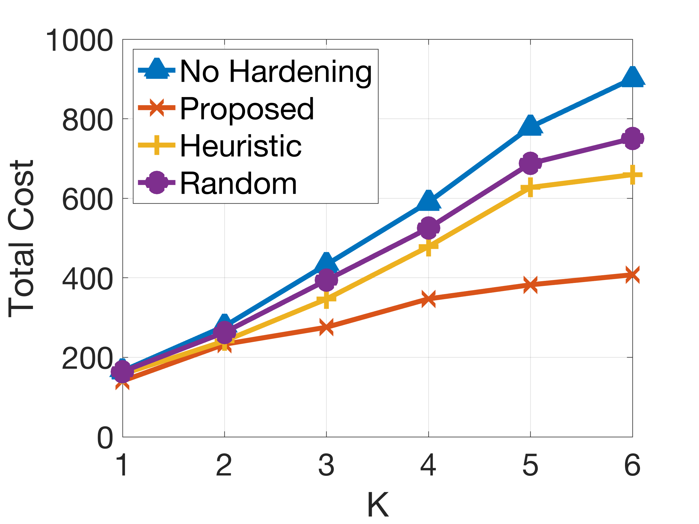
(a) Average Cost

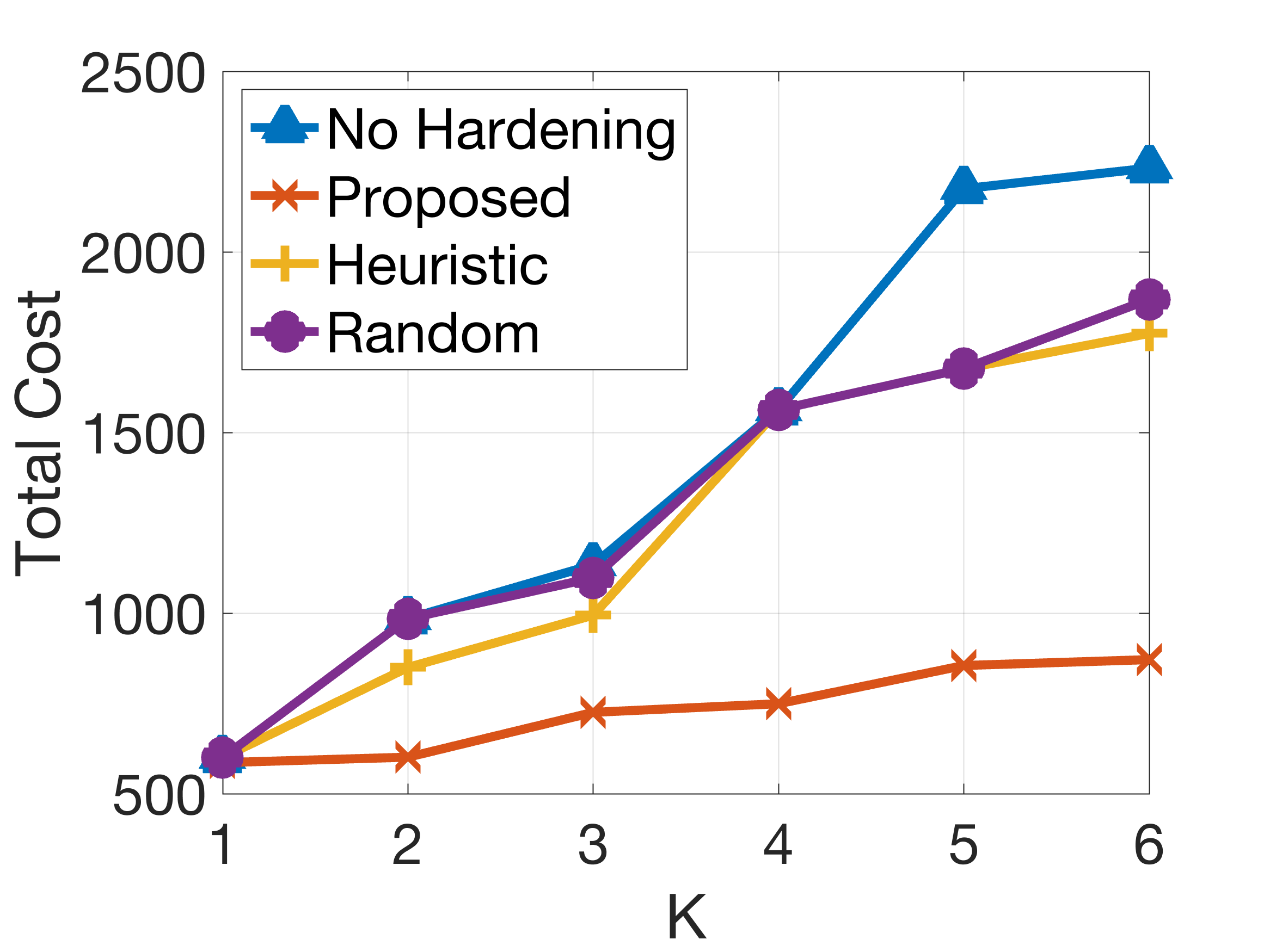
(b) Worst-case Cost

Figure 2: Performance comparison

Fig. 2 compares the performance of the four hardening schemes when the actual number of failures equals the defense budget $K$. Among the total of $N=30$ ENs, we vary the number of EN failures $K$ from 1 to 6. As expected, “No Hardening” results in the highest cost for every value of $K$, as all ENs are susceptible to attacks and the attacker has more flexibility to target the critical ENs that cause the greatest disruption. In contrast, the attacker has more limited options with EN protection considered in the other schemes. The proposed scheme significantly outperforms the other schemes. Also, for every scheme, the total cost increases as $K$ increases since there are fewer surviving ENs to serve the demand.

Fig. 3 illustrates the benefit of proactive EN hardening using our model by showing the effect of having different numbers of protected ENs during the planning stage for different attack/failure scenarios. The performance for different numbers of protected ENs ($K$) and the actual number of EN failures ($Q$) are examined. Each curve in the figure corresponds to a given value of $Q$. We can easily see that the total cost increases as $Q$ increases. More interestingly, the defender can drastically reduce its cost by protecting just a few ENs. For example, protecting only one or two ENs results in a significantly lower total cost compared to the case without any protection. Thus, proactive EN protection is beneficial even when the number of actual failures is larger than the defense budget.

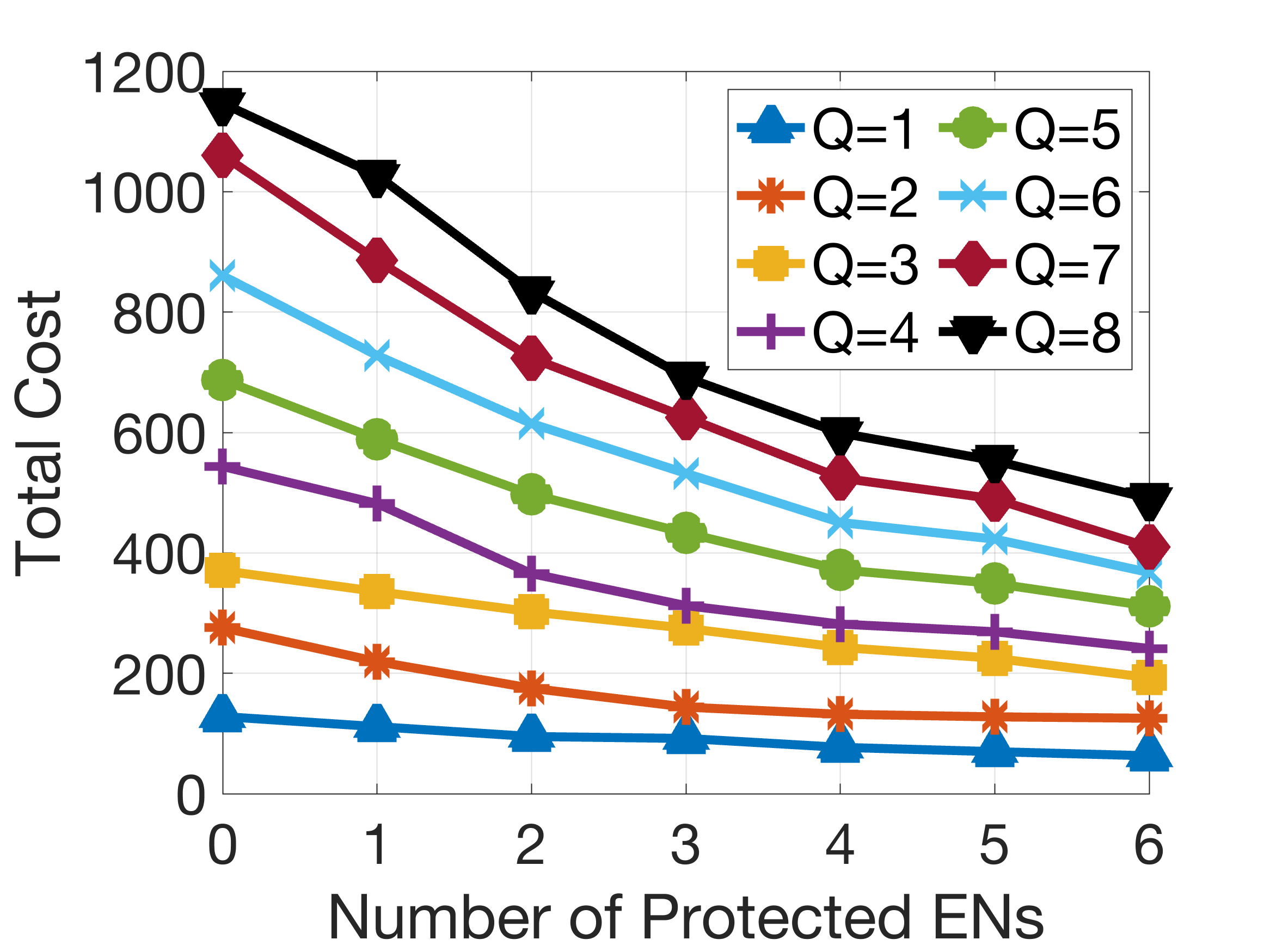
(a) Average Cost

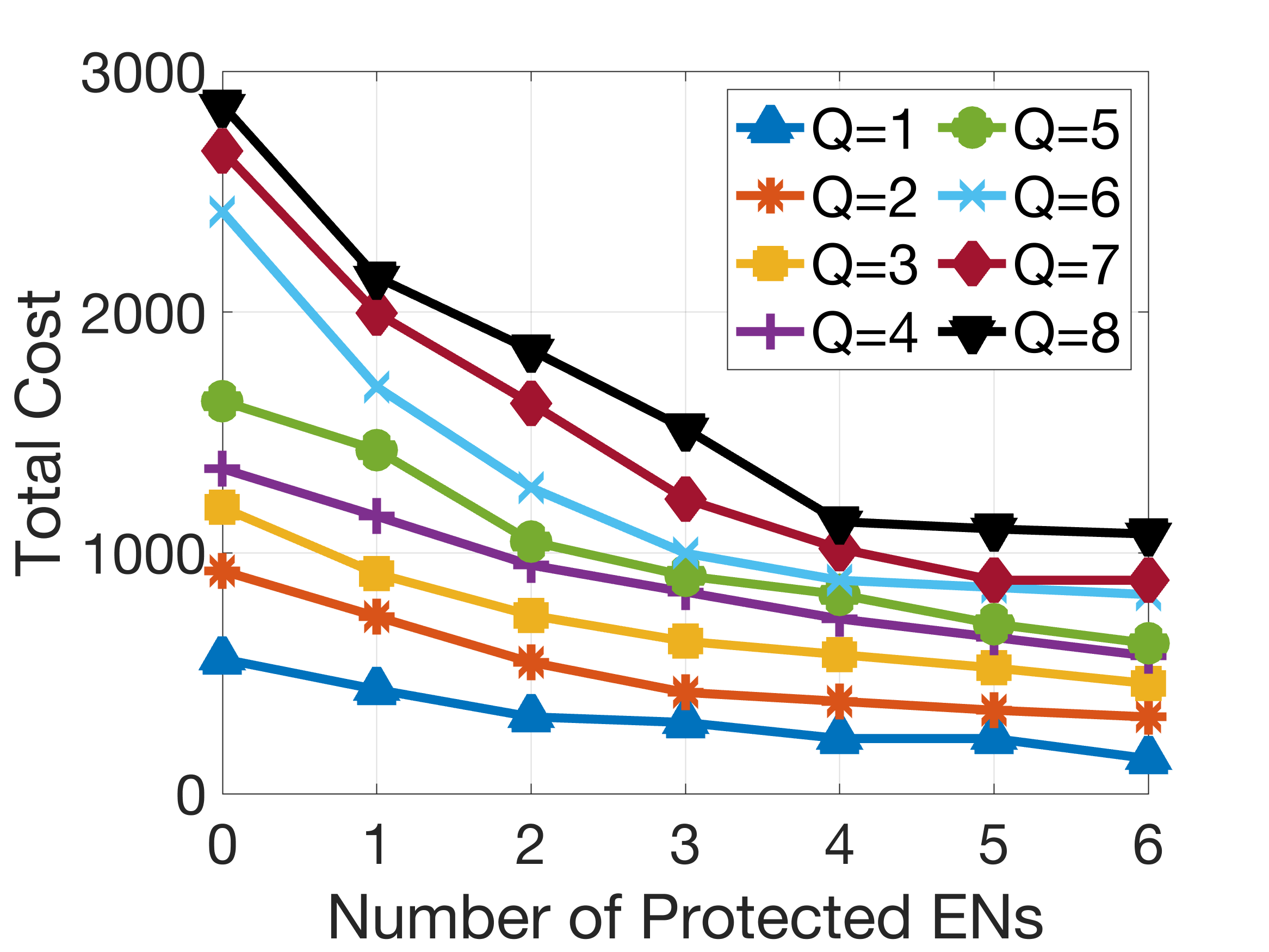
(b) Worst-case Cost

Figure 3: Impacts of proactive EN protection on the total cost

(a) $\beta=0.2$

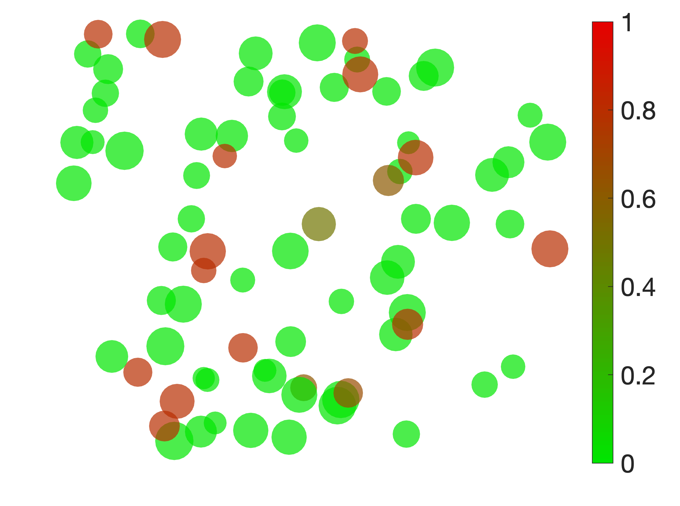
(b) $\beta=0.8$

Figure 4: The proportions of unmet demands in different areas

Fig. 4 shows the impact of fairness consideration. A lower value of $\beta$ implies that the platform cares more about fairness during disruptions. When the fairness condition is relaxed, i.e, larger values of $\beta$ (e.g., $\beta=0.8$ in Fig. 4(b)), there are some areas with particularly high rates of dropped requests (i.e., higher unmet demand). On the other hand, when the fairness condition is strictly imposed (e.g., $\beta=0.2$ in Fig. 4(a)), all the areas have comparable proportions of unmet demand.

	$\beta=0.2$	$\beta=0.8$
$K=2$	$\{24,26\}$	$\{24,26\}$
$K=4$	$\{2,11,15,21\}$	$\{2,10,24,26\}$
$K=6$	$\{2,11,15,21,23,26\}$	$\{2,5,10,24,25,26\}$

TABLE II: The set of critical ENs

Table II presents the critical EN sets for $\beta$ values of $0.2$ and $0.8$. The sets are found to be significantly different, with a varying degree of fairness consideration. When the fairness constraint is less stringent (i.e., $\beta=0.8$), the set tends to consist of ENs with high capacity. However, when the fairness constraint is more stringent (i.e., $\beta=0.2$), the set tends to comprise ENs with smaller capacities that have more potential to serve requests from more areas (i.e., close to more areas). The resource allocation decision during disruption can also differ, even if the sets of critical ENs are the same. Indeed, there is an inherent trade-off between fairness and cost, as depicted in Fig. 5. Finally, Table III compares the running time of the KKT-based and duality-based reformulations. It should be noted that all the experiments were conducted on an M1 MacBook Air with 3.2 GHz processor and 8 GB RAM. On high-performance computing servers, the actual running time can be significantly faster.

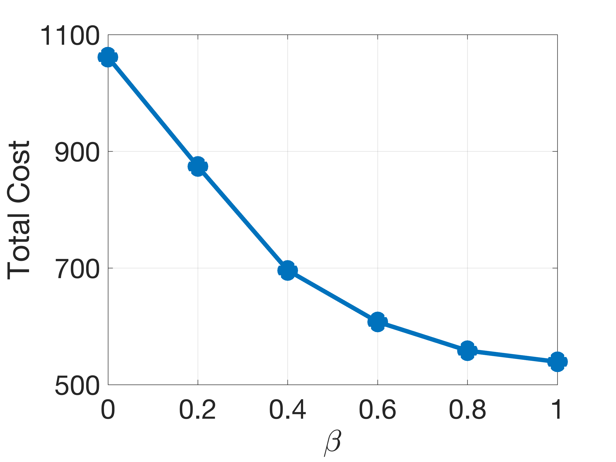
Figure 5: Total penalty for different values of $\beta$

	KKT (seconds)	Duality (seconds)
$N=10,M=30$	$15.5208$	$2.9579$
$N=30,M=80$	$235.0888$	$7.8576$
$N=80,M=100$	$4359.9689$	$27.1822$
$N=200,~{}M=1000$	N/A	$18599.8247$

TABLE III: Computational time comparison

V Conclusion

This letter introduced a novel fairness-aware robust model to help a budget-constrained EC platform determine the critical ENs to be safeguarded against possible disruptions. The model incorporates the coordination of both hardening and resource allocation decisions in order to enhance system resilience and service quality while striking a balance between fairness and system efficiency. For future research, it is intended to integrate multiple uncertainties, as well as multiple services and resource types into the proposed framework. Exploring the impact of proactive defense through a multi-faceted defender-attacker-defender model is another interesting direction.

-A The Bilevel Attacker-Defender Optimization Problem

(AD) $$\max_{{\mathbf{z}}}~{}(1-\gamma)\sum_{i}\phi_{i}q_{i}+\gamma\sum_{i,j}d_{i,j}x_{i,j}$$

subject to $$\sum_{j}z_{j}\leq K;~{}~{}z_{j}\in\{0,~{}1\},\quad\forall j$$

$${\mathbf{x}},{\mathbf{q}}\in\operatornamewithlimits{argmin}_{{\mathbf{x}},{\mathbf{q}}}\Bigg{\{}(1-\gamma)\sum_{i}\phi_{i}q_{i}+\gamma\sum_{i,j}d_{i,j}x_{i,j}$$

$$\text{subject to}~{}~{}~{}\sum_{i}x_{i,j}\leq C_{j}(1-z_{j}),~{}\forall j$$

$$\qquad\qquad\quad\sum_{j}x_{i,j}+q_{i}=\lambda_{i},~{}\forall i$$

$$\qquad\qquad\quad 0\leq x_{i,j}\leq C_{j}a_{i,j},~{}\forall i,j$$

$$\qquad\qquad\quad 0\leq\frac{q_{i}}{\lambda_{i}}\leq\theta,~{}\forall i$$

$$\qquad\qquad\quad\Bigg{|}\frac{q_{i}}{\lambda_{i}}-\frac{q_{i^{\prime}}}{\lambda_{i^{\prime}}}\Bigg{|}\leq\beta,~{}\forall i,~{}i^{\prime}\Bigg{\}}.$$

-B KKT-based Solution

The Lagrangian function of the inner minimization problem (6a)-(6g) in the subproblem (SP) is:

$$\allowdisplaybreaks[2]\mathcal{L}({\mathbf{x}},{\mathbf{q}},\pi_{j},\mu_{i},\sigma_{i,j},\eta_{i,i^{\prime}},\tau_{i,i^{\prime}},\nu_{i},\xi_{i,j},\rho_{i})=-\sum_{i,j}\!\xi_{i,j}x_{i,j}$$

$$-\sum_{i}\!\rho_{i}q_{i}+(1-\gamma)\sum_{i}\phi_{i}q_{i}+\gamma\sum_{i,j}d_{i,j}x_{i,j}$$

$$+\!\sum_{j}\pi_{j}\Big{(}\!\sum_{i}x_{i,j}-\!C_{j}(1-z_{j})\!\Big{)}\!+\!\sum_{i}\mu_{i}\Big{(}\sum_{j}x_{i,j}+q_{i}-\lambda_{i}\!\Big{)}$$

$$+\sum_{i,j}\sigma_{i,j}\Big{(}x_{i,j}-C_{j}a_{i,j}\Big{)}+\sum_{i}\nu_{i}\Big{(}\frac{q_{i}}{\lambda_{i}}-\theta\!\Big{)}$$

$$+\sum_{i,i^{\prime}}\eta_{i,i^{\prime}}\Big{(}\frac{q_{i}}{\lambda_{i}}-\frac{q_{i^{\prime}}}{\lambda_{i^{\prime}}}-\beta\Big{)}-\sum_{i,i^{\prime}}\tau_{i,i^{\prime}}\Big{(}\frac{q_{i}}{\lambda_{i}}-\frac{q_{i^{\prime}}}{\lambda_{i^{\prime}}}+\beta\Big{)}.$$

The KKT conditions give

$$\frac{\partial\mathcal{L}}{\partial x_{i,j}}=\gamma d_{i,j}+\pi_{j}+\mu_{i}+\sigma_{i,j}-\xi_{i,j}=0 ,~{}\forall i,j$$ (12a)

$$\frac{\partial\mathcal{L}}{\partial q_{i}}=(1-\gamma)\phi_{i}+\mu_{i}+\frac{1}{\lambda_{i}}\!\sum_{l=i+1}^{M}\!\left(\eta_{i,l}-\tau_{i,l}\right)~{}~{}$$ (12b)

$$-\frac{1}{\lambda_{i}}\sum_{l=1}^{i-1}\!\left(\eta_{l,i}-\tau_{l,i}\right)+\frac{\nu_{i}}{\lambda_{i}}-\rho_{i}=0 ,~{}\forall i$$ (12c)

$$0\leq\pi_{j}~{}\bot~{}C_{j}(1-z_{j})-\sum_{i}x_{i,j}\geq 0 ,~{}\forall j$$ (12d)

$$\sum_{j}x_{i,j}+q_{i}=\lambda_{i} ,~{}\forall j$$ (12e)

$$0\leq\sigma_{i,j}~{}\bot~{}C_{j}a_{i,j}-x_{i,j}\geq 0 ,~{}\forall j$$ (12f)

$$0\leq\nu_{i}~{}\bot~{}\theta-\frac{q_{i}}{\lambda_{i}}\geq 0 ,~{}\forall i,j$$ (12g)

$$0\leq\xi_{i,j}~{}\bot~{}x_{i,j}\geq 0 ,~{}\forall i,j$$ (12h)

$$0\leq\rho_{i}~{}\bot~{}q_{i}\geq 0 ,~{}\forall i$$ (12i)

where (12a)-(12b) are the stationary conditions, (12d)-(12i) are the primal feasibility, dual feasibility and complementary slackness conditions. From (12a)-(12b), we have:

$$\gamma d_{i,j}+\pi_{j}+\mu_{i}+\sigma_{i,j} =\xi_{i,j} ,~{}\forall i,j$$ (13)

$$(1-\gamma)\phi_{i}+\mu_{i}+\frac{1}{\lambda_{i}}\sum_{l=i+1}^{M}\left(\eta_{i,l}-\tau_{i,l}\right)$$ (14)

$$-\frac{1}{\lambda_{i}}\sum_{l=1}^{i-1}\left(\eta_{l,i}-\tau_{l,i}\right)+\frac{\nu_{i}}{\lambda_{i}} =\rho_{i} ,~{}\forall i.$$ (15)

Moreover, from (12h), if $x_{i,j}>0$, then $\xi_{i,j}=0$ and (13) implies that $\gamma d_{i,j}+\pi_{j}+\sigma_{i,j}+\mu_{i}=0,~{}\forall i,j.$ Thus,

$$\Big{(}\gamma d_{i,j}+\pi_{j}+\sigma_{i,j}+\mu_{i}\Big{)}x_{i,j}=0,~{}\forall i,j.$$ (16)

Similarly, we have

$$\Bigg{[}(1-\gamma)\phi_{i}+\mu_{i}+\frac{1}{\lambda_{i}}\sum_{l=i+1}^{M}\left(\eta_{i,l}-\tau_{i,l}\right)$$ (17)

$$-\frac{1}{\lambda_{i}}\sum_{l=1}^{i-1}\left(\eta_{l,i}-\tau_{l,i}\right)+\frac{\nu_{i}}{\lambda_{i}}\Bigg{]}q_{i} =0,~{}\forall i.$$ (18)

Therefore, the conditions (12h)-(15) are equivalent to the following set of constraints:

$$0\leq\gamma d_{i,j}+\pi_{j}+\mu_{i}+\sigma_{i,j}~{}\bot~{}x_{i,j}\geq 0 ,~{}\forall i,j$$ (19a)

$$0\leq(1-\gamma)\phi_{i}+\mu_{i}+\frac{1}{\lambda_{i}}\sum_{l=i+1}^{M}\left(\eta_{i,l}-\tau_{i,l}\right)~{}~{}~{}~{}$$ (19b)

$$-\frac{1}{\lambda_{i}}\sum_{l=1}^{i-1}\left(\eta_{l,i}-\tau_{l,i}\right)+\frac{\nu_{i}}{\lambda_{i}}~{}\bot~{}q_{i}\geq 0 ,~{}\forall i.$$ (19c)

It is worth noting that we can directly use the set of KKT conditions (13)-(15) to solve the subproblem, but it will involve more variables (i.e., $\xi$ and $\rho$) compared to solving the subproblem with (19a)-(19b). In brief, based on the Karush–Kuhn–Tucker (KKT) conditions above, the (AD) problem (3) is equivalent to the following problem with complementary constraints:

$$\max_{{\mathbf{x}},{\mathbf{q}},{\mathbf{z}},\pi,\sigma,\mu,\eta,\tau,\nu} (1-\gamma)\sum_{i}\phi_{i}q_{i}+\gamma\sum_{i,j}d_{i,j}x_{i,j}$$ (20a)

subject to $$\eqref{eq:kktcs1},\eqref{eq:kktcs3},\eqref{eq:kktcs2},\eqref{eq:kktcs4},\eqref{eq:kktxijex},\eqref{eq:kktuiex}$$ (20b)

$$z_{j}\in\{0,1\},~{}\forall j,~{}~{}\sum_{j}z_{j}\leq K,$$ (20c)

where the last constraints in (20c) represents the set of feasible attack plans $\mathcal{Z}$.

The Complete MILP Formulation Note that a complimentary constraint $0\leq x\bot\pi\geq 0$ means $x\geq 0,\pi\geq$ and $x.\pi=0$. Thus, it is a nonlinear constraint. However, this nonlinear complimentary constraint can be transformed into equivalent exact linear constraints by using the Fortuny-Amat transformation. Specifically, the complementarity condition $0\leq x\bot\pi\geq 0$ is equivalent to the following set of mixed-integer linear constraints:

$$x\geq 0;~{}~{}x\leq(1-u)M$$ (21a)

$$\pi\geq 0;~{}~{}\pi\leq uM,~{}~{}u\in\{0;1\},$$ (21b)

where M is a sufficiently large constant. By applying this transformation to all the complementary constraints listed in (20b), we obtain an MILP that is equivalent to the problem (3). The explicit form of this MILP is as follows:

$$\max_{{\mathbf{x}},{\mathbf{q}},{\mathbf{z}},\pi,\sigma,\mu,\eta,\tau,\nu,{\mathbf{u}}}(1-\gamma)\sum_{i}\phi_{i}q_{i}~{}+ \!\!\!\!\!\!\!\!\!\!\!\!\!\!\gamma\sum_{i,j}d_{i,j}x_{i,j}$$ (22a)

subject to

$$0\leq\gamma d_{i,j}+\pi_{j}+\mu_{i}+\sigma_{i,j}\leq u_{i,j}^{0}M_{i,j}^{0} ,\forall i,j$$ (22b)

$$0\leq x_{i,j}\leq(1-u_{i,j}^{0})M_{i,j}^{0} ,\forall i,j$$ (22c)

$$0\leq(1-\gamma)\phi_{i}+\mu_{i}+\frac{1}{\lambda_{i}}\sum_{l=i+1}^{M}\left(\eta_{i,l}-\tau_{i,l}\right)$$ (22d)

$$~{}~{}~{}~{}-\frac{1}{\lambda_{i}}\sum_{l=1}^{i-1}\left(\eta_{l,i}-\tau_{l,i}\right)+\frac{\nu_{i}}{\lambda_{i}}\leq u_{i}^{1}M_{i}^{1} ,\forall i$$ (22e)

$$0\leq q_{i}\leq(1-u_{i}^{1})M_{i}^{1} ,\forall i$$ (22f)

$$0\leq C_{j}(1-z_{j})-\sum_{i}x_{i,j}\leq u_{j}^{2}M_{j}^{2} ,\forall j$$ (22g)

$$0\leq\pi_{j}\leq(1-u_{j}^{2})M_{j}^{2} ,\forall j$$ (22h)

$$0\leq C_{j}a_{i,j}-x_{i,j}\leq u_{i,j}^{3}M_{i,j}^{3} ,\forall i,j$$ (22i)

$$0\leq\sigma_{i,j}\leq(1-u_{i,j}^{3})M_{i,j}^{3} ,\forall i,j$$ (22j)

$$0\leq\beta-\frac{q_{i}}{\lambda_{i}}+\frac{q_{i^{\prime}}}{\lambda_{i^{\prime}}}\leq u_{i,i^{\prime}}^{4}M_{i,i^{\prime}}^{4} ,\forall i,i^{\prime}$$ (22k)

$$0\leq\eta_{i,i^{\prime}}\leq(1-u_{i,i^{\prime}}^{4})M_{i,i^{\prime}}^{4} ,\forall i,i^{\prime}$$ (22l)

$$0\leq\frac{q_{i}}{\lambda_{i}}-\frac{q_{i^{\prime}}}{\lambda_{i^{\prime}}}+\beta\leq u_{i,i^{\prime}}^{5}M_{i,i^{\prime}}^{5} ,\forall i,i^{\prime}$$ (22m)

$$0\leq\tau_{i,i^{\prime}}\leq(1-u_{i,i^{\prime}}^{5})M_{i,i^{\prime}}^{5} ,\forall i,i^{\prime}$$ (22n)

$$0\leq\theta-\frac{q_{i}}{\lambda_{i}}\leq u_{i}^{6}M_{i}^{6} ,\forall i$$ (22o)

$$0\leq\nu_{i}\leq(1-u_{i}^{6})M_{i}^{6} ,\forall i$$ (22p)

$$\sum_{j}x_{i,j}+q_{i}=\lambda_{i} ,\forall i$$ (22q)

$$u_{i,j}^{0},u_{i}^{1},u_{j}^{2},u_{i,j}^{3},u_{i,i^{\prime}}^{4},u_{i,i^{\prime}}^{5},u_{i}^{6}\in\{0,1\} ,\forall i,i^{\prime},j$$ (22r)

$$\sum_{j}z_{j}\leq K,~{}~{}z_{j}\in\{0,1\} ,\forall j$$ (22s)

where ${\mathbf{u}}$ represents the set of binary variables $u^{0},u^{1},u^{2}$, $u^{3},u^{4},u^{5},u^{6}$. Also, $M_{i,j}^{0},M_{i}^{1},M_{j}^{2},M_{i,j}^{3},M_{i,i^{\prime}}^{4},M_{i,i^{\prime}}^{5},M_{i}^{6}$ are sufficiently large numbers. The value of each $M$ should be large enough to ensure feasibility of the associated constraint. On the other hand, the value of each $M$ should not be too large to enhance the computational speed of the solver. Indeed, the value of each $M$ should be tighten to the limits of parameters and variables in the corresponding constraint.

-C Flowchart of the Proposed Solution Approach

The flow chart shown in Figure 6 summarizes the proposed system model and solution approach. Specifically, the inner minimization problem in (3) is first converted as a linear minimization program shown in (6). Then, by using strong duality in linear programming, (6) is equivalent to the non-linear maximization problem (7). At this step, the bilevel maxmin problem becomes a single-level non-linear maximization problem. The Fortuny-Amat transformation (big-M method) is then employed to convert bilinear constraints into equivalent sets of linear equations. Consequently, the initial bilevel problem (3) is transformed into a mixed-integer linear program (MILP) as shown in (9), which can be solved efficiently by off-the-shelf MILP solvers such as Gurobi, Mosek, Cplex. Note that instead of using LP strong duality theorem, we can also use KKT conditions to convert (6) into an equivalent set of linear equations. The KKT-based solution is presented in Appendix B. However, as explained, the KKT-based approach results in more integer variables and constraints in the MILP reformulation compared to that of the duality-based approach. The solution to the reformulated MILP problem is an optimal set of critical ENs that should be protected.

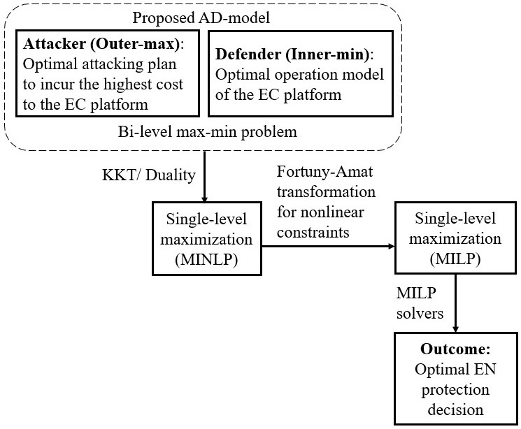
Figure 6: Flowchart of the solution approach

References

- [1] D. T. Nguyen, L. B. Le, and V. Bhargava, “Price-based resource allocation for edge computing: a market equilibrium approach,” IEEE Trans. Cloud Comput., vol. 9, no. 1, pp. 302–317, Jan.–Mar. 2021.
- [2] T. Nisha, D. T. Nguyen and V. K. Bhargava, “A Bilevel programming framework for joint edge resource management and pricing,” IEEE Internet Things J., vol. 9, no. 18, pp. 17280–17291, Sept. 2022.
- [3] D. T. Nguyen, H. T. Nguyen, N. Trieu, and V. K. Bhargava, “Two-stage robust edge service placement and sizing under demand uncertainty,” IEEE Internet Things J., vol. 9, no. 2, pp. 1560-1574, 15 Jan.15, 2022.
- [4] J. Cheng, D. T. Nguyen, and V. K. Bhargava, “Resilient edge service placement under demand and node failure uncertainties,” arXiv, 2022.
- [5] R. Roman, J. Lopez, and M. Mambo, “Mobile edge computing, fog et al.: A survey and analysis of security threats and challenges,” Future Gener. Comput. Syst., vol. 78, pp. 680–698, 2018.
- [6] H. Madsen, B. Burtschy, G. Albeanu, and F. Popentiu-Vladicescu, “Reliability in the utility computing era: Towards reliable fog computing,” in Proc. Int. Conf. Syst. Signals Image Process., pp. 43–46, 2013.
- [7] A. Aral and I. Brandic, “QoS channelling for latency sensitive edge applications,” in Proc. IEEE EDGE, pp. 166–173, 2017.
- [8] A. Aral and I. Brandic, “Learning spatio-temporal failure dependencies for resilient edge computing services,” IEEE Trans. Parallel Distrib. Syst., vol. 32, no. 7, pp. 1578–1590, Jul. 2021.
- [9] S. Liu, J. Yu, X. Deng and S. Wan, “FedCPF: An efficient-communication federated learning approach for vehicular edge computing in 6G communication networks,” IEEE Trans. Intell. Transp. Syst., vol. 23, no. 2, pp. 1616-1629, Feb. 2022
- [10] C. Wang, X. Wu, G. Liu, T. Deng, K. Peng and S. Wan, “Safeguarding cross-silo federated learning with local differential privacy,” Digital Commun. Net., vol. 8, pp. 446-454, 2022
- [11] R. Ford, A. Sridharan, R. Margolies, R. Jana, and S. Rangan, “Provisioning low latency, resilient mobile edge clouds for 5G,” in Proc. IEEE Conf. Comput. Commun. Workshops, May 2017, pp. 169–174.
- [12] Y. Qu, D. Lu, H. Dai, H. Tan, S. Tang, F. Wu, and C. Dong, “Resilient service provisioning for edge computing,” IEEE Internet Things J., 2021.
- [13] F. He and E. Oki, “Load balancing model against multiple controller failures in software defined networks,” in Proc. IEEE ICC, Dublin, Ireland, 2020.
- [14] M. Ito, F. He, and E. Oki, “Robust optimization for probabilistic protection with primary and backup allocations under uncertain demands”, in Proc. IEEE DRCN, pp. 1–6, 2021.
- [15] O. Ben-Ayed and C. E. Blair, “Computational difficulties of bilevel linear programming,” Oper. Res., vol. 38, no. 3, pp. 556–560, 1990.
- [16] Technical report, https://arxiv.org/pdf/2301.06644.pdf