gyre_tides: Modeling binary tides within the GYRE stellar oscillation code

Abstract

We describe new functionality in the GYRE stellar oscillation code for modeling tides in binary systems. Using a multipolar expansion in space and a Fourier-series expansion in time, we decompose the tidal potential into a superposition of partial tidal potentials. The equations governing the small-amplitude response of a spherical star to an individual partial potential are the linear, non-radial, non-adiabatic oscillation equations with an extra inhomogeneous forcing term. We introduce a new executable, gyre_tides, that directly solves these equations within the GYRE numerical framework. Applying this to selected problems, we find general agreement with results in the published literature but also uncover some differences between our direct solution methodology and the modal decomposition approach adopted by many authors.

In its present form gyre_tides can model equilibrium and dynamical tides of aligned binaries in which radiative diffusion dominates the tidal dissipation (typically, intermediate and high-mass stars on the main sequence). Milestones for future development include incorporation of other dissipation processes, spin-orbit misalignment, and the Coriolis force arising from rotation.

tablenum

1 Introduction

The GYRE stellar oscillation code (Townsend & Teitler, 2013; Townsend et al., 2018; Goldstein & Townsend, 2020) is a open-source software instrument that solves the linear, non-radial, non-adiabatic oscillation equations for an input stellar model. Released in 2013, it has been productively used to study of heat-driven oscillations in $\gamma$ Doradus and $\delta$ Scuti pulsators (e.g., Van Reeth et al., 2022; Murphy et al., 2022), slowly-pulsating B stars (e.g., Michielsen et al., 2021), variable sub-dwarf B stars (e.g. Silvotti et al., 2022), pulsating pre-main sequence stars (e.g., Steindl et al., 2021), DBV white dwarfs (e.g., Chidester et al., 2021), and hypothetical ‘dark’ stars (Rindler-Daller et al., 2021); to explore stochastically excited oscillations in solar-like, subgiant and red-giant stars (e.g., Nsamba et al., 2021; Li et al., 2020b, 2022); and to model oscillations of uncertain origin in red supergiant stars (Goldberg et al., 2020), post-outburst recurrent novae (Wolf et al., 2018) and even gas-giant planets (Mankovich et al., 2019).

This paper describes new functionality in GYRE for modeling static and dynamic tides in binary systems. The equations governing small tidal perturbations to one component of a binary are the linear oscillation equations with extra terms representing the gravitational forcing by the companion. Release 7.0 of GYRE implements these terms and the supporting infrastructure necessary to solve the tidal equations.

The view of astrophysical tides through the lens of forced oscillations was pioneered in a pair of seminal papers by Zahn (1970, 1975). These papers also introduce complementary approaches to solving the tidal equations, that we dub ‘modal decomposition’ (MD) and ‘direct solution’ (DS). In MD the tidal perturbations are decomposed as a superposition of the star’s free-oscillation modes, with weights determined from overlap integrals between the mode eigenfunctions and the tidal force field. In DS the two-point boundary value problem (BVP) posed by the tidal equations is solved directly using a standard approach such as shooting or relaxation. Examples of MD are given by Kumar et al. (1995), Lai (1997), Schenk et al. (2001), Arras et al. (2003) and Fuller & Lai (2012); and of DS by Savonije & Papaloizou (1983, 1984), Pfahl et al. (2008), and Valsecchi et al. (2013). The study by Burkart et al. (2012, hereafter B12) is noteworthy in that it adopts both approaches, although no direct comparison is made between them (a lacuna that appears to extend into the wider literature).

The following section lays out the theoretical foundations for our treatment of tides. Section 3 describes the modifications to GYRE to implement this formalism via a DS methodology, and Section 4 presents illustrative calculations focused on selected problems in the published literature. Section 5 summarizes the paper, discusses potential applications of the new GYRE functionality, and outlines future improvements.

2 Theoretical Formalism

Rather an exhaustive derivation of all equations, we opt to focus on the key expressions that support our narrative and define the choices (e.g., normalizations, sign conventions) dictated by the existing numerical framework of GYRE. For more-detailed exposition, we refer the reader to the papers by Polfliet & Smeyers (1990), Smeyers et al. (1991), Smeyers et al. (1998), and Willems et al. (2003, 2010).

2.1 Binary Configuration

Consider a binary system comprising a primary star of mass $M$ and photospheric radius $R$, together with a secondary star of mass $qM$. To model the tides raised on the primary by the secondary, we adopt a non-rotating reference frame with the primary’s center-of-mass fixed at the origin, the orbit of the secondary lying in the Cartesian $xy$-plane, and the line of apsides coinciding with the $x$-axis. The position vector of the secondary at time $t$ is then given by

$$\mathbf{r}_{2}(t)=\frac{a(1-e^{2})}{1+e\cos\upsilon}\left(\mathbf{e}_{x}\cos\upsilon+\mathbf{e}_{y}\sin\upsilon\right),$$ (1)

where $\mathbf{e}_{x}$ and $\mathbf{e}_{y}$ are the unit vectors along the $x$ and $y$ axes, respectively, $a$ is the orbital semi-major axis, and $e$ the eccentricity. The true anomaly $\upsilon$ is linked to $t$ via Kepler’s equation

$$\mathcal{E}-e\sin\mathcal{E}=\mathcal{M}$$ (2)

and the auxiliary relations

$$\mathcal{M}=\Omega_{\rm orb}(t-t_{0}),$$ (3)

$$\tan\frac{\upsilon}{2}=\sqrt{\frac{1-e}{1+e}}\tan\frac{\mathcal{E}}{2},$$ (4)

where $t_{0}$ is a time of periastron passage, and $\mathcal{M}$ and $\mathcal{E}$ are the mean and eccentric anomalies, respectively. The orbital angular frequency $\Omega_{\rm orb}$ is given by Kepler’s third law,

$$GM(1+q)=a^{3}\Omega_{\rm orb}^{2},$$ (5)

with $G$ the gravitational constant.

2.2 Tidal Potential

Tides are raised on the primary star by the forces arising from the gravitational potential $\Phi_{2}$ of the secondary, which at position vector $\mathbf{r}$ and time $t$ is

$$\Phi_{2}(\mathbf{r};t)=-\frac{qGM}{|\mathbf{r}_{2}-\mathbf{r}|}.$$ (6)

Using a multipolar expansion in space and a Fourier-series expansion in time, this expression can be recast as

$$\Phi_{2}(\mathbf{r};t)=-\frac{qGM}{r_{2}}-\frac{qGM}{r_{2}^{2}}r\sin\vartheta\cos(\varphi-\upsilon)+\mbox{}\\ \Phi_{{\rm T}}(\mathbf{r};t)$$ (7)

where $(r,\vartheta,\varphi)$ are the spherical-polar radius, colatitude and azimuth coordinates corresponding to $\mathbf{r}$. The first term on the right-hand side is constant and therefore does not generate a force. The second term produces a spatially uniform force directed from the primary star toward the secondary, and precisely cancels the inertial force arising from the orbital motion of the primary center-of-mass about the system center-of-mass. The third term represents the tidal part of the secondary potential, and is expressed as a superposition

$$\Phi_{{\rm T}}(\mathbf{r};t)=\sum_{\ell=2}^{\infty}\sum_{m=-\ell}^{\ell}\sum_{k=-\infty}^{\infty}\Phi_{{\rm T};\ell,m,k}(\mathbf{r};t)$$ (8)

of partial tidal potentials defined by

$$\Phi_{{\rm T};\ell,m,k}(\mathbf{r};t)=-\varepsilon_{\rm T}\,\frac{GM}{R}\,\bar{c}_{\ell,m,k}\left(\frac{r}{R}\right)^{\ell}\times\mbox{}\\ Y^{m}_{\ell}(\vartheta,\varphi)\,\operatorname{e}^{-\mathrm{i}k\mathcal{M}}.$$ (9)

Here,

$$\varepsilon_{\rm T}\equiv\left(\frac{R}{a}\right)^{3}\,q=\frac{\Omega_{\rm orb}^{2}R^{3}}{GM}\,\frac{q}{1+q}$$ (10)

is a dimensionless parameter that quantifies the overall strength of the tidal forcing, $\bar{c}_{\ell,m,k}$ is an tidal expansion coefficient (Appendix A), and $Y^{m}_{\ell}$ is a spherical harmonic (Appendix B).

2.3 Tidal Response

Appendix D summarizes the set of linearized equations governing the response of the primary star to the tidal potential $\Phi_{{\rm T}}$. Based on the form (9) of the partial potentials, solutions to these equations take the form

$$\boldsymbol{\xi}(\mathbf{r};t)=\sum_{\ell,m,k}\left[\tilde{\xi}_{{\rm r};\ell,m,k}(r)\,\mathbf{e}_{r}+\phantom{\left(\mathbf{e}_{\vartheta}\,\frac{\partial{}}{\partial{\vartheta}}\right)}\right.\\ \left.\tilde{\xi}_{{\rm h};\ell,m,k}(r)\left(\mathbf{e}_{\vartheta}\,\frac{\partial{}}{\partial{\vartheta}}+\frac{\mathbf{e}_{\varphi}}{\sin\vartheta}\,\frac{\partial{}}{\partial{\varphi}}\right)\right]\,H_{\ell,m,k}(\vartheta,\varphi;t)$$ (11)

for the displacement perturbation vector $\boldsymbol{\xi}$, and

$$f^{\prime}(\mathbf{r};t)=\sum_{\ell,m,k}\tilde{f}_{\ell,m,k}^{\prime}(r)\,H(\vartheta,\varphi;t)$$ (12)

for the Eulerian ($f^{\prime}$) perturbation to a scalar variable $f$ (the corresponding Lagrangian perturbation $\delta f$ follows from equation D6). In these expressions, the notation $\sum_{\ell,m,k}$ abbreviates the triple sum appearing in equation (8), while $\mathbf{e}_{r}$, $\mathbf{e}_{\vartheta}$ and $\mathbf{e}_{\varphi}$ are the unit basis vectors in the radial, polar, and azimuthal directions, respectively. The functions

$$H_{\ell,m,k}(\vartheta,\varphi;t)\equiv Y^{m}_{\ell}(\vartheta,\varphi)\operatorname{e}^{-\mathrm{i}k\mathcal{M}}$$ (13)

describe the angular and time dependence of the response, while the functions with tilde accents ($\tilde{\xi}_{{\rm r}},\tilde{\xi}_{{\rm h}},\tilde{f}^{\prime}$) encapsulate the radial dependence. The latter are found as solutions to a system of tidal equations summarized in Appendix E. Importantly, the set of radial functions for a given combination of indices $\{\ell,m,k\}$ can be determined independently of any other combination.

3 Implementation in GYRE

To implement the tidal equations (E1–E7) in GYRE, which follows a DS methodology, we first transform to a dimensionless independent variable $x\equiv r/R$ and a set of dimensionless dependent variables

$$y_{1} \equiv x^{2-\ell}\frac{\tilde{\xi}_{{\rm r}}}{r},$$ (14)

$$y_{2} \equiv x^{2-\ell}\frac{\tilde{P}^{\prime}}{\rho gr},$$

$$y_{3} \equiv x^{2-\ell}\frac{\tilde{\Psi}^{\prime}}{gr},$$

$$y_{4} \equiv x^{2-\ell}\frac{1}{g}\frac{\operatorname{d}\!{\tilde{\Psi}^{\prime}}}{\operatorname{d}\!{r}},$$

$$y_{5} \equiv x^{2-\ell}\frac{\delta\tilde{S}}{c_{P}},$$

$$y_{6} \equiv x^{-1-\ell}\frac{\delta\tilde{L}_{{\rm R}}}{L}.$$

Here $g\equiv\operatorname{d}\!{\Phi}/\operatorname{d}\!{r}$ is the scalar gravity, and the other symbols are defined in Appendix D (for notational simplicity we neglect the $\ell,m,k$ subscripts from perturbed quantities). With these transformations, the differential equations and boundary conditions governing $y_{1},\ldots,y_{6}$ can be written in a form almost identical to the linear, non-radial, non-adiabatic free oscillation equations detailed in Appendix B2 of Townsend et al. (2018). The only differences are that the interpretation of the $y_{3}$ and $y_{4}$ variables is altered; the outer boundary condition governing the gravitational potential acquires an inhomogeneous term on the right-hand side

$$Uy_{1}+(\ell+1)y_{3}+y_{4}=(2\ell+1)y_{\rm T},$$ (15)

where $U$ is the usual homology invariant (e.g., Kippenhahn et al., 2013) and

$$y_{\rm T}\equiv x^{2-\ell}\frac{\tilde{\Phi}_{{\rm T};\ell,m,k}}{gr};$$ (16)

and the dimensionless oscillation frequency is defined by

$$\omega\equiv\sqrt{\frac{R^{3}}{GM}}\sigma_{m,k},$$ (17)

where $\sigma_{m,k}$ is the rotating-frame frequency defined in equation (E4).

GYRE uses a multiple shooting algorithm to discretize BVPs on a radial grid $x=x_{1},\ldots,x_{N}$. For a system of of $n$ differential equations and $n$ boundary conditions (in the present case, $n=6$) this leads to a corresponding system of linear algebraic equations with the form

$$\mathsf{\mathbf{S}}\mathbf{u}=\mathbf{b},$$ (18)

where $\mathsf{\mathbf{S}}\in\mathbb{C}^{Nn\times Nn}$ is a block staircase matrix and the solution vector $\mathbf{u}\in\mathbb{C}^{Nn}$ contains the dependent variables $y_{1},\ldots,y_{n}$ evaluated at successive grid points. For free-oscillation problems the right-hand side vector $\mathbf{b}\in\mathbb{C}^{Nn}$ is identically zero, and so the linear system (18) is homogeneous; non-trivial solutions exist only when the determinant of $\mathsf{\mathbf{S}}$ vanishes, a condition that ultimately determines the dimensionless eigenfrequencies $\omega$ of the star. However, for the tidal problem considered here, $\mathbf{b}$ is non-zero due to the inhomogeneous term appearing on the right-hand side of the boundary condition (15). The linear system can then be solved for any choice of $\omega$ — that is, the dimensionless frequency is an input rather than an output.

The reordered flow of execution ($\omega$ as input rather than output) motivates the decision to provide two separate executables in release 7.0 of GYRE: gyre for modeling free stellar oscillations (the same as in previous releases), and gyre_tides for modeling stellar tides (new to this release). A full description of these programs, including their input parameters and output data, is provided on the GYRE documentation site

4 Example Calculations

4.1 Surface Perturbations in a KOI-54 Model

Model	$M$ ($\mathrm{M}_{\odot}$)	$R$ ($\mathrm{R}_{\odot}$)	$T_{\rm eff}$ ($\mathrm{K}$)	$Z_{\rm i}$	$X_{\rm c}$
KOI-54	2.32	2.19	$9400$	0.0328	0.487
B-star	5.00	2.80	$16,700$	0.0200	0.658

Table 1: Fundamental parameters for the two stellar models discussed in the text: mass $M$, radius $R$, effective temperature $T_{\rm eff}$, initial metal mass fraction $Z_{\rm i}$ and center hydrogen mass fraction $X_{\rm c}$.

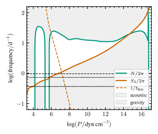
Figure 1: Propagation diagram for the KOI-54 model discussed in the text, plotting the Brunt-Väisälä ($N$) and Lamb ($S_{\ell}$) frequencies as a function of pressure coordinate for $\ell=2$ modes. The hatched regions indicate the acoustic wave ($\sigma>N,S_{\ell}$) and internal gravity wave q($\sigma<N,S_{\ell}$) propagation regions. The sloped dashed line shows the frequency corresponding to the local thermal timescale $t_{\rm thm}$ (equation 19), while the upper (lower) horizontal dashed line corresponds to a frequency $\sigma/\Omega_{\rm orb}=30$ (15).

KOI-54 is a highly-eccentric ($e\approx 0.8$), near face-on binary system comprising a pair of A-type stars. Discovered by Welsh et al. (2011) in Kepler observations, it serves as the archetype of the heartbeat class of periodic variables (Thompson et al., 2012). B12 and Fuller & Lai (2012) each present initial attempts to model the light curve of KOI-54 in terms of contributions from the equilibrium tide, dynamical tides and stellar irradiation. Here we undertake a calculation to reproduce Fig. 6 of B12, which illustrates how a model for the KOI-54 primary responds to forcing by a single partial tidal potential.

Guided by the parameters given in Table 1 of B12, we use release r22.11.1 of the MESA software instrument (Paxton et al., 2011, 2013, 2015, 2018, 2019; Jermyn et al., 2022) to evolve a $2.32\text{\,}\mathrm{M}_{\odot}$ model from the zero-age main sequence (ZAMS) until its photospheric radius has expanded to $2.19\text{\,}\mathrm{R}_{\odot}$. Input files for this and subsequent MESA calculations are available through Zenodo at 10.5281/zenodo.7489814 (catalog 10.5281/zenodo.7489814). The growth of the core is followed using the convective premixing algorithm (Paxton et al., 2019), but rotation is neglected. We avoid any smoothing of the Brunt-Väisälä frequency profile, as this can introduce small but consequential departures from mass conservation. Fundamental parameters for the model are summarized in Table 1, and its propagation diagram is plotted in Fig. 1.

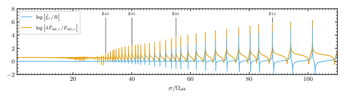
Figure 2: Plot of the radial displacement perturbation $\tilde{\xi}_{{\rm r}}$ and the Lagrangian radial flux perturbation $\delta\tilde{F}_{{\rm rad},r}$ at the surface of the KOI-54 model, as a function of forcing frequency $\sigma$. Selected peaks are labeled by the resonant mode’s classification within the Eckart-Osacki-Scuflaire scheme.

Figure 6 of B12 plots the modulus of $\tilde{\xi}_{{\rm r}}$ and $\delta\tilde{F}_{{\rm rad},r}$ as a function of $\sigma/\Omega_{\rm orb}$, for a single partial potential with $\ell=2$. The choices of $m$ and $k$ are left undetermined because B12 neglect rotation in their figure, and treat $\sigma$ as a free parameter rather than being constrained by equation (E4). They normalize the strength of the partial potential in a manner equivalent to setting $y_{\rm T}=1$ in equation (15). We use gyre_tides to repeat these steps for our KOI-54 model, plotting the results in Fig. 2.

This figure shows qualitative agreement with Fig. 6 of B12. For $\sigma/\Omega_{\rm orb}\gtrsim 30$ the surface perturbations exhibit distinct peaks, corresponding to resonances with the star’s $\ell=2$ free-oscillation modes. Selected peaks are labeled with the resonant mode’s classification within the Eckart-Osaki-Scuflaire scheme (e.g., Unno et al., 1989). For $\sigma/\Omega_{\rm orb}\lesssim 30$ the peaks merge together and dissolve, because the periods of the resonant modes become appreciably shorter than the local thermal timescale

$$t_{\rm thm}(r)\equiv\int_{r}^{R}\frac{4\pi r^{2}\rho Tc_{P}}{L}\operatorname{d}\!{r}$$ (19)

in the outer parts of the main mode-trapping cavity (see Fig. 1), resulting in significant radiative-diffusion damping that broadens and suppresses the resonances. Eventually, for $\sigma/\Omega_{\rm orb}\lesssim 15$ the surface perturbations reach the limits $\tilde{\xi}_{{\rm r}}/R\rightarrow 1$ and $\delta\tilde{F}_{{\rm rad},r}/F_{{\rm rad},r}\rightarrow 4$ corresponding to the $\ell=2$ equilibrium tide (see Section 6.2 of B12 for a discussion of these limits).

On closer inspection, some differences between the two figures are apparent. While the KOI-54 stellar models in B12 and the present work are similar (in particular, sharing the same $M$ and $R$), they are not identical; therefore, the locations and heights of the resonance peaks are not the same in each figure. More significantly, over the range $5\lesssim\sigma/\Omega_{\rm orb}\lesssim 30$ the flux perturbation behaves much more smoothly in Fig. 2 than in Fig. 6 of B12. The reason for this discrepancy is not obvious, but we speculate that it may be linked to differences in the near-surface convection of the models. The propagation diagram for our KOI-54 model (Fig. 1) shows a Heii convection zone at $\log(P/$\mathrm{dyn}\text{\,}{\mathrm{cm}}^{-2}$)\approx 5.5$, but this zone is absent in B12’s model (cf. their Fig. 1).

4.2 Direct Solution versus Mode Decomposition in a KOI-54 Model

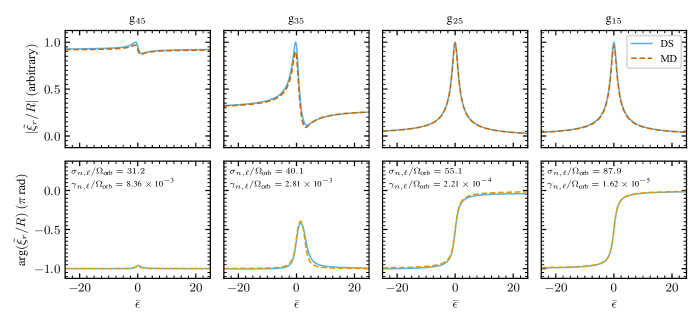
Figure 3: Zoom-in on the four labeled resonance peaks in Fig. 2, plotting the complex amplitude (upper panels; rescaled to have a maximum value of unity) and phase (lower panels) of $\tilde{\xi}_{{\rm r}}/R$ as a function of normalized detuning parameter $\epsilon$ (equation 20). Separate curves are shown for the DS (gyre_tides) and MD approaches.

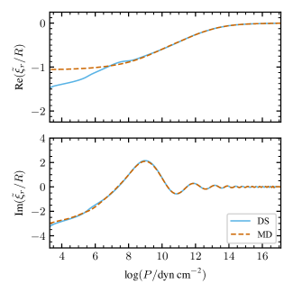
Figure 4: Real (upper panel) and imaginary (lower panel) parts of the wavefunctions associated with the radial displacement perturbation $\tilde{\xi}_{{\rm r}}$ at the peak of the ${\rm g}_{35}$ resonance, plotted as a function of pressure coordinate. The separate curves correspond to the DS (gyre_tides) and MD approaches.

As a validation of the results presented in Fig. 2, we re-calculate the surface perturbations using the MD approach. We follow the formalism laid out in Section 3.2 of B12, although adopting non-adiabatic eigenfrequencies $\sigma_{n,\ell}$ and damping rates $\gamma_{n,\ell}$ provided by gyre to evaluate the Lorentzian factor $\Delta_{n,\ell,m,k}$ (their equation 13; here, $n$ is the mode radial order). To evaluate the overlap integrals $Q_{n,\ell}$ that weight the contribution of each free-oscillation mode in the MD superposition, we use the third expression of equation (9) in B12; we find that the the first expression yields unreliable values when $|n|\gtrsim 20$, because the integrand is highly oscillatory and suffers from significant cancellation.

Figure 3 zooms in on the four labeled resonance peaks from Fig. 2, plotting the complex amplitude and phase of $\tilde{\xi}_{{\rm r}}$ as a function of normalized detuning parameter

$$\bar{\epsilon}\equiv\frac{\sigma-\sigma_{n,\ell}}{|\gamma_{n,\ell}|},$$ (20)

for the two approaches. DS (i.e., gyre_tides) and MD agree at higher forcing frequencies (right-hand panels), but show mismatches toward lower frequencies (left-hand panels).

To delve further into these discrepancies, Fig. 4 plots the $\tilde{\xi}_{{\rm r}}$ wavefunction evaluated at the peak ($\bar{\epsilon}=0$) of the ${\rm g}_{35}$ resonance. The imaginary part of the wavefunction is spatially oscillatory because it is dominated by the dynamical tide, comprising the resonantly forced oscillation mode. The real part is non-oscillatory and corresponds to the equilibrium tide, comprising the superposition of the other, non-resonant $\ell=2$ modes.

The discrepancies in the wavefunction are restricted to the outer parts of the stellar envelope. For $\operatorname{Re}(\tilde{\xi}_{{\rm r}})$, the DS and MD curves begin to diverge at $\log(P/$\mathrm{dyn}\text{\,}{\mathrm{cm}}^{-2}$)\approx 8$ (corresponding to $r/R\gtrsim 0.96$), while for $\operatorname{Im}(\tilde{\xi}_{{\rm r}})$ the divergence begins further out at $\log(P/$\mathrm{dyn}\text{\,}{\mathrm{cm}}^{-2}$)\approx 6$ ($r/R\approx 0.99$). We hypothesize that these divergences arise because $\sigma\ll 2\pi/t_{\rm thm}$ in these superficial layers, leading to significant non-adiabaticity that MD is unable to correctly reproduce (see Section 6.2 of B12; also, Section 6 of Fuller, 2017).

4.3 Circularization in a B-star Model

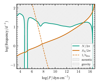
Figure 5: Propagation diagram for the B-star model introduced in the text (cf. Fig. 1). The dip in the Brunt-Väisälä frequency around $\log(P/$\mathrm{dyn}\text{\,}{\mathrm{cm}}^{-2}$)\approx 7.5$ is caused by the iron opacity bump responsible for the overstability of the ${\rm g}_{9}-{\rm g}_{17}$ modes.

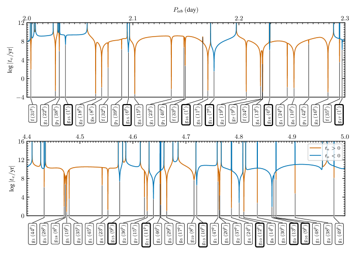
Figure 6: The circularization timescale $t_{e}$ plotted as a function of orbital period $P_{\rm orb}$, for the binary system with the B-star primary. Resonances are labeled beneath with the mode classification, and in parentheses the harmonic index $k$ and the sense of propagation in the co-rotating frame (p=prograde, r=retrograde). If the resonance is with an overstable mode, then the label border is bolded.

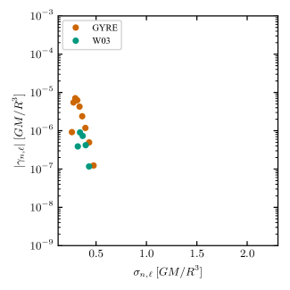
Figure 7: Damping rates $\gamma_{n,\ell}$ plotted against eigenfrequencies $\sigma_{n,\ell}$ for ${\rm g}_{1}$–${\rm g}_{20}$ modes of the B-star model, as calculated using gyre and as tabulated by W03. Open symbols indicate stable ($\gamma_{n,\ell}>0$) modes, and filled symbols overstable ($\gamma_{n,\ell}<0$) modes.

Willems et al. (2003, hereafter W03) explore the secular orbital changes due to tides in a binary system comprising a $5\text{\,}\mathrm{M}_{\odot}$ B-star primary and a $1.4\text{\,}\mathrm{M}_{\odot}$ secondary on an $e=0.5$ orbit. They adopt the MD approach, but include only a single term at a time in the modal superposition. The calculations illustrated in Fig. 3 of W03 are used by Valsecchi et al. (2013) to benchmark their CAFein code, motivating us to do likewise here with gyre_tides.

We use MESA as before to evolve a $5\text{\,}\mathrm{M}_{\odot}$ model from the ZAMS until its photospheric radius has grown to match the $2.80\text{\,}\mathrm{R}_{\odot}$ of W03’s model. Fundamental parameters for this model are summarized in Table 1, and its propagation diagram is plotted in Fig. 5. Then, we apply gyre_tides to evaluate the star’s response to the dominant contributions in the tidal potential (8), comprising the $\ell=2$ terms with $|m|=2$ and $mk>0$. We further restrict the summation over $k$ to terms with a magnitude at least $10^{-12}$ times that of the largest term. As in W03, we assume the stellar angular rotation frequency is equal to the periastron angular velocity of the secondary,

$$\Omega_{\rm peri}=\Omega_{\rm orb}\,\sqrt{\frac{(1+e)}{(1-e)^{3}}}.$$ (21)

Based on this configuration, Fig. 6 plots the circularization timescale

$$t_{e}\equiv-\left[\frac{1}{e}\left(\frac{\operatorname{d}\!{e}}{\operatorname{d}\!{t}}\right)\right]^{-1}_{\rm sec}$$ (22)

as a function of orbital period $P_{\rm orb}\equiv 2\pi/\Omega_{\rm orb}$ over a pair of intervals. The secular rate-of-change of eccentricity is evaluated via

$$\left(\frac{\operatorname{d}\!{e}}{\operatorname{d}\!{t}}\right)_{\rm sec}=4\,\Omega_{\rm orb}\,q\sum_{\ell,m,k\geq 0}\left(\frac{R}{a}\right)^{\ell+3}\,\left(\frac{r_{\rm s}}{R}\right)^{\ell+1}\\ \mbox{}\times\kappa_{\ell,m,k}\,\operatorname{Im}(\bar{F}_{\ell,m,k})\,\bar{G}^{(3)}_{\ell,m,k};$$ (23)

this comes from equation (55) of Willems et al. (2010), with $F_{\ell,m,k}$ replaced by $\bar{F}_{\ell,m,k}\equiv F_{\ell,m,-k}$ and $G^{(3)}_{\ell,m,k}$ by $\bar{G}^{(3)}_{\ell,m,k}\equiv G^{(3)}_{\ell,m,-k}$ to account for the differing sign convention in the assumed time dependence of partial tides (see equation 13). Note that the summation is now restricted to $k\geq 0$.

The $|t_{e}|$ data plotted in the figure vary smoothly with $P_{\rm orb}$ between a series of sharp extrema. The maxima (more correctly, singularities) arise when $(\operatorname{d}\!{e}/\operatorname{d}\!{t})_{\rm sec}$ passes through zero. The minima arise from resonances with the star’s $\ell=2$ free-oscillation modes, similar to the peaks seen in Fig. 2. However, a key difference here is that the star is being forced with a superposition (8) of partial tidal potentials, rather than a single one as before. The criterion for resonance $\sigma_{m,k}\approx\sigma_{n,\ell}$ can be satisfied for many different values of $k$, leading to multiple resonances with the same mode. This can be seen in the figure; for instance, the upper panel shows resonances between the $f$ mode and the partial tidal potentials with $k=31,\ldots,35$.

In the vicinity of some of the resonances shown in the figure, $t_{e}<0$ (blue) indicates that the tide acts to increase the eccentricity of the orbit, driving it further away from circular. This behavior is an instance of the ‘inverse tides’ phenomenon discussed by Fuller (2021), and occurs when the summation in equation (23) is dominated by a single, positive term. There are four distinct configurations that lead to this outcome:

1. $\bar{G}^{(3)}_{\ell,m,k}>0$ and $\operatorname{Im}(\bar{F}_{\ell,m,k})>0$, the latter because

   1. the resonant mode is prograde in the co-rotating frame ($\sigma_{n,\ell}/m>0$) and stable ($\gamma_{n,\ell}>0$); or

   2. the resonant mode is retrograde in the co-rotating frame ($\sigma_{n,\ell}/m<0$) and overstable ($\gamma_{n,\ell}<0$).

2. $\bar{G}^{(3)}_{\ell,m,k}<0$ and $\operatorname{Im}(\bar{F}_{\ell,m,k})<0$, the latter because

   1. the resonant mode is prograde in the co-rotating frame ($\sigma_{n,\ell}/m>0$) and overstable ($\gamma_{n,\ell}<0$); or

   2. the resonant mode is retrograde in the co-rotating frame ($\sigma_{n,\ell}/m<0$) and stable ($\gamma_{n,\ell}>0$).

All of the $t_{e}<0$ resonances seen in Fig. 6 are instances of cases (I.b) or (II.a), and therefore involve overstable modes. The overstability is caused by the iron-bump opacity mechanism responsible for the slowly pulsating B (SPB) stars (e.g., Gautschy & Saio, 1993; Dziembowski et al., 1993); in the B-star model considered here, which falls well inside the SPB instability strip (e.g., Pamyatnykh, 1999; Paxton et al., 2015), this mechanism excites the $\ell=2$ ${\rm g}_{9}$–${\rm g}_{17}$ modes.

Comparing Fig. 6 against Fig. 3 of W03 reveals some important differences. The latter shows numerous gaps and discontinuities in $t_{e}$, that appear to arise because W03 only allow a given mode to contribute toward the MD superposition when its detuning parameter (equation 20) satisfies $0.1\,\varepsilon_{\rm T}\leq|\bar{\epsilon}\gamma_{n,\ell}/\sigma_{n,\ell}|\leq 10\,\varepsilon_{\rm T}$. The lower bound on $\bar{\epsilon}$ means that the central parts of each resonance are omitted, and so Fig. 3 of W03 does not fully reveal how small $t_{e}$ can become when close to a resonance.

At the short-period limit of the range shown in the figures, there is also disagreement between the typical magnitude of $t_{e}$ between the resonances; Fig. 6 shows an inter-resonance $|t_{e}|\approx${10}^{9}\text{\,}\mathrm{yr}$$ , whereas for W03 it is 2–4 orders of magnitude shorter. This is likely a consequence of W03 over-estimating the damping for the ${\rm g}_{1}$–${\rm g}_{4}$ modes, which dominate the tidal response at short orbital periods. Figure 7 plots eigenfrequencies $\sigma_{n,\ell}$ and damping rates $\gamma_{n,\ell}$ for the ${\rm g}_{1}$–${\rm g}_{20}$ modes, as calculated using gyre and as obtained from Table 1 of W03. The data for the ${\rm g}_{5}$–${\rm g}_{16}$ modes are in reasonable agreement, especially given that the underlying stellar models do not have the exact same internal structure. However, the W03 damping rates for the ${\rm g}_{1}$–${\rm g}_{4}$ modes are four-to-five orders of magnitude larger than the gyre ones.

4.4 Pseudo-Synchronization in a KOI-54 Model

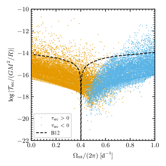
Figure 8: Secular torque $\mathcal{T}_{\rm sec}$ plotted against stellar angular rotation frequency $\Omega_{\rm rot}$ for the KOI-54 primary model. The dashed line shows the equilibrium-tide torque extracted from Fig. 4 of B12.

B12 explore how tides can modify the rotation of the primary star in the KOI-54 system, by evaluating the secular tidal torque $\mathcal{T}_{\rm sec}$ on the primary star as a function of the star’s rotation rate. Using an MD approach (see their Appendix C), they consider contributions toward the torque from the $\ell=2$ partial tidal potentials. Their Fig. 4 shows a smoothly varying $\mathcal{T}_{\rm sec}$ punctuated by many narrow peaks due to modal resonances. The smooth part corresponds to the torque from the equilibrium tide, and passes through zero at the pseudo-synchronous angular frequency

$$\Omega_{\rm ps}\equiv\Omega_{\rm orb}\frac{1+(15/2)e^{2}+(45/8)e^{4}+(5/16)e^{6}}{[1+3e^{2}+(3/8)e^{4}](1-e)^{3/2}}$$ (24)

first derived by Hut (1981) in his theory of tides in the weak friction limit. For the orbital parameters of KOI-54, the pseudo-synchronous frequency is $\Omega_{\rm ps}/(2\pi)=$0.395\text{\,}{\mathrm{d}}^{-1}$$.

To repeat this calculation, we use gyre_tides to evaluate the response of the KOI-54 model (Section 4.1) to the $\ell=2$ terms in the tidal potential (Equation 8) for $25,000$ rotation frequencies in the interval $$0\text{\,}{\mathrm{d}}^{-1}$\leq\Omega_{\rm rot}/(2\pi)\leq$1\text{\,}{\mathrm{d}}^{-1}$$. As in the preceding section, we restrict the summation over $k$ to terms with a magnitude at least $10^{-12}$ times that of the largest term. Then, we evaluate the tidal torque via

$$\mathcal{T}_{\rm sec}=4\Omega_{\rm orb}\sqrt{\frac{GM^{3}q^{2}}{1+q}}\,q\,a^{1/2}\sum_{\ell,m,k\geq 0}\left(\frac{R}{a}\right)^{\ell+3}\,\left(\frac{r_{\rm s}}{R}\right)^{\ell+1}\\ \times\kappa_{\ell,m,k}\,\operatorname{Im}(\bar{F}_{\ell,m,k})\,\bar{G}^{(4)}_{\ell,m,k};$$ (25)

this comes from equation (63) of Willems et al. (2010), with $G^{(4)}_{\ell,m,k}$ replaced by $\bar{G}^{(4)}_{\ell,m,k}\equiv G^{(4)}_{\ell,m,-k}$.

Fig. 8 plots $\mathcal{T}_{\rm sec}$ as a function of $\Omega_{\rm rot}$, using discrete points rather than a continuous line because we are significantly undersampling the dense forest of resonances. Also plotted for comparison is the smooth (equilibrium tide) part of the torque extracted from Fig. 4 of B12. Clearly, there are some significant differences between the two figures. Ours shows a torque that’s generally positive torque at small rotation frequencies, and negative at high frequencies; however, the switch-over point is not nearly as sharply defined as in B12, and occurs at a frequency $\Omega_{\rm rot}/(2\pi)\approx$0.5\text{\,}{\mathrm{d}}^{-1}$$ around 25% higher than $\Omega_{\rm ps}$. Moreover, on either side of the switch-over, the lower envelope of our torque values is around two orders of magnitude smaller than the B12 curve.

Exploratory calculations indicate that these differences are not a result of inaccurate overlap integrals (as was the case in Section 4.2), but rather due to a genuine incompatibility between the DS and MD approaches. While a detailed investigation of this problem is beyond the scope of the present paper, we believe the fault lies with MD’s over-estimation of radiative dissipation for the equilibrium tide. If this hypothesis is correct, an immediate corollary is that pseudo-synchronization as envisaged by Hut (1981) does not operate for stars in which radiative dissipation dominates the tidal damping.

5 Summary and Discussion

To briefly summarize the preceding sections: we establish the theoretical foundations for our tides treatment (Section 2), describe modifications to GYRE to implement tides (Section 3), and then apply the new gyre_tides executable to selected problems (Section 4). These example calculations uncover disagreements between the DS and MS approaches, arising for a variety of reasons — from numerical inaccuracies in overlap integrals (Section 4.2), through to what appears to be an incompatibility between the approaches. We look forward to future opportunities to investigate these disagreements.

We also plan a number of enhancements to gyre_tides that will extend its capabilities. Key milestones include adding the ability to model systems with spin-orbit misalignments (e.g., following the formalism described by Fuller, 2017); the incorporation of additional damping mechanisms beyond radiative diffusion (for instance, turbulent viscosity within convection zones; see Willems et al., 2010); and treating the effects of the Coriolis force, which was neglected in deriving the linearized equations (Appendix D). Partial treatment of the Coriolis force is already included in the main gyre executable, via the traditional approximation of rotation (TAR; see, e.g., Bildsten et al., 1996; Lee & Saio, 1997; Townsend, 2003). However, in its current form this implementation cannot be used in gyre_tides, because the angular operator appearing in the linearized continuity equation within the TAR (see equation 6 of Bildsten et al., 1996) does not commute with the angular part of the Laplacian operator appearing in the linearized Poisson equation (D3).

GYRE is not the first software package that adopts the DS approach to model stellar tides; Pfahl et al. (2008) and Valsecchi et al. (2013) describe functionally similar codes. Although the former authors’ code has never been made publicly available, the latters’ CAFein code is accessible on GitHub. After fixing a number of bugs in CAFein (for instance, relating to misinterpreting cell-centered quantities in MESA models as face-centered), we have undertaken exploratory calculations comparing it against gyre_tides, and find the two codes are in general agreement. Given that CAFein is unmaintained, we decided that more-detailed comparison would not be a worthwhile exercise.

It is our hope that gyre_tides will provide a standardized and well-supported community tool for simulating tides of spherical stars within the linear limit. Specific areas where we anticipate productive applications include modeling the many heartbeat systems discovered by Kepler (e.g., Thompson et al., 2012), TESS (e.g., Kołaczek-Szymański et al., 2021) and OGLE (Wrona et al., 2022); investigating why most of these systems rotate faster than the pseudo-synchronous rate (Zimmerman et al., 2017); and exploring orbital and rotational evolution in more-general star-star and star-planet systems. These latter activities will initially be restricted to cases where radiative diffusion dominates the tidal damping (e.g., the $\gamma$ Doradus stars considered by Li et al., 2020a); but with the planned addition of other damping mechanisms, they can be extended more broadly.

Appendix A Expansion Coefficients

The expansion coefficients appearing in equation. (9) are given by

$$\bar{c}_{\ell,m,k}=\frac{4\pi}{2\ell+1}\,\left(\frac{R}{a}\right)^{\ell-2}\,{Y^{m}_{\ell}}^{*}(\pi/2,0)\,X^{-(\ell+1),-m}_{-k},$$ (A1)

where $Y^{m}_{\ell}$ is a spherical harmonic (Appendix B) and $X^{-(\ell+1),-m}_{-k}$ is a Hansen coefficient (Appendix C). They are related to the $c_{\ell,m,k}$ coefficients defined by Willems et al. (2010) via

$$\bar{c}_{\ell,m,k}=(-1)^{(|m|-m)/2}\,\sqrt{\frac{4\pi}{2\ell+1}\frac{(l+|m|)!}{(l-|m|)!}}\,c_{\ell,m,-k}.$$ (A2)

Appendix B Spherical Harmonics

There are a number of alternate definitions of the spherical harmonics, differing in normalization and phase conventions. We follow Arfken et al. (2013) and adopt

$$Y^{m}_{\ell}(\vartheta,\varphi)=\sqrt{\frac{2\ell+1}{4\pi}\frac{(\ell-m)!}{(\ell+m)!}}P^{m}_{\ell}(\cos\vartheta)\operatorname{e}^{im\varphi}.$$ (B1)

The associated Legendre functions are in turn defined by the Rodrigues formula

$$P^{m}_{\ell}(x)=\frac{(-1)^{m}}{2^{\ell}\ell!}\left(1-x^{2}\right)^{m/2}\frac{\operatorname{d}^{\ell+m}\!\!{}}{\operatorname{d}\!{x}^{\ell+m}}\left(x^{2}-1\right)^{\ell}$$ (B2)

[the extra $(-1)^{m}$ factor is the Condon-Shortley phase term]. With these definitions, the spherical harmonics obey the orthonormality condition

$$\int_{0}^{2\pi}\int_{0}^{\pi}Y^{m}_{\ell}\,Y^{m^{\prime}*}_{\ell^{\prime}}\,\sin\vartheta\,\operatorname{d}\!{\vartheta}\operatorname{d}\!{\varphi}=\delta_{\ell,\ell^{\prime}}\delta_{m,m^{\prime}},$$ (B3)

and moreover the relation

$${Y^{m}_{\ell}}^{*}=(-1)^{m}Y^{-m}_{\ell}.$$ (B4)

Appendix C Hansen Coefficients

The Hansen coefficients are defined implicitly by the equation

$$\left(\frac{r_{2}}{a}\right)^{n}\operatorname{e}^{\mathrm{i}m\upsilon}=\sum_{k=-\infty}^{\infty}X^{n,m}_{k}\operatorname{e}^{\mathrm{i}k\mathcal{M}}$$ (C1)

(e.g., Hughes, 1981). They can be evaluated via

$$X^{n,m}_{k}=\frac{(1-e^{2})^{n}}{2\pi}\int_{-\pi}^{\pi}(1+e\cos\mathcal{M})^{-n}\cos(m\upsilon-k\mathcal{M})\,\operatorname{d}\!{\mathcal{M}};$$ (C2)

however, an equivalent form due to Smeyers et al. (1991),

$$X^{n,m}_{k}=\frac{(1-e^{2})^{n+3/2}}{2\pi}\int_{-\pi}^{\pi}(1+e\cos\mathcal{M})^{-n-2}\cos(m\upsilon-k\mathcal{M})\,\operatorname{d}\!{\upsilon},$$ (C3)

is more convenient because it does not require Kepler’s equation (2) be solved for $\mathcal{E}$. The integrand is periodic with respect to $\upsilon$, and so the exponential convergence of the trapezoidal quadrature rule (Trefethen & Weideman, 2014) is ideal for evaluating this integral.

Appendix D Linearized Equations

We introduce the tidal potential $\Phi_{{\rm T}}$ (equation 8) into the fluid equations governing the primary star as a small ($\varepsilon_{\rm T}\ll 1$) perturbation about the equilibrium state. We assume this equilibrium state is spherically symmetric and static; while we allow for uniform rotation about the $z$-axis with angular velocity $\Omega_{\rm rot}$, we neglect the inertial (Coriolis and centrifugal) forces arising from this rotation. Discarding terms of second- or higher-order in $\varepsilon_{\rm T}$ from the perturbed structure equations, and subtracting away the equilibrium state, yields linearized versions of the fluid equations. These comprise the mass equation

$$\left(\frac{\partial{}}{\partial{t}}+\Omega_{\rm rot}\frac{\partial{}}{\partial{\varphi}}\right)\rho^{\prime}+\nabla\cdot(\rho\mathbf{v}^{\prime})=0;$$ (D1)

the momentum equation

$$\sum_{i=\{r,\vartheta,\varphi\}}\left[\left(\frac{\partial{}}{\partial{t}}+\Omega_{\rm rot}\frac{\partial{}}{\partial{\varphi}}\right)v^{\prime}_{i}\right]\mathbf{e}_{i}=-\frac{1}{\rho}\nabla P^{\prime}+\frac{\rho^{\prime}}{\rho^{2}}\frac{\operatorname{d}\!{P}}{\operatorname{d}\!{r}}-\nabla\Psi^{\prime},$$ (D2)

where $\Psi^{\prime}\equiv\Phi^{\prime}+\Phi_{{\rm T}}$; Poisson’s equation

$$\nabla^{2}\Psi^{\prime}=4\pi G\rho^{\prime};$$ (D3)

the heat equation

$$T\left(\frac{\partial{}}{\partial{t}}+\Omega_{\rm rot}\frac{\partial{}}{\partial{\varphi}}\right)\delta S=\delta\epsilon-\delta\left[\frac{1}{\rho}\nabla\cdot(\mathbf{F}_{\rm rad}+\mathbf{F}_{\rm con})\right];$$ (D4)

and the radiative diffusion equation

$$\delta\mathbf{F}_{\rm rad}=\left(4\frac{\delta T}{T}-\frac{\delta\rho}{\rho}-\frac{\delta\kappa}{\kappa}\right)\mathbf{F}_{\rm rad}+\frac{\delta\left(\nabla\ln T\right)}{\operatorname{d}\!{\ln T}/\operatorname{d}\!{r}}F_{{\rm rad},r}.$$ (D5)

In these equations, $\mathbf{v}$ is the fluid velocity; $P$, $T$, $\rho$, and $S$ are the pressure, density, temperature, and specific entropy, respectively; $\mathbf{F}_{\rm rad}$ and $\mathbf{F}_{\rm con}$ are the radiative and convective flux vectors, with $F_{{\rm rad},r}$ the radial component of the former; $\kappa$ is the opacity and $\epsilon$ the specific nuclear energy generation rate; and $\Phi$ is the self-gravitational potential. A prime (^′) suffix on a quantity indicates the Eulerian (fixed position) perturbation, while a $\delta$ prefix indicates the Lagrangian (fixed mass element) perturbation; the absence of either modifier signifies the equilibrium state. To first order, Eulerian and Lagrangian perturbations to a quantity $f$ are linked through

$$\delta f=f^{\prime}+(\boldsymbol{\xi}\cdot\nabla)f,$$ (D6)

where the displacement perturbation vector $\boldsymbol{\xi}$ is related to the velocity perturbation $\mathbf{v}^{\prime}$ via

$$\mathbf{v}^{\prime}=\sum_{i=\{r,\vartheta,\varphi\}}\left[\left(\frac{\partial{}}{\partial{t}}+\Omega_{\rm rot}\frac{\partial{}}{\partial{\varphi}}\right)\xi_{i}\right]\mathbf{e}_{i}.$$ (D7)

The system of differential equations (D1–D5) is augmented by a convective freezing prescription

$$\delta\left(\frac{1}{\rho}\nabla\cdot\mathbf{F}_{\rm con}\right)=0$$ (D8)

(this corresponds to approach 1 in the classification scheme by Pesnell, 1990), together with the linearized thermodynamic relations

$$\frac{\delta\rho}{\rho}=\frac{1}{\Gamma_{1}}\frac{\delta P}{P}-\upsilon_{T}\frac{\delta S}{c_{P}},\qquad\frac{\delta T}{T}=\nabla_{\rm ad}\frac{\delta P}{P}+\frac{\delta S}{c_{P}},$$ (D9)

and the linearized microphysics equations

$$\frac{\delta\kappa}{\kappa}=\kappa_{\rm ad}\frac{\delta P}{P}+\kappa_{S}\frac{\delta S}{c_{P}},\qquad\frac{\delta\epsilon}{\epsilon}=\epsilon_{\rm ad}\frac{\delta P}{P}+\epsilon_{S}\frac{\delta S}{c_{P}}.$$ (D10)

Here,

$$\begin{gathered}\Gamma_{1}\equiv\left(\frac{\partial{\ln P}}{\partial{\ln\rho}}\right)_{S},\qquad\nabla_{\rm ad}\equiv\left(\frac{\partial{\ln T}}{\partial{\ln P}}\right)_{S},\qquad\upsilon_{T}\equiv-\left(\frac{\partial{\ln\rho}}{\partial{\ln T}}\right)_{P},\qquad c_{P}\equiv\left(\frac{\partial{S}}{\partial{\ln T}}\right)_{P}\\ \kappa_{\rm ad}\equiv\left(\frac{\partial{\ln\kappa}}{\partial{\ln P}}\right)_{S},\qquad\kappa_{S}\equiv c_{P}\left(\frac{\partial{\ln\kappa}}{\partial{S}}\right)_{P},\qquad\epsilon_{\rm ad}\equiv\left(\frac{\partial{\ln\epsilon}}{\partial{\ln P}}\right)_{S},\qquad\epsilon_{S}\equiv c_{P}\left(\frac{\partial{\ln\epsilon}}{\partial{S}}\right)_{P}.\end{gathered}$$ (D11)

The system of equations is closed by applying boundary conditions at the center and surface of the primary star. At the center we require that perturbations remain regular. At the surface, the boundary conditions are composed of the vacuum condition

$$\delta P=0,$$ (D12)

the linearized Stefan-Boltzmann law

$$\frac{\delta L_{\rm R}}{L_{\rm R}}=2\frac{\xi_{\rm r}}{R}+4\frac{\delta T}{T},$$ (D13)

where $L_{\rm R}\equiv 4\pi r^{2}F_{{\rm rad},r}$ is the radiative luminosity, and the requirement that $\delta\Psi$ and its gradient are continuous across the surface.

Appendix E Tidal Equations

The tidal equations govern the radial functions appearing in the solution forms (11,12). To obtain these equations for a given combination of indices $\{\ell^{\prime},m^{\prime},k^{\prime}\}$, we substitute these solution forms into the linearized equations (Appendix D), multiply by a weighting factor $H_{\ell^{\prime},m^{\prime},k^{\prime}}^{*}$, and then integrate over $4\pi$ steradians and one orbital period. Following these steps, the mass equation (D1) becomes

$$\frac{\delta\tilde{\rho}}{\rho}+\frac{1}{r^{2}}\frac{\operatorname{d}\!{}}{\operatorname{d}\!{r}}\left(r^{2}\tilde{\xi}_{{\rm r}}\right)-\frac{\ell(\ell+1)}{r}\tilde{\xi}_{{\rm h}}=0$$ (E1)

(for notational compactness and clarity, here and subsequently we omit the $\ell,m,k$ subscripts on dependent variables such as $\tilde{\rho}_{\ell,m,k}$ and $\tilde{\xi}_{{\rm r};\ell,m,k}$). The radial and horizontal components of the momentum equation (D2) become

$$\sigma_{m,k}^{2}\,\tilde{\xi}_{{\rm r}} =\frac{1}{\rho}\frac{\operatorname{d}\!{\tilde{P}^{\prime}}}{\operatorname{d}\!{r}}-\frac{\tilde{\rho}^{\prime}}{\rho^{2}}\frac{\operatorname{d}\!{P}}{\operatorname{d}\!{r}}+\frac{\operatorname{d}\!{\tilde{\Psi}^{\prime}}}{\operatorname{d}\!{r}},$$ (E2)

$$\sigma_{m,k}^{2}\,\tilde{\xi}_{{\rm h}} =\frac{1}{r}\left(\frac{\tilde{P}^{\prime}}{\rho}+\tilde{\Psi}^{\prime}\right),$$ (E3)

respectively, where

$$\sigma_{m,k}\equiv k\Omega_{\rm orb}-m\Omega_{\rm rot}$$ (E4)

represents the tidal forcing frequency measured in a frame rotating with the primary star. Poisson’s equation (D3) becomes

$$\frac{1}{r^{2}}\frac{\operatorname{d}\!{}}{\operatorname{d}\!{r}}\left(r^{2}\frac{\operatorname{d}\!{\tilde{\Psi}^{\prime}}}{\operatorname{d}\!{r}}\right)-\frac{\ell(\ell+1)}{r^{2}}\tilde{\Psi}^{\prime}=4\pi G\tilde{\rho}^{\prime},$$ (E5)

while the heat equation (D4), expressed in terms of $L_{\rm R}$ and its perturbation, becomes

$$-\mathrm{i}\sigma_{m,k}\,T\delta\tilde{S}=\delta\tilde{\epsilon}-\frac{1}{4\pi r^{2}\rho}\frac{\operatorname{d}\!{\delta\tilde{L}_{{\rm R}}}}{\operatorname{d}\!{r}}+\frac{\ell(\ell+1)}{\operatorname{d}\!{\ln T}/\operatorname{d}\!{\ln r}}\frac{L_{\rm R}}{4\pi r^{3}\rho}\frac{\tilde{T}^{\prime}}{T}+\ell(\ell+1)\frac{\tilde{\xi}_{{\rm h}}}{4\pi r^{3}\rho}\frac{\operatorname{d}\!{L_{\rm R}}}{\operatorname{d}\!{r}}.$$ (E6)

(equation D8 has been used to eliminate the convective terms from this equation.) The radiative diffusion equation (D5) becomes

$$\frac{\delta\tilde{L}_{{\rm R}}}{L_{\rm R}}=-\frac{\delta\tilde{\kappa}}{\kappa}+4\frac{\tilde{\xi}_{{\rm r}}}{r}-\ell(\ell+1)\frac{\tilde{\xi}_{{\rm h}}}{r}+4\frac{\delta\tilde{T}}{T}+\frac{1}{\operatorname{d}\!{\ln T}/\operatorname{d}\!{\ln r}}\frac{\operatorname{d}\!{(\delta\tilde{T}/T)}}{\operatorname{d}\!{r}}.$$ (E7)

The thermodynamic relations (D9) become

$$\frac{\delta\tilde{\rho}}{\rho}=\frac{1}{\Gamma_{1}}\frac{\delta\tilde{P}}{P}-\upsilon_{T}\frac{\delta\tilde{S}}{c_{P}},\qquad\frac{\delta\tilde{T}}{T}=\nabla_{\rm ad}\frac{\delta\tilde{P}}{P}+\frac{\delta\tilde{S}}{c_{P}},$$ (E8)

and the microphysics relations (D10) become

$$\frac{\delta\tilde{\kappa}}{\kappa}=\kappa_{\rm ad}\frac{\delta\tilde{P}}{P}+\kappa_{S}\frac{\delta\tilde{S}}{c_{P}},\qquad\frac{\delta\tilde{\epsilon}}{\epsilon}=\epsilon_{\rm ad}\frac{\delta\tilde{P}}{P}+\epsilon_{S}\frac{\delta\tilde{S}}{c_{P}}.$$ (E9)

The inner boundary conditions are

$$\tilde{\xi}_{{\rm r}}-\ell\,\tilde{\xi}_{{\rm h}}=0,\qquad\frac{\operatorname{d}\!{\tilde{\Psi}^{\prime}}}{\operatorname{d}\!{r}}-\ell\frac{\tilde{\Psi}^{\prime}}{r}=0,\qquad\delta\tilde{S}=0$$ (E10)

evaluated at the center of the star $r=0$. Finally, the outer boundary conditions are

$$\delta\tilde{P}=0,\qquad\frac{\delta\tilde{L}_{{\rm R}}}{L_{\rm R}}=2\frac{\tilde{\xi}_{{\rm r}}}{R}+4\frac{\delta\tilde{T}}{T},\qquad\frac{\operatorname{d}\!{\tilde{\Psi}^{\prime}}}{\operatorname{d}\!{r}}+\frac{\ell+1}{r}\tilde{\Psi}^{\prime}+4\pi G\rho\,\tilde{\xi}_{{\rm r}}=\frac{2\ell+1}{r}\tilde{\Phi}_{{\rm T};\ell,m,k}$$ (E11)

evaluated at the surface $r=r_{\rm s}$, where we introduce

$$\tilde{\Phi}_{{\rm T};\ell,m,k}\equiv-\varepsilon_{\rm T}\frac{GM}{R}\bar{c}_{\ell,m,k}\left(\frac{r}{R}\right)^{\ell}$$ (E12)

as the radial part of the partial tidal potential (9).

References

- Arfken et al. (2013) Arfken, G. B., Weber, H. J., & Harris, F. E. 2013, Mathematical Methods for Physicists, 7th edn. (Oxford, UK: Academic Press)
- Arras et al. (2003) Arras, P., Flanagan, E. E., Morsink, S. M., et al. 2003, ApJ, 591, 1129, doi: 10.1086/374657
- Astropy Collaboration et al. (2013) Astropy Collaboration, Robitaille, T. P., Tollerud, E. J., et al. 2013, A&A, 558, A33
- Astropy Collaboration et al. (2018) Astropy Collaboration, Price-Whelan, A. M., Sipőcz, B. M., et al. 2018, AJ, 156, 123
- Astropy Collaboration et al. (2022) Astropy Collaboration, Price-Whelan, A. M., Lim, P. L., et al. 2022, ApJ, 935, 167
- Bildsten et al. (1996) Bildsten, L., Ushomirsky, G., & Cutler, C. 1996, ApJ, 460, 827
- Burkart et al. (2012) Burkart, J., Quataert, E., Arras, P., & Weinberg, N. N. 2012, MNRAS, 421, 983
- Chidester et al. (2021) Chidester, M. T., Timmes, F. X., Schwab, J., et al. 2021, ApJ, 910, 24
- Dziembowski et al. (1993) Dziembowski, W. A., Moskalik, P., & Pamyatnykh, A. A. 1993, MNRAS, 265, 588
- Fuller (2017) Fuller, J. 2017, MNRAS, 472, 1538
- Fuller (2021) —. 2021, MNRAS, 501, 483
- Fuller & Lai (2012) Fuller, J., & Lai, D. 2012, MNRAS, 420, 3126
- Gautschy & Saio (1993) Gautschy, A., & Saio, H. 1993, MNRAS, 262, 213
- Goldberg et al. (2020) Goldberg, J. A., Bildsten, L., & Paxton, B. 2020, ApJ, 891, 15
- Goldstein & Townsend (2020) Goldstein, J., & Townsend, R. H. D. 2020, ApJ, 899, 116
- Hughes (1981) Hughes, S. 1981, Celestial Mechanics, 25, 101
- Hunter (2007) Hunter, J. D. 2007, Computing in Science & Engineering, 9, 90
- Hut (1981) Hut, P. 1981, A&A, 99, 126
- Jermyn et al. (2022) Jermyn, A. S., Bauer, E. B., Schwab, J., et al. 2022, arXiv e-prints, arXiv:2208.03651
- Kippenhahn et al. (2013) Kippenhahn, R., Weigert, A., & Weiss, A. 2013, Stellar Structure and Evolution, 2nd edn. (Springer-Verlag, Berlin)
- Kołaczek-Szymański et al. (2021) Kołaczek-Szymański, P. A., Pigulski, A., Michalska, G., Moździerski, D., & Różański, T. 2021, A&A, 647, A12
- Kumar et al. (1995) Kumar, P., Ao, C. O., & Quataert, E. J. 1995, ApJ, 449, 294
- Lai (1997) Lai, D. 1997, ApJ, 490, 847
- Lee & Saio (1997) Lee, U., & Saio, H. 1997, ApJ, 491, 839
- Li et al. (2020a) Li, G., Guo, Z., Fuller, J., et al. 2020a, MNRAS, 497, 4363
- Li et al. (2020b) Li, T., Bedding, T. R., Christensen-Dalsgaard, J., et al. 2020b, MNRAS, 495, 3431
- Li et al. (2022) Li, T., Li, Y., Bi, S., et al. 2022, ApJ, 927, 167
- Mankovich et al. (2019) Mankovich, C., Marley, M. S., Fortney, J. J., & Movshovitz, N. 2019, ApJ, 871, 1
- Michielsen et al. (2021) Michielsen, M., Aerts, C., & Bowman, D. M. 2021, A&A, 650, A175
- Murphy et al. (2022) Murphy, S. J., Bedding, T. R., White, T. R., et al. 2022, MNRAS, 511, 5718
- Nsamba et al. (2021) Nsamba, B., Moedas, N., Campante, T. L., et al. 2021, MNRAS, 500, 54
- Pamyatnykh (1999) Pamyatnykh, A. A. 1999, Acta Astron., 49, 119
- Paxton et al. (2011) Paxton, B., Bildsten, L., Dotter, A., et al. 2011, ApJS, 192, 3
- Paxton et al. (2013) Paxton, B., Cantiello, M., Arras, P., et al. 2013, ApJS, 208, 4
- Paxton et al. (2015) Paxton, B., Marchant, P., Schwab, J., et al. 2015, ApJS, 220, 15
- Paxton et al. (2018) Paxton, B., Schwab, J., Bauer, E. B., et al. 2018, ApJS, 234, 34
- Paxton et al. (2019) Paxton, B., Smolec, R., Schwab, J., et al. 2019, ApJS, 243, 10
- Pesnell (1990) Pesnell, W. D. 1990, ApJ, 363, 227
- Pfahl et al. (2008) Pfahl, E., Arras, P., & Paxton, B. 2008, ApJ, 679, 783
- Polfliet & Smeyers (1990) Polfliet, R., & Smeyers, P. 1990, A&A, 237, 110
- Rindler-Daller et al. (2021) Rindler-Daller, T., Freese, K., Townsend, R. H. D., & Visinelli, L. 2021, MNRAS, 503, 3677
- Savonije & Papaloizou (1983) Savonije, G. J., & Papaloizou, J. C. B. 1983, MNRAS, 203, 581
- Savonije & Papaloizou (1984) —. 1984, MNRAS, 207, 685
- Schenk et al. (2001) Schenk, A. K., Arras, P., Flanagan, É. É., Teukolsky, S. A., & Wasserman, I. 2001, Phys. Rev. D, 65, 024001, doi: 10.1103/PhysRevD.65.024001
- Silvotti et al. (2022) Silvotti, R., Németh, P., Telting, J. H., et al. 2022, MNRAS, 511, 2201
- Smeyers et al. (1991) Smeyers, P., van Hout, M., Ruymaekers, E., & Polfliet, R. 1991, A&A, 248, 94
- Smeyers et al. (1998) Smeyers, P., Willems, B., & Van Hoolst, T. 1998, A&A, 335, 622
- Steindl et al. (2021) Steindl, T., Zwintz, K., Barnes, T. G., Müllner, M., & Vorobyov, E. I. 2021, A&A, 654, A36
- Thompson et al. (2012) Thompson, S. E., Everett, M., Mullally, F., et al. 2012, ApJ, 753, 86
- Townsend (2003) Townsend, R. H. D. 2003, MNRAS, 340, 1020
- Townsend et al. (2018) Townsend, R. H. D., Goldstein, J., & Zweibel, E. G. 2018, MNRAS, 475, 879
- Townsend & Teitler (2013) Townsend, R. H. D., & Teitler, S. A. 2013, MNRAS, 435, 3406
- Trefethen & Weideman (2014) Trefethen, L. N., & Weideman, J. A. C. 2014, SIAM Review, 56, 385
- Unno et al. (1989) Unno, W., Osaki, Y., Ando, H., Saio, H., & Shibahashi, H. 1989, Nonradial oscillations of stars, 2nd edn. (University of Tokyo Press)
- Valsecchi et al. (2013) Valsecchi, F., Farr, W. M., Willems, B., Rasio, F. A., & Kalogera, V. 2013, ApJ, 773, 39
- Van Reeth et al. (2022) Van Reeth, T., De Cat, P., Van Beeck, J., et al. 2022, A&A, 662, A58
- Welsh et al. (2011) Welsh, W. F., Orosz, J. A., Aerts, C., et al. 2011, ApJS, 197, 4
- Willems et al. (2010) Willems, B., Deloye, C. J., & Kalogera, V. 2010, ApJ, 713, 239
- Willems et al. (2003) Willems, B., van Hoolst, T., & Smeyers, P. 2003, A&A, 397, 973
- Wolf et al. (2018) Wolf, W. M., Townsend, R. H. D., & Bildsten, L. 2018, ApJ, 855, 127
- Wrona et al. (2022) Wrona, M., Ratajczak, M., Kołaczek-Szymański, P. A., et al. 2022, ApJS, 259, 16
- Zahn (1970) Zahn, J. P. 1970, A&A, 4, 452
- Zahn (1975) Zahn, J.-P. 1975, A&A, 41, 329
- Zimmerman et al. (2017) Zimmerman, M. K., Thompson, S. E., Mullally, F., et al. 2017, ApJ, 846, 147