Spectrophotometric analysis of magnetic white dwarf I: Hydrogen-rich compositions

Abstract

We present an homogeneous analysis of all DA stars labeled as magnetic in the Montreal White Dwarf Database (MWDD). Our sample is restricted to almost all known magnetic white dwarf showing clear sign of splitting ($B\gtrsim$ 1-2 MG) that have parallax measurements from the second Gaia data release, photometric data from diverse surveys and spectroscopic data from SDSS or archival data from the Montreal group. We determine the atmospheric parameters (effective temperature, surface gravity, magnetic field strength/geometry) of all objects using state-of-the-art model atmosphere/magnetic synthetic spectra, as well as reclassify many objects that were prematurely labeled as potentially magnetic. Finally, we discuss the atmospheric parameters/field properties distribution as well as the implication on our understanding of magnetic white dwarfs origin and evolution.

1 Introduction

The study of magnetism in stars is important to understand its role in the formation and evolution of stars in general (fragmentation of protostellar clouds, angular momentum lost, convection, winds, magnetic activity cycles, etc.). Since characterizing main-sequence magnetic properties can be rather complicated due to their low field strengths, studying their remnants, mostly white dwarf stars, can provide valuable information about the magnetic characteristics of their progenitors as a whole. Magnetic white dwarfs (MWDs) that are not in an interacting binary system represent around 13 % of all white dwarfs. Magnetism in these former stellar cores have been observed over a wide range of strength varying from $10^{3}$ to $10^{9}$ G. The exact origin of the magnetic field in most white dwarf stars is still the subject of debate (Ferrario et al., 2015a, b, 2020): are the fields fossil or the results of some binary interaction, merging events or internally produces as core crystallization begins? Are there signatures in the observed properties of a MWD that allow us to infer its evolutionary channel?

In the fossil field scenario (Tout et al., 2004; Ferrario et al., 2015b), the high magnetic fields observed in white dwarf stars are simply the results of magnetic flux conservation as the star evolves (collapses) to a much smaller radius. Magnetic main-sequence Ap and Bp stars thus appear as natural candidate as progenitors of magnetic white dwarfs (MWDs). The correspondence between the expected vs. observed field intensities from this population is a strong argument in favor of this hypothesis. However, the required birth rate of those main-sequence stars is insufficient by a factor of 2 $-$ 3, to account for the incidence of magnetism in WDs (Wickramasinghe & Ferrario, 2005). Alternatively, high magnetic field could be the results of some sort of binary interaction. The lack of binary systems involving a MWD and a fully detached (and non-degenerate) companion supports this idea (Liebert et al., 2015), at least for a fraction of the population of MWDs (Tout et al., 2008). Interestingly, MWDs are found to have an average mass that is much higher than their non-magnetic counterparts (average mass of $\sim 0.8\,M_{\odot}$ vs $0.6\,M_{\odot}$, Ferrario et al., 2015a), suggesting the merger evolution branch to be more likely. It must be noted, however, that Bagnulo & Landstreet (2021) recently showed, based on the local sample (40 pc) that the higher than average mass for MWDs could probably be a selection effect. Indeed, according to their findings, high field MWDs of normal mass only appear much later on the cooling sequence (possibly as the result of a dynamo mechanism that is triggered by the start of core crystallization) while the high mass ones are present at all temperatures. Consequently, the overluminous hot MWDs could be over-represented in magnitude limited surveys, skewing the mass distribution toward higher value.

Studying the incidence of magnetism among white dwarf stars, their distribution in terms of mass, effective temperature, field intensity and geometry should provide valuable hints to help us understand the evolutionary paths leading to MWDs.

The incidence of magnetism among white dwarf stars is still uncertain as volume-limited samples and magnitude-limited sample yield values ranging from 10 to 20% (Kawka et al., 2007; Giammichele et al., 2012; Bagnulo & Landstreet, 2021) to 2-5% (Liebert et al., 2003; Kepler et al., 2015) respectively. However, those numbers certainly suffer, at the lowest field, from the fact that spectropolarimetric measurements have been obtained only for a small fraction of stars (Vennes et al., 2018; Kawka et al., 2007, 2019; Landstreet et al., 2012, 2015; Bagnulo & Landstreet, 2022, and references therein). Moreover, the low signal-to-noise spectra for many objects barely allow the line splitting to be resolved (Kepler et al., 2015, 2019, and references therein). It is to be noted that the number of known magnetic white dwarfs has increased substantially in the last two decades or so. Indeed, fewer than 70 objects were known at the turn of the century (Wickramasinghe & Ferrario, 2000) but thanks mainly to the Sloan Digital Sky Survey (SDSS, York et al., 2000) there are allegedly now more than 800 objects that have tentatively been identified as MWD (Gänsicke et al., 2002; Schmidt et al., 2003; Vanlandingham et al., 2005; Külebi et al., 2009; Kepler et al., 2013, 2015; Ferrario et al., 2015a). About 75% of these are isolated stars with estimated magnetic field strength between $10^{3}$ G to $10^{3}$ MG, the other 25% being in interacting binary systems (Ferrario et al., 2020).

However, our knowledge of the bulk properties of MWDs with magnetic fields in the MG regime relies mostly on pioneering work done in the 1980’s and 1990’s (for example Wickramasinghe & Martin, 1979; Jordan et al., 1991; Jordan, 1992; Bergeron et al., 1992; Wickramasinghe & Ferrario, 2000; Schmidt et al., 2003). The last comprehensive homogeneous analysis of a large hydrogen-rich MWD sample (100+ object), that of Külebi et al. (2009), is now more than a decade old. It must be noted that most studies, including that of Külebi et al. (2009), have been carried out assuming $\log{g}=8$ as no parallax measurements were available for most objects at the time of analysis. Another reason is that, as mentionned in Ferrario et al. (2020), a common method for the determination of the surface gravity for the non-magnetic WDs is performed using the broadening of spectral lines due to the Stark effect. Since no calculations of line profiles taking both the Stark and magnetic broadening into account exists, determination of $\log{g}$ using the spectrum only is not reliable.

Given the large number of MWDs that have been identified since that study, and the mass availability of precise trigonometric parallax measurements for basically every object in the solar neighborhood (Gaia Collaboration et al., 2016, 2018, 2021), it is now more than necessary to revisit/determine the atmospheric parameters of all known MWD in a homogeneous fashion as such an analysis is bound to provide important clues as to the nature and evolution of magnetic white dwarfs in general.

As a first step, this paper will look at all the objects that have been classified as magnetic hydrogen-rich white dwarfs in the Montreal White Dwarf Database (Dufour et al., 2017). In Section 2 we present the observations and our sample selection and in Section 3 we describe our theoretical framework and the description of our analysis method for the photometric as well as the spectroscopic part of this work. Section 4 present the details of our spectrophotometric analysis while Section 5 discusses those results and implications on our understanding of the evolution of MWDs.

2 Observations

2.1 Sample Selection

As a first step, we aim to analyze in a homogeneous fashion all known magnetic hydrogen-rich white dwarfs that have been identified in the literature over the years (Ferrario et al., 2015a, 2020, and references therein). We also include the many objects that have been flagged as DAH by visual inspection of thousands of SDSS spectra (mostly from Kepler et al., 2015, 2016). Most of these magnetic white dwarfs have never, to our knowledge, been the subject of a detailed analysis. Furthermore, we restrict ourselves to objects showing clear signs of magnetic line splitting ($B$ greater than about 2 MG), as the analysis of weakly MWDs requires either much higher resolution and signal-to-noise ratio spectroscopic observations than what is currently available (the bulk of our sample being from SDSS) or spectropolarimetric measurements (such as Vennes et al., 2018; Kawka et al., 2019; Bagnulo & Landstreet, 2021, 2022, and references therein). We thus first selected all the objects with the spectral type DA and Magnetic flag in the Montreal White Dwarf Database (hereafter MWDD, Dufour et al., 2017, 194 stars) or with spectral type DAH (510 objects). Stars that did not clearly show signs of magnetic splitting, or were known to have a magnetic field strength well below 1 MG based on published values in the literature were removed from our sample (see below). We also removed a few objects that were modeled as a DA+DC unresolved binary (Rolland & Bergeron, 2015) as the analysis of such systems requires special treatment. While it is possible that a few genuine high field magnetic DA white dwarfs may have been missed, given that the MWDD includes all the MWD reported in the compilations of Ferrario et al. (2015a, 2020) as well as the new identifications from Kepler et al. (2015, 2016), we are confident that our sample contains almost all known hydrogen-rich MWD with fields higher than 2 MG that have been identified in the literature.

This leaves us with a sample of 661 objects. However, a few of these objects had no optical spectra available to us, leaving us with a final sample of 651 potentially MWDs to examine. Each of these objects is then analyzed in a homogeneous fashion using the best available spectra (see MWDD), astrometric measurements from Gaia DR2/EDR3 (Gaia Collaboration et al., 2016, 2018, 2021) and photometric measurements (either SDSS ugriz (York et al., 2000), Pan-STARRS grizy (Chambers et al., 2016) or JHK and BVRI (Bergeron et al., 1997, 2001), see Section 2.2).

Figure 1 shows an observational Hertzsprung-Russell (H-R) diagram for the objects in our sample (colored dots) as well as WDs within 100 pc (black dots). Evolutionary sequences for non-magnetic DAs are also shown. The classification of the colored dots is the result of our analysis described in Section 4. The figure shows a clear separation between the MWD DAs and the rejected MWD candidates (probably normal DAs, see below), with MWDs tending to have lower luminosity, smaller radius, and therefore a higher mass than their non-magnetic counterparts.

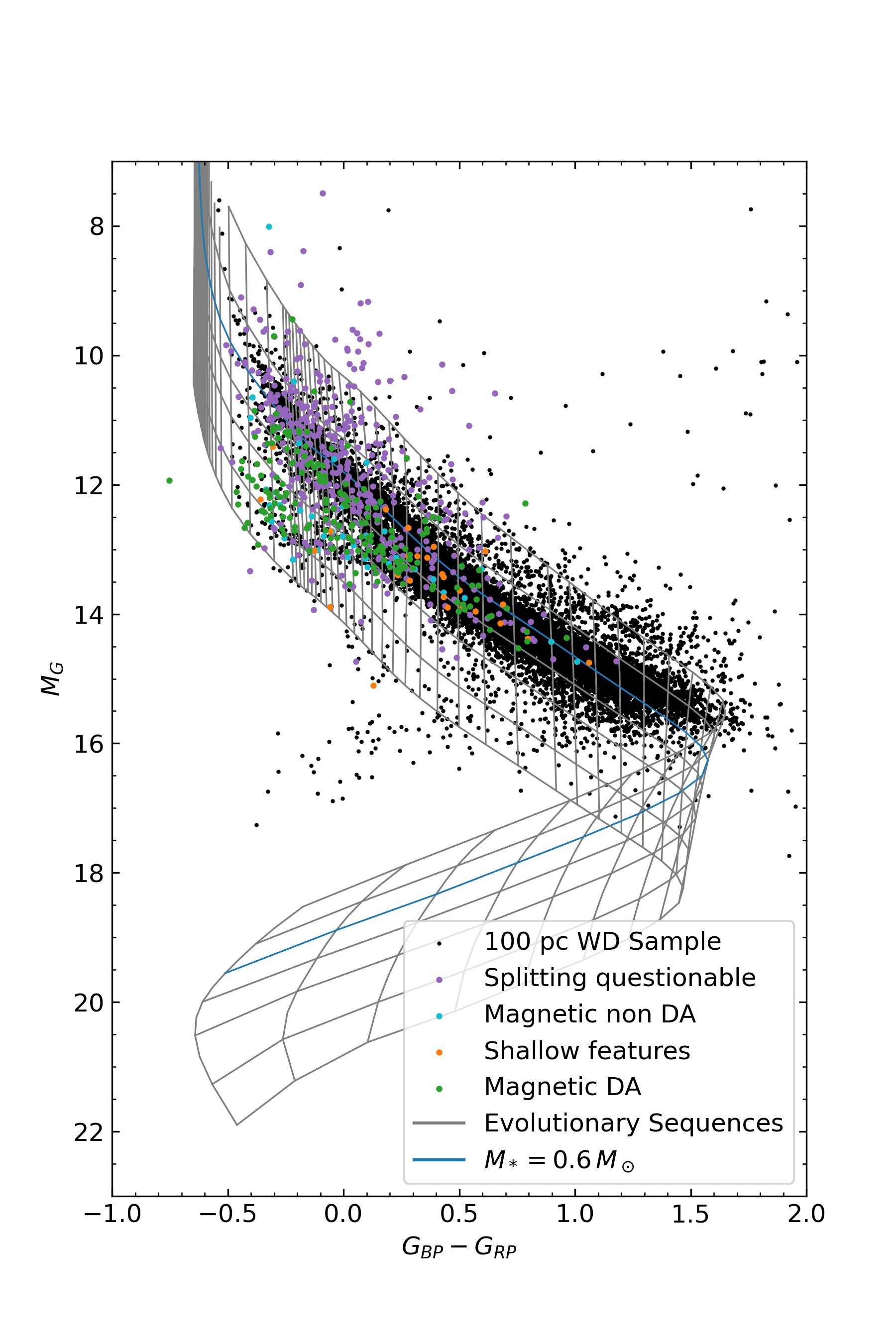
Figure 1: Gaia H-R diagram for our sample of magnetic DAs. Black dots are the white dwarfs from the Gaia EDR3 within 100 pc. The various color dots represent our full sample of 651 stars, classified into categories explained in Section 4.

2.2 Photometric and Spectroscopic Data

In order to perform an analysis as homogeneous as possible, we decided to use SDSS ugriz point-spread function magnitudes in priority when available. When ugriz data were not available, we relied on Pan-STARRS grizy or previously published JHK and BVRI photometry, in that order of priority. In the end, out of 651 objects, only 29 (4.5%) had no ugriz data. Hence we used grizy data for 26 stars and BVRI photometry for the last 3.

The majority (598 out of 651, 92%) of the spectra used for this work are collected from SDSS. The spectra of the 53 objects without SDSS spectroscopy were taken from Limoges et al. (2013, 2015), Bergeron et al. (1997, 2001), Gianninas et al. (2011), Giammichele et al. (2012), Tremblay et al. (2020) or archival data obtained by the Montreal group over the years.

2.3 Note on Naming Convention

Numerous names are often used to design a given white dwarf. In order to avoid confusion, we decided to follow a convention similar to that of Coutu et al. (2019) and use names based on ICRS coordinates at epoch and equinox 2000 (alternative names for any given star can easily be obtained through the search function on the Montreal White Dwarf Database). Stars are thus referenced with JHHMM$\pm$DDMM, where HHMM corresponds to the right ascension (R.A.) in hours and minute and DDMM to the declination (decl.) in degrees and minutes in sexagesimal notation. Table 7 provides the correspondence between the names of all objects in our sample with Gaia source ID, MWDD ID, and the coordinates in decimal format (degrees).

3 Theoretical Framework

3.1 Magnetic Synthetic Spectra Calculations

The presence of a strong magnetic field has a strong effect on both the atomic energy levels, line strengths as well as the radiative transfer as polarization has to be taken into account.

We rely on data provided by one of us (S.Jordan, similar from Forster et al., 1984; Wunner et al., 1985, 1989) which provide transitional energies, wavelengths, and various quantum quantities needed to compute oscillator strengths for a wide range of magnetic field intensities from 0 to over 9000 MG. The data used in this work were never fully published, and are denser than the ones available in the literature. As can be observed in Figure 2, line positions vary substantially in a non-linear way for fields above about 10 MG. The spectral features for objects with such strong fields can thus become much more complex than the usual Zeeman triplet found at lower fields. We implemented an interpolating scheme developed by Steffen (1990) to obtain the component data for arbitrary field intensities, with a linear extrapolation when required. This extrapolation occurs at over 9000 MG for most components, although some weaker components only have calculations up to 1000 MG. As most stars in our sample have a dipolar magnetic field $B_{p}$ of under 100 MG with only a very limited number of stars with $B_{p}$ over 500 MG, this extrapolation is not expected to be frequent. We also obtained similar data for helium transitions and implemented them into our routines. This work assumes only pure hydrogen atmospheres (other compositions will be explored in Hardy et al., in preparation).

An appropriate polarized radiative transfer routine also had to be implemented for a correct description of MWD radiation field. Jordan & Schmidt (2003) describe four methods to numerically solve the radiative transfer equations, and we decided to use their MATEXP method (Section 2.4 of their work), as it yielded smoother polarization spectra, was more numerically stable for our case, and was one of the fastest in computation time. While in principle our code is now suitable for the analysis of other Stokes parameters, we restrict our analysis to the Stokes parameter $I$ (the luminous intensity) in this work as no polarimetric data is yet available for the majority of our sample.

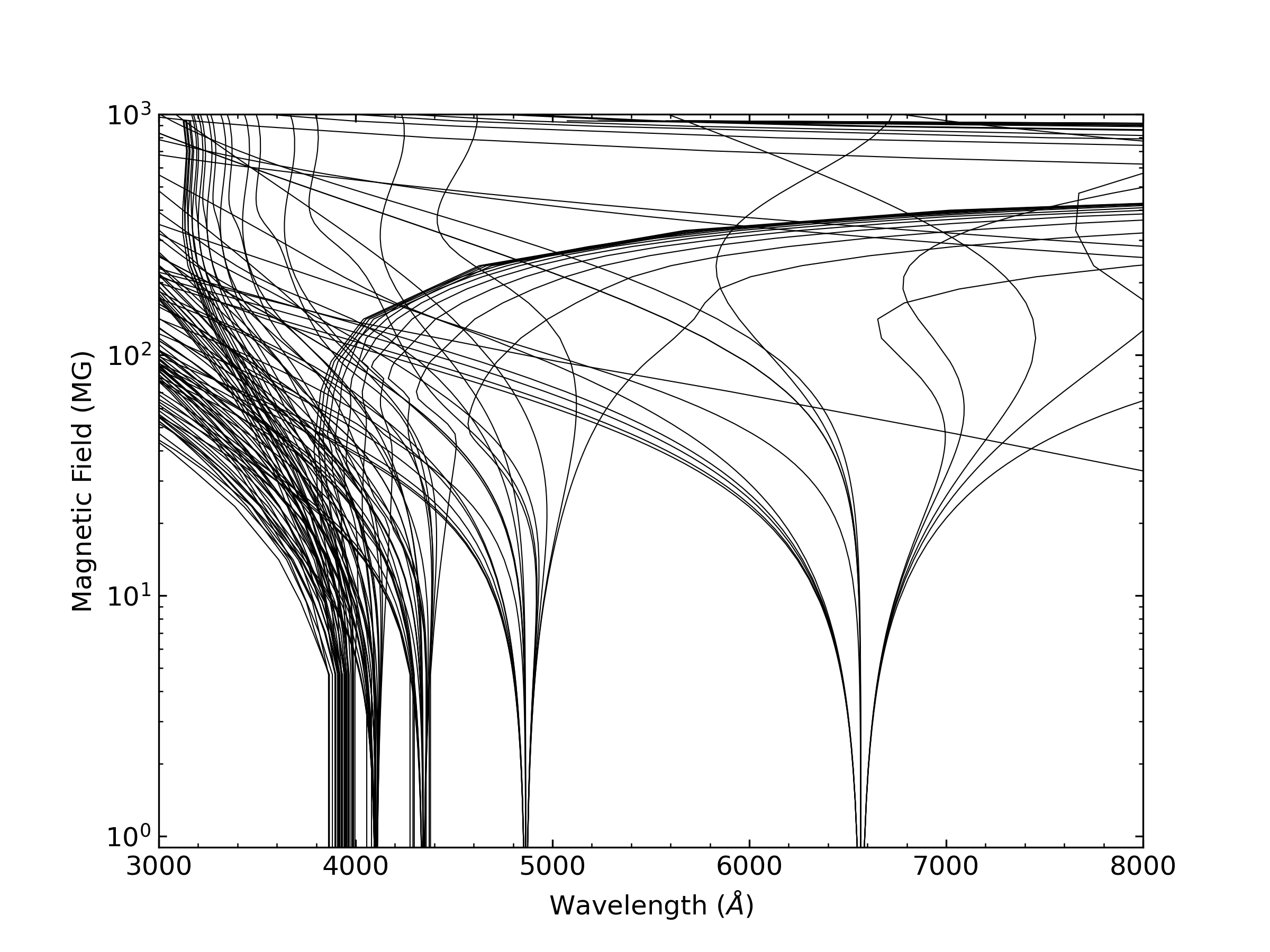
Figure 2: Position of the Balmer lines between 3000 and 8000 Å as a function of magnetic field strength.

As a first-order approximation, we model the surface magnetic field of the stars with an inclined and offset dipole:

$$\mathbf{B}=\frac{3\left(\mathbf{m}\cdot\hat{\mathbf{r}}\right)\hat{\mathbf{r}}-\mathbf{m}}{{r}^{3}}$$ (1)

where:

• $\mathbf{B}$ is the magnetic field vector, in MG,

• $\mathbf{m}=\frac{B}{2}\hat{\mathbf{m}}$ is the dipole moment vector ($B$ is the dipole intensity, in MG, $\hat{\mathbf{m}}$ the unit vector of the dipole moment),

• $\hat{\mathbf{r}}$ is the unit vector of the position vector $\mathbf{r}$, from the dipole to where the field is measured (here, the surface of the star),

• $r$ is the absolute value of the position vector $\mathbf{r}$, in stellar radii.

We orient the magnetic moment according to the inclination, and apply the dipole offset by shifting the position vector accordingly. The parameters used to describe the dipolar geometry (Figure 3) are the dipole intensity $B_{p}$, which is the magnetic field intensity at the pole of a centered dipole, at the stellar surface ($1\,R_{*}$ from the origin), the inclination angle $i$ between the dipole moment $\vec{m}$ and the observer’s line of sight, and the dipole offset $a_{z}$ (in stellar radii $R_{*}$), the distance between the center of the dipole and the center of the star.

We discretize the stellar surface into many surface elements. The number of surface element has to be large enough to correctly sample the variation of the magnetic field on the surface, but not too large as to slow down the calculation significantly. We find that using 149 surface elements was optimal as no significant change to the computed synthetic spectra were found in tests using a finer resolution. Once the specific intensity for each surface element has been calculated, we integrate across the stellar surface to obtain the Eddington flux for any given geometry.

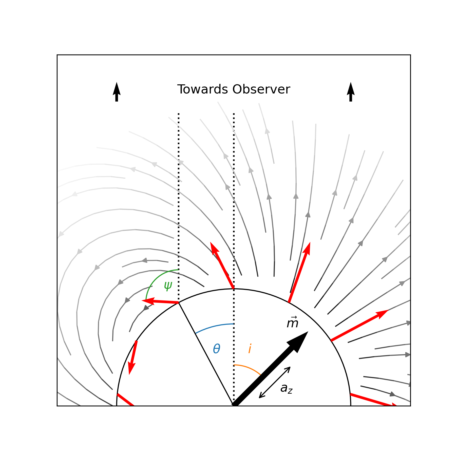
Figure 3: Schema for the various parameters describing our dipole geometry. In red are the magnetic field vectors at the stellar surface, with the angle $\psi$ in green and $\theta$ in blue used to model each surface elements. $\vec{m}$, the inclination angle $i$ and dipole offset $a_{z}$ describe the geometry of the field.

In order to recover the magnetic field geometry for every star in our sample, a significant number of synthetic spectra across a wide range of effective temperatures, surface gravity, and geometries were required. Pre-generating all the necessary dipolar-geometry intensity spectra would have been much more time consuming (and less expandable in the future) than integrating them on-the-fly using a precomputed grid of spectra with a constant field. We therefore built a spectrum grid across 5 parameters: effective temperature (5000 K to 30,000 K in 15 steps), surface gravity ($\log{g}$ from 7.0 to 9.5 in 6 steps), field intensity ($10^{-2}$ MG to $10^{4}$ MG in 159 steps), the angle between the line of sight and the normal of the surface ($\psi$ from 0 to $\pi$ in 6 steps), and the limb darkening ($\mu=\cos{\theta}$ from 0 to 1 in 4 steps). From this precomputed grid (85 GB of data), a synthetic spectrum with any desired field strength and geometry (not limited to offset dipole) can be reconstructed rapidly. Only offset dipole geometries are considered in this exploratory work.

3.2 Photometric Analysis Technique

The first step in our analysis is to estimate the effective temperature and surface gravity of our objects. However, the presence of a strong magnetic field can affect significantly the determination of these atmospheric parameters. As a start, we first obtained effective temperature and surface gravity with models with no magnetic field. The atmospheric structures and synthetic colors used are those of Bergeron et al. (2019) (same atmospheric models used by Genest-Beaulieu & Bergeron, 2019). Note that those models do not include the effect of magnetism on the stellar structure. In fact, it is not clear at the moment how exactly the structure is affected by the presence of a strong magnetic field and as a consequence, all past studies, to our knowledge, used non-magnetic structure to calculate magnetic synthetic spectra (see Külebi et al., 2009, for example). We thus employed a similar strategy here but improved on the fitting technique by including explicitly the effect of magnetism when determining atmospheric parameters from photometric data (see below).

We obtain the effective temperature and surface gravity with zero-field models using an evolutionary algorithm (based on Storn & Price, 1997) to fully explore the parameter space of the grid (this is a test to make sure we recover the non-magnetic parameters obtained with standard technique before proceeding with magnetic synthetic spectra). We applied de-reddening corrections to the observed magnitudes to take into account the amount of interstellar material on the line of sight (Schlafly & Finkbeiner, 2011). We then constructed new synthetic grids with various magnetic field strengths to account for the shifting of lines from one photometric band to the other as the field increases. The atmosphere structures are the same as those used previously but the synthetic spectrum used to derive the synthetic photometric colors include the effect of the magnetic field on the line splitting. With these photometric grids in hand, we proceeded to obtain a value for the atmospheric parameters for every star in our sample for field strength of 0, 10, 50, 100, 500, 700, and 900 MG. For each star in our sample, we built an interpolating table for the atmospheric parameters (effective temperature, surface gravity), plus mass and radius, so we can get interpolated values for arbitrary magnetic field intensities that will be obtained in the next step. While this is done assuming a constant surface magnetic field, this method allows to at least capture the main effect of the presence of strong magnetic fields, that is the shifting of lines in adjacent bands (the exact details of the geometry is a second-order effect in that matter).

Figure 4 shows how the synthetic ugriz colors are affected by the inclusion of magnetic splitting for various field strength and effective temperatures. In the case of magnetic DA stars, the u and g bands are the most affected, since the Balmer lines (except H$\alpha$) are near them. With weak or no magnetic field, there are barely any Balmer lines in the u band, but a magnetic field with an intensity above a few MG pushes many components inside the band. A similar phenomenon happens for the g band, which is in the range of the Balmer lines starting from H$\beta$. Here the many split components affect the g band considerably. With increased magnetic field, the r band is the least affected as H$\alpha$ components tend to stay inside the band and the i band can only have H$\alpha$ components drift inside. The z band is a little different, since some of the Paschen lines are not split in our model, due to a lack of data.

Including the effect of magnetism in the synthetic spectra can thus have a non-negligible effect on the atmospheric parameter determination (effective temperature and surface gravity). This is the first time, to our knowledge, that this effect is explicitly taken into account for the determination of the atmospheric parameters. Uncertainties on the fitted values were obtained by fitting the photometry again, but with a least-squares minimization method that also returns the estimated uncertainties. We used the values obtained with the fitting method described above as starting values for the algorithm, ensuring uncertainties around those values.

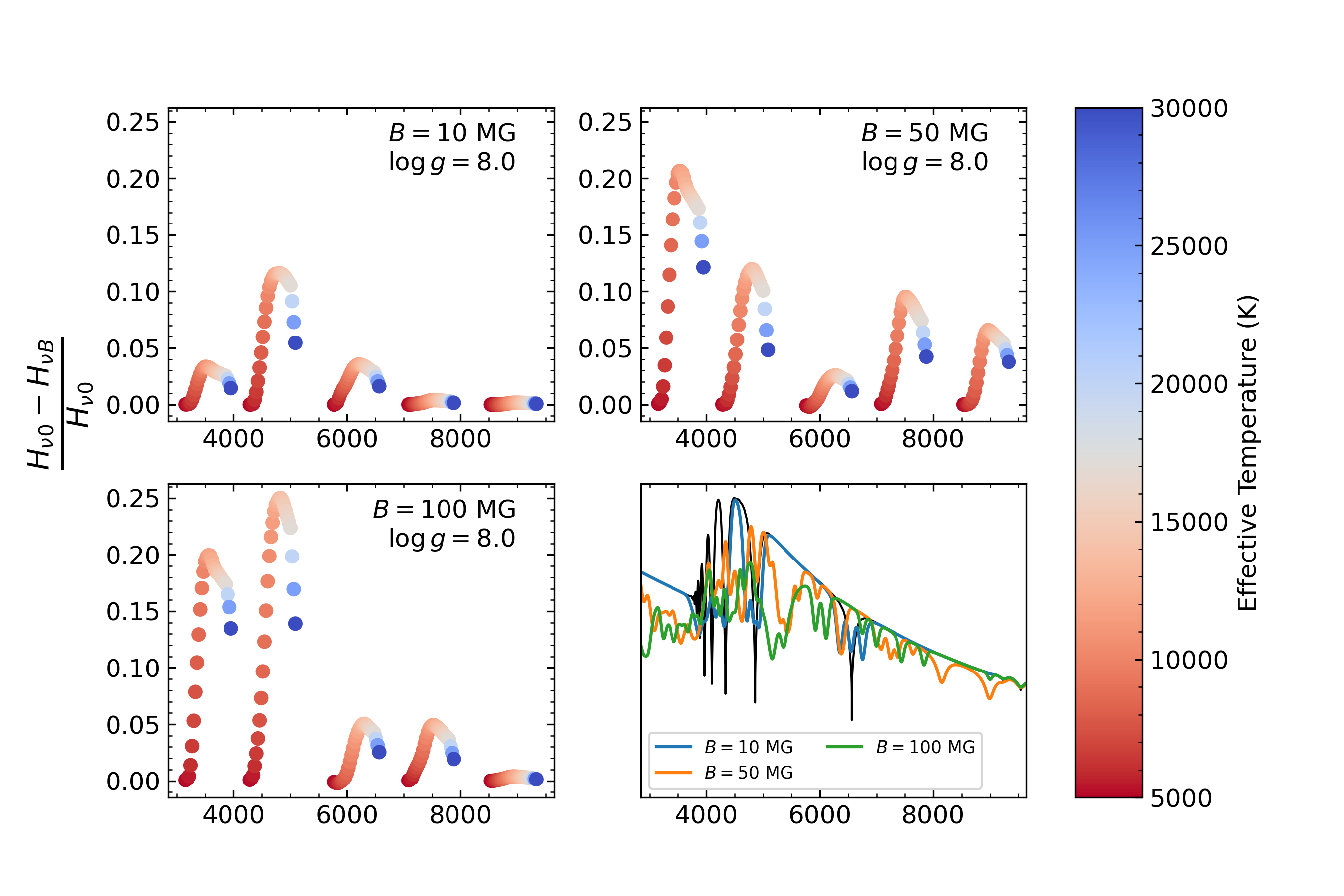
Figure 4: Relative differences in magnitude for models with and without magnetic field.

3.3 Spectroscopic Analysis Technique

When fitting a given star, the process to obtain a synthetic geometry-aware spectrum is the following:

• Provide the dipole geometry parameters: $B_{p}$, $i$, $a_{z}$;

• Generate an $N$-element discretized surface geometry and compute the average surface field intensity;

• Interpolate the effective temperature and surface gravity to that average field value;

  • See previous Section 3.2.

• Use those atmospheric parameters with each surface element to obtain the $N$ spectrum elements by interpolating in the 5-D grid;

• Sum the $N$ spectra into the dipolar-geometry-aware spectrum at the desired atmospheric parameters.

We use this process in the fitting technique to obtain every spectrum needed for each iteration until convergence. Due to the high dimensionality of the problem and the highly degenerate nature of the solutions, standard minimization methods using the gradient descent are ill suited for this situation, since many local minima are found with different dipolar geometry. The usual steepest-descent algorithm would get stuck on the first minimum it would encounter based on an initial guess value. Making this initial guess value would be different for each star and is not optimal. This is why the optimization algorithm used relies on a stochastic nature and allows searching for a wide area inside the parameter space. It is part of the scipy Python package, which is an implementation of the algorithm by Storn & Price (1997).

We tested our method by generating non-magnetic and magnetic synthetic stars with various magnetic field intensities and geometries and fed it to our fitting code. Our algorithm was able to retrieve the geometry for both the magnetic and the non-magnetic stars with satisfactory precision. For the special case of non-magnetic synthetic stars, we still used the algorithm to get a dipolar geometry, but the dipolar intensity from the solution is minimal and the other parameters (angle and offset) are less constrained and are of no physical value.

Typical uncertainties were estimated by changing the dipole parameters ($B_{p}$, $i$, $a_{z}$) until the resulting synthetic spectrum diverged significantly from the observations, for a typical magnetic star in our sample. We observed that the relative uncertainties for the different parameters were very different, meaning the solutions were more sensitive to an increase of magnetic field intensity ($B_{p}$) than the other geometry parameters. We found a relative uncertainty of 5% for the $B_{p}$ parameter, 20% for the inclination $i$, and 50% for the dipole offset $a_{z}$.

In summary, the fitting technique for magnetic spectra begins with the creation of a random set of ($B_{p}$, $i$, $a_{z}$) parameters. For each individual in this population, we go through the process described above to obtain a spectrum, and calculate the $\chi^{2}$ value against the observations.

4 Spectrophotometric Analysis

Using the fitting technique described in Section 3, we fitted all 651 objects in our sample in a homogeneous way assuming single DA synthetic spectra with a dipolar geometry. Each solution was then carefully inspected by eye to judge the quality of the fit. As a result of this laborious exercise, we could classify all our objects in broadly 5 categories (see Table 1): i) stars that are probably not magnetic (400) ii) stars well fitted with a dipole geometry (140) iii) stars that are clearly hydrogen-rich magnetic white dwarfs but that are moderately well modeled with a dipolar geometry (45) iv) stars that have hydrogen features too shallow (28) and finally v) stars that we were simply unable to fit using the current theoretical framework (38). We now discuss each category in turn.

Table 1: Numbers of stars in our different categories

Category	Subcategory	Count
Magnetic DA	Good dipole fit	140	185
	Bad dipole fit	45
Dismissed stars	Magnetic non DA / Unable to fit	38	466
	Shallow features	28
	Splitting questionable	400
Total		651

The first category contains more than half of our original sample (400 stars). Most of these object had been classified as DAH or DAH: from visual classification of low signal-to-noise ratio spectra from various data release catalog of spectroscopically confirmed white dwarf stars from the Sloan Digital Sky Survey (Kleinman et al., 2004, 2013; Kepler et al., 2015, 2019). While visual inspection indeed seems to show possible shifted components near the core of some Balmer lines (thus the DAH classification), it quickly became clear that those classifications did not hold up against detailed comparison with magnetic synthetic spectra. For example, it was possible in a few cases to force a magnetic field strength/geometry to fit some glitches near the core of one Balmer line only to find that such configuration lead to predicted components that are not observed in the other lines. When considering all the lines simultaneously, our algorithm was not able to find a magnetic solution that was statistically better than a non-magnetic fit. In the end, although it is quite possible that some of these stars will be found to be genuinely magnetic white dwarfs when higher signal-to-noise or spectropolarimetric observations become available, we believe that classifying these objects as DAH based on these low quality SDSS spectra was perhaps a bit premature. We report in Table 2 the photometric atmospheric parameters (effective temperature and $\log{g}$) assuming $B=0$ and reassign them with the spectral type DA until proof to the contrary.

Table 2: Stars with no compelling evidence of magnetism

J name	$T_{\rm{eff}}$ (K)	$\log{g}$	Mass ($M_{\odot}$)
J0002$-$4310	8979 (328)	8.49 (0.3)	0.912 (0.38)
J0003$-$0153	15408 (638)	8.49 (0.17)	0.918 (0.18)
J0005+1934	5367 (248)	7.57 (0.11)	0.360 (0.074)
J0007+2407	7653 (660)	7.27 (0.25)	0.268 (0.14)
J0010+2429	6247 (46)	7.74 (0.76)	0.448 (0.072)
J0012+5025	6354 (27)	8.23 (0.031)	0.735 (0.041)
J0016+2350	12296 (378)	9.09 (0.61)	1.233 (0.56)
J0040+0702	16927 (454)	8.61 (0.17)	0.997 (0.22)
J0040+2438	14715 (325)	8.15 (0.25)	0.700 (0.3)
J0042+2358	10291 (374)	7.71 (0.84)	0.446 (0.071)
J0054+1202	19449 (276)	7.91 (0.088)	0.574 (0.095)
J0101$-$0411	16819 (122)	8.03 (0.016)	0.636 (0.019)
J0103+1511	18175 (375)	7.74 (0.25)	0.486 (0.19)
J0104+1459	14144 (358)	7.75 (0.96)	0.480 (0.081)
J0109+1800	15273 (618)	8.53 (0.42)	0.944 (0.5)
J0111+1410	14365 (262)	7.78 (0.25)	0.495 (0.2)
J0112+2653	12234 (358)	8.74 (0.31)	1.069 (0.34)
J0117+2422	15318 (164)	8.18 (0.22)	0.723 (0.22)
J0117+3035	18623 (409)	$<$7.00 (0.25)	0.264 (0.11)
J0121+3210	16677 (702)	8.66 (0.22)	1.026 (0.44)
J0121+3932	20972 (332)	7.92 (0.25)	0.581 (0.23)
J0122+0827	9498 (320)	8.29 (0.25)	0.781 (0.41)
J0125$-$1013	11503 (482)	8.18 (0.25)	0.717 (0.35)
J0126+1934	6994 (47)	8.21 (0.14)	0.723 (0.12)
J0137+2351	15156 (385)	7.56 (0.25)	0.397 (0.15)
J0138+2523	30000 (0)	8.83 (0.15)	1.128 (0.14)
J0143+1437	9444 (549)	7.58 (0.25)	0.386 (0.14)
J0143$-$1015	16777 (118)	9.00 (0.94)	1.199 (1)
J0148$-$0048	10818 (1000)	7.99 (0.25)	0.596 (0.32)
J0203+2205	10605 (938)	8.19 (0.25)	0.722 (0.31)
J0205+0030	14395 (445)	7.57 (0.25)	0.399 (0.17)
J0207+2238	6642 (121)	7.86 (0.2)	0.512 (0.14)
J0211+0722	13914 (1642)	7.35 (0.25)	0.320 (0.14)
J0213+0530	9361 (490)	7.21 (0.25)	0.264 (0.13)
J0218+0355	7719 (62)	8.46 (0.13)	0.890 (0.13)
J0230+2508	5476 (32)	7.86 (0.23)	0.503 (0.26)
J0231+2648	9518 (269)	8.54 (0.16)	0.941 (0.18)
J0235+2416	13691 (448)	7.27 (0.25)	0.298 (0.13)
J0242+2916	18927 (259)	8.17 (0.24)	0.723 (0.3)
J0249+3327	15594 (359)	7.25 (0.25)	0.302 (0.12)
J0250+3414	21791 (845)	9.13 (0.16)	1.251 (0.36)
J0259+0811	6344 (75)	7.77 (0.12)	0.460 (0.12)
J0301+0539	20367 (661)	9.09 (0.12)	1.235 (0.16)
J0305+0502	13028 (442)	8.30 (0.22)	0.793 (0.26)
J0305+3707	11800 (624)	7.84 (0.25)	0.519 (0.23)
J0307+3628	8112 (222)	8.88 (0.15)	1.139 (0.21)
J0310+0451	13551 (440)	8.10 (0.25)	0.671 (0.3)
J0319+4103	16592 (224)	7.99 (0.25)	0.608 (0.26)
J0326+0403	19345 (298)	9.04 (0.73)	1.217 (0.7)
J0340$-$0635	20306 (297)	9.18 (0.79)	1.267 (0.85)
J0343$-$0044	6802 (353)	$<$7.00 (0.25)	0.195 (0.12)
J0344$-$0514	14214 (894)	8.74 (0.23)	1.073 (0.45)
J0346+0948	22030 (464)	9.11 (0.13)	1.243 (0.091)
J0347+1000	11173 (381)	8.82 (0.12)	1.113 (0.15)
J0350+0858	13075 (265)	7.54 (0.25)	0.385 (0.16)
J0357$-$0439	11269 (835)	7.71 (0.19)	0.452 (0.12)
J0443+1131	16248 (690)	7.79 (0.25)	0.501 (0.2)
J0445$-$0525	13246 (526)	8.39 (0.25)	0.850 (0.44)
J0446+1015	8285 (355)	7.98 (0.14)	0.583 (0.11)
J0452+2519	20967 (144)	8.17 (0.00041)	0.728 (0.001)
J0534+6254	9517 (232)	8.19 (0.25)	0.719 (0.34)
J0535+0016	21389 (799)	9.30 (0.93)	1.302 (0.13)
J0641+4744	13707 (137)	8.23 (0.014)	0.753 (0.019)
J0645+2803	12648 (338)	7.97 (0.24)	0.589 (0.24)
J0714+4012	19637 (705)	$<$7.00 (0.25)	0.268 (0.11)
J0716+3935	16278 (503)	8.15 (0.56)	0.705 (0.65)
J0727+4036	13516 (336)	8.85 (0.1)	1.127 (0.11)
J0730+3627	14654 (499)	8.12 (0.23)	0.681 (0.24)
J0731+3531	21933 (490)	7.72 (0.25)	0.488 (0.19)
J0733+6409	5007 (29)	7.76 (0.085)	0.447 (0.088)
J0735+6526	15263 (1201)	7.24 (0.25)	0.298 (0.12)
J0738+2236	16602 (528)	8.28 (0.25)	0.788 (0.38)
J0746+1538	21149 (314)	7.21 (0.25)	0.318 (0.12)
J0746+2818	14333 (584)	8.70 (0.23)	1.046 (0.45)
J0749+1545	22303 (624)	8.01 (0.23)	0.633 (0.22)
J0750+2220	15003 (1791)	8.88 (0.19)	1.145 (0.38)
J0752+2831	13793 (631)	8.17 (0.25)	0.715 (0.32)
J0756+1427	16919 (821)	8.09 (0.25)	0.672 (0.3)
J0757+0855	15712 (2553)	8.76 (0.18)	1.082 (0.26)
J0758+1214	13099 (194)	8.25 (0.14)	0.763 (0.12)
J0758+1439	19008 (1544)	8.11 (0.25)	0.687 (0.33)
J0800+8327	15446 (297)	7.81 (0.25)	0.509 (0.21)
J0801+0643	30000 (0)	7.72 (0.25)	0.512 (0.18)
J0802+1530	12218 (514)	8.19 (0.22)	0.719 (0.22)
J0806$-$0754	11091 (786)	9.45 (0.45)	1.346 (0.42)
J0807+1355	12703 (467)	8.05 (0.25)	0.636 (0.29)
J0809+0624	18295 (280)	7.38 (0.25)	0.349 (0.14)
J0809+1741	28066 (584)	8.23 (0.25)	0.775 (0.35)
J0812+1317	18353 (224)	8.00 (0.2)	0.620 (0.15)
J0812+1825	15825 (546)	8.45 (0.23)	0.895 (0.37)
J0812+5039	14952 (305)	8.46 (0.12)	0.898 (0.11)
J0813+2621	21916 (1543)	7.06 (0.25)	0.287 (0.11)
J0814+5037	21155 (843)	8.18 (0.22)	0.735 (0.21)
J0814$-$0052	16603 (744)	8.10 (0.25)	0.673 (0.29)
J0815+0843	13717 (472)	7.03 (0.25)	0.245 (0.11)
J0816+5226	7108 (92)	8.01 (0.4)	0.600 (0.46)
J0817+1543	17225 (624)	8.24 (0.22)	0.761 (0.24)
J0821+1944	26778 (771)	7.52 (0.25)	0.425 (0.15)
J0823+4013	17654 (67)	8.03 (0.25)	0.633 (0.27)
J0824+1315	18369 (260)	7.20 (0.25)	0.302 (0.12)
J0828+1817	13360 (378)	7.68 (0.25)	0.445 (0.18)
J0829+1009	15340 (710)	8.56 (0.17)	0.963 (0.19)
J0830+1858	21648 (976)	8.83 (0.14)	1.124 (0.18)
J0832$-$0428	9675 (661)	8.04 (0.25)	0.621 (0.29)
J0833+2348	10447 (929)	8.78 (0.21)	1.088 (0.37)
J0834+1317	14344 (470)	7.87 (0.25)	0.537 (0.22)
J0834+1605	16466 (526)	$<$7.00 (0.25)	0.254 (0.11)
J0834+2525	23241 (1540)	7.04 (0.25)	0.290 (0.11)
J0834+3049	17132 (167)	7.33 (0.25)	0.329 (0.13)
J0836+1034	20414 (1110)	7.99 (0.18)	0.621 (0.13)
J0836+4420	9515 (545)	7.36 (0.25)	0.306 (0.13)
J0837+1544	17207 (276)	8.31 (0.21)	0.808 (0.25)
J0838+0925	17715 (426)	8.57 (0.24)	0.975 (0.44)
J0839+2121	10179 (189)	8.45 (0.22)	0.885 (0.31)
J0840+0942	9123 (207)	7.93 (0.17)	0.556 (0.12)
J0840+1257	11804 (126)	7.91 (0.25)	0.551 (0.24)
J0841+1549	14549 (574)	8.56 (0.25)	0.962 (0.45)
J0842+1018	13610 (153)	8.31 (0.12)	0.800 (0.11)
J0843+0628	22236 (318)	8.17 (0.1)	0.726 (0.097)
J0845+1124	11935 (394)	8.12 (0.25)	0.680 (0.32)
J0845+1500	17978 (325)	7.04 (0.25)	0.267 (0.11)
J0845+3129	9180 (379)	8.40 (0.25)	0.850 (0.46)
J0848+2140	19217 (256)	7.87 (0.25)	0.553 (0.23)
J0849+2247	18622 (932)	8.21 (0.25)	0.748 (0.37)
J0850+1505	8249 (940)	7.70 (0.25)	0.436 (0.19)
J0851+1952	9131 (339)	8.49 (0.77)	0.913 (0.83)
J0851+3531	7283 (78)	8.29 (0.1)	0.779 (0.1)
J0853+1804	12624 (216)	7.48 (0.25)	0.359 (0.15)
J0855+2417	9430 (314)	7.89 (0.25)	0.533 (0.22)
J0858+1037	17722 (267)	7.96 (0.13)	0.596 (0.1)
J0858+4715	20425 (373)	7.85 (0.86)	0.546 (0.08)
J0900+2045	18926 (2166)	8.06 (0.21)	0.656 (0.21)
J0901+0640	6550 (45)	8.43 (0.44)	0.870 (0.55)
J0902+4549	11115 (204)	8.07 (0.086)	0.642 (0.11)
J0903+2226	14044 (522)	8.18 (0.25)	0.717 (0.33)
J0905+2057	13258 (277)	7.80 (0.25)	0.500 (0.21)
J0905+2138	25453 (434)	7.53 (0.25)	0.421 (0.15)
J0907+5559	13961 (709)	8.54 (0.57)	0.950 (0.65)
J0908+0105	7155 (44)	7.82 (0.22)	0.489 (0.16)
J0909+0944	14380 (401)	8.48 (0.67)	0.911 (0.75)
J0909+1938	10648 (196)	8.14 (0.25)	0.689 (0.32)
J0909+2508	10955 (209)	8.56 (0.71)	0.960 (0.77)
J0910+0815	27522 (604)	7.98 (0.71)	0.629 (0.071)
J0910+2322	15712 (279)	7.80 (0.25)	0.508 (0.21)
J0910+2501	14638 (207)	7.10 (0.25)	0.263 (0.12)
J0911+2232	11109 (241)	8.10 (0.23)	0.662 (0.23)
J0912+1026	22618 (322)	7.55 (0.25)	0.421 (0.15)
J0913+1141	14235 (634)	8.25 (0.21)	0.767 (0.21)
J0913+1739	13807 (333)	7.52 (0.25)	0.380 (0.15)
J0915+2050	10648 (263)	7.57 (0.25)	0.385 (0.17)
J0916+1248	15451 (293)	7.67 (0.25)	0.447 (0.18)
J0916+2150	5486 (76)	7.98 (0.71)	0.572 (0.077)
J0917+0112	17473 (335)	8.39 (0.16)	0.856 (0.15)
J0917+6014	13976 (664)	8.55 (0.016)	0.959 (0.022)
J0918+0648	23436 (719)	7.98 (0.2)	0.619 (0.15)
J0921+1301	12979 (555)	8.40 (0.19)	0.857 (0.21)
J0923+2435	14247 (674)	7.01 (0.25)	0.245 (0.11)
J0924+2318	7535 (75)	8.12 (0.14)	0.666 (0.12)
J0928+2454	13328 (903)	$<$7.00 (0.25)	0.238 (0.11)
J0929+0135	14799 (513)	8.34 (0.19)	0.823 (0.19)
J0929+1554	17559 (3)	9.49 (0.46)	1.363 (0.47)
J0930+2024	11385 (862)	8.18 (0.18)	0.711 (0.15)
J0935+0008	16196 (475)	8.11 (0.18)	0.679 (0.14)
J0936+1829	12000 (334)	8.39 (0.25)	0.849 (0.45)
J0937+2057	12109 (538)	8.57 (0.21)	0.967 (0.32)
J0938+6156	15386 (696)	8.45 (0.22)	0.898 (0.31)
J0940+6314	14965 (205)	8.39 (0.22)	0.855 (0.28)
J0942+1838	17522 (127)	$<$7.00 (0.25)	0.259 (0.11)
J0942+5213	8119 (42)	7.94 (0.16)	0.561 (0.12)
J0945+4226	21458 (893)	7.37 (0.25)	0.359 (0.14)
J0948+2421	20419 (174)	8.43 (0.013)	0.888 (0.016)
J0949+4827	19642 (955)	7.59 (0.25)	0.426 (0.16)
J0949+4956	13041 (545)	8.38 (0.06)	0.847 (0.08)
J0957$-$0123	25118 (787)	7.34 (0.25)	0.366 (0.13)
J1000+3047	14042 (347)	9.06 (0.53)	1.224 (0.46)
J1004+2238	10614 (781)	7.09 (0.25)	0.242 (0.12)
J1006+1442	12123 (392)	8.10 (0.25)	0.667 (0.29)
J1007+2814	10483 (457)	8.59 (0.19)	0.976 (0.25)
J1014+5949	6812 (74)	7.59 (0.73)	0.377 (0.059)
J1015+4415	6823 (109)	8.71 (0.11)	1.044 (0.12)
J1016+2816	22129 (361)	8.26 (0.25)	0.785 (0.37)
J1022+1446	7917 (140)	8.63 (0.65)	1.000 (0.72)
J1024+4107	17014 (216)	7.87 (0.14)	0.545 (0.1)
J1025+2820	21696 (591)	7.99 (0.25)	0.622 (0.25)
J1027+4351	13679 (348)	7.52 (0.25)	0.378 (0.15)
J1028+1451	5538 (29)	7.82 (0.038)	0.480 (0.041)
J1034+3050	14502 (231)	8.13 (0.23)	0.689 (0.26)
J1036+1710	13543 (306)	7.63 (0.25)	0.421 (0.17)
J1041+0918	11220 (356)	8.34 (0.23)	0.820 (0.34)
J1041+0945	7419 (216)	7.26 (0.25)	0.265 (0.13)
J1041+4043	6493 (26)	7.02 (0.12)	0.198 (0.051)
J1043$-$0125	22540 (823)	7.81 (0.25)	0.528 (0.21)
J1044+0942	16627 (425)	8.72 (0.22)	1.063 (0.45)
J1047+3108	8304 (110)	8.41 (0.2)	0.859 (0.25)
J1050+1433	21902 (545)	7.29 (0.25)	0.339 (0.12)
J1051+3211	15223 (352)	8.71 (0.16)	1.056 (0.23)
J1055+2111	5850 (90)	8.04 (0.14)	0.610 (0.17)
J1055+3604	15283 (431)	$<$7.00 (0.25)	0.248 (0.11)
J1057+4801	16781 (637)	8.92 (0.16)	1.166 (0.27)
J1058+3422	11659 (375)	7.88 (0.25)	0.535 (0.23)
J1058+3724	11561 (415)	8.43 (0.9)	0.874 (0.093)
J1058+5731	16592 (885)	8.39 (0.62)	0.855 (0.72)
J1102+4005	9477 (274)	8.61 (0.11)	0.991 (0.11)
J1107$-$1506	17319 (318)	8.29 (0.25)	0.797 (0.39)
J1107$-$1607	15966 (254)	9.02 (0.068)	1.207 (0.056)
J1112+1857	8953 (160)	8.64 (0.15)	1.004 (0.17)
J1120+4004	14086 (542)	8.93 (0.84)	1.167 (0.85)
J1124+2624	12696 (462)	8.08 (0.25)	0.657 (0.29)
J1128$-$0105	12825 (1128)	7.44 (0.011)	0.347 (0.016)
J1131+3550	17170 (348)	8.14 (0.1)	0.703 (0.099)
J1132+0640	19466 (87)	7.60 (0.22)	0.431 (0.13)
J1134+1822	8262 (278)	8.72 (0.14)	1.051 (0.17)
J1135+2912	19650 (660)	8.45 (0.25)	0.903 (0.44)
J1137+3254	20861 (793)	7.09 (0.25)	0.289 (0.11)
J1145+3008	15458 (281)	7.90 (0.25)	0.559 (0.23)
J1148+1533	11819 (391)	8.73 (0.19)	1.062 (0.33)
J1148+3039	11944 (331)	8.23 (0.25)	0.750 (0.37)
J1149+3000	10255 (147)	7.36 (0.16)	0.308 (0.095)
J1156+3531	16172 (602)	8.46 (0.25)	0.900 (0.45)
J1159+0007	9706 (126)	8.71 (0.065)	1.051 (0.076)
J1207+4407	18787 (950)	8.10 (0.19)	0.682 (0.16)
J1208+1449	12707 (307)	$<$7.00 (0.25)	0.235 (0.11)
J1209+3317	6591 (13)	7.43 (0.9)	0.315 (0.061)
J1210+2330	17134 (72)	8.04 (0.41)	0.638 (0.46)
J1210+5243	15637 (495)	8.49 (0.15)	0.921 (0.18)
J1211+0204	9875 (199)	8.37 (0.078)	0.832 (0.1)
J1212+1852	21847 (890)	7.60 (0.25)	0.437 (0.16)
J1215+3351	17533 (410)	8.00 (0.22)	0.619 (0.19)
J1217+1728	23956 (633)	7.07 (0.25)	0.300 (0.11)
J1222+0050	11689 (324)	$<$7.00 (0.25)	0.230 (0.11)
J1223+2553	15360 (1154)	8.54 (0.1)	0.952 (0.1)
J1225+1923	16111 (641)	7.63 (0.2)	0.432 (0.12)
J1231+2419	20157 (426)	7.77 (0.25)	0.505 (0.2)
J1235+1453	15072 (235)	$<$7.00 (0.25)	0.247 (0.11)
J1235$-$0535	16716 (149)	8.36 (0.039)	0.836 (0.05)
J1240+0636	15419 (117)	7.93 (0.12)	0.577 (0.1)
J1240+4000	13795 (653)	8.30 (0.25)	0.797 (0.38)
J1243+1513	7016 (58)	7.84 (0.89)	0.501 (0.086)
J1247+0009	8432 (64)	8.04 (0.25)	0.620 (0.29)
J1248+1335	13409 (319)	8.22 (0.19)	0.744 (0.16)
J1248+4110	17660 (211)	7.87 (0.18)	0.548 (0.12)
J1251+3519	19996 (461)	8.50 (0.1)	0.933 (0.099)
J1254+0921	8279 (264)	8.42 (0.23)	0.867 (0.33)
J1254+4918	6492 (29)	8.29 (0.21)	0.775 (0.27)
J1255+1525	15113 (612)	7.41 (0.25)	0.344 (0.14)
J1255+1549	13336 (181)	7.54 (0.25)	0.383 (0.16)
J1258+2338	8197 (146)	8.33 (0.21)	0.803 (0.28)
J1305+2830	27824 (507)	7.97 (0.25)	0.628 (0.25)
J1308+0354	17571 (345)	7.75 (0.84)	0.486 (0.074)
J1309+0106	16196 (538)	7.80 (0.25)	0.507 (0.21)
J1314+0632	16668 (635)	8.35 (0.11)	0.835 (0.11)
J1315+2623	8612 (123)	8.32 (0.12)	0.799 (0.11)
J1317+2818	12550 (372)	7.51 (0.18)	0.369 (0.11)
J1318+0717	18823 (436)	7.15 (0.25)	0.291 (0.12)
J1319+0152	17351 (630)	7.43 (0.77)	0.361 (0.046)
J1320+1319	15452 (276)	7.13 (0.25)	0.273 (0.12)
J1324+2935	15582 (703)	8.54 (0.49)	0.953 (0.58)
J1325+5151	9358 (38)	7.76 (0.25)	0.468 (0.2)
J1328+0423	12966 (854)	8.49 (0.08)	0.917 (0.1)
J1330+2248	15351 (238)	8.25 (0.24)	0.769 (0.31)
J1331+1240	20248 (388)	7.95 (0.12)	0.596 (0.099)
J1337+0724	18052 (233)	7.81 (0.86)	0.520 (0.078)
J1339+1705	15879 (409)	8.25 (0.25)	0.767 (0.38)
J1340+3250	24230 (550)	7.93 (0.11)	0.593 (0.095)
J1347+1021	6914 (52)	8.00 (0.083)	0.593 (0.099)
J1351+0743	13344 (257)	8.81 (0.49)	1.108 (0.5)
J1352+1120	15618 (427)	7.93 (0.24)	0.573 (0.23)
J1353$-$0916	8736 (47)	8.32 (0.033)	0.800 (0.044)
J1400+3307	21398 (530)	7.75 (0.25)	0.500 (0.19)
J1404+2019	14038 (208)	7.78 (0.16)	0.494 (0.11)
J1413+1918	18066 (263)	9.05 (0.12)	1.222 (0.091)
J1416+2354	17786 (265)	8.17 (0.2)	0.719 (0.25)
J1417+5735	5373 (79)	8.12 (0.31)	0.656 (0.39)
J1418+4818	13675 (293)	7.33 (0.15)	0.315 (0.085)
J1419+2543	9279 (132)	8.40 (0.025)	0.856 (0.033)
J1420+1039	15431 (263)	8.02 (0.11)	0.625 (0.099)
J1420+1120	17701 (301)	8.23 (0.19)	0.760 (0.18)
J1427+1009	17068 (306)	7.74 (0.95)	0.483 (0.08)
J1428+3908	8839 (413)	8.45 (0.25)	0.882 (0.46)
J1430+2848	16034 (210)	7.63 (0.13)	0.428 (0.093)
J1431+0121	16166 (316)	7.93 (0.17)	0.575 (0.12)
J1432+4301	24172 (1042)	7.92 (0.17)	0.588 (0.12)
J1435+0729	15874 (613)	7.63 (0.25)	0.427 (0.17)
J1444+4053	24693 (1509)	7.91 (0.14)	0.588 (0.1)
J1449+3644	16791 (238)	7.92 (0.56)	0.574 (0.059)
J1451+1519	20546 (151)	7.59 (0.24)	0.429 (0.15)
J1453+3902	16542 (534)	7.89 (0.27)	0.555 (0.28)
J1455+1507	24686 (495)	8.28 (0.1)	0.803 (0.096)
J1505$-$0714	6567 (8)	7.99 (0.012)	0.587 (0.014)
J1518+2942	6442 (51)	7.25 (0.59)	0.256 (0.03)
J1521+1723	16559 (320)	8.44 (0.16)	0.892 (0.16)
J1525+1107	21436 (506)	7.35 (0.25)	0.355 (0.13)
J1529+1234	13881 (112)	7.43 (0.24)	0.348 (0.13)
J1533+0059	11696 (281)	7.93 (0.36)	0.565 (0.39)
J1533+5508	9476 (333)	8.17 (0.12)	0.704 (0.11)
J1533+5642	9000 (306)	7.99 (0.23)	0.593 (0.23)
J1534$-$0227	18731 (82)	7.99 (0.024)	0.614 (0.027)
J1541+1730	15546 (671)	8.62 (0.18)	1.002 (0.24)
J1542+1011	16667 (219)	7.75 (0.25)	0.486 (0.19)
J1545+1320	14134 (361)	7.88 (0.19)	0.542 (0.13)
J1548+2307	10845 (217)	7.66 (0.71)	0.424 (0.063)
J1552+1704	7256 (93)	8.38 (0.73)	0.833 (0.083)
J1552+2646	16000 (603)	7.91 (0.25)	0.563 (0.25)
J1556+0850	11256 (366)	8.21 (0.15)	0.731 (0.12)
J1558+1221	29360 (542)	8.09 (0.51)	0.697 (0.56)
J1602+1126	10507 (195)	8.61 (0.13)	0.992 (0.13)
J1603+2040	7118 (93)	7.23 (0.51)	0.254 (0.25)
J1605+0937	18323 (623)	7.46 (0.25)	0.373 (0.15)
J1605+3852	16820 (233)	7.88 (0.12)	0.550 (0.098)
J1607+1815	12146 (525)	7.64 (0.23)	0.422 (0.15)
J1609+1753	13248 (153)	8.10 (0.14)	0.668 (0.11)
J1611+2111	11207 (450)	7.97 (0.25)	0.585 (0.27)
J1611+2424	8337 (113)	7.90 (0.46)	0.536 (0.49)
J1613+1553	10599 (95)	7.80 (0.25)	0.490 (0.21)
J1614+0846	7185 (181)	8.39 (0.22)	0.841 (0.3)
J1614+2012	9537 (313)	8.23 (0.13)	0.744 (0.12)
J1614+4932	13304 (477)	7.35 (0.25)	0.317 (0.13)
J1617+3833	14448 (320)	8.06 (0.78)	0.646 (0.082)
J1619+1318	17150 (274)	7.76 (0.25)	0.493 (0.2)
J1620+5022	12925 (669)	8.83 (0.1)	1.116 (0.11)
J1621+0750	15617 (549)	8.31 (0.21)	0.807 (0.25)
J1622+1840	20575 (419)	8.17 (0.87)	0.723 (0.089)
J1623+0650	25860 (357)	8.59 (0.24)	0.994 (0.44)
J1623+1835	14717 (171)	8.02 (0.14)	0.623 (0.11)
J1623+2804	8541 (255)	8.39 (0.1)	0.843 (0.1)
J1624+1525	15543 (857)	8.39 (0.23)	0.859 (0.33)
J1630+1239	14241 (156)	7.61 (0.25)	0.414 (0.17)
J1634+4158	19762 (624)	8.10 (0.64)	0.683 (0.07)
J1635+1417	10051 (124)	8.54 (0.88)	0.946 (0.91)
J1635+2845	13462 (346)	8.18 (0.19)	0.717 (0.17)
J1636+1144	11573 (249)	8.33 (0.23)	0.813 (0.33)
J1636+3546	22443 (531)	7.95 (0.2)	0.599 (0.14)
J1639+4408	16138 (291)	7.92 (0.46)	0.571 (0.49)
J1643+2402	17832 (781)	7.85 (0.15)	0.537 (0.11)
J1643+2730	16385 (160)	7.77 (0.25)	0.495 (0.2)
J1643+3157	18633 (468)	7.62 (0.23)	0.435 (0.14)
J1643+4331	17005 (279)	7.88 (0.14)	0.550 (0.1)
J1646+1928	17861 (286)	7.65 (0.16)	0.445 (0.1)
J1646+2226	14689 (376)	8.55 (0.68)	0.955 (0.74)
J1650+1948	17315 (506)	8.02 (0.44)	0.627 (0.5)
J1654+3829	5774 (40)	8.24 (0.12)	0.737 (0.15)
J1654+3911	9267 (208)	8.34 (0.14)	0.812 (0.13)
J1703+2116	18468 (416)	8.18 (0.16)	0.729 (0.13)
J1706+2321	22350 (319)	7.39 (0.25)	0.367 (0.13)
J1706+6316	10051 (200)	8.40 (0.062)	0.857 (0.082)
J1708+2225	18689 (889)	7.29 (0.25)	0.325 (0.12)
J1708+2328	17896 (348)	8.25 (0.69)	0.773 (0.77)
J1711+3619	18554 (203)	8.60 (0.1)	0.990 (0.13)
J1712+4202	18010 (574)	7.72 (0.25)	0.476 (0.19)
J1713+4302	16171 (376)	7.75 (0.25)	0.483 (0.2)
J1715+6006	14180 (710)	7.90 (0.16)	0.555 (0.11)
J1719+3316	24093 (634)	7.77 (0.098)	0.518 (0.095)
J1725+6518	15610 (1262)	8.13 (0.25)	0.695 (0.32)
J1727+2805	17493 (290)	7.49 (0.23)	0.382 (0.13)
J1729+3103	18016 (765)	8.28 (0.97)	0.791 (0.096)
J1730+4330	12958 (996)	8.58 (0.24)	0.974 (0.45)
J1732+6319	15443 (470)	$<$7.00 (0.25)	0.249 (0.11)
J1735+6515	25335 (163)	$<$7.00 (0.25)	0.289 (0.11)
J1740+6350	8921 (817)	$<$7.00 (0)	0.212 (0.013)
J1742+6400	15318 (865)	$<$7.00 (0.25)	0.249 (0.11)
J1747+2512	10013 (281)	7.89 (0.15)	0.536 (0.11)
J1811+2353	18944 (2204)	8.63 (0.15)	1.009 (0.2)
J1821+6100	5000 (51)	7.93 (0.31)	0.539 (0.37)
J1925+6207	11334 (256)	8.65 (0.1)	1.014 (0.1)
J1956$-$0102	7677 (149)	8.17 (0.2)	0.701 (0.26)
J2008$-$1238	17526 (434)	7.83 (0.25)	0.528 (0.21)
J2030+7650	12594 (252)	$<$7.00 (0.25)	0.234 (0.11)
J2032+1426	19162 (686)	$<$7.00 (0.17)	0.266 (0.079)
J2033+1401	20000 (524)	$<$7.00 (0.25)	0.270 (0.11)
J2038+7641	17283 (209)	8.11 (0.22)	0.682 (0.21)
J2039+0031	14561 (318)	8.04 (0.25)	0.638 (0.28)
J2044$-$6805	29999 (0)	9.14 (0.19)	1.256 (0.13)
J2047+7545	17250 (656)	8.08 (0.23)	0.664 (0.24)
J2054$-$2039	19904 (247)	9.05 (0.02)	1.221 (0.016)
J2105+0051	19922 (459)	8.33 (0.23)	0.823 (0.32)
J2111+1102	15870 (231)	8.83 (0.049)	1.118 (0.051)
J2113$-$8149	10299 (110)	8.34 (0.078)	0.812 (0.1)
J2122$-$0618	19345 (990)	7.23 (0.25)	0.314 (0.12)
J2123$-$0810	11942 (486)	8.75 (0.15)	1.073 (0.2)
J2124+0619	30000 (0)	$<$7.00 (0.25)	0.304 (0.11)
J2125$-$0621	14000 (944)	8.01 (0.25)	0.615 (0.26)
J2130+0424	18246 (379)	7.97 (0.25)	0.603 (0.25)
J2145+0627	20565 (175)	8.00 (0.56)	0.627 (0.59)
J2154+2721	6809 (109)	8.33 (0.49)	0.803 (0.61)
J2204+0012	10074 (193)	8.74 (0.1)	1.068 (1.1)
J2205+2205	20296 (790)	7.74 (0.25)	0.492 (0.18)
J2246+2307	15999 (186)	8.11 (0.23)	0.682 (0.25)
J2248+3038	17959 (296)	7.35 (0.25)	0.338 (0.13)
J2253+3018	18144 (611)	8.66 (0.17)	1.030 (0.21)
J2256+0612	14179 (157)	7.58 (0.25)	0.402 (0.16)
J2319+1401	23108 (988)	7.44 (0.25)	0.387 (0.14)
J2321+1331	15682 (277)	8.16 (0.71)	0.709 (0.078)
J2327+4844	20000 (561)	8.80 (0.25)	1.107 (0.26)
J2328+0514	13566 (2923)	8.30 (0.64)	0.798 (0.75)
J2330+5007	11781 (469)	7.18 (0.25)	0.268 (0.12)
J2337+4925	10029 (234)	8.12 (0.12)	0.670 (0.11)
J2351+4034	11061 (253)	7.72 (0.25)	0.456 (0.19)
J2353+3809	12327 (143)	9.32 (0.37)	1.307 (0.28)
J2354+3650	10840 (841)	8.35 (0.24)	0.824 (0.33)
J2355+3506	26507 (956)	7.65 (0.25)	0.470 (0.17)

The next category comprises 140 objects for which an off-centered dipole model did a pretty decent job at reproducing the various magnetically shifted components. Figure 5 shows an example of such stars. While in some cases some minor discrepancies could be observed between the model flux and observations, the overall quality of the fit is deemed sufficient to label them as Good dipole fit. On the other hand, the quality of the dipole fit was clearly inferior for the third category (45 objects) that we call Bad dipole fit. Figure 6 shows an example of such bad fits. That so many objects cannot be well reproduced with a dipolar geometry should not be surprising. For one, a shifted dipolar field geometry is probably only a first-order approximation for a much more complex field structure and we should not expect all objects to be easily modeled this way. Second, it is well known that many MWDs show rapid photometric variations on timescales of minutes to hours (see for example Williams et al., 2022; Kilic et al., 2021, and references therein). A good example is that of G183$-$35 (Kilic et al., 2019), an unusual white dwarf that shows an H_α line split into five components, instead of the usual three components seen in strongly magnetic white dwarfs (we also find five components for J1328+5908 and J1430+2811). Time-resolved spectroscopy of this object seem to support the idea that we are witnessing rotational modulations of a complex magnetic field structure. As our sample is composed mostly of SDSS spectra that were integrated on a period of time that span an unknown fraction of the total period, it is no surprise that many objects are not well reproduced with a simple dipole. These objects, listed in Table 6, represent good candidates to study the complexity of magnetic field structure through time-resolved spectroscopy.

Nevertheless, although the overall quality of the fits for these stars are clearly inferior in terms of reproducing the exact shape of all the Balmer components, the resemblance between the best fit models and the observations suggests that the determined mean surface fields are probably in the right ball park. As a consequence, we can be confident that the determined effective temperatures and surface gravities/masses for these objets are also closer to reality than those determined from non-magnetic models. All our fits are presented in Appendix A1.

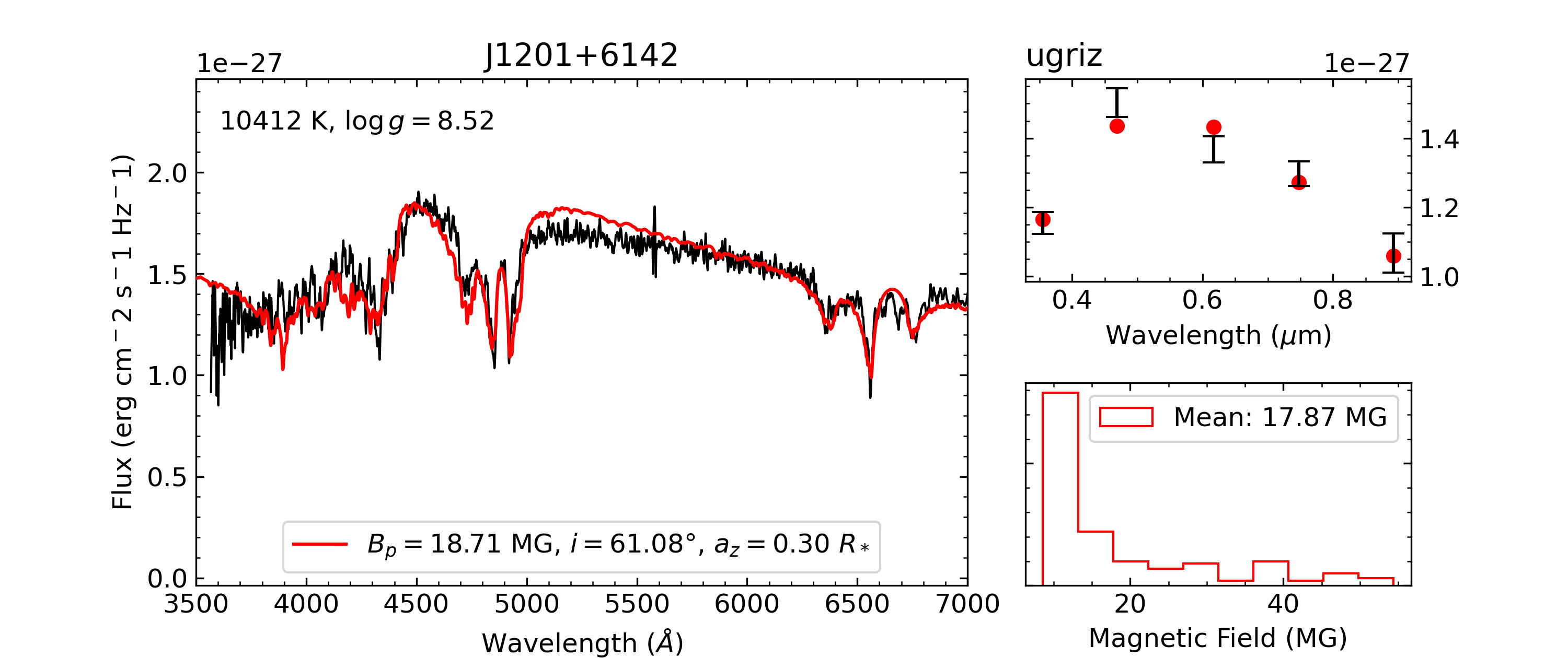
Figure 5: An example of a star that is successfully reproduced by a dipolar field geometry. The left panel is our best fit to the Balmer lines. Upper right panel represents the best fit to the $ugriz$ photometry while the bottom right panel shows the distribution of magnetic field elements at the visible surface of the star for our best fit solution.

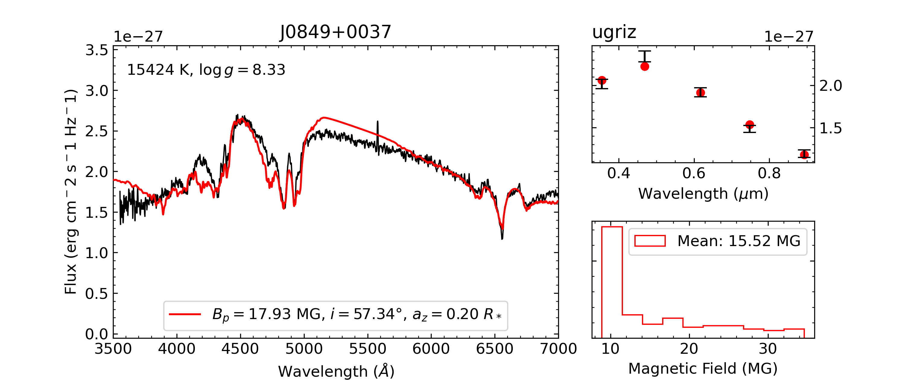
Figure 6: An example for a star where a shifted dipole provides a bad fit.

Another interesting category found within our sample contains objects with hydrogen features that are very shallow compared to what magnetic model spectra predict for the fitted atmospheric parameters and amount of splitting observed (28 objects, Table 3). Figure 7 shows an example of such shallow features. It must be noted that no combination of inclination, offset or field strength can reproduce those spectra. It is also highly unlikely that a more complex multipole expansion could alleviate the issue as the depth of the central component of each line has only a weak dependence on the geometry. In the case of J2257+0755 (EGGR156), Külebi et al. (2009) managed to obtain a good fit by increasing the effective temperature to 40,000 K. This solution, however, is clearly incompatible with the shape of the spectral energy distribution ($ugriz$) which requires an effective temperature in the vicinity of 14,000 K. Lowering the effective temperature below $\sim 10,000$ K also reduces the depth of the absorption features, but again, at the cost of not reproducing the $ugriz$ photometry anymore. Similar objects with shallow features have been modeled has DA+DC unresolved binary in Rolland & Bergeron (2015) but in the case of J2257+0755, the observed photometric modulations rules out a close binary scenario and the star is rather interpreted as the rapidly rotating remnant of a double degenerate merger (Williams et al., 2022). If so, rapid rotation may also produce an unusual surface composition that may explain the shallow lines found in such stars. For example, an attractive solution to the absorption lines depth problem is that such objects have a mixed H-He composition. We experimented with mixed atmosphere and indeed found that it was possible to reduce significantly the depth of the lines in that manner. We calculated models with increasingly more helium, until the depth of hydrogen lines were well reproduced, and found that a 12,000K helium-dominated atmosphere with $\frac{N\left({\rm He}\right)}{N\left({\rm H}\right)}=10^{4}$ can reproduce H$\alpha$ while not predicting helium features that are not observed. Unfortunately, such models badly reproduce H$\beta$. It is possible that the atmosphere is not homogeneous, with patches of different composition and temperature, but exploring the full range of possibilities is beyond the scope of this paper. Again, time-resolved spectroscopy may eventually help us uncover the real nature of such objects. We will thus postpone the analysis of these stars to future studies and exclude them from our discussion below.

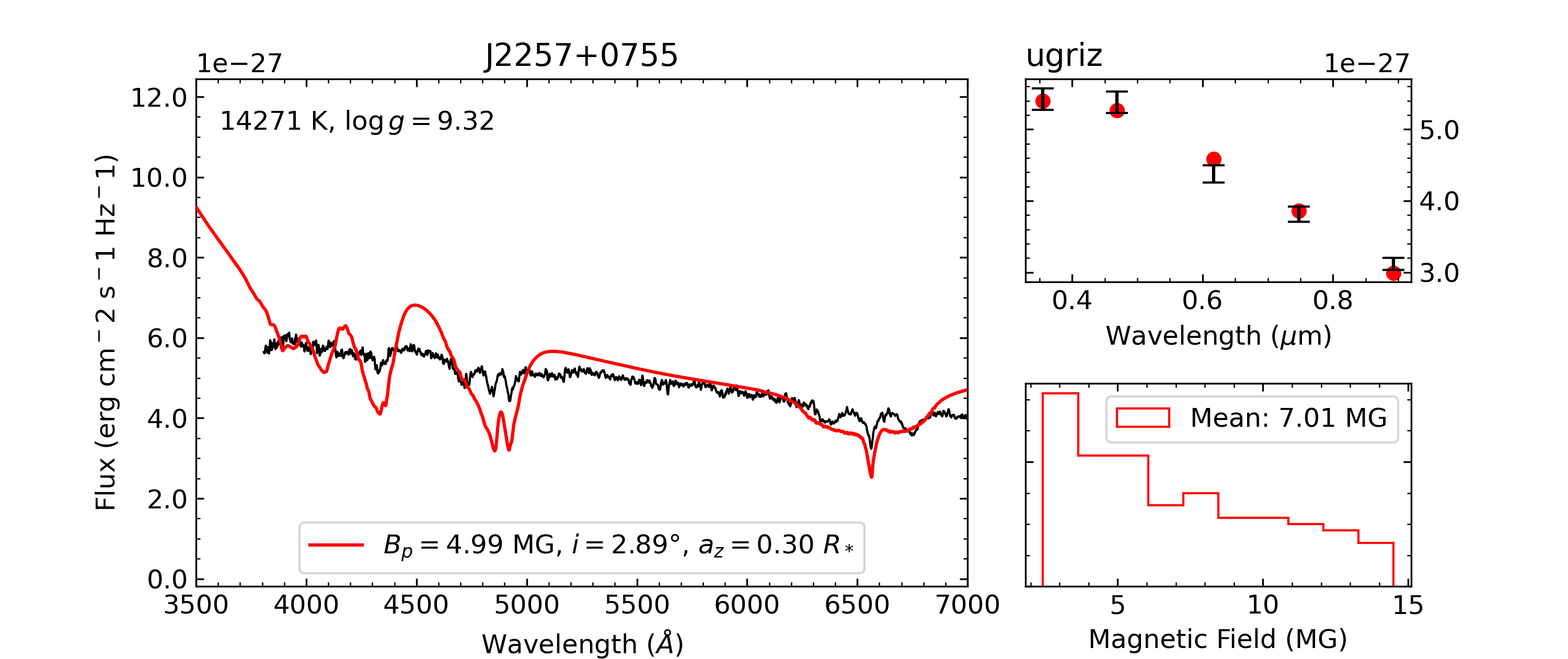
Figure 7: J2257+0755 (EGGR 156), an example of a star whose observed features are too shallow, according to our models. Due to the fitting algorithm trying to minimise the numerical difference between the synthetic spectrum and observations with shallow features, the magnetic structure here is not representative of reality.

Table 3: Stars with shallow features

		J name
J0343$-$0641	J0906+0807	J0944$-$0018	J1057+0411	J1132+2809
J1137+5740	J1201+0847	J1248+4104	J1251+5432	J1314+1732
J1315+0937	J1328+5908	J1332+0117	J1344+3754	J1418+3123
J1430+2811	J1516+2803	J1639+1036	J1816+2454	J2115+0400
J2131+0659	J2138+1123	J2151+5917	J2211+1136	J2223+2319
J2257+0755	J2259$-$0828	J2346$-$1023

Finally, the last category contains stars that could not be fit within our theoretical framework (38, Table 4). These stars are all probably magnetic white dwarfs of some sort since non-magnetic objects at their fitted effective temperature and surface gravity, as obtained from fitting the $ugriz$ photometry, would show strong hydrogen or helium lines that would be easily recognized. An example of such a star is presented in Figure 8 where none of the features could be matched using hydrogen-rich models with offset dipole. The algorithm converged in the parameter space at a place where the surface elements field strength are spread over a large range, effectively washing out spectral features over the entire optical range. While some of the multitude of features produced this way may match those in the observed spectrum, most of it is probably just random coincidences. We thus cannot confirm the hydrogen-rich nature of these stars based on our minimum chi-square solution. It is possible that our failure to find a good solution is due to some large temporal variations of the surface field strength with rotation over timescale much shorter than the integration time of the SDSS spectra. Combined with that, it is also possible the geometry used here (inclined offset dipole) is too simple an assumption and a much more complex geometry is required. Alternatively, the main atmospheric composition of those objects might simply not be hydrogen. In the next paper of that series (Hardy et al. in preparation), we will explore helium-rich compositions and reassess the nature of these objects.

Table 4: Magnetic non DA stars

		J name
J0021+1502	J0211+0031	J0211+2115	J0212+0644	J0333+0007
J0732+1642	J0742+3157	J0800+0655	J0822+1201	J0830+5057
J0836+1548	J0847+4842	J0849+2857	J0856+2534	J0922+0504
J0924+3613	J0935+4429	J1121+1039	J1144+6629	J1153+1331
J1202+4034	J1257+1216	J1308+8502	J1348+1100	J1349+2056
J1407+3011	J1453+0652	J1455+1812	J1532+1647	J1623+3546
J1640+5341	J1704+3213	J1724+3234	J1900+7039	J2151+0031
J2247+1456	J2258+2808	J2346+3853

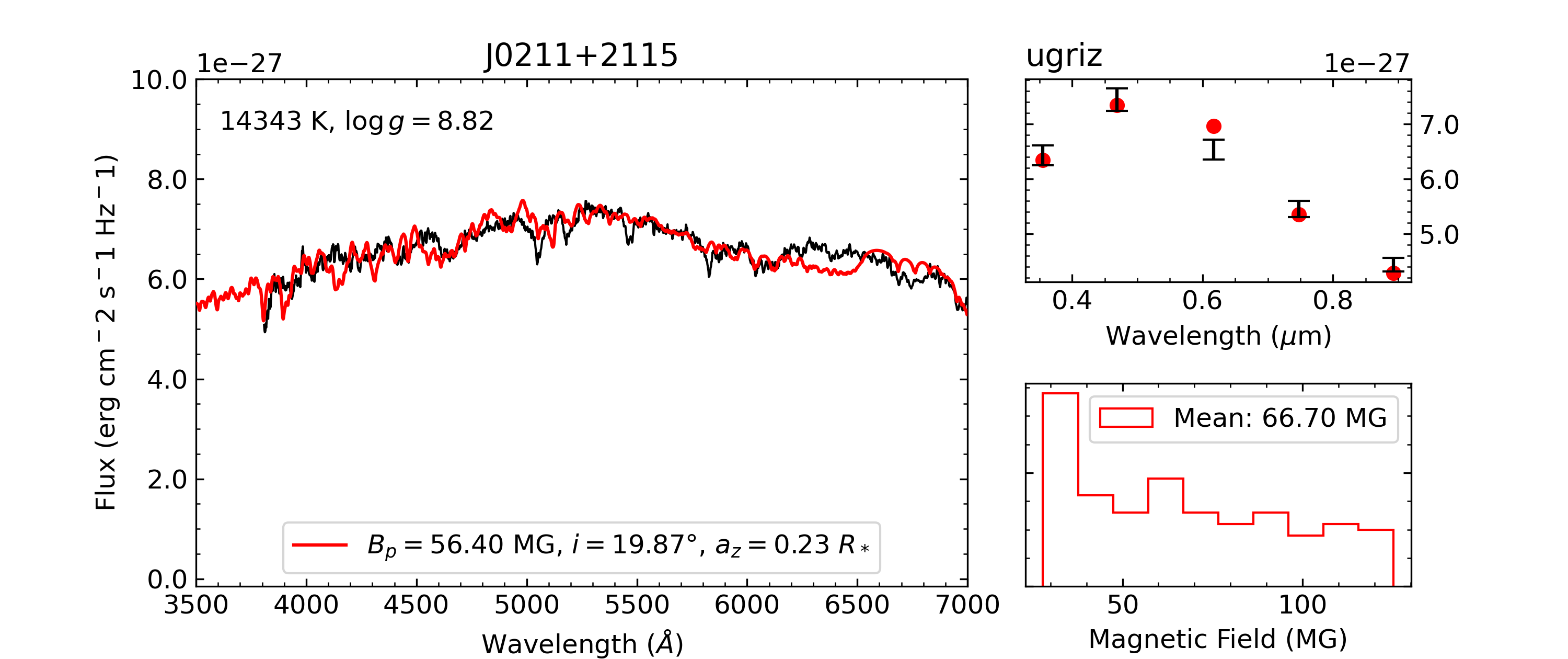
Figure 8: An example of a magnetic white dwarf which we were unable to find a suitable dipolar geometry.

Table 5: Model fits with Good dipole fit

J name	$T_{\rm{eff}}$ (K)	$\log{g}$	Mass ($M_{\odot}$)	$B_{p}$ (MG)	$i$ (deg)	$a_{z}$ ($R_{*}$)	Mean $B$ (MG)
J0010+2451	10760 (603)	8.86 (0.49)	1.129 (0.48)	11.91	55	0.30	12.25
J0014$-$1311	5725 (10)	8.17 (0.0065)	0.696 (0.0086)	18.77	72	0.29	15.46
J0114+1607	20754 (1979)	8.95 (0)	1.178 (0.02)	27.78	84	0.10	18.42
J0257+5103	20595 (655)	8.22 (0.12)	0.753 (0.15)	12.01	56	0.30	12.17
J0318+4226	10465 (174)	8.34 (0.17)	0.817 (0.23)	4.91	24	0.15	4.89
J0326+0521	30000 (0)	8.77 (0.76)	1.099 (0.73)	17.28	63	0.26	15.29
J0419$-$0934	5952 (59)	8.34 (0.044)	0.807 (0.06)	12.81	57	0.29	12.76
J0442+1203	9529 (337)	8.38 (0.068)	0.841 (0.089)	31.69	53	0.28	32.13
J0505$-$1722	5241 (13)	7.83 (0.02)	0.484 (0.022)	7.42	80	$-$0.17	4.53
J0515+2839	6293 (17)	8.17 (0.0085)	0.692 (0.011)	2.22	59	0.30	2.18
J0556+0521	5631 (12)	8.16 (0.35)	0.683 (0.44)	28.99	65	0.29	25.89
J0601+3726	13552 (185)	8.55 (0.023)	0.954 (0.03)	2.30	59	0.30	2.23
J0604+6413	21158 (624)	8.16 (0.12)	0.717 (0.11)	32.08	56	0.24	29.62
J0648+8403	13236 (501)	8.73 (0.88)	1.063 (0.89)	3.70	59	0.30	3.61
J0649+7521	6445 (46)	8.23 (0.035)	0.733 (0.047)	18.24	68	0.30	16.00
J0651+6242	6696 (31)	8.14 (0.028)	0.678 (0.035)	1.22	52	0.30	1.28
J0725+3214	22240 (482)	8.66 (0.23)	1.029 (0.44)	13.83	52	0.06	10.35
J0732+3646	25904 (1239)	9.31 (0.49)	1.306 (0.41)	111.49	63	0.04	78.06
J0736+4033	6320 (30)	8.29 (0.34)	0.773 (0.44)	3.79	70	0.30	3.21
J0742+2328	14852 (573)	8.76 (0.48)	1.079 (0.5)	2.43	58	0.30	2.41
J0748+3025	23078 (1810)	8.38 (0.5)	0.863 (0.58)	8.87	55	0.28	8.81
J0749+1713	21190 (459)	8.07 (0.16)	0.664 (0.12)	13.08	55	0.19	11.37
J0752+1725	9062 (193)	8.41 (0.069)	0.861 (0.091)	12.43	56	0.30	12.52
J0805+2153	30000 (0)	7.55 (0.25)	0.444 (0.15)	3.00	17	0.30	4.08
J0806+0756	15507 (716)	7.45 (0.25)	0.360 (0.14)	2.74	69	0.19	2.13
J0807+3938	15986 (625)	8.16 (0.25)	0.713 (0.33)	37.17	56	$-$0.02	24.92
J0809+3730	15993 (898)	8.51 (0.84)	0.931 (0.87)	51.38	53	0.15	42.99
J0813+2237	22398 (720)	8.42 (0.29)	0.886 (0.36)	13.43	75	0.30	10.68
J0817+2008	6989 (82)	8.30 (0.041)	0.785 (0.054)	3.33	60	0.30	3.22
J0819+3731	11576 (458)	8.32 (0.22)	0.802 (0.28)	10.27	59	0.30	10.03
J0828+2934	23855 (1394)	8.91 (0.14)	1.163 (0.19)	35.30	67	0.23	28.94
J0834+8210	28114 (1103)	9.02 (0.11)	1.211 (0.092)	14.59	66	0.22	11.99
J0839+2000	15392 (363)	8.23 (0.32)	0.755 (0.39)	3.01	67	0.30	2.65
J0840+2712	12768 (593)	8.52 (0.96)	0.935 (0.097)	9.85	64	0.29	8.97
J0841+0223	6769 (57)	8.26 (0.23)	0.756 (0.3)	6.50	51	0.30	6.94
J0842+1539	17263 (296)	7.94 (0.25)	0.582 (0.24)	19.66	76	$-$0.29	11.28
J0845+6117	5625 (31)	8.00 (0.061)	0.587 (0.074)	0.90	23	0.08	0.79
J0851+1201	11074 (315)	8.46 (0.11)	0.893 (0.14)	2.00	78	0.30	1.54
J0851+1527	14323 (854)	8.49 (0.18)	0.916 (0.19)	29.01	67	0.27	24.88
J0855+8249	23693 (511)	8.93 (0.34)	1.173 (0.31)	12.12	68	0.26	10.07
J0908+0921	29293 (1661)	8.93 (0.075)	1.177 (0.072)	51.55	54	0.24	48.85
J0911+4202	11822 (439)	8.66 (0.26)	1.019 (0.31)	50.08	52	0.30	52.92
J0914+0544	17145 (385)	8.45 (0.19)	0.896 (0.24)	9.42	60	0.30	9.12
J0925+0113	9235 (361)	8.26 (0.15)	0.764 (0.19)	2.66	60	0.30	2.58
J0931+3219	13476 (443)	8.23 (0.21)	0.749 (0.21)	9.04	52	0.30	9.49
J0933+1022	7455 (135)	7.46 (0.63)	0.331 (0.044)	2.18	71	0.29	1.83
J0934+2945	20662 (406)	8.23 (0.22)	0.762 (0.23)	26.92	56	0.29	27.01
J0934+3927	9356 (252)	8.19 (0.23)	0.717 (0.28)	2.10	54	0.30	2.18
J0934+5033	8885 (135)	8.35 (0.22)	0.820 (0.28)	9.12	62	0.29	8.50
J0942+2052	21824 (935)	8.78 (0.53)	1.098 (0.53)	40.55	27	$-$0.01	30.22
J0944+4539	16848 (404)	8.57 (0.2)	0.975 (0.3)	16.37	87	0.20	10.92
J0957+1946	14899 (224)	8.70 (0.23)	1.047 (0.45)	4.18	82	0.26	3.00
J1006+3033	10731 (243)	8.14 (0.56)	0.689 (0.65)	4.71	50	0.30	5.10
J1006+4845	9411 (471)	7.76 (0.25)	0.469 (0.2)	8.13	49	0.27	8.44
J1007+1237	18687 (437)	8.04 (0.24)	0.646 (0.24)	6.13	71	0.30	5.15
J1007+1623	11279 (337)	8.73 (0.058)	1.061 (0.068)	13.63	42	0.30	15.89
J1014+3657	10939 (427)	8.26 (0.41)	0.763 (0.51)	14.50	74	0.28	11.47
J1015+0907	7022 (43)	8.27 (0.19)	0.760 (0.25)	4.50	47	0.30	5.00
J1021$-$1034	10485 (124)	8.59 (0.015)	0.979 (0.019)	2.09	59	0.30	2.04
J1022+2725	11581 (606)	8.70 (0.18)	1.045 (0.28)	5.35	51	0.06	4.04
J1025+6229	8578 (311)	8.52 (0.14)	0.928 (0.14)	4.67	57	0.24	4.29
J1029+1127	6691 (72)	8.20 (0.1)	0.716 (0.13)	19.18	46	0.30	21.62
J1034+0327	15756 (406)	8.80 (0.054)	1.104 (0.059)	11.17	77	0.09	7.63
J1054+5933	10704 (383)	8.30 (0.21)	0.788 (0.26)	16.81	63	0.06	11.99
J1056+6523	18833 (616)	8.18 (0.21)	0.731 (0.21)	22.05	44	0.23	22.49
J1103+0534	11233 (369)	8.67 (0.2)	1.029 (0.24)	15.94	68	0.30	13.83
J1110+6001	29215 (361)	8.92 (0.23)	1.171 (0.21)	6.40	70	0.30	5.44
J1118+0952	10438 (325)	8.44 (0.46)	0.881 (0.56)	4.82	63	0.30	4.48
J1120$-$1150	21435 (713)	9.01 (0.62)	1.208 (0.56)	8.57	62	0.30	8.10
J1122+3223	13392 (440)	8.58 (0.12)	0.973 (0.12)	12.22	47	0.30	13.57
J1123+0956	9346 (197)	8.27 (0.034)	0.768 (0.045)	1.85	70	0.30	1.59
J1128+2649	16637 (752)	7.00 (0.25)	0.255 (0.11)	2.34	13	$-$0.12	1.48
J1129+4939	9729 (276)	8.04 (0.085)	0.625 (0.1)	5.49	54	0.30	5.68
J1133+5152	21873 (657)	9.00 (0.042)	1.201 (0.036)	6.06	65	0.30	5.54
J1135+3137	16425 (495)	8.66 (0.18)	1.028 (0.25)	2.99	47	0.19	2.79
J1138$-$0149	12534 (435)	8.28 (0.13)	0.779 (0.17)	25.12	58	0.30	24.75
J1140+6110	15976 (627)	8.11 (0.18)	0.678 (0.14)	66.50	75	$-$0.10	41.20
J1144+1717	19290 (786)	8.35 (0.068)	0.838 (0.088)	2.00	87	0.30	1.38
J1148+4827	28967 (6860)	8.97 (0)	1.194 (0.022)	34.93	65	0.29	31.25
J1152+5018	9231 (476)	8.42 (0.34)	0.869 (0.43)	13.20	50	0.30	14.34
J1154+0117	29316 (325)	8.90 (0.21)	1.162 (0.2)	35.53	87	$-$0.23	22.57
J1159+6139	21591 (887)	8.99 (0.4)	1.197 (0.35)	15.52	50	0.19	14.09
J1201+6142	10412 (482)	8.52 (0.098)	0.936 (0.13)	18.71	61	0.30	17.87
J1205+3408	18753 (424)	8.16 (0.25)	0.714 (0.31)	8.32	48	0.30	9.24
J1210+2214	13177 (426)	8.48 (0.033)	0.908 (0.044)	2.00	86	$-$0.30	1.26
J1217+0828	18583 (282)	8.73 (0.042)	1.066 (0.047)	3.50	74	0.30	2.83
J1222+0015	13888 (953)	9.02 (0.11)	1.206 (0.14)	15.47	83	0.30	11.21
J1222+4811	9350 (218)	8.32 (0.17)	0.804 (0.22)	9.29	66	0.30	8.29
J1223+2307	25989 (312)	8.35 (0.027)	0.848 (0.035)	1.61	24	0.20	1.75
J1224+4155	10054 (364)	8.63 (0.12)	1.004 (0.15)	23.99	75	0.28	19.00
J1227+3855	16592 (621)	8.84 (0.77)	1.123 (0.76)	7.07	68	0.29	6.16
J1227+6612	22843 (586)	8.34 (0.15)	0.832 (0.19)	24.67	43	0.30	28.61
J1234+1248	8246 (68)	7.79 (0.069)	0.479 (0.071)	3.41	47	0.25	3.48
J1248+2942	6611 (44)	7.96 (0.0096)	0.565 (0.011)	3.88	46	0.30	4.38
J1248$-$0229	14263 (459)	8.24 (0.38)	0.756 (0.47)	9.07	71	0.30	7.59
J1250+1549	8614 (535)	7.96 (0.29)	0.576 (0.32)	21.41	62	0.30	20.27
J1254+3710	20315 (412)	8.21 (0.048)	0.748 (0.061)	4.11	57	0.30	4.11
J1254+5612	12870 (448)	8.58 (0.41)	0.973 (0.48)	60.43	62	0.18	49.04
J1257+3414	10148 (245)	8.54 (0.12)	0.948 (0.15)	19.68	72	0.29	16.25
J1300+5904	5976 (53)	7.92 (0.0017)	0.540 (0.0026)	4.79	35	$-$0.01	3.49
J1322+5519	11637 (305)	8.50 (0.25)	0.923 (0.31)	3.85	50	0.30	4.14
J1327+1551	8619 (871)	7.79 (0.25)	0.482 (0.24)	11.19	58	0.24	10.19
J1333+6406	13159 (659)	8.84 (0.081)	1.123 (0.084)	13.37	73	0.28	10.77
J1340+6543	14638 (537)	8.17 (0.24)	0.716 (0.3)	4.82	50	0.30	5.20
J1348+3810	30000 (0)	9.13 (0.034)	1.254 (0.023)	14.66	60	0.22	12.73
J1407+4956	21372 (585)	8.70 (0.76)	1.055 (0.76)	12.68	75	0.19	9.31
J1427+3721	19876 (743)	8.92 (0.037)	1.165 (0.036)	28.48	77	0.13	19.88
J1432+4548	17262 (526)	8.23 (0.23)	0.755 (0.28)	8.19	62	0.29	7.65
J1446+5902	12169 (418)	7.93 (0.25)	0.566 (0.24)	4.00	53	0.24	3.80
J1454+4321	10647 (608)	8.33 (0.028)	0.809 (0.038)	4.07	63	0.30	3.79
J1458+2230	10823 (347)	8.69 (0.3)	1.038 (0.33)	31.69	64	0.28	28.45
J1504+0521	15383 (1011)	8.79 (0.44)	1.101 (0.46)	4.45	54	0.30	4.60
J1508+3945	18708 (388)	7.71 (0.58)	0.473 (0.051)	20.81	56	0.14	16.94
J1514+0744	10572 (727)	8.27 (0.09)	0.770 (0.12)	37.89	53	0.30	39.69
J1514+1520	9252 (293)	8.52 (0.11)	0.931 (0.14)	2.32	53	0.30	2.43
J1515+2445	8718 (187)	8.41 (0.29)	0.862 (0.37)	14.45	62	0.29	13.54
J1524+1856	14611 (553)	8.75 (0.12)	1.077 (0.13)	12.75	61	0.26	11.62
J1538+0842	9656 (221)	8.60 (0.006)	0.983 (0.008)	11.52	49	0.29	12.31
J1538+5306	13965 (451)	8.33 (0.73)	0.818 (0.82)	10.97	36	0.01	8.17
J1542+0348	9835 (318)	8.61 (0.26)	0.987 (0.32)	5.41	34	0.28	6.55
J1543+3432	29554 (563)	8.88 (0.24)	1.151 (0.23)	2.65	60	0.30	2.56
J1548+2451	21161 (344)	8.99 (0.038)	1.198 (0.033)	7.29	73	0.30	6.01
J1647+3709	16762 (296)	8.42 (0.089)	0.878 (0.11)	2.11	52	0.30	2.24
J1650+3411	9797 (299)	8.45 (0.079)	0.884 (0.1)	4.36	55	0.30	4.44
J1652+3334	8965 (178)	8.15 (0.061)	0.687 (0.078)	4.91	49	0.30	5.38
J1652+3528	11615 (501)	8.13 (0.71)	0.683 (0.078)	10.13	62	0.30	9.56
J1659+4401	28957 (811)	9.22 (0.098)	1.283 (0.084)	3.90	50	0.30	4.20
J1707+3532	22872 (502)	8.91 (0.046)	1.161 (0.044)	2.13	62	0.30	2.01
J1714+3918	6577 (26)	7.77 (0.038)	0.461 (0.038)	2.40	50	0.30	2.58
J1717+2620	28729 (1290)	9.15 (0.39)	1.259 (0.31)	21.26	66	0.30	19.14
J1720+5612	24352 (2526)	8.76 (0.15)	1.086 (0.23)	19.03	60	0.10	14.34
J1723+5407	11270 (315)	8.90 (0.049)	1.151 (0.047)	39.18	58	0.09	29.50
J1729+5632	10950 (471)	8.75 (0.12)	1.074 (0.13)	28.57	67	0.22	23.34
J2025+1310	17686 (622)	8.14 (0.12)	0.701 (0.11)	10.62	62	0.30	10.00
J2046$-$0710	8350 (74)	8.25 (0.084)	0.755 (0.11)	2.41	64	0.30	2.22
J2052$-$0016	20823 (428)	8.87 (0.41)	1.143 (0.39)	14.00	78	0.14	9.76
J2149$-$0728	22642 (750)	8.37 (0.14)	0.852 (0.18)	45.09	66	0.17	34.93
J2227+1753	6548 (28)	7.93 (0.006)	0.550 (0.0071)	1.30	40	0.29	1.53
J2332+2658	9497 (197)	8.43 (0.15)	0.870 (0.2)	2.57	57	0.30	2.57
J2348+2535	25122 (396)	8.53 (0.47)	0.959 (0.54)	6.30	44	0.30	7.26

Table 6: Model fits with Bad dipole fit

J name	$T_{\rm{eff}}$ (K)	$\log{g}$	Mass ($M_{\odot}$)	$B_{p}$ (MG)	$i$ (deg)	$a_{z}$ ($R_{*}$)	Mean $B$ (MG)
J0006+0755	8939 (189)	8.26 (0.11)	0.759 (0.14)	13.70	48	0.30	15.05
J0234+2648	15103 (703)	8.39 (0.31)	0.853 (0.39)	45.27	51	0.19	40.78
J0304$-$0025	13190 (533)	8.32 (0.11)	0.807 (0.15)	11.49	59	0.24	10.42
J0331+0045	16796 (268)	8.57 (0.076)	0.974 (0.093)	12.82	58	0.29	12.52
J0345+0034	7345 (77)	7.99 (0.25)	0.589 (0.3)	2.43	45	0.30	2.75
J0537+6759	7661 (45)	8.33 (0.028)	0.804 (0.037)	1.13	61	0.30	1.09
J0632+5559	9876 (37)	8.52 (0.0086)	0.930 (0.011)	0.81	45	0.30	0.92
J0758+3544	22693 (1052)	8.96 (0.12)	1.183 (0.11)	30.90	36	0.30	38.00
J0803+1229	20441 (505)	8.93 (0.0081)	1.172 (0.0081)	37.43	31	0.26	44.25
J0804+1827	11731 (573)	8.66 (0.012)	1.019 (0.016)	72.44	64	0.30	66.52
J0816+0412	12735 (433)	7.84 (0.25)	0.517 (0.22)	10.33	65	0.26	9.02
J0849+0037	15424 (453)	8.33 (0.18)	0.818 (0.22)	17.93	57	0.20	15.52
J0855+1640	16332 (709)	8.43 (0.63)	0.885 (0.72)	15.34	34	0.30	19.11
J0858+4126	7013 (84)	8.37 (0.057)	0.829 (0.076)	2.64	41	0.30	3.09
J0907+3538	18101 (1029)	8.76 (0.14)	1.085 (0.17)	16.44	49	0.26	16.92
J0930$-$0126	14944 (823)	8.91 (0.39)	1.157 (0.37)	21.66	50	0.30	23.41
J0937+1021	19955 (1174)	8.98 (0.64)	1.193 (0.6)	288.08	66	0.14	217.85
J1018+0111	12845 (753)	8.70 (0.14)	1.045 (0.16)	76.07	16	0.05	64.24
J1018+3033	21298 (437)	8.78 (0.15)	1.098 (0.19)	50.92	78	0.24	37.68
J1020+3626	19101 (1071)	8.31 (0.18)	0.813 (0.23)	59.79	69	0.15	44.69
J1022+1949	8673 (189)	8.38 (0.33)	0.838 (0.42)	2.65	30	0.30	3.37
J1033+2309	26025 (1171)	8.77 (0.15)	1.097 (0.15)	230.49	40	0.26	254.52
J1035+2126	6882 (53)	8.09 (0.021)	0.644 (0.027)	2.63	48	0.30	2.89
J1126+0906	11623 (496)	8.86 (0.04)	1.132 (0.04)	26.08	2	0.28	35.13
J1130+3057	10767 (384)	8.55 (0.18)	0.952 (0.22)	3.94	30	0.29	4.96
J1206+0813	15163 (998)	8.80 (0.26)	1.103 (0.27)	180.54	50	0.30	194.44
J1216$-$0026	16409 (1263)	8.83 (0.18)	1.118 (0.27)	63.24	53	0.27	63.85
J1242+4548	11667 (393)	8.56 (0.22)	0.963 (0.39)	10.93	21	0.30	14.57
J1351+5419	13937 (1038)	8.43 (0.27)	0.882 (0.34)	368.52	34	0.07	303.55
J1508+2150	19995 (406)	8.17 (0.12)	0.726 (0.15)	23.78	42	0.30	27.78
J1511+4220	11595 (411)	8.72 (0.09)	1.054 (0.11)	14.01	40	0.30	16.61
J1517+6105	10751 (782)	8.83 (0.12)	1.118 (0.14)	10.27	47	0.11	8.45
J1535+4213	18696 (2151)	7.70 (0.25)	0.469 (0.18)	5.99	83	$-$0.29	3.65
J1557+0411	24847 (1220)	9.04 (0.044)	1.218 (0.037)	43.83	55	0.25	41.65
J1601+0442	20251 (983)	8.52 (0.44)	0.942 (0.52)	92.59	18	0.03	75.75
J1603+1409	10547 (348)	8.62 (0.017)	0.996 (0.022)	48.88	47	0.23	48.74
J1604+4908	10717 (478)	8.67 (0.15)	1.023 (0.18)	67.10	40	0.30	80.07
J1608+0644	9407 (256)	8.51 (0.41)	0.925 (0.5)	22.71	37	0.30	27.63
J1633+1942	16393 (230)	8.13 (0.045)	0.695 (0.056)	3.61	54	0.30	3.72
J1648+4618	14608 (473)	8.31 (0.11)	0.803 (0.14)	19.48	50	0.30	21.18
J1709+2341	13784 (817)	8.53 (0.19)	0.943 (0.26)	12.07	50	0.28	12.72
J2117$-$0736	26033 (1002)	9.02 (0.12)	1.211 (0.15)	6.24	51	0.30	6.71
J2149+0048	14121 (484)	8.67 (0.17)	1.032 (0.23)	9.57	54	0.27	9.55
J2218$-$0000	16678 (702)	8.84 (0.12)	1.127 (0.12)	96.00	20	0.28	123.63
J2322+0039	20241 (573)	8.97 (0.58)	1.188 (0.52)	11.00	19	0.10	10.12

5 Discussion

From our original sample, we are left with 185 objects that we could fit with various degrees of quality using a dipolar geometry. Figure 9 shows that including the effect of the magnetic field in the synthetic color calculations tends to systematically increase the determined effective temperature compared to that obtained from non-magnetic models (the difference can be as high as 3700K for stars with the largest field intensity). As explained in Section 3.2, this is a direct consequence of the shifting of absorption lines across adjacent photometric bands as the magnetic field strength increases. To compensate for this increase in effective temperature, it becomes necessary to decrease the stellar radii in order to reproduce the photometric data. Hence, the derived masses are also increased by up to $0.1\,M_{\odot}$ compared to masses determined from non-magnetic models (see Figure 10).

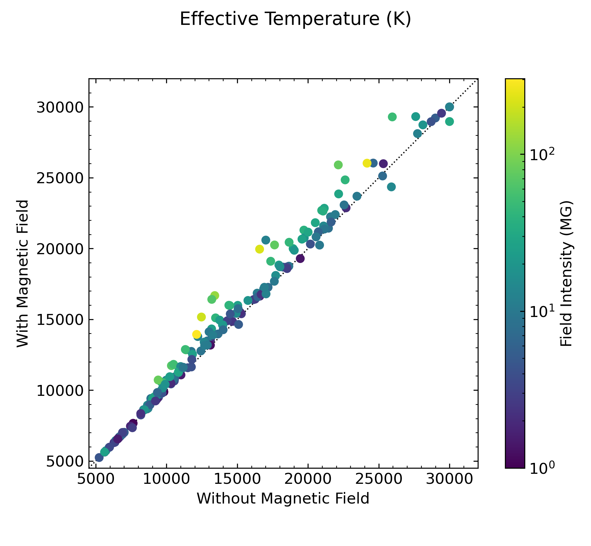
Figure 9: Comparison of effective temperatures obtained from non-magnetic vs. magnetic synthetic spectra. The color scale indicate the strength of the magnetic field.

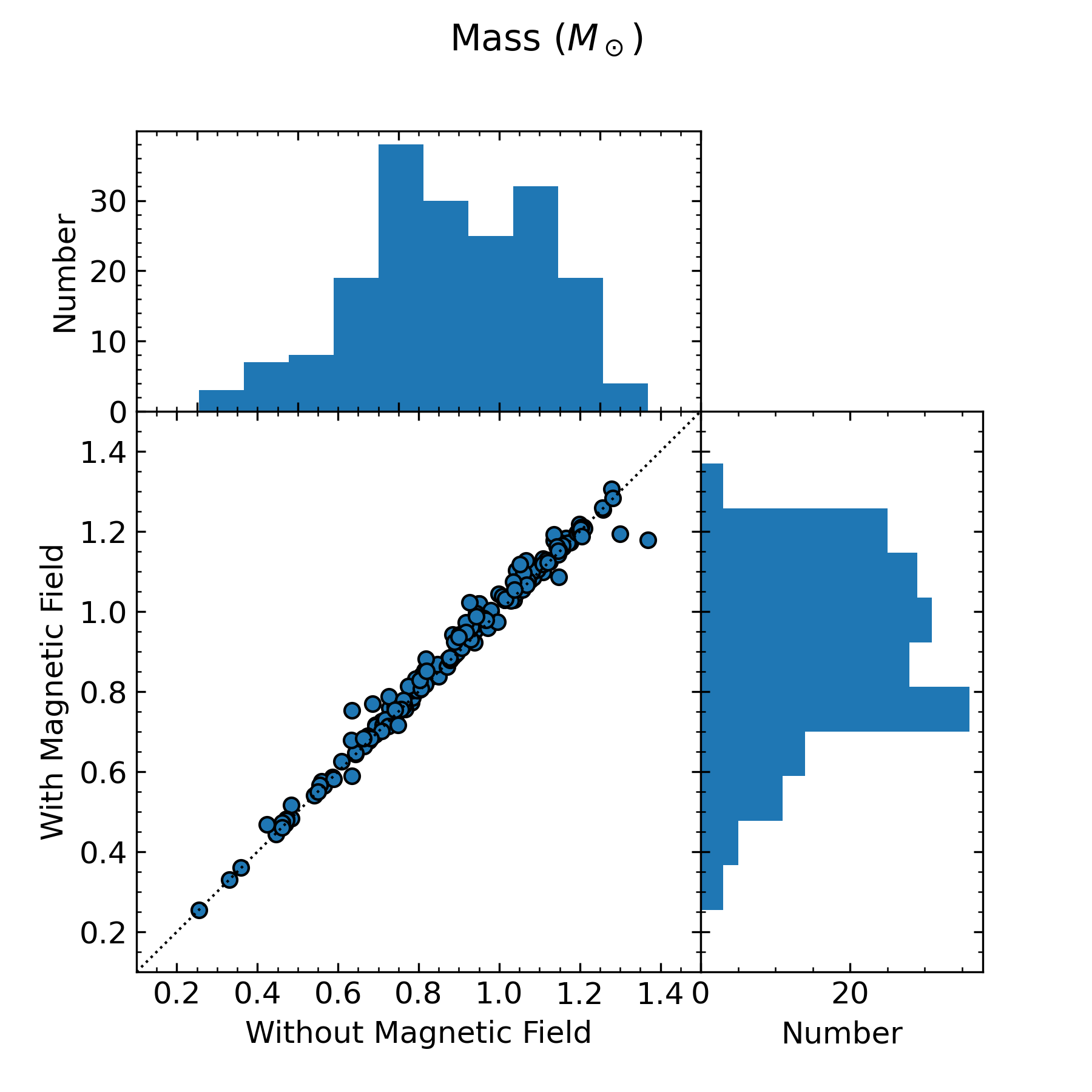
Figure 10: Comparison of stellar masses obtained from non-magnetic vs. magnetic synthetic spectra. The corresponding mass distribution histograms are also shown on the right and upper part of the figure.

It is interesting to discuss our sample in light of the results drawn from the 40 pc sample recently presented by Bagnulo & Landstreet (2022). According to their interpretation, MWDs form two distinct populations distinguished by their very different typical masses. The most massive magnetic white dwarfs, according to their hypothesis, would mostly be the result of binary mergers, producing strong magnetic fields that would be present at the surface as soon as the star enters the cooling sequence. Such mergers are expected to be rapidly rotating. On the other hand, young MWDs with mass below about $\sim$ $0.75\,M_{\odot}$ appear to be extremely rare and magnetism would gradually appear only after 2 Gyr or 3 Gyr, possibly due to the relaxation of a preexisting field buried in the interior or generated by a dynamo mechanism triggered by the onset of core crystallization (Isern et al., 2017; Schreiber et al., 2021).

Figure 11 takes a closer look at the mass distribution of our sample as well as all the stars that we rejected in the previous section. First, we see that the stars previously classified DAH that we dismissed as magnetic form a relatively broad distribution centered on $\sim$$0.6\,M_{\odot}$, as expected for a population of non-magnetic white dwarfs. This unusually large distribution can easily be explained by the fact that those stars are almost twice as distant, on average, than the stars that we successfully fit with a dipole. These were thus objects with the very lowest signal-to-noise ratio spectra of the sample, and the observed splitting that led to their classification as DAH was most probably just noise. Being more distant, the uncertainties on the photometric data and parallax measurements were also much larger, explaining the extremely broad mass distribution.

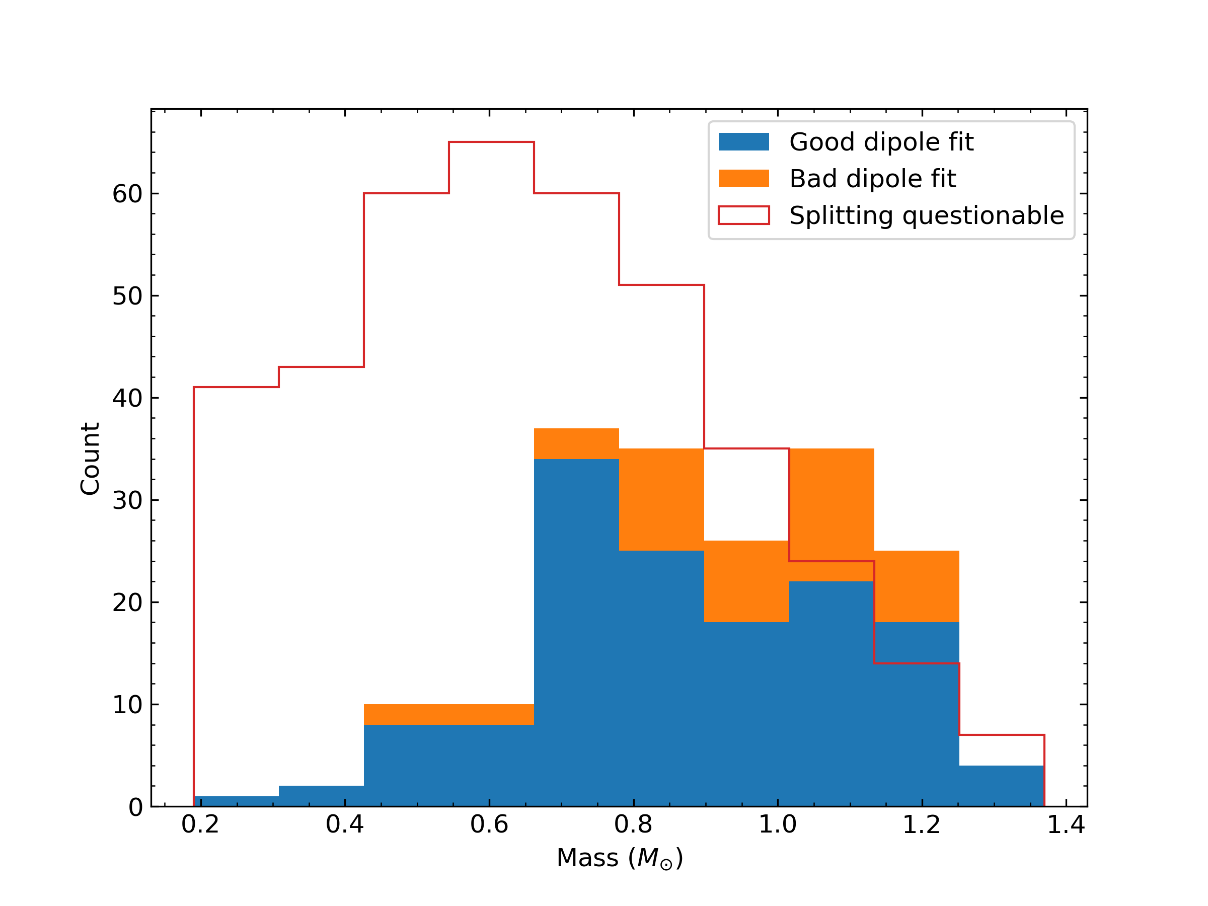
Figure 11: Mass distribution for the stars in our sample.

Next, we observe a sudden increase in the number of MWDs at a mass of about $0.7\,M_{\odot}$. This may indicate that the most massive MWDs have a different origin than the ones at lower mass, as suggested by Bagnulo & Landstreet (2022). We must, however, remain cautious with this interpretation as our sample is mostly drawn from a magnitude-limited survey that certainly suffer from a number of selection biases difficult to quantify. Nevertheless, a look at the distance distribution of our sample in Figure 12 suggests that the preponderance of massive white dwarfs in our magnetic sample is real and not merely an artifact of various selection effects. Indeed, while it can be argued that massive white dwarfs may be, due to their much smaller radii, underrepresented in a magnitude limited sample, the fact that we see a cutoff in the number of magnetic stars with mass above $0.75\,M_{\odot}$ starting at about 250 pc suggest that we are perfectly capable of identifying such objects in SDSS at smaller distances. Meanwhile, MWDs less massive than $0.75\,M_{\odot}$ are much larger (and thus brighter) and would be, at similar effective temperature, easily identify in that same volume, assuming that whatever selection bias affecting our sample is the same at all white dwarf masses. According to the reasoning of Bagnulo & Landstreet (2022) described above, this is totally to be expected if magnetism in lower mass objects only appears much later on the cooling sequence. The big difference with our sample is that contrary to what is observed in the 40 pc sample, low mass MWDs are not completely absent for ages younger than 1-2 Gyr (see Figure 13). Taking only objects within 250 pc does not change the overall picture emerging from Figure 13 much; young MWDs less massive than $0.75\,M_{\odot}$, while much rarer than heavier ones, do exist. Their magnetic field strength, however, never reach values above $\sim$30 MG as is regularly found at higher masses. It is possible, however, that whatever mechanism is responsible for the presence of strong magnetic fields in young low mass white dwarfs is sufficiently rare for it to not be statistically present in the 40 pc sample and that only looking at a much larger volume does this additional channel manifest its presence. To summarize, our sample does suggest white dwarfs with strong magnetic field and mass above $0.75\,M_{\odot}$ are much more numerous than their lower-mass counterpart. While selection biases may play a role in the exact proportion, this assessment is unlikely to change with a large volume-limited sample. The young low mass MWDs in our sample could represent a separate channel not observed in the 40 pc sample that is superposed to the one where magnetism only start to show up after the onset of crystallization in the core.

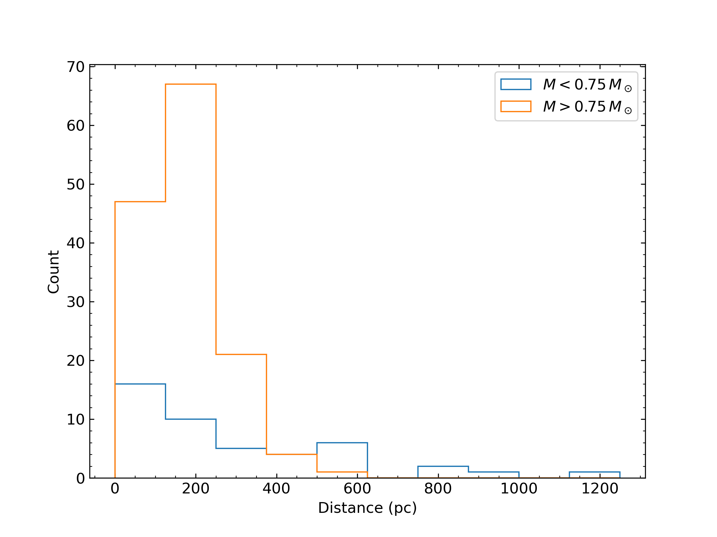
Figure 12: Distance distribution of confirmed Magnetic DA stars, divided into two groups: One with masses below $0.75\,M_{\odot}$, the other with masses above.

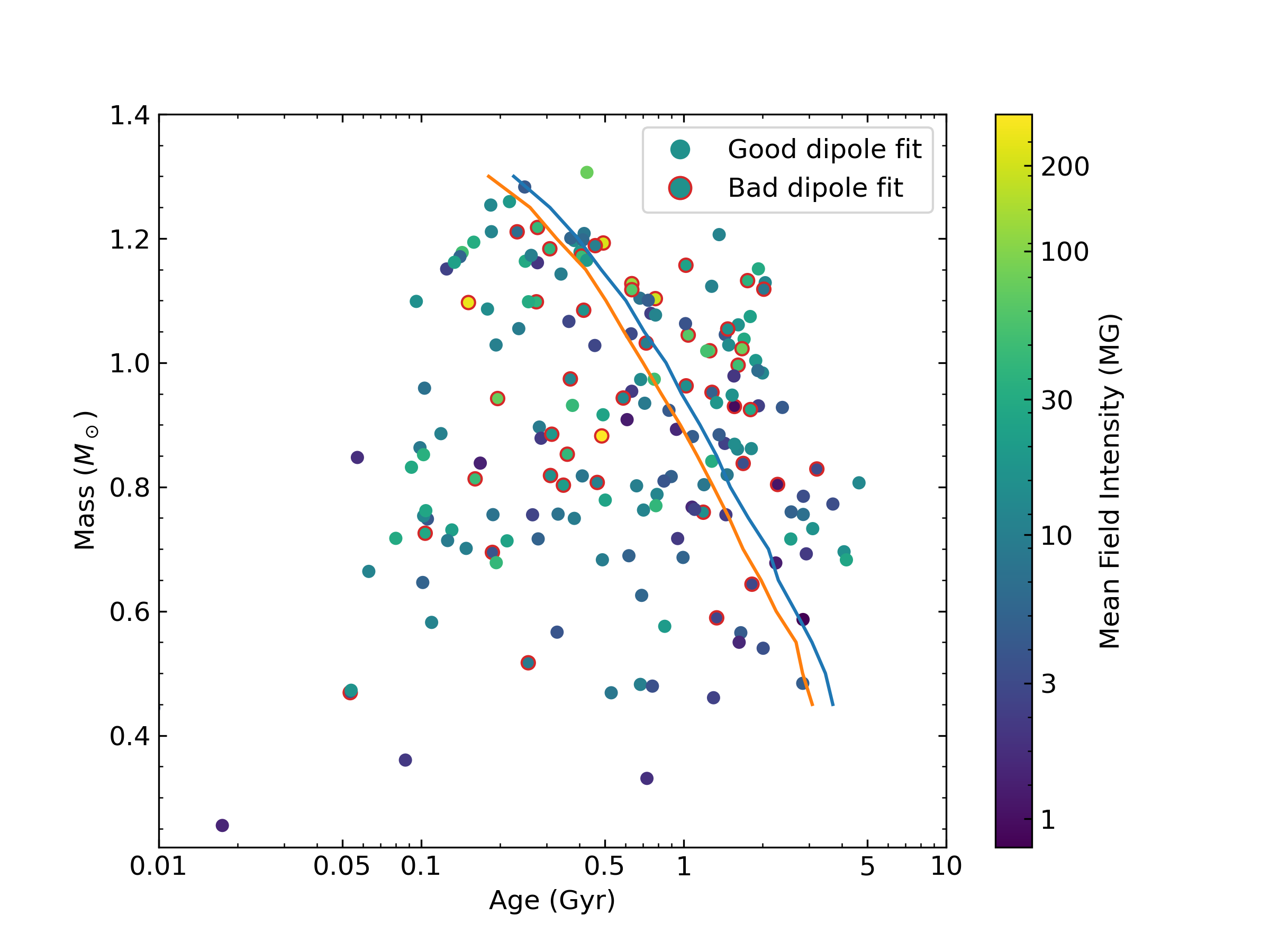
Figure 13: Stellar mass vs. age, color coded with the mean surface magnetic field for the confirmed stars in our sample. The blue and orange lines represent the onset of crystallization for stars with a thick ($q_{He}=10^{-2}$, $q_{H}=10^{-4}$) and thin ($q_{He}=10^{-2}$, $q_{H}=10^{-10}$) hydrogen layer, respectively.

Are there other signatures for different channels/origin that emerge from the homogeneous analysis of the sample? Figure 14 shows little correlation between the mean dipole field intensity (mean field intensity on the visible surface of the star) and stellar mass, except for the fact that all the largest fields are found only in high mass white dwarfs. The stars that were badly fit with a dipole are slightly more prevalent among the most massive ($M\geq$ $0.75\,M_{\odot}$) and most magnetic ($B\geq$ 10 MG) but can nevertheless be found at any mass, field or effective temperature. We can see a slight tendency for heavier stars to be hotter, as there is a higher density of $>25000$ K stars near $1.2\,M_{\odot}$, although this could be a selection bias since more massive stars are smaller, and need to be hotter and more luminous to be seen at a given magnitude. Looking instead at the effective temperature vs. the mean dipole field intensity (Figure 15) does not highlight any discernable pattern that would allow us to distinguish between different groups that would possibly have different origins. Such distinction may require a detailed analysis based on time-resolved spectroscopy in order to pinpoint possible differences in field structures.

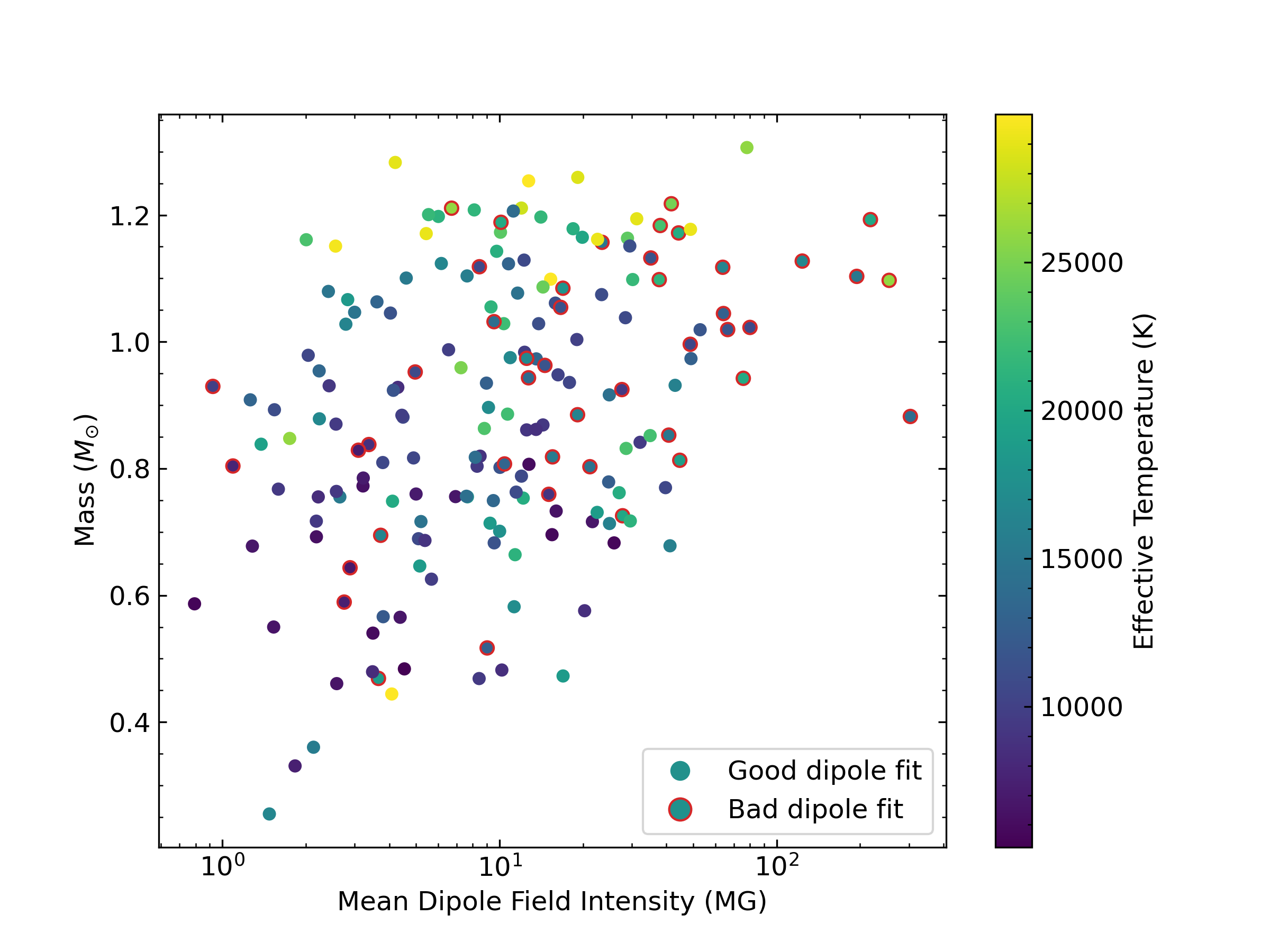
Figure 14: Mass vs. magnetic field intensity for the confirmed magnetic stars in our sample. The color scale shows effective temperature for each star.

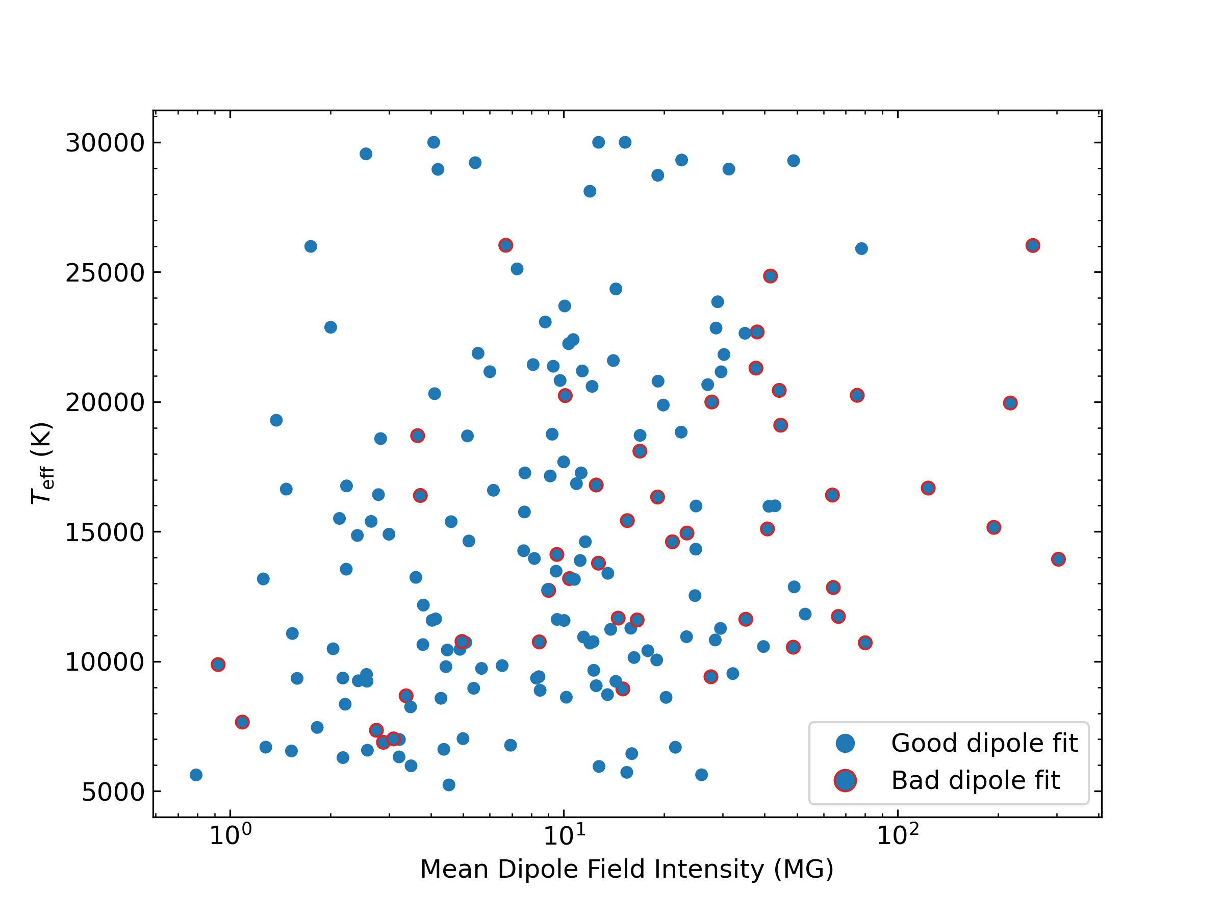
Figure 15: Effective temperature vs. magnetic field intensity for the confirmed magnetic stars in our sample.

6 Conclusion

In this study, we used state-of-the-art magnetic synthetic models to perform the first large homogeneous analysis of hydrogen-rich MWDs since 2009. We carefully examined 651 white dwarfs that were labeled as magnetic or DAH compiled in the Montreal White Dwarf Database. Since most of the sample is drawn from the Sloan Digital Sky Survey, only white dwarfs with magnetic fields large enough to produce an undeniable line splitting (above $\sim$1-2 MG) could be assessed. From our original sample, 400 stars are reclassified as non-magnetic white dwarfs as the alleged splitting reported in the literature did not hold up against attentive scrutiny. We find that 140 stars could be relatively well fitted with an offset dipole while another 45 were clearly DAH but a dipolar fit was passable. We were also unable to fit 38 objects with our theoretical framework, suggesting that these objects either have a much more complex field structure or are simply not hydrogen-rich. Finally, the depth of the absorption line for 28 stars were too shallow compared to model predictions, possibly due to non-homogeneous/mixed surface compositions.

We find a sharp increase in the number of MWDs starting at a mass of about $0.70\,M_{\odot}$. The strongest magnetic fields are also found only among the most massive white dwarfs (no field above 30 MG are found for $M\leq$ $0.70\,M_{\odot}$). Stars that are well and badly fitted with a dipole geometry appear to be disseminated evenly across the whole range of masses, effective temperatures and magnetic field strengths, leaving little clues about their possibly different origins. The stars badly fitted with a dipole could have a much more complex field structure or simply vary on short time scaled compared to the spectra integration time. Signature of the evolutionary origin of the magnetic field, if present, will have to wait for the availability of time-resolved spectroscopy in order to better quantify the details of their field structure.

A study of the 40 pc sample by Bagnulo & Landstreet (2022) recently suggested that magnetism in white dwarf star with masses below $0.75\,M_{\odot}$ only start to appear after about 2 Gyr, possibly as the result of a dynamo mechanism that is triggered by the start of core crystallization. However, based on our sample, it appears that there is an additional channel that is capable of producing very young magnetic white dwarfs with $M\leq$ $0.70\,M_{\odot}$. With about two dozen such object found in a volume much larger than the 40 pc sample, it may, however, not be statistically significant to not find any in the local sample. Because our sample certainly suffer from numerous selection biases, we refrain from quantifying the proportion of such objects as a function of age or mass.

To conclude, detailed analysis of large samples of magnetic white dwarfs are needed to provide new insights on the nature and evolution of such stars. Our study, while inconclusive, represent the largest effort in that endeavor since the work of Külebi et al. (2009), almost doubling the number of magnetic white dwarfs meticulously analyzed in a homogeneous fashion. Our investigation established the existence of various families of magnetic objects that deserve further scrutiny, especially those not fit well with a dipole geometry or those with shallow absorption features. Some object that may not have a hydrogen-rich surface composition will be examined in detail in the next paper of this series. Time-resolved spectroscopy, spectropolarimetry and much higher signal-to-noise/resolution observations are highly awaited for advancing our understanding of the origin and evolution of magnetic white dwarfs. The unique models and fitting tool developed for this project have certainly proven themselves as reliable, and will be the basis of studies that will push even further our understanding of MWDs.

Data Availability

The data underlying this article are available on the Montreal White Dwarf Database (Dufour et al., 2017).

Table 7: Object Names and Coordinates

J Name	Gaia Source ID	MWDD ID	R.A.	Decl.
J0002$-$4310	4994877094997259264	LAWD 96	0.54831	$-$43.16834
J0003$-$0153	2448780654695945728	SDSS J000321.59$-$015310.8	0.84005	$-$1.88640
J0005+1934	2798285095877328512	SDSS J000528.70+193457.4	1.36971	19.58270
J0006+0755	2746037712074342784	SDSS J000603.80+075514.4	1.51576	7.92059
J0007+2407	2849716401534278784	SDSS J000701.59+240744.7	1.75682	24.12903
J0010+2429	2849087274724833408	SDSS J001050.27+242946.6	2.70947	24.49616
J0010+2451	2850233721754720896	SDSS J001034.95+245131.2	2.64549	24.85856
J0012+5025	395234439752169344	GJ 1004	3.05832	50.42005
J0014$-$1311	2418116963320446720	GJ 3016	3.55088	$-$13.18671
J0016+2350	2849169050901523072	SDSS J001616.50+235040.2	4.06876	23.84449
J0021+1502	2792315366213367296	SDSS J002128.59+150223.8	5.36923	15.03963
J0040+0702	2557135773267479424	SDSS J004011.49+070255.7	10.04790	7.04880
J0040+2438	2806537411679838976	SDSS J004038.90+243852.8	10.16214	24.64798
J0042+2358	2803444588550040448	SDSS J004254.24+235831.3	10.72608	23.97536
J0054+1202	2774977549607430528	PHL 886	13.57627	12.03342
J0101$-$0411	2525337076653338240	GD 9	15.25968	$-$4.18613
J0103+1511	2777517245373757824	SDSS J010311.34+151110.0	15.79729	15.18614
J0104+1459	2777498553676004736	SDSS J010405.12+145907.2	16.02132	14.98505
J0109+1800	2785085218267094784	SDSS J010952.81+180000.5	17.47006	18.00003
J0111+1410	2590989117810901120	[BGK2006] J011130.67+141049.7	17.87779	14.18040
J0112+2653	306921489708694912	SDSS J011256.83+265313.4	18.23686	26.88704
J0114+1607	2783824250228883456	SDSS J011423.35+160727.5	18.59728	16.12428
J0117+2422	294036523396554112	SDSS J011739.82+242236.3	19.41600	24.37671
J0117+3035	310263592740515584	SDSS J011708.71+303547.7	19.28629	30.59653
J0121+3210	316660791909483904	SDSS J012115.45+321010.0	20.31439	32.16953
J0121+3932	371598302707808000	SDSS J012105.53+393239.6	20.27306	39.54434
J0122+0827	2578511413182367744	SDSS J012215.76+082712.8	20.56582	8.45352
J0125$-$1013	2470843455019468416	SDSS J012516.70$-$101313.9	21.31962	$-$10.22053
J0126+1934	2786290283011651712	SDSS J012646.78+193454.5	21.69502	19.58180
J0137+2351	291652468654641024	SDSS J013742.54+235138.3	24.42726	23.86059
J0138+2523	292454841560140032	PG 0136+251	24.72099	25.38940
J0143+1437	2588273117931959168	SDSS J014354.00+143746.0	25.97502	14.62950
J0143$-$1015	2463936769649897472	SDSS J014307.12$-$101523.8	25.77974	$-$10.25642
J0148$-$0048	2509104161858231552	SDSS J014823.30$-$004807.5	27.09714	$-$0.80210
J0203+2205	97582241081363712	SDSS J020316.65+220527.2	30.81949	22.09081
J0205+0030	2507984652863078400	SDSS J020514.53+003100.3	31.31064	0.51661
J0207+2238	100719903669705600	SDSS J020700.16+223848.9	31.75077	22.64694
J0211+0031	2507283744264600192	WD 0208+002	32.81856	0.52445
J0211+0722	2521131650835365120	SDSS J021107.71+072235.4	32.78221	7.37649
J0211+2115	99498964725981440	2MASS J02114816+2115491	32.95130	21.26328
J0212+0644	2521035817229538688	PB 6737	33.02212	6.73910
J0213+0530	2519862844481638528	SDSS J021338.52+053023.4	33.41051	5.50624
J0218+0355	2514958747743590144	SDSS J021818.18+035525.3	34.57573	3.92368
J0230+2508	102390302349905024	SDSS J023035.63+250831.6	37.64871	25.14191
J0231+2648	127338977098826496	SDSS J023157.00+264837.5	37.98756	26.81034
J0234+2648	127373577355161984	SDSS J023420.62+264801.6	38.58594	26.80045
J0235+2416	102046155210274560	SDSS J023542.73+241653.8	38.92807	24.28155
J0242+2916	129560166680749952	SDSS J024241.67+291608.3	40.67367	29.26896
J0249+3327	139669072291373696	SDSS J024903.02+332737.1	42.26256	33.46026
J0250+3414	139837366290146432	SDSS J025016.66+341426.8	42.56943	34.24075
J0257+5103	440396914222763264	KPD 0253+5052	44.34168	51.06214
J0259+0811	8578256576520320	EGGR 476	44.99853	8.19868
J0301+0539	6872772307840512	SDSS J030107.57+053957.0	45.28151	5.66577
J0304$-$0025	3266337781252698880	WD 0301$-$006	46.03077	$-$0.42834
J0305+0502	3819840833880704	SDSS J030522.15+050213.3	46.34230	5.03698
J0305+3707	139423576256627584	SDSS J030550.35+370759.2	46.45977	37.13313
J0307+3628	138958134945485184	SDSS J030725.78+362825.9	46.85746	36.47377
J0310+0451	3942127143088128	SDSS J031058.73+045130.1	47.74478	4.85839
J0318+4226	239717998989931136	SDSS J031824.20+422650.9	49.60098	42.44741
J0319+4103	239300974845345664	SDSS J031929.02+410316.9	49.87091	41.05463
J0326+0403	3275317320918274944	SDSS J032658.76+040308.2	51.74498	4.05196
J0326+0521	3275755819899175936	SDSS J032628.17+052136.3	51.61741	5.36004
J0331+0045	3264649412428917376	WD 0329+005	52.94050	0.75470
J0333+0007	3264551560189562112	WD 0330$-$000	53.33525	0.12237
J0340$-$0635	3244183790184727936	SDSS J034046.43$-$063528.0	55.19346	$-$6.59107
J0343$-$0044	3251533926632805120	SDSS J034323.25$-$004410.2	55.84688	$-$0.73619
J0343$-$0641	3244357341222727168	WD 0340$-$068	55.78407	$-$6.69099
J0344$-$0514	3244790651883847168	SDSS J034420.66$-$051444.6	56.08608	$-$5.24570
J0345+0034	3269671637947408128	WD 0342+004	56.29607	0.57883
J0346+0948	3302650084770597760	SDSS J034630.98+094827.5	56.62931	9.80745
J0347+1000	3302679909023476096	SDSS J034748.58+100048.6	56.95243	10.01344
J0350+0858	3302347027581060864	SDSS J035010.32+085829.2	57.54303	8.97476
J0357$-$0439	3245786671979697024	SDSS J035738.13$-$043954.4	59.40904	$-$4.66513
J0419$-$0934	3191738120628213760	LP 714$-$52	64.83730	$-$9.57521
J0442+1203	3295875993630625664	SDSS J044254.59+120329.9	70.72746	12.05826
J0443+1131	3294294788534366336	SDSS J044329.34+113154.8	70.87225	11.53186
J0445$-$0525	3200460782593500160	SDSS J044512.39$-$052524.5	71.30164	$-$5.42351
J0446+1015	3293223142655086720	SDSS J044641.49+101511.0	71.67288	10.25297
J0452+2519	153229044254825728	GALEX J045219.3+251935	73.08070	25.32564
J0505$-$1722	2982808337003815040	GJ 3329	76.46935	$-$17.37589
J0515+2839	3422405214775411840	2MASS J05155350+2839169	78.97394	28.65423
J0534+6254	286502978963267968	SDSS J053400.84+625419.8	83.50353	62.90554
J0535+0016	3220896408787293824	SDSS J053507.04+001617.2	83.77934	0.27139
J0537+6759	481698110012697728	Gaia DR2 481698110012697728	84.31182	67.99710
J0556+0521	3320184202856027776	V* V1201 Ori	89.10610	5.36342
J0601+3726	3456777730670779776	PM J06019+3726	90.49468	37.43346
J0604+6413	1008208457083941888	SDSS J060442.49+641357.1	91.17706	64.23248
J0632+5559	995112350178946048	Gaia DR2 995112350178946048	98.14944	55.98380
J0641+4744	966561537900256512	GD 77	100.30332	47.73806
J0645+2803	3386204893943003136	SDSS J064532.74+280330.5	101.38642	28.05843
J0648+8403	1149683305424619520	SDSS J064828.76+840340.9	102.11972	84.06126
J0649+7521	1115546944012493696	Gaia DR2 1115546944012493696	102.36220	75.35688
J0651+6242	1100089318058003328	PM J06513+6242	102.84537	62.71456
J0714+4012	948379837528696320	SDSS J071410.26+401219.5	108.54277	40.20538
J0716+3935	948104306786401664	SDSS J071632.91+393553.7	109.13716	39.59825
J0725+3214	892902226002248448	SDSS J072540.82+321402.1	111.42009	32.23389
J0727+4036	900558331625377024	SDSS J072724.66+403622.0	111.85282	40.60580
J0730+3627	898573713137494784	SDSS J073001.65+362713.1	112.50692	36.45357
J0731+3531	895445980512796416	SDSS J073135.37+353108.6	112.89738	35.51902
J0732+1642	3169153597742027520	SDSS J073249.55+164205.5	113.20644	16.70154
J0732+3646	898629307193262976	SDSS J073237.68+364628.9	113.15697	36.77457
J0733+6409	1089400763661597440	GJ 1098	113.37909	64.15651
J0735+6526	1089770092196067712	SDSS J073546.51+652656.0	113.94378	65.44883
J0736+4033	924374548053164800	SDSS J073615.93+403335.2	114.06623	40.55966
J0738+2236	867032401028023680	SDSS J073858.45+223608.3	114.74361	22.60231
J0742+2328	867185649757179520	SDSS J074224.66+232804.1	115.60267	23.46777
J0742+3157	880354496226790400	SDSS J074213.37+315703.2	115.55557	31.95081
J0746+1538	3164903950940416000	SDSS J074640.54+153831.8	116.66890	15.64218
J0746+2818	875378381478425472	SDSS J074651.79+281817.2	116.71585	28.30478
J0748+3025	879036662822100224	SDSS J074853.07+302543.5	117.22111	30.42870
J0749+1545	666900157830877312	SDSS J074907.49+154534.0	117.28118	15.75948
J0749+1713	667924932731149312	SDSS J074924.91+171355.3	117.35379	17.23202
J0750+2220	674672635590813568	SDSS J075036.55+222021.5	117.65227	22.33930
J0752+1725	668251556403678592	SDSS J075234.95+172524.9	118.14549	17.42348
J0752+2831	875526407526791552	SDSS J075245.77+283141.2	118.19073	28.52809
J0756+1427	654484193355487872	SDSS J075604.59+142746.0	119.01909	14.46278
J0757+0855	3146973802509252352	SDSS J075704.00+085520.1	119.26666	8.92222
J0758+1214	3151260351669028992	SDSS J075816.64+121428.7	119.56930	12.24124
J0758+1439	654573837912653312	SDSS J075813.39+143902.7	119.55574	14.65075
J0758+3544	906772187229375104	SDSS J075819.57+354443.7	119.58130	35.74525
J0800+0655	3144237908341731712	SDSS J080042.47+065542.1	120.17677	6.92838
J0800+8327	1149262467348564736	SDSS J080014.57+832724.7	120.06096	83.45689
J0801+0643	3144219182284172928	SDSS J080132.78+064349.7	120.38655	6.73047
J0802+1530	655029070086144000	SDSS J080210.39+153033.8	120.54322	15.50940
J0803+1229	653051877600013312	SDSS J080359.93+122943.9	120.99977	12.49552
J0804+1827	669216553952163072	SDSS J080440.35+182731.0	121.16810	18.45855
J0805+2153	677023086508876032	SDSS J080502.29+215320.5	121.25953	21.88903
J0806+0756	3145908753701428992	SDSS J080638.51+075647.6	121.66042	7.94652
J0806$-$0754	3039644906246154880	SDSS J080620.12$-$075457.2	121.58390	$-$7.91590
J0807+1355	653680622153400320	SDSS J080703.25+135537.9	121.76354	13.92718
J0807+3938	909125451350925952	SDSS J080743.33+393829.2	121.93051	39.64138
J0809+0624	3097381876726814464	SDSS J080905.98+062441.8	122.27486	6.41166
J0809+1741	656929820749217408	SDSS J080944.92+174159.8	122.43715	17.69995
J0809+3730	908614796918974720	SDSS J080938.10+373053.8	122.40871	37.51488
J0812+1317	650594434751012096	SDSS J081216.24+131708.2	123.06769	13.28564
J0812+1825	657357457756945536	SDSS J081207.04+182556.3	123.02932	18.43231
J0812+5039	935168999161996928	SDSS J081222.45+503955.7	123.09348	50.66548
J0813+2237	677312666087549568	SDSS J081354.17+223713.6	123.47568	22.62043
J0813+2621	682698555077217408	SDSS J081310.02+262157.4	123.29175	26.36596
J0814+5037	935123953544910080	SDSS J081422.75+503749.3	123.59471	50.63036
J0814$-$0052	3071337985318258432	SDSS J081400.57$-$005215.7	123.50236	$-$0.87104
J0815+0843	3098350855708212096	SDSS J081523.35+084346.4	123.84730	8.72954
J0816+0412	3091630468840750592	SDSS J081648.70+041223.5	124.20294	4.20652
J0816+5226	1031451273901574144	SDSS J081632.26+522645.3	124.13440	52.44569
J0817+1543	655520036387776000	SDSS J081748.55+154341.2	124.45226	15.72807
J0817+2008	675590693439332096	SDSS J081716.39+200834.8	124.31824	20.14299
J0819+3731	908060853512404992	GD 90	124.94260	37.52398
J0821+1944	663590623534010880	SDSS J082107.35+194433.7	125.28061	19.74266
J0822+1201	649304840753259520	SDSS J082247.60+120146.8	125.69833	12.02964
J0823+4013	914570679607837056	SDSS J082339.74+401315.7	125.91559	40.22107
J0824+1315	651113262502915200	SDSS J082447.49+131543.3	126.19785	13.26201
J0828+1817	662256984649238144	SDSS J082817.61+181752.6	127.07336	18.29792
J0828+2934	707927948887371392	SDSS J082835.82+293448.7	127.14912	29.58011
J0829+1009	600053870950091648	SDSS J082939.25+100937.7	127.41352	10.16046
J0830+1858	662693834362748416	SDSS J083020.36+185814.6	127.58478	18.97070
J0830+5057	1028123052204089472	SDSS J083047.22+505734.2	127.69678	50.95952
J0832$-$0428	3065700102007796480	SDSS J083234.11$-$042813.8	128.14202	$-$4.47053
J0833+2348	678395032205683456	SDSS J083310.57+234812.7	128.29419	23.80351
J0834+1317	603284300536234240	SDSS J083420.29+131759.5	128.58449	13.29981
J0834+1605	657939786602499584	SDSS J083446.62+160510.3	128.69421	16.08616
J0834+2525	702848548764431616	SDSS J083412.80+252544.9	128.55337	25.42902
J0834+3049	709600306073392000	SDSS J083446.91+304959.2	128.69546	30.83301
J0834+8210	1145530797899525376	SDSS J083448.63+821059.1	128.70250	82.18306
J0836+1034	601361151619671296	SDSS J083656.62+103452.1	129.23591	10.58112
J0836+1548	657870899622031104	SDSS J083627.35+154850.3	129.11392	15.81394
J0836+4420	917012626214193024	SDSS J083649.81+442013.1	129.20752	44.33696
J0837+1544	657855192926716672	SDSS J083701.89+154454.7	129.25785	15.74847
J0838+0925	596721006392718464	SDSS J083801.81+092548.3	129.50757	9.43007
J0839+2000	664325543977630464	EGGR 59	129.93973	20.00434
J0839+2121	664751982690734592	SDSS J083918.12+212143.8	129.82547	21.36215
J0840+0942	598241871491592704	SDSS J084011.37+094244.9	130.04721	9.71246
J0840+1257	603074981009914624	SDSS J084039.37+125706.3	130.16402	12.95180
J0840+2712	703440468274308224	SDSS J084008.50+271242.7	130.03531	27.21181
J0841+0223	3079104660578372480	SDSS J084155.73+022350.5	130.48229	2.39710
J0841+1549	657726721864480000	SDSS J084111.34+154921.0	130.29724	15.82249
J0842+1018	598361855698052608	SDSS J084233.37+101806.4	130.63905	10.30177
J0842+1539	657714730316051712	[VV2010] J084201.4+153942	130.50588	15.66164
J0843+0628	595068715293596288	SDSS J084324.14+062842.2	130.85056	6.47836
J0845+1124	601839610976284416	SDSS J084510.23+112405.6	131.29254	11.40149
J0845+1500	609578695367162880	SDSS J084522.95+150020.4	131.34559	15.00564
J0845+3129	706890697105635584	SDSS J084541.13+312936.6	131.42123	31.49339
J0845+6117	1042071701528617728	Gaia DR2 1042071701528617728	131.32034	61.28440
J0847+4842	1015028491488955776	WD 0843+488	131.81741	48.70567
J0848+2140	662002619505690624	SDSS J084845.66+214047.0	132.19024	21.67973
J0849+0037	3075454522492869376	SDSS J084906.22+003722.8	132.27575	0.62300
J0849+2247	689117813197151488	SDSS J084936.81+224755.0	132.40339	22.79860
J0849+2857	705246450482748288	SDSS J084929.10+285720.4	132.37099	28.95563
J0850+1505	609724552456587264	SDSS J085012.88+150501.3	132.55359	15.08360
J0851+1201	604972428842238080	Cl* NGC 2682 MMJ 5440	132.77525	12.03266
J0851+1527	609830797063932672	SDSS J085153.79+152724.9	132.97406	15.45693
J0851+1952	660754983046182784	SDSS J085129.15+195205.5	132.87152	19.86798
J0851+3531	716949819750522624	SDSS J085130.57+353117.5	132.87764	35.52153
J0853+1804	659956497085671296	SDSS J085325.68+180428.3	133.35699	18.07453
J0855+1640	611482156153802240	WD 0853+169	133.84939	16.68303
J0855+2417	689730962728343424	SDSS J085544.29+241720.8	133.93446	24.28907
J0855+8249	1145937063150508800	SDSS J085550.67+824905.1	133.96111	82.81801
J0856+2534	691604221304319744	GALEX 2693902448450342235	134.20675	25.57799
J0858+1037	603803647981890688	SDSS J085820.01+103725.4	134.58334	10.62372
J0858+4126	912718071240545152	WD 0855+416	134.62809	41.44164
J0858+4715	1010995650340860160	US 2021	134.57262	47.25034
J0900+2045	684781270617966208	SDSS J090027.55+204559.5	135.11480	20.76655
J0901+0640	583700933293351296	SDSS J090139.03+064022.4	135.41243	6.67286
J0902+4549	1010544614351271680	WD 0858+460	135.52207	45.82082
J0903+2226	685513515298250752	SDSS J090341.84+222651.1	135.92437	22.44749
J0905+2057	685116381145959424	SDSS J090522.06+205736.3	136.34195	20.96003
J0905+2138	685228909289354624	SDSS J090554.64+213829.6	136.47761	21.64149
J0906+0807	584319855260594560	SDSS J090632.65+080715.9	136.63629	8.12082
J0907+3538	715168198596929792	SDSS J090746.83+353821.4	136.94500	35.63927
J0907+5559	1036392547879925632	SDSS J090754.17+555955.4	136.97585	55.99858
J0908+0105	3843594756068749440	SDSS J090855.40+010552.6	137.23073	1.09788
J0908+0921	591265023536420992	SDSS J090827.08+092100.2	137.11279	9.35005
J0909+0944	591304949552542336	SDSS J090945.19+094451.9	137.43827	9.74776
J0909+1938	636388602783552512	SDSS J090907.15+193840.6	137.27974	19.64458
J0909+2508	688563590617269632	SDSS J090937.95+250820.6	137.40803	25.13910
J0910+0815	590291955746064000	SDSS J091005.44+081512.2	137.52270	8.25333
J0910+2322	687142540558021120	SDSS J091002.83+232220.0	137.51180	23.37219
J0910+2501	688512635125215488	SDSS J091042.78+250136.6	137.67825	25.02683
J0911+2232	686829248463734272	SDSS J091132.80+223200.7	137.88661	22.53346
J0911+4202	816847116924091520	SDSS J091124.68+420255.8	137.85278	42.04891
J0912+1026	591730258689353600	SDSS J091239.64+102645.7	138.16511	10.44603
J0913+1141	593650826329812992	SDSS J091340.19+114112.4	138.41748	11.68674
J0913+1739	635059503679539072	SDSS J091305.88+173932.9	138.27462	17.65913
J0914+0544	580558842594128256	SDSS J091437.35+054453.2	138.65561	5.74815
J0915+2050	636900425446289920	SDSS J091526.58+205039.2	138.86071	20.84420
J0916+1248	593894608673835264	SDSS J091611.08+124808.1	139.04605	12.80219
J0916+2150	638521998938565248	SDSS J091629.56+215011.5	139.12292	21.83622
J0917+0112	3844197043627754624	SDSS J091716.88+011218.7	139.32031	1.20521
J0917+6014	1038638781412655872	SBSS 0913+604	139.32491	60.23531
J0918+0648	586662880179740672	SDSS J091825.03+064820.7	139.60429	6.80578
J0921+1301	594229753561550208	SDSS J092108.83+130111.7	140.28681	13.01991
J0922+0504	585488567401589248	NLTT 21580	140.55515	5.07711
J0923+2435	645501183356007168	SDSS J092355.98+243552.9	140.98318	24.59800
J0924+2318	639171672871712256	SDSS J092442.17+231855.4	141.17580	23.31541
J0924+3613	798681333703439872	PM J09249+3613	141.23152	36.21872
J0925+0113	3844068744364616576	WD 0922+014	141.36440	1.22454
J0928+2454	645576362463107840	SDSS J092827.78+245443.1	142.11567	24.91187
J0929+0135	3844422340431630592	SDSS J092926.43+013535.5	142.36009	1.59320
J0929+1554	619066965319037952	SDSS J092937.25+155419.5	142.40510	15.90537
J0930+2024	634734765496404096	SDSS J093059.16+202429.4	142.74647	20.40814
J0930$-$0126	3839626962201614208	SDSS J093054.57$-$012642.9	142.72730	$-$1.44525
J0931+3219	701023398118982016	SDSS J093126.14+321946.1	142.85890	32.32948
J0933+1022	589517899560523520	SDSS J093356.39+102215.6	143.48508	10.37077
J0934+2945	696350817298141952	SDSS J093415.97+294500.4	143.56651	29.75010
J0934+3927	812957835058551936	SDSS J093409.90+392759.3	143.54126	39.46649
J0934+5033	1018436320403748480	SDSS J093447.90+503312.2	143.69994	50.55332
J0935+0008	3840274467176110848	SDSS J093559.80+000828.8	143.99917	0.14142
J0935+4429	815134799361707392	US 736	143.75873	44.49456
J0936+1829	633022035618109056	SDSS J093613.94+182916.0	144.05805	18.48772
J0937+1021	589552499817065600	SDSS J093707.08+102148.7	144.27952	10.36351
J0937+2057	634700337038981248	SDSS J093726.27+205757.0	144.35946	20.96576
J0938+6156	1063083815411782528	SDSS J093813.84+615600.9	144.55767	61.93361
J0940+6314	1063406689576896256	SDSS J094026.71+631427.6	145.11106	63.24096
J0942+1838	621349620178145920	SDSS J094233.55+183848.7	145.63981	18.64681
J0942+2052	639900580361748736	SDSS J094235.01+205208.3	145.64591	20.86898
J0942+5213	1020176160115502464	SDSS J094210.12+521313.4	145.54175	52.22011
J0944+4539	821247465537145344	SDSS J094458.92+453901.2	146.24549	45.65031
J0944$-$0018	3828044221382810752	SDSS J094416.62$-$001855.5	146.06921	$-$0.31533
J0945+4226	819687499055488768	SDSS J094500.05+422626.4	146.25015	42.44058
J0948+2421	643183348419998336	PG 0945+246	147.19400	24.35672
J0949+4827	824978967483633792	SDSS J094946.85+482724.9	147.44516	48.45691
J0949+4956	826792788007960704	SDSS J094910.43+495619.5	147.29334	49.93876
J0957+1946	626950257532282624	SDSS J095738.55+194601.9	149.41059	19.76722
J0957$-$0123	3832778890255625472	SDSS J095717.73$-$012342.6	149.32388	$-$1.39520
J1000+3047	744177369790432640	SDSS J100018.24+304729.2	150.07595	30.79138
J1004+2238	629846680397009664	SDSS J100426.99+223810.6	151.11236	22.63619
J1006+1442	621515612073783936	SDSS J100645.00+144250.3	151.68736	14.71381
J1006+3033	745425074966126976	SDSS J100657.51+303338.0	151.73951	30.56049
J1006+4845	823634745798787328	SDSS J100657.97+484506.0	151.74149	48.75170
J1007+1237	3881621915471688832	SDSS J100715.55+123709.5	151.81478	12.61930
J1007+1623	621979502901486720	SDSS J100759.80+162349.6	151.99887	16.39706
J1007+2814	740393297440310912	SDSS J100727.33+281457.8	151.86386	28.24937
J1014+3657	754143965951349760	SDSS J101428.09+365724.4	153.61709	36.95664
J1014+5949	1046998647491769984	SDSS J101400.72+594933.4	153.50278	59.82575
J1015+0907	3876618892751168000	SDSS J101529.62+090703.8	153.87368	9.11767
J1015+4415	809051068383311616	SDSS J101507.34+441508.0	153.78035	44.25232
J1016+2816	741134505716418688	SDSS J101642.27+281610.2	154.17613	28.26946
J1018+0111	3832329434808415744	PG 1015+014	154.52091	1.18961
J1018+3033	742562844335742208	GALEX 2694887610868826308	154.64491	30.55845
J1020+3626	753840603821390848	Ton 1206	155.22531	36.44602
J1021$-$1034	3767515389014753152	WD 1018$-$103	155.32955	$-$10.58006
J1022+1446	3887568688534468608	SDSS J102230.52+144646.8	155.62714	14.77954
J1022+1949	624711273900724864	SDSS J102239.05+194904.3	155.66256	19.81782
J1022+2725	728800188571156992	SDSS J102220.69+272539.8	155.58617	27.42772
J1024+4107	804516437615053568	PB 222	156.21778	41.13134
J1025+2820	729373132915728768	SDSS J102535.40+282034.8	156.39737	28.34298
J1025+6229	1052185623659555456	SDSS J102553.68+622929.4	156.47351	62.49135
J1027+4351	829814963219706624	SDSS J102746.58+435156.3	156.94409	43.86561
J1028+1451	3888929097950924416	SDSS J102837.65+145101.8	157.15654	14.85051
J1029+1127	3882611201058534400	GJ 2080	157.28279	11.45403
J1033+2309	722446385752579840	V* GH Leo	158.45475	23.15446
J1034+0327	3856950175919062144	SDSS J103430.15+032736.3	158.62564	3.46003
J1034+3050	735736590819395968	SDSS J103403.99+305034.4	158.51653	30.84290
J1035+2126	721244821406496640	LSPM J1035+2126	158.88502	21.43379
J1036+1710	3889666492296255744	SDSS J103648.67+171045.2	159.20273	17.17923
J1041+0918	3869134379662293504	SDSS J104129.40+091801.6	160.37249	9.30039
J1041+0945	3870284090867881856	SDSS J104146.71+094548.0	160.44451	9.76335
J1041+4043	779573535302550912	SDSS J104136.44+404317.9	160.40200	40.72158
J1043$-$0125	3805707505225610112	2QZ J104324.5$-$012533	160.85219	$-$1.42568
J1044+0942	3869545356493075712	SDSS J104415.17+094256.4	161.06322	9.71566
J1047+3108	735194428507615360	SDSS J104721.36+310831.6	161.83904	31.14194
J1050+1433	3885121450528743296	SDSS J105055.04+143359.4	162.72924	14.56651
J1051+3211	736847441160442240	SDSS J105152.19+321135.2	162.96737	32.19308
J1054+5933	861346998199114240	SDSS J105404.39+593333.4	163.51779	59.55913
J1055+2111	3988212592756945152	LSPM J1055+2111	163.93660	21.18436
J1055+3604	762636726908403072	SDSS J105557.28+360413.6	163.98853	36.07037
J1056+6523	1058932914202484352	SDSS J105628.49+652313.4	164.11871	65.38705
J1057+0411	3815759279181364864	USNO$-$B1.0 0941$-$00188197	164.29027	4.19188
J1057+4801	831838889248699136	SDSS J105732.05+480126.0	164.38363	48.02388
J1058+3422	762236676473893632	SDSS J105835.00+342253.6	164.64584	34.38152
J1058+3724	775186071591153408	SDSS J105833.57+372401.4	164.63986	37.40028
J1058+5731	857201534421084928	SDSS J105826.34+573138.2	164.60984	57.52722
J1102+4005	777193882902747392	SDSS J110203.75+400558.0	165.51532	40.09949
J1103+0534	3816350369761141504	SDSS J110341.41+053448.7	165.92256	5.58018
J1107$-$1506	3563001617748265984	SDSS J110727.09$-$150625.1	166.86282	$-$15.10696
J1107$-$1607	3559496413333223936	SDSS J110752.87$-$160705.4	166.96998	$-$16.11815
J1110+6001	861044048386465664	SDSS J111010.50+600141.4	167.54340	60.02806
J1112+1857	3972130684717312000	SDSS J111245.76+185719.6	168.19061	18.95530
J1118+0952	3915154645001054976	SDSS J111812.67+095241.4	169.55279	9.87816
J1120+4004	764483391046588672	SDSS J112014.62+400422.6	170.06086	40.07286
J1120$-$1150	3565589661961508096	SDSS J112030.34$-$115051.1	170.12645	$-$11.84756
J1121+1039	3915674026806527616	SDSS J112148.80+103934.2	170.45312	10.65946
J1122+3223	757328563942257152	SDSS J112257.10+322327.7	170.73799	32.39108
J1123+0956	3915026861134449664	SDSS J112328.49+095619.3	170.86851	9.93869
J1124+2624	3994627448535805824	SDSS J112439.29+262422.8	171.16370	26.40630
J1126+0906	3914160793864337280	LSPM J1126+0906	171.52398	9.10793
J1128+2649	4018624633409588864	SDSS J112832.72+264900.4	172.13635	26.81673
J1128$-$0105	3796782391386024192	SDSS J112852.88$-$010540.8	172.22025	$-$1.09468
J1129+4939	790041302613954944	SDSS J112924.74+493931.9	172.35951	49.65869
J1130+3057	4022827173009555712	SDSS J113048.38+305720.7	172.70166	30.95572
J1131+3550	759753429463043328	SDSS J113114.44+355007.1	172.81013	35.83533
J1132+0640	3910311261921121536	SDSS J113223.56+064008.7	173.09820	6.66902
J1132+2809	4018868591847502208	WD 1129+284	173.06371	28.15956
J1133+5152	839953701675503744	WD 1131+521	173.49008	51.86795
J1134+1822	3974256663464636800	SDSS J113409.06+182238.7	173.53769	18.37747
J1135+2912	4019317463173884288	SDSS J113500.53+291206.6	173.75221	29.20179
J1135+3137	4024315808674232448	SDSS J113549.32+313745.0	173.95544	31.62918
J1137+3254	4025657350299302656	SDSS J113754.91+325429.8	174.47879	32.90826
J1137+5740	845982667526493440	2MASS J11375649+5740225	174.48529	57.67263
J1138$-$0149	3793774952206250240	WD 1136$-$015	174.66449	$-$1.81755
J1140+6110	859532804013214720	SDSS J114006.37+611008.2	175.02644	61.16898
J1144+1717	3973007686974919552	SDSS J114441.65+171716.4	176.17364	17.28772
J1144+6629	1056998259069523584	WD 1141+667	176.16321	66.49120
J1145+3008	4020839633943412096	SDSS J114529.27+300824.4	176.37192	30.14003
J1148+1533	3924461392455122560	SDSS J114827.96+153357.0	177.11656	15.56572
J1148+3039	4021233430905132544	SDSS J114833.25+303921.3	177.13858	30.65587
J1148+4827	787574612699038208	SDSS J114829.00+482731.2	177.12083	48.45867
J1149+3000	4020400413408093056	SDSS J114917.23+300016.1	177.32180	30.00441
J1152+5018	787984150718889984	SDSS J115244.11+501844.7	178.18370	50.31250
J1153+1331	3923217711660623232	SDSS J115345.97+133106.6	178.44141	13.51852
J1154+0117	3892237695942001152	WD 1151+015	178.57529	1.28634
J1156+3531	4031457823891309184	SDSS J115650.39+353127.4	179.20991	35.52423
J1159+0007	3891115064506627840	PG 1157+004	179.96715	0.13091
J1159+6139	859043109021967744	SDSS J115917.39+613914.3	179.82215	61.65393
J1201+0847	3900013579612540672	SDSS J120125.40+084800.4	180.35554	8.79997
J1201+6142	1582446099954709632	[VV2006] J120150.2+614256	180.45892	61.71593
J1202+4034	4034928775942285184	SDSS J120224.38+403455.7	180.60152	40.58217
J1205+3408	4027342626746308864	SDSS J120547.48+340811.5	181.44786	34.13647
J1206+0813	3898985433161867648	SDSS J120609.80+081323.7	181.54082	8.22324
J1207+4407	1539183688951638912	SDSS J120728.96+440731.6	181.87076	44.12538
J1208+1449	3921777312773042560	SDSS J120806.26+144943.0	182.02597	14.82855
J1209+3317	4028544947006817792	SDSS J120924.84+331716.4	182.35376	33.28778
J1210+2214	4001466277717538432	SDSS J121033.23+221402.6	182.63830	22.23404
J1210+2330	4001795061758712960	SDSS J121006.15+233003.0	182.52554	23.50085
J1210+5243	1548895950039126144	SDSS J121040.10+524300.9	182.66707	52.71692
J1211+0204	3699680602526801152	SDSS J121117.98+020434.0	182.82451	2.07593
J1212+1852	3950136054115254784	SDSS J121211.28+185229.0	183.04690	18.87467
J1215+3351	4016636170926122880	SDSS J121529.85+335158.6	183.87434	33.86632
J1216$-$0026	3698129088541197056	WD 1214$-$001	184.14730	$-$0.44902
J1217+0828	3902183809407583872	WD 1215+087	184.39665	8.46945
J1217+1728	3946734955413160064	SDSS J121706.47+172856.0	184.27694	17.48221
J1222+0015	3699727091252979968	WD 1219+005	185.53931	0.25947
J1222+0050	3699820274863286272	SDSS J122238.87+005034.4	185.66183	0.84291
J1222+4811	1545497424020389248	SDSS J122249.14+481133.1	185.70477	48.19260
J1223+2307	3953720569396712320	EGGR 271	185.81018	23.13080
J1223+2553	4008422952210312448	SDSS J122340.39+255304.7	185.91823	25.88464
J1224+4155	1534970390458591744	SDSS J122401.48+415551.9	186.00627	41.93091
J1225+1923	3948846292616403712	SDSS J122526.91+192340.3	186.36216	19.39450
J1227+3855	1532215289197285248	SDSS J122748.85+385546.3	186.95353	38.92951
J1227+6612	1680759859865814656	SDSS J122739.16+661224.3	186.91316	66.20676
J1231+2419	3959943251158587520	SDSS J123151.74+241932.4	187.96549	24.32543
J1234+1248	3931751257626586880	WD 1231+130	188.55878	12.80805
J1235+1453	3933368780965151104	SDSS J123527.09+145318.6	188.86279	14.88847
J1235$-$0535	3679712857186869504	HE 1233$-$0519	188.90679	$-$5.59369
J1240+0636	3709890186465923456	SDSS J124058.11+063645.6	190.24208	6.61278
J1240+4000	1522007698123140096	SDSS J124043.20+400023.8	190.17997	40.00665
J1242+4548	1541264102392941568	SDSS J124218.36+454844.5	190.57638	45.81235
J1243+1513	3933993127475976576	SDSS J124337.49+151359.8	190.90652	15.23297
J1247+0009	3689966932691782016	2QZ J124715.4+000941	191.81454	0.16147
J1248+1335	3929090508207065344	SDSS J124819.87+133555.6	192.08276	13.59877
J1248+2942	1465092887460185600	A2 42	192.15109	29.70832
J1248+4104	1527940564084210816	SDSS J124806.38+410427.2	192.02671	41.07417
J1248+4110	1528130466060854528	SDSS J124816.82+411051.2	192.07003	41.18091
J1248$-$0229	3682578764308891264	WD 1246$-$022	192.21367	$-$2.49022
J1250+1549	3934459045528378368	WD 1248+161	192.68487	15.83243
J1251+3519	1516706815126079872	AB 20	192.75787	35.32054
J1251+5432	1570495684167620224	SDSS J125121.88+543216.0	192.84109	54.53766
J1254+0921	3734766877562467712	SDSS J125422.05+092150.8	193.59170	9.36411
J1254+3710	1517487399662724608	2MASS J12543465+3709595	193.64438	37.16670
J1254+4918	1555410036744248832	SDSS J125446.22+491818.9	193.69263	49.30510
J1254+5612	1576695447983656192	SDSS J125416.00+561204.6	193.56681	56.20129
J1255+1525	3931206621413606912	SDSS J125553.39+152555.0	193.97241	15.43199
J1255+1549	3931424874471812096	SDSS J125511.50+154929.8	193.79797	15.82485
J1257+1216	3737248204724387712	SDSS J125726.95+121613.4	194.36225	12.27040
J1257+3414	1515693894335906688	WD 1254+345	194.31473	34.24413
J1258+2338	3956679252108368384	SDSS J125847.31+233844.2	194.69692	23.64552
J1300+5904	1578748824604827648	SDSS J130033.46+590406.9	195.13971	59.06887
J1305+2830	1461178179388705792	OMHR 95877	196.39895	28.50401
J1308+0354	3692826624996378368	SDSS J130805.91+035424.1	197.02453	3.90671
J1308+8502	1726678630833373824	GJ 3768	197.18232	85.04008
J1309+0106	3690921033906882048	SDSS J130931.20+010654.3	197.37986	1.11504
J1314+0632	3729586288010410496	GALEX 2696998673194156695	198.67695	6.54144
J1314+1732	3937174942327932544	SDSS J131426.37+173228.1	198.60976	17.54098
J1315+0937	3732584969752521984	WD 1312+098	198.78743	9.62052
J1315+2623	1447759361526164608	SDSS J131544.04+262333.3	198.93354	26.39261
J1317+2818	1461712232802348800	OMHR 28197	199.25968	28.31347
J1318+0717	3729736818024431744	SDSS J131802.46+071743.1	199.51020	7.29530
J1319+0152	3688370510527371008	WD 1317+021	199.97927	1.88326
J1320+1319	3742730021807170944	SDSS J132002.48+131901.6	200.01020	13.31707
J1322+5519	1563799722777556352	SDSS J132208.55+551939.0	200.53546	55.32755
J1324+2935	1462096958792720384	SDSS J132450.60+293519.3	201.21078	29.58873
J1325+5151	1559788773078819456	SDSS J132538.57+515152.2	201.41052	51.86457
J1327+1551	3745132282915242240	SDSS J132710.23+155135.6	201.79260	15.85990
J1328+0423	3713180990408607232	SDSS J132833.75+042324.1	202.14023	4.39004
J1328+5908	1662221475346089984	WD 1327+594	202.24179	59.14751
J1330+2248	1442948723277195008	SDSS J133025.70+224813.6	202.60711	22.80376
J1331+1240	3739728217624307200	SDSS J133156.48+124055.9	202.98515	12.68226
J1332+0117	3711214067185666560	EGGR 437	203.21143	1.28391
J1333+6406	1665858350572796672	WD 1332+643	203.41870	64.10747
J1337+0724	3718549665168799232	SDSS J133738.54+072440.2	204.41058	7.41114
J1339+1705	3745508251468123520	SDSS J133909.42+170551.4	204.78925	17.09756
J1340+3250	1468928087097227648	SDSS J134024.99+325028.7	205.10416	32.84124
J1340+6543	1672058191699796096	WD 1339+659	205.17938	65.73036
J1344+3754	1496414022365356800	SDSS J134441.86+375445.6	206.17412	37.91256
J1347+1021	3725570772761744384	EGGR 360	206.84761	10.35995
J1348+1100	3727110943738807424	SDSS J134845.98+110008.8	207.19144	11.00244
J1348+3810	1496389390730056576	SDSS J134820.79+381017.2	207.08662	38.17147
J1349+2056	1250142315600142848	SDSS J134913.52+205646.9	207.30615	20.94635
J1351+0743	3721740791509510784	SDSS J135107.00+074345.6	207.77915	7.72933
J1351+5419	1561389253988468224	WD 1349+545	207.92078	54.32988
J1352+1120	3727230859225453952	SDSS J135204.27+112055.1	208.01778	11.34866
J1353$-$0916	3618657732410663808	PG 1350$-$090	208.31626	$-$9.27748
J1400+3307	1457732447386145408	SDSS J140051.72+330754.4	210.21548	33.13174
J1404+2019	1247002247830153600	SDSS J140444.22+201922.6	211.18413	20.32285
J1407+3011	1453322271887656448	SDSS J140750.65+301130.2	211.96098	30.19168
J1407+4956	1511388820980497152	SDSS J140716.67+495613.7	211.81949	49.93708
J1413+1918	1245989803779362432	SDSS J141309.30+191832.0	213.28855	19.30896
J1416+2354	1254166738611525248	WD 1413+241	214.01855	23.90122
J1417+5735	1611509353373118336	SDSS J141710.80+573546.2	214.29496	57.59584
J1418+3123	1477379483224120192	SDSS J141813.22+312340.1	214.55502	31.39449
J1418+4818	1507828366107861376	SDSS J141808.13+481850.6	214.53372	48.31392
J1419+2543	1258934014870979712	SDSS J141906.19+254356.5	214.77563	25.73220
J1420+1039	1177125363307054080	SDSS J142003.58+103929.8	215.01491	10.65848
J1420+1120	1225576305257863552	SDSS J142035.37+112042.0	215.14736	11.34501
J1427+1009	1177182194314346752	SDSS J142708.16+100910.9	216.78400	10.15313
J1427+3721	1481364628764195072	SDSS J142703.40+372110.5	216.76367	37.35286
J1428+3908	1487725818922348160	SDSS J142826.20+390857.3	217.10920	39.14928
J1430+2811	1280674894509973760	PB 3660	217.57924	28.18342
J1430+2848	1283731365036032640	SDSS J143059.68+284858.8	217.74870	28.81620
J1431+0121	3655803869466239360	LBQS 1429+0135	217.94646	1.36483
J1432+4301	1491794836578542080	SDSS J143218.26+430126.7	218.07602	43.02413
J1432+4548	1494913635670540928	SDSS J143235.46+454852.5	218.14774	45.81463
J1435+0729	1172322215481158016	SDSS J143506.35+072940.3	218.77638	7.49453
J1444+4053	1489619040506017792	SDSS J144405.61+405338.0	221.02337	40.89385
J1446+5902	1617019796414240000	WD 1444+592	221.55842	59.03793
J1449+3644	1294338048768001408	SDSS J144926.04+364410.6	222.35836	36.73631
J1451+1519	1186283676691133952	SDSS J145151.04+151959.3	222.96272	15.33314
J1453+0652	1160931721694284416	SDSS J145301.61+065221.0	223.25671	6.87234
J1453+3902	1296355579589243520	SDSS J145330.83+390245.2	223.37843	39.04591
J1454+4321	1489565237451627520	SDSS J145415.01+432149.5	223.56257	43.36373
J1455+1507	1185493471428626304	SDSS J145549.93+150711.2	223.95808	15.11979
J1455+1812	1188753901361576064	SDSS J145558.39+181252.4	223.99327	18.21449
J1458+2230	1262772302588705792	SDSS J145829.86+223040.5	224.62439	22.51126
J1504+0521	1156802711933646848	SDSS J150451.72+052140.8	226.21548	5.36133
J1505$-$0714	6332763530870415488	GD 175	226.45457	$-$7.24479
J1508+2150	1261742816108467328	LB 9440	227.04077	21.84365
J1508+3945	1391901769949322624	WD 1506+399	227.05508	39.75145
J1511+4220	1393328553789078784	[VV2006] J151130.2+422022	227.87581	42.33971
J1514+0744	1163569523103341568	SDSS J151415.65+074446.4	228.56495	7.74604
J1514+1520	1184034831815599744	SDSS J151436.66+152058.4	228.65278	15.34948
J1515+2445	1264170645157108992	SDSS J151516.48+244547.7	228.81864	24.76319
J1516+2803	1271649969930799872	SDSS J151625.07+280320.9	229.10408	28.05575
J1517+6105	1616309202665010304	SDSS J151745.17+610543.6	229.43827	61.09549
J1518+2942	1275292956890724992	SDSS J151818.66+294217.9	229.57770	29.70497
J1521+1723	1208725808526042240	SDSS J152109.83+172355.9	230.29094	17.39884
J1524+1856	1209139121818704000	SDSS J152401.59+185659.2	231.00652	18.94989
J1525+1107	1168951220205446400	[ZEH2003] RX J1525.0+1107 3	231.26526	11.12986
J1529+1234	1169711974876014720	SDSS J152936.82+123436.9	232.40340	12.57692
J1532+1647	1207706531182157568	LSPM J1532+1647	233.22903	16.79278
J1533+0059	4417601909520487168	SDSS J153349.02+005916.2	233.45413	0.98770
J1533+5508	1601079798388845952	SDSS J153301.50+550840.7	233.25626	55.14481
J1533+5642	1601511872099170432	SDSS J153315.26+564200.3	233.31354	56.70009
J1534$-$0227	4403768373911022080	GD 185	233.52472	$-$2.45285
J1535+4213	1390333930791947904	SDSS J153532.25+421305.5	233.88438	42.21823
J1538+0842	1164767677244452096	SDSS J153843.10+084238.2	234.67966	8.71042
J1538+5306	1596911618527775872	SDSS J153829.30+530604.6	234.62203	53.10121
J1541+1730	1197298549818438272	SDSS J154141.85+173026.2	235.42433	17.50720
J1542+0348	4424618202454872960	WD 1539+039	235.55600	3.80015
J1542+1011	1189043519596127232	SDSS J154238.26+101156.5	235.65948	10.19900
J1543+3432	1371181507683913856	SDSS J154305.67+343223.6	235.77362	34.53990
J1545+1320	1190875477766613888	SDSS J154550.72+132040.2	236.46121	13.34464
J1548+2307	1217841309675556736	SDSS J154856.94+230727.9	237.23725	23.12440
J1548+2451	1219699145026398848	SDSS J154855.07+245113.0	237.22955	24.85361
J1552+1704	1196508000958040960	SDSS J155202.55+170434.7	238.01045	17.07616
J1552+2646	1223354879453260288	SDSS J155232.77+264636.7	238.13658	26.77687
J1556+0850	4454511518432129536	SDSS J155651.11+085003.6	239.21297	8.83424
J1557+0411	4425265338065688064	SDSS J155708.02+041156.4	239.28348	4.19903
J1558+1221	4457846478936352640	SDSS J155835.80+122139.4	239.64915	12.36093
J1601+0442	4425676551115360512	SDSS J160100.44+044236.3	240.25179	4.71011
J1602+1126	4457495936587696128	SDSS J160219.42+112606.5	240.58088	11.43511
J1603+1409	1191925545731159808	SDSS J160357.92+140929.9	240.99120	14.15840
J1603+2040	1205075051964139648	SDSS J160346.36+204018.1	240.94314	20.67157
J1604+4908	1400157173832960384	WD 1603+492	241.15559	49.13596
J1605+0937	4454820618638547840	SDSS J160540.06+093724.8	241.41690	9.62361
J1605+3852	1379435502817888256	SDSS J160531.60+385209.8	241.38164	38.86939
J1607+1815	1199976032430919680	SDSS J160701.80+181522.3	241.75740	18.25622
J1608+0644	4450046882748719360	SDSS J160852.00+064437.0	242.21664	6.74354
J1609+1753	1199810487211747968	SDSS J160904.12+175337.9	242.26715	17.89382
J1611+2111	1205348108804986112	SDSS J161147.94+211136.6	242.94976	21.19345
J1611+2424	1302987558850113152	SDSS J161118.60+242446.6	242.82743	24.41278
J1613+1553	1198524196045560192	SDSS J161321.41+155332.1	243.33914	15.89230
J1614+0846	4452971514958535296	SDSS J161451.94+084603.0	243.71645	8.76725
J1614+2012	1201820634985059712	SDSS J161432.06+201211.0	243.63360	20.20296
J1614+4932	1423495510723139584	SDSS J161425.46+493244.9	243.60573	49.54565
J1617+3833	1378848054371126016	SDSS J161710.49+383306.9	244.29360	38.55190
J1619+1318	4463302972889625984	SDSS J161929.63+131833.5	244.87342	13.30919
J1620+5022	1423639684185997056	SDSS J162034.48+502203.5	245.14353	50.36765
J1621+0750	4451950412253127168	SDSS J162115.35+075059.1	245.31394	7.84965
J1622+1840	1200473149126336000	SDSS J162216.02+184019.4	245.56667	18.67209
J1623+0650	4439549776517821184	SDSS J162352.60+065056.8	245.96915	6.84907
J1623+1835	1200843444025672064	SDSS J162304.11+183522.2	245.76705	18.58956
J1623+2804	1305439469780177408	SDSS J162317.12+280435.1	245.82133	28.07641
J1623+3546	1329468781009484928	SDSS J162303.19+354641.0	245.76326	35.77803
J1624+1525	4464178768261523328	SDSS J162409.86+152526.4	246.04106	15.42396
J1630+1239	4460311579708086400	SDSS J163013.93+123942.0	247.55803	12.66160
J1633+1942	4563669044268461056	Pul $-$3 1310425	248.39461	19.70824
J1634+4158	1357054874915360896	SDSS J163458.62+415819.8	248.74418	41.97213
J1635+1417	4462078048216714752	SDSS J163510.88+141734.7	248.79522	14.29300
J1635+2845	1311678098755846528	SDSS J163512.64+284544.2	248.80263	28.76229
J1636+1144	4459244744190519936	SDSS J163630.30+114452.4	249.12617	11.74789
J1636+3546	1327672728764965376	SDSS J163600.25+354625.3	249.00100	35.77370
J1639+1036	4447039585308297088	SDSS J163917.46+103605.0	249.82262	10.60146
J1639+4408	1405769875751297408	SDSS J163900.07+440807.8	249.75027	44.13549
J1640+5341	1425909733315616000	GD 356	250.23725	53.68510
J1643+2402	1300134055594886400	SDSS J164357.02+240201.3	250.98755	24.03364
J1643+2730	1307563898043782912	SDSS J164359.15+273047.6	250.99642	27.51319
J1643+3157	1312515376861406976	SDSS J164342.36+315728.9	250.92646	31.95807
J1643+4331	1357605902038936832	SDSS J164349.55+433118.6	250.95645	43.52188
J1646+1928	4563037851578898944	SDSS J164636.43+192807.6	251.65177	19.46878
J1646+2226	4565977194054353408	SDSS J164626.65+222645.4	251.61103	22.44602
J1647+3709	1351454924755756160	SDSS J164703.24+370910.3	251.76338	37.15294
J1648+4618	1407673469680012672	SDSS J164843.29+461803.2	252.18037	46.30084
J1650+1948	4562967654633993984	SDSS J165058.21+194817.3	252.74255	19.80479
J1650+3411	1314824282560109696	SDSS J165029.90+341125.4	252.62451	34.19036
J1652+3334	1314547446147752064	SDSS J165249.09+333444.9	253.20455	33.57923
J1652+3528	1315047071103575808	[VV2006] J165203.7+352816	253.01530	35.47097
J1654+3829	1351956512512484480	WD 1653+385	253.69046	38.49210
J1654+3911	1352055743437013760	SDSS J165439.46+391103.4	253.66432	39.18406
J1659+4401	1358301480583401728	WD 1658+440	254.95158	44.01821
J1703+2116	4562038361150157440	SDSS J170329.95+211612.0	255.87481	21.26999
J1704+3213	1310514849813902592	SDSS J170400.01+321328.7	256.00001	32.22453
J1706+2321	4571353389301182208	SDSS J170657.90+232119.0	256.74124	23.35525
J1706+6316	1631186458277453440	WD 1706+633	256.72478	63.28299
J1707+3532	1338455643596995072	GD 359	256.96617	35.54459
J1708+2225	4568269229123390336	SDSS J170816.36+222551.1	257.06816	22.43085
J1708+2328	4571722241092468480	SDSS J170857.16+232858.1	257.23818	23.48281
J1709+2341	4571743307909284992	SDSS J170916.37+234111.3	257.31821	23.68644
J1711+3619	1338599537883585280	SDSS J171120.65+361953.3	257.83598	36.33146
J1712+4202	1354144708155302784	SDSS J171255.68+420245.3	258.23201	42.04591
J1713+4302	1354435185383748992	SDSS J171343.48+430250.7	258.43111	43.04741
J1714+3918	1341543072245722752	WD 1713+393	258.71160	39.31126
J1715+6006	1437422577835403520	WD 1715+601	258.98443	60.11222
J1717+2620	4573676146271643008	SDSS J171711.53+262011.9	259.29805	26.33664
J1719+3316	1334076628082566528	SDSS J171959.46+331614.5	259.99776	33.27064
J1720+5612	1420767141338622592	WD 1719+562	260.18895	56.20415
J1723+5407	1419410069111484928	WD 1722+541	260.87175	54.13188
J1724+3234	1333808965722096000	GALEX 2680391679633002665	261.13393	32.57089
J1725+6518	1632955705630155520	SDSS J172554.63+651822.6	261.47758	65.30626
J1727+2805	4598238819421866752	SDSS J172735.81+280536.9	261.89922	28.09361
J1729+3103	4600019719020677504	SDSS J172923.23+310350.4	262.34680	31.06403
J1729+5632	1422089063552681088	WD 1728+565	262.38539	56.53465
J1730+4330	1348688794018489088	SDSS J173056.42+433000.4	262.73507	43.50013
J1732+6319	1440244306924641664	SDSS J173208.55+631950.3	263.03566	63.33063
J1735+6515	1632809298785407744	SDSS J173509.90+651528.3	263.79119	65.25782
J1740+6350	1440611883110633216	SDSS J174044.93+635003.5	265.18716	63.83430
J1742+6400	1440620958377526912	SDSS J174235.19+640028.4	265.64657	64.00790
J1747+2512	4581930175763914496	SDSS J174755.72+251232.3	266.98217	25.20880
J1811+2353	4578385526371529856	SDSS J181146.43+235353.2	272.94345	23.89809
J1816+2454	4578913738632417920	WD 1814+24	274.03685	24.91031
J1821+6100	2158285185808357504	GJ 4054	275.33394	61.01571
J1900+7039	2262849634963004416	GJ 742	285.04384	70.66646
J1925+6207	2240215324816225920	SDSS J192553.60+620708.7	291.47331	62.11914
J1956$-$0102	4235280071072332672	GJ 772	299.11989	$-$1.04545
J2008$-$1238	6880458408999139328	SDSS J200817.98$-$123853.5	302.07489	$-$12.64821
J2025+1310	1804015873552680576	SDSS J202501.10+131025.6	306.25459	13.17376
J2030+7650	2290326838562227840	SDSS J203016.13+765022.7	307.56684	76.83964
J2032+1426	1804485910478465152	SDSS J203256.48+142652.0	308.23529	14.44777
J2033+1401	1804319712420248320	SDSS J203332.94+140115.4	308.38722	14.02091
J2038+7641	2290265712587246080	SDSS J203828.49+764123.1	309.61857	76.68973
J2039+0031	4231176689373546112	SDSS J203943.60+003109.1	309.93168	0.51915
J2044$-$6805	6424566979354709248	EGGR 140	311.09151	$-$68.09025
J2046$-$0710	6907031749613795968	WD 2043$-$073	311.60924	$-$7.17702
J2047+7545	2277965647806910464	SDSS J204731.61+754522.3	311.88172	75.75624
J2052$-$0016	4227485598775156352	SDSS J205233.51$-$001610.6	313.13973	$-$0.26957
J2054$-$2039	6857295585945072128	WD 2051$-$208	313.67865	$-$20.65716
J2105+0051	2690311095525498624	SDSS J210540.07+005113.3	316.41697	0.85363
J2111+1102	1745011677261492608	SDSS J211125.84+110219.7	317.85762	11.03875
J2113$-$8149	6348672845649310464	GJ 820.1	318.32822	$-$81.82188
J2115+0400	1732272185785761408	SDSS J211504.84+040009.5	318.77016	4.00250
J2117$-$0736	6898456280470466944	SDSS J211744.75$-$073652.9	319.43644	$-$7.61468
J2122$-$0618	6899065684790537472	SDSS J212232.58$-$061839.7	320.63581	$-$6.31102
J2123$-$0810	6897694525071034752	SDSS J212329.46$-$081004.4	320.87283	$-$8.16792
J2124+0619	1738660520141260416	SDSS J212449.23+061956.5	321.20512	6.33233
J2125$-$0621	6899100250686950144	SDSS J212514.19$-$062152.5	321.30916	$-$6.36458
J2130+0424	2698930721225767936	SDSS J213048.12+042403.6	322.70051	4.40100
J2131+0659	1739109601921701120	SDSS J213148.70+065930.1	322.95299	6.99182
J2138+1123	1766620929036759808	SDSS J213819.85+112311.3	324.58289	11.38658
J2145+0627	2700383244805426304	SDSS J214536.12+062726.8	326.40053	6.45743
J2149+0048	2681294447341468416	SDSS J214900.86+004842.7	327.25362	0.81192
J2149$-$0728	2666822812735891584	WD 2146$-$077	327.37800	$-$7.47009
J2151+0031	2681243457490130304	SDSS J215135.01+003140.2	327.89589	0.52742
J2151+5917	2202703050401536000	Gaia DR2 2202703050401536000	327.91638	59.29293
J2154+2721	1799951799399590656	SDSS J215425.28+272109.5	328.60551	27.35267
J2204+0012	2680458852864638720	SDSS J220435.05+001242.9	331.14612	0.21190
J2205+2205	1782500488282662656	SDSS J220529.11+220525.6	331.37133	22.09048
J2211+1136	2727596187657230592	WD 2209+113	332.92443	11.60059
J2218$-$0000	2678703619989331328	SDSS J221828.59$-$000012.2	334.61897	$-$0.00355
J2223+2319	1878189370339859328	SDSS J222348.52+231909.2	335.95228	23.31924
J2227+1753	2737921155893258496	WD 2225+176	336.91903	17.88890
J2246+2307	2836695813039523968	SDSS J224602.82+230704.2	341.51173	23.11780
J2247+1456	2732459327587247360	WD 2245+146	341.92286	14.94379
J2248+3038	1888039349555447296	SDSS J224854.52+303845.6	342.22717	30.64598
J2253+3018	1889271176237260544	SDSS J225338.68+301803.5	343.41120	30.30095
J2256+0612	2711377089772769536	SDSS J225633.49+061202.1	344.13952	6.20055
J2257+0755	2712240064671438720	EGGR 156	344.35810	7.92778
J2258+2808	1883599208067212160	SDSS J225828.49+280829.0	344.61871	28.14140
J2259$-$0828	2607380156121387648	SDSS J225929.73$-$082822.6	344.87429	$-$8.47338
J2319+1401	2813723755254928000	SDSS J231940.38+140121.2	349.91825	14.02255
J2321+1331	2813635240273140224	SDSS J232136.71+133133.2	350.40298	13.52586
J2322+0039	2645212122145514112	WD 2320+003	350.70096	0.65035
J2327+4844	1942030932458485248	SDSS J232706.97+484428.1	351.77897	48.74109
J2328+0514	2660358032257156736	V* ZZ Psc	352.19676	5.24725
J2330+5007	1943010872199961472	SDSS J233039.04+500729.7	352.66264	50.12494
J2332+2658	2865535629374939520	EGGR 161	353.01682	26.97960
J2337+4925	1943621444747899008	SDSS J233708.97+492532.0	354.28727	49.42550
J2346+3853	1919346461391649152	SDSS J234605.44+385337.7	356.52261	38.89376
J2346$-$1023	2434611351428564352	SDSS J234623.69$-$102357.0	356.59908	$-$10.39938
J2348+2535	2852587295114061440	SDSS J234858.30+253519.1	357.24289	25.58859
J2351+4034	1921051700847298432	SDSS J235107.48+403454.0	357.78127	40.58169
J2353+3809	2881278570004274304	SDSS J235318.57+380913.2	358.32741	38.15377
J2354+3650	2878917437502341120	SDSS J235431.38+365019.1	358.63080	36.83861
J2355+3506	2878424620071351296	SDSS J235503.84+350659.7	358.76603	35.11660

References

- Bagnulo & Landstreet (2021) Bagnulo, S., & Landstreet, J. D. 2021, MNRAS, 507, 5902
- Bagnulo & Landstreet (2022) —. 2022, ApJ, 935, L12
- Bergeron et al. (2019) Bergeron, P., Dufour, P., Fontaine, G., et al. 2019, ApJ, 876, 67
- Bergeron et al. (2001) Bergeron, P., Leggett, S. K., & Ruiz, M. T. 2001, ApJS, 133, 413
- Bergeron et al. (1992) Bergeron, P., Ruiz, M.-T., & Leggett, S. K. 1992, ApJ, 400, 315
- Bergeron et al. (1997) Bergeron, P., Ruiz, M. T., & Leggett, S. K. 1997, ApJS, 108, 339
- Chambers et al. (2016) Chambers, K. C., Magnier, E. A., Metcalfe, N., et al. 2016, arXiv e-prints, arXiv:1612.05560
- Coutu et al. (2019) Coutu, S., Dufour, P., Bergeron, P., et al. 2019, ApJ, 885, 74
- Dufour et al. (2017) Dufour, P., Blouin, S., Coutu, S., et al. 2017, Astronomical Society of the Pacific Conference Series, Vol. 509, The Montreal White Dwarf Database: A Tool for the Community, ed. P. E. Tremblay, B. Gaensicke, & T. Marsh, 3
- Ferrario et al. (2015a) Ferrario, L., de Martino, D., & Gänsicke, B. T. 2015a, Space Sci. Rev., 191, 111
- Ferrario et al. (2015b) Ferrario, L., Melatos, A., & Zrake, J. 2015b, Space Sci. Rev., 191, 77
- Ferrario et al. (2020) Ferrario, L., Wickramasinghe, D., & Kawka, A. 2020, Advances in Space Research, 66, 1025
- Forster et al. (1984) Forster, H., Strupat, W., Rosner, W., et al. 1984, Journal of Physics B Atomic Molecular Physics, 17, 1301
- Gaia Collaboration et al. (2016) Gaia Collaboration, Prusti, T., de Bruijne, J. H. J., et al. 2016, A&A, 595, A1
- Gaia Collaboration et al. (2018) Gaia Collaboration, Brown, A. G. A., Vallenari, A., et al. 2018, A&A, 616, A1
- Gaia Collaboration et al. (2021) —. 2021, A&A, 649, A1
- Gänsicke et al. (2002) Gänsicke, B. T., Euchner, F., & Jordan, S. 2002, A&A, 394, 957
- Genest-Beaulieu & Bergeron (2019) Genest-Beaulieu, C., & Bergeron, P. 2019, ApJ, 871, 169
- Giammichele et al. (2012) Giammichele, N., Bergeron, P., & Dufour, P. 2012, ApJS, 199, 29
- Gianninas et al. (2011) Gianninas, A., Bergeron, P., & Ruiz, M. T. 2011, ApJ, 743, 138
- Isern et al. (2017) Isern, J., García-Berro, E., Külebi, B., & Lorén-Aguilar, P. 2017, ApJ, 836, L28
- Jordan (1992) Jordan, S. 1992, A&A, 265, 570
- Jordan et al. (1991) Jordan, S., O’Connell, R. F., & Koester, D. 1991, A&A, 242, 206
- Jordan & Schmidt (2003) Jordan, S., & Schmidt, H. 2003, in Astronomical Society of the Pacific Conference Series, Vol. 288, Stellar Atmosphere Modeling, ed. I. Hubeny, D. Mihalas, & K. Werner, 625
- Kawka et al. (2019) Kawka, A., Vennes, S., Ferrario, L., & Paunzen, E. 2019, MNRAS, 482, 5201
- Kawka et al. (2007) Kawka, A., Vennes, S., Schmidt, G. D., Wickramasinghe, D. T., & Koch, R. 2007, ApJ, 654, 499
- Kepler et al. (2013) Kepler, S. O., Pelisoli, I., Jordan, S., et al. 2013, MNRAS, 429, 2934
- Kepler et al. (2015) Kepler, S. O., Pelisoli, I., Koester, D., et al. 2015, MNRAS, 446, 4078
- Kepler et al. (2016) —. 2016, MNRAS, 455, 3413
- Kepler et al. (2019) —. 2019, MNRAS, 486, 2169
- Kilic et al. (2021) Kilic, M., Kosakowski, A., Moss, A. G., Bergeron, P., & Conly, A. A. 2021, ApJ, 923, L6
- Kilic et al. (2019) Kilic, M., Rolland, B., Bergeron, P., et al. 2019, MNRAS, 489, 3648
- Kleinman et al. (2004) Kleinman, S. J., Harris, H. C., Eisenstein, D. J., et al. 2004, ApJ, 607, 426
- Kleinman et al. (2013) Kleinman, S. J., Kepler, S. O., Koester, D., et al. 2013, ApJS, 204, 5
- Külebi et al. (2009) Külebi, B., Jordan, S., Euchner, F., Gänsicke, B. T., & Hirsch, H. 2009, A&A, 506, 1341
- Landstreet et al. (2012) Landstreet, J. D., Bagnulo, S., Valyavin, G. G., et al. 2012, A&A, 545, A30
- Landstreet et al. (2015) —. 2015, A&A, 580, A120
- Liebert et al. (2003) Liebert, J., Bergeron, P., & Holberg, J. B. 2003, AJ, 125, 348
- Liebert et al. (2015) Liebert, J., Ferrario, L., Wickramasinghe, D. T., & Smith, P. S. 2015, ApJ, 804, 93
- Limoges et al. (2015) Limoges, M. M., Bergeron, P., & Lépine, S. 2015, ApJS, 219, 19
- Limoges et al. (2013) Limoges, M. M., Lépine, S., & Bergeron, P. 2013, AJ, 145, 136
- Rolland & Bergeron (2015) Rolland, B., & Bergeron, P. 2015, in Astronomical Society of the Pacific Conference Series, Vol. 493, 19th European Workshop on White Dwarfs, ed. P. Dufour, P. Bergeron, & G. Fontaine, 53
- Schlafly & Finkbeiner (2011) Schlafly, E. F., & Finkbeiner, D. P. 2011, ApJ, 737, 103
- Schmidt et al. (2003) Schmidt, G. D., Harris, H. C., Liebert, J., et al. 2003, ApJ, 595, 1101
- Schreiber et al. (2021) Schreiber, M. R., Belloni, D., Gänsicke, B. T., Parsons, S. G., & Zorotovic, M. 2021, Nature Astronomy, 5, 648
- Steffen (1990) Steffen, M. 1990, A&A, 239, 443
- Storn & Price (1997) Storn, R., & Price, K. 1997, Journal of global optimization, 11, 341
- Tout et al. (2004) Tout, C. A., Wickramasinghe, D. T., & Ferrario, L. 2004, MNRAS, 355, L13
- Tout et al. (2008) Tout, C. A., Wickramasinghe, D. T., Liebert, J., Ferrario, L., & Pringle, J. E. 2008, MNRAS, 387, 897
- Tremblay et al. (2020) Tremblay, P. E., Hollands, M. A., Gentile Fusillo, N. P., et al. 2020, MNRAS, 497, 130
- Vanlandingham et al. (2005) Vanlandingham, K. M., Schmidt, G. D., Eisenstein, D. J., et al. 2005, AJ, 130, 734
- Vennes et al. (2018) Vennes, S., Kawka, A., Ferrario, L., & Paunzen, E. 2018, Contributions of the Astronomical Observatory Skalnate Pleso, 48, 307
- Wickramasinghe & Ferrario (2000) Wickramasinghe, D. T., & Ferrario, L. 2000, PASP, 112, 873
- Wickramasinghe & Ferrario (2005) —. 2005, MNRAS, 356, 1576
- Wickramasinghe & Martin (1979) Wickramasinghe, D. T., & Martin, B. 1979, MNRAS, 188, 165
- Williams et al. (2022) Williams, K., Hermes, J. J., & Vanderbosch, Z. P. 2022, in preparation
- Wunner et al. (1985) Wunner, G., Roesner, W., Herold, H., & Ruder, H. 1985, A&A, 149, 102
- Wunner et al. (1989) Wunner, G., Schweizer, W., & Ruder, H. 1989, in Hydrogen Atom Symposium, 300–310
- York et al. (2000) York, D. G., Adelman, J., Anderson, John E., J., et al. 2000, AJ, 120, 1579