Exploring the nature of neutrinos in a dissipative environment.

Abstract

We study the possibility of determining the nature of neutrinos in a dissipative environment. In the presence of environmental decoherence, the neutrino oscillation probabilities get modified and accommodate the Majorana phase. In this context, we analyse the transition probabilities that are of interest in current and upcoming long baseline neutrino oscillation experiments. Additionally, we explore the measure of quantumness in a two flavour neutrino oscillation framework via Bell-CHSH inequality, steering inequality and non-local advantage of quantum coherence (NAQC). We further show that non-local advantage of quantum coherence (NAQC) serves as stronger quantum quantifier and it takes different values for Dirac and Majorana neutrinos in a dissipative environment.

I Introduction

One of the unresolved puzzles in neutrino physics is whether neutrinos are Dirac or Majorana fermions. In the Dirac description, neutrinos are different from their antiparticles and the lepton number (L) is conserved. Whereas in the Majorana picture, neutrinos and anti-neutrinos are not physically distinguishable. If neutrinos are Majorana fermions, neutrinoless double beta decay ($0\nu 2\beta$) process ($X^{Z}_{A}\rightarrow Y^{A}_{Z+2}+2e^{-}$) could occur with the violation of lepton number ($\Delta L=2$) vergados2012theory ; bilenky2015neutrinoless . To this day, there is no experimental evidence for $0\nu 2\beta$ process. The most recent combined analysis of KamLAND-Zen 400 (2011-2015) and KamLAND-Zen 800 (started 2019) data predicts the half-life of $T_{0\nu 2\beta}^{1/2}>2.3\times 10^{26}$ yr at 90$\%$ C.L. and this corresponds to an effective neutrino mass ($m_{\beta\beta}$) less than 36-156 meV zen2022first . The smallness of neutrino mass has been successfully explained in beyond the standard model (BSM) physics, where neutrinos are assumed to be Majorana particles. Therefore, to resolve this puzzle, holds a strong theoretical motivation for BSM physics.

Experimental data from nearly two decades has established neutrino oscillations as a leading mechanism for neutrino flavour transitions. However, sub-leading effects like non-standard interactions, quantum decoherence, neutrino decay, still hold a torch for new physics scenarios beyond the standard model. In this precision era of neutrino physics experiments, it is the need of the hour to investigate the implications of these sub-leading effects. In this context, we study the effect of quantum decoherence on the neutrino oscillation probabilities in an open quantum system framework. The open quantum system is modelled by considering the interaction of the neutrino subsystem with the environment farzan2008reconciling ; oliveira2010quantum ; bakhti2015revisiting ; guzzo2016quantum ; gomes2017parameter ; capolupo2019decoherence . The interactions of this kind could originate from the effects of quantum gravity Hawking_Unpredictability ; Hawking_Virtual_black_holes ; Hawking_Wormholes ; Hawking_Gravitational_entropy , strings and branes Ellis_String_theory ; Ellis_CPT_violation ; Benatti_Damped_harmonic at the Plank scale. Consequently, they manifest as dissipation effects and modify the neutrino oscillation probabilities. Moreover, in ref. benatti2001massless ; richter2017leggett ; capolupo2019decoherence ; buoninfante2020revealing ; carrasco2022uncovering , it has been shown that one can probe the nature of neutrinos when the neutrino system interacts with the environment. The authors in ref richter2017leggett have presented that Leggett-Garg $K_{3}$ quantity takes different values for Majorana and Dirac neutrinos in a dissipative environment.

In the present work, we analyse the effect of a dissipative environment on the neutrino oscillation probabilities in a two flavour picture including the matter effect. The probabilities depend on the Majorana phase and thus provide a window to probe the nature of neutrinos for different baselines. In this context, we study the transition probabilities at different baselines of T2K, NOvA and the upcoming experiments ESS$\nu$SB, T2HKK, DUNE experiments and their dependency on the Majorana phase. In addition, we verify how the measures of quantum correlation like Bell-CHSH inequality, Steering inequality and Non-local advantage of quantum coherence (NAQC) vary with respect to the neutrino beam energy in the case of all the five experiments T2K, NOvA, ESS$\nu$SB, T2HKK, DUNE. We show, that NAQC serves as a stronger and legitimate quantifier among all three to study the quantumness of a system. We further define a new parameter $\Delta$NAQC and analyse how it varies with respect to the Majorana phase for different baselines.

This paper is structured as follows: In sec. II, we present a basic formalism to determine the neutrino oscillation probabilities in matter while assuming decoherence among neutrino mass eigen states. We discuss in sec. III, the short description of the neutrino oscillation experiments that have been used in this study. In sec. IV, we show the oscillation probabilities relevant to these experiments and discuss their implications by considering two cases of decoherence matrix. In sec. V, we present a brief account of several non-classical measures of quantum coherence and further study probe the nature of neutrinoa using a new parameter $\Delta NAQC$. We finally summarise our findings in sec. VI.

II Formalism of neutrino oscillations in matter assuming decoherence

In an open quantum system framework, the neutrino subsystem interacts weakly with the environment leading to a loss of coherence in the subsystem. The decoherence phenomenon in Markovian systems is described by the Lindblad-Kossakowski master equation gorini1978properties ; manzano2020short

$$\mathcal{L}\rho(t)=\frac{\partial\rho}{\partial t}=-i[H_{eff},\rho(t)]+\mathcal{D}[\rho(t)]~{}.$$ (1)

Here, the infinitesimal generator $\mathcal{L}$ and its action on the density matrix $\rho(t)$ depend on effective Hamiltonian $H_{eff}$ and the dissipative term $\mathcal{D}$. The dissipative factor $\mathcal{D}$ has the following form,

$$\mathcal{D}[\rho]=-\frac{1}{2}\sum_{j=0}^{N^{2}-1}(A_{j}^{\dagger}A_{j}\rho+\rho A_{j}^{\dagger}A_{j})+\sum_{j=0}^{N^{2}-1}A_{j}\rho A_{j}^{\dagger}~{}.$$ (2)

Here $A_{j}$ are the operators that depend on the system dimensions. In an N-level system, $A_{j}$ has $N\times N$ dimension and they form $N^{2}-1$ linearly independent basis without including identity. For the two flavor mixing, $A_{j}$ are the Pauli matrices $\sigma_{i}$ and that for the three flavor are represented by Gell-Mann matrices $\lambda_{i}$. In the former case the density matrix $\rho$ and operator $A_{j}$ in eq. (2), can be written as, $\rho=\frac{1}{2}\rho_{\mu}\sigma_{\mu}$ , $A_{j}=a_{\mu}^{j}\sigma_{\mu}$ where, $\mu=0,1,2,3$, $\sigma_{0}$ is $2\times 2$ identity matrix and $\sigma_{i=1,2,3}$ are the Pauli matrices.

In this work, we consider ultrarelativistic electron neutrinos ($\nu_{e}$) and muon neutrinos ($\nu_{\mu}$) in two dimensional Hilbert space. In two generation model of neutrinos, the flavor states ($\nu_{e}$, $\nu_{\mu}$) are related to the mass states ($\nu_{1}$, $\nu_{2}$) by a $2\times 2$ unitary mixing matrix U

$$\begin{pmatrix}\nu_{e}\\ \nu_{\mu}\end{pmatrix}=U\begin{pmatrix}\nu_{1}\\ \nu_{2}\end{pmatrix},$$ (3)

where

$$U=\begin{pmatrix}\cos\theta&\sin\theta\hskip 5.69046pte^{-i\phi}\\ -\sin\theta\hskip 5.69046pte^{i\phi}&\cos\theta\end{pmatrix}~{},$$ (4)

$\theta$ is the mixing angle and the phase $\phi$ represents the Majorana phase.

In eq. (1), one can note that the evolution of $\rho$ depends on a time independent effective Hamiltonian $H_{eff}$, which is combination of vacuum Hamiltonian ($H_{vac}$) and matter interaction Hamiltonian ($H_{mat}$)

$$H_{eff}=H_{vac}+H_{mat}=h_{\mu}\sigma_{\mu}~{},$$ (5)

here $h_{\mu}$ are the components of $H_{eff}$. If neutrinos propagate in vacuum, the free Hamiltonian will be in the following form,

$$H_{vac}=\begin{pmatrix}-\omega&0\\ 0&\omega\end{pmatrix}$$ (6)

where $\omega=\frac{\Delta m^{2}}{4E}$ contains the square mass difference of two mass eigenstates ($\Delta m^{2}$) and $E$ represents the neutrino energy. The interaction of the neutrinos with the electrons in the medium is given by the interaction Hamiltonian,

$$H_{mat}=U^{\dagger}\begin{pmatrix}A&0\\ 0&0\end{pmatrix}U$$ (7)

$$=A\begin{pmatrix}\cos^{2}\theta&\cos\theta\sin\theta\hskip 2.84544pte^{-i\phi}\\ \cos\theta\sin\theta\hskip 2.84544pte^{i\phi}&\sin^{2}\theta\end{pmatrix}.$$ (8)

where $A=\sqrt{2}G_{F}n_{e}$. Here $G_{F}$ is called the Fermi constant and the electron number density in the medium is denoted by $n_{e}$.

The dissipative matrix $\mathcal{D}_{mn}$ (based on positivity and trace-preserving conditions) depends on six real and independent parameters $\alpha,~{}\beta,~{}\gamma,~{}a,~{}b,~{}c$. $\mathcal{D}_{mn}$ is given by,

$$\mathcal{D}_{mn}=-2\begin{pmatrix}0&0&0&0\\ 0&\alpha&\beta&\gamma\\ 0&\beta&a&b\\ 0&\gamma&b&c\end{pmatrix}~{},$$ (9)

where $m,n=0,1,2,3$.

Now, the time evolution of the density matrix $\rho$ in eq. (1) can be expressed through Schr$\ddot{o}$dinger like equation

$$\frac{d}{dt}\ket{\rho(t)}=-2\mathcal{H}\ket{\rho(t)}~{},$$ (10)

with

$$\mathcal{H}=2\begin{pmatrix}0&0&0&0\\ 0&\alpha&\beta+\xi&\gamma-\lambda\sin\phi\\ 0&\beta-\xi&a&b+\lambda\cos\phi\\ 0&\gamma+\lambda\sin\phi&b-\lambda\cos\phi&c\end{pmatrix}$$ (11)

and

$$\xi=\frac{A}{2}\cos 2\theta-\omega,\hskip 14.22636pt\lambda=\frac{A}{2}\sin 2\theta$$ (12)

After imposing trace preserving condition $\dot{\rho_{0}}(t)=0$, eq. (10) will take the following form

$$\begin{pmatrix}\dot{\rho_{1}}(t)\\ \dot{\rho_{2}}(t)\\ \dot{\rho_{3}}(t)\end{pmatrix}=-2\mathcal{H}\begin{pmatrix}{\rho_{1}}(t)\\ {\rho_{2}}(t)\\ {\rho_{3}}(t)\end{pmatrix}.$$ (13)

Hence the evolved state at time t is written as

$$\begin{pmatrix}\rho_{1}(t)\\ \rho_{2}(t)\\ \rho_{3}(t)\end{pmatrix}=\mathcal{M}(t)\begin{pmatrix}{\rho_{1}(0)}\\ {\rho_{2}(0)}\\ {\rho_{3}(0)}\end{pmatrix}$$ (14)

where $\mathcal{M}(t)=e^{-2\mathcal{H}t}=\mathcal{S}e^{-2\mathcal{H^{\prime}}t}\mathcal{S}^{-1}$ is a $3\times 3$ matrix. Here, $\mathcal{S}$ is the similarity transformation matrix and $\mathcal{H^{\prime}}$ is the diagonal of the eigenvalues of $\mathcal{H}$.

The density matrix at arbitrary time t is

$$\rho(t)=\frac{1}{2}\begin{pmatrix}\rho_{0}(t)+\rho_{3}(t)&\rho_{1}(t)-i\rho_{2}(t)\\ \rho_{1}(t)+i\rho_{2}(t)&\rho_{0}(t)-\rho_{3}(t)\end{pmatrix}~{}.$$ (15)

Using eq. (4), the density matrix at initial time t = 0 can be obtained as

$$\rho_{\nu_{e}}(0)=\begin{pmatrix}\cos^{2}\theta&\frac{1}{2}\sin 2\theta\hskip 5.69046pte^{i\phi}\\ \frac{1}{2}\sin 2\theta\hskip 5.69046pte^{-i\phi}&\sin^{2}\theta\end{pmatrix}$$ (16)

and

$$\rho_{\nu_{\mu}}(0)=\begin{pmatrix}\sin^{2}\theta&-\frac{1}{2}\sin 2\theta\hskip 5.69046pte^{i\phi}\\ -\frac{1}{2}\sin 2\theta\hskip 5.69046pte^{-i\phi}&\cos^{2}\theta\end{pmatrix}~{}.$$ (17)

Further, the evolved state $\rho_{\nu_{\mu}}(t)$ can be obtained using eq. (14)-(17). The probability of transition of an initial state $\nu_{\alpha}$ to a final state $\nu_{\beta}$ can be evaluated using

$$P_{\nu_{\alpha}\rightarrow\nu_{\beta}}(t)=Tr[\rho_{\nu_{\alpha}}(t)\rho_{\nu_{\beta}}(0)]~{}.$$ (18)

Upon substitution, the appearance $P_{\nu_{\mu}\rightarrow\nu_{e}}(t)$ and disappearance $P_{\nu_{\mu}\rightarrow\nu_{\mu}}(t)$ probabilities are obtained to be

$$\begin{split}P_{\nu_{\mu}\rightarrow\nu_{e}}(t)=\frac{1}{2}\Bigl{[}1-M_{33}\cos^{2}(2\theta)+\sin(2\theta)\cos(2\theta)\bigl{\{}(M_{23}+M_{32})\sin\phi\\ -(M_{13}+M_{31})\cos\phi\bigr{\}}+\sin^{2}(2\theta)\bigl{\{}(M_{12}+M_{21})\sin\phi\cos\phi\\ -(M_{11}\cos^{2}\phi+M_{22}\sin^{2}\phi)\bigr{\}}\Bigr{]}~{},\end{split}$$ (19)

$$\begin{split}P_{\nu_{\mu}\rightarrow\nu_{\mu}}(t)=\frac{1}{2}\Bigl{[}1+M_{33}\cos^{2}(2\theta)-\sin(2\theta)\cos(2\theta)\bigl{\{}(M_{23}+M_{32})\sin\phi\\ -(M_{13}+M_{31})\cos\phi\bigr{\}}-\sin^{2}(2\theta)\bigl{\{}(M_{12}+M_{21})\sin\phi\cos\phi\\ -(M_{11}\cos^{2}\phi+M_{22}\sin^{2}\phi)\bigr{\}}\Bigr{]}=1-P_{\nu_{\mu}\rightarrow\nu_{e}}(t)~{},\end{split}$$ (20)

where $M_{ij}$ are the matrix elements of $\mathcal{M}$ and $i,j=1,2,3$.

The probability of antineutrinos under the same conditions can be obtained from the probability of neutrinos by replacing the $A\rightarrow-A$ and $U\rightarrow U^{*}$ in eq. (8). Then $P_{\bar{\nu}_{\mu}\rightarrow\bar{\nu}_{e}}(t)$ and $P_{\bar{\nu}_{\mu}\rightarrow\bar{\nu}_{\mu}}(t)$ are deduced as

$$\begin{split}P_{\bar{\nu}_{\mu}\rightarrow\bar{\nu}_{e}}(t)=\frac{1}{2}\Bigl{[}1-M_{33}\cos^{2}(2\theta)-\sin(2\theta)\cos(2\theta)\bigl{\{}(M_{13}+M_{31})\cos\phi\\ +(M_{23}+M_{32})\sin\phi\bigr{\}}-\sin^{2}(2\theta)\bigl{\{}(M_{12}+M_{21})\sin\phi\cos\phi\\ +(M_{11}\cos^{2}\phi+M_{22}\sin^{2}\phi)\bigr{\}}\Bigr{]}~{},\end{split}$$ (21)

and

$$\begin{split}P_{\bar{\nu}_{\mu}\rightarrow\bar{\nu}_{\mu}}(t)=1-P_{\bar{\nu}_{\mu}\rightarrow\bar{\nu}_{e}}(t)\end{split}~{}.$$ (22)

The eqns.(19 - 22) show that in the presence of decoherence the neutrino and anti-neutrino oscillation probabilities depend on the Majorana phase $\phi$. This modified oscillation probabilities open a window to explore the nature of neutrinos in the current and the upcoming neutrino oscillation experiments. In this context, we analyse the probabilities of various long baseline neutrino oscillation experiments and their dependency on the Majorana phase $\phi$ in the presence of decoherence. In the following section, we give a brief account of the five experiments considered in this study.

III Experimental details

Experiment	L(km)	E(GeV)
T2K	295	0.6
ESS	540	0.2
NOvA	810	2.0
T2HKK	1100	0.7
DUNE	1300	2.8

Table 1: The baseline length and the peak neutrino beam energy for different experiments are considered in this work.

Parameter	Value
$\Delta m^{2}_{32}$	$\pm$ 2.54 $\times 10^{-3}$ $eV^{2}$
$\theta_{23}$	49.2∘
$\alpha$ = $a$ = $c$	7.8 $\times 10^{-24}$ GeV
$\beta$	3.8 $\times 10^{-24}$ GeV
$b$	3.0 $\times 10^{-24}$ GeV

Table 2: Standard neutrino oscillation parameters and decoherence parameters. Plus and minus sign in $\Delta m^{2}_{32}$ refers to the normal and inverted ordering respectively.

T2K and T2HKK : Tokai to Kamiokande (T2K) experiment abe2013t2k is an off-axis (off-axis angle (OAA) of $2.5^{\degree}$) oscillation experiment with Japan Proton Accelerator Research Complex (J-PARC) based $\nu_{\mu}$ beam facility. The far detector of volume 22.5 kt is placed at Kamiokande with a baseline of 295 km. The motivation of this experiment is to precisely measure oscillation parameters, $\theta_{13}$, $\theta_{23}$ and $\Delta m^{2}_{32}$. The T2HKK experiment hyper2018physics is proposed to have an off-axis $\nu_{\mu}$ beam (OAA ranging from 1-3$\degree$) from J-PARC facility, to travel a distance of 1100 km before it reaches the Water Cherenkov detector of 187 kt based in Korea.

NOvA : The NuMI Off-axis $\nu_{e}$ Appearance Experiment itow2001jhf is an ongoing neutrino oscillation experiment with a baseline of 810 km. It has an off-axis (OAA 0.8$\degree$) muon neutrino beam with a peak energy of $\sim$2 GeV. NOvA has a near detector at the Fermilab site and NuMI beam focussed towards a far detector of volume 14 kt, placed at Minnesota. The main goal is to understand the atmospheric neutrino flavor transition and also measure atmospheric mass square difference to the higher precision level ($10^{-4}$ $eV^{2}$).

ESS$\nu$SB : The future neutrino experiment European Spallation Source Neutrino Super Beam (ESS$\nu$SB) experiment baussan2012use is a long baseline experiment (baseline 540 km). The peak energy of the neutrino beam is around 0.2 GeV which is the energy corresponding to the second oscillation maxima. A megaton Water Cherenkov far detector is placed underground in ESS site at Lund. This experiment is sensitive to observe leptonic CP-violation phase at 5$\sigma$ confidence level.

DUNE : The Deep Underground Neutrino Experiment (DUNE) acciarri2016long is an on-axis accelerator based long baseline neutrino experiment. The DUNE mainly consists of a beamline, a near detector at Fermilab and a far detector at Sanford Underground Research Facility (SURF) which is 1300 km away from the near detector. It will measure the neutrino events having broad range of energy (1-8 GeV). The neutrino flux is peaked around 2.8 GeV corresponding to the energy at the first oscillation maxima. This experiment will help to determine charge-parity (CP) violation phase and the neutrino mass ordering with very high precision.

The baselines and the corresponding peak neutrino beam $\nu_{\mu}$ energy values of the above experiments are tabulated in table 1. The details of the oscillation parameters and the decoherence parameters considered in this work are listed in table 2.

IV Numerical Analysis

We consider the two-flavour neutrino oscillation analysis of $\nu_{\mu}$-$\nu_{e}$ oscillations in a dissipative medium presented in section-II. We provide the probability plots corresponding to the eqns. (19 - 22) as these are the major oscillation channels to be studied in the experiments T2K, NOvA, ESS$\nu$SB, T2HKK and DUNE. We further substitute $t=L$ in natural units, where L is the distance travelled by the neutrino beam. We assume a constant matter density profile with $\rho=2.8~{}g/cm^{3}$ corresponding to the matter density potential $A=1.01\times 10^{-13}~{}eV$. In this work, we analyse two cases of decoherence matrix. Firstly, for simplicity, we assume all the off-diagonal elements of the decoherence matrix in eq. (9) to be zero and secondly we consider non-zero diagonal and two non-zero off-diagonal elements. We assume the neutrino mass ordering as normal ordering throughout the work unless otherwise mentioned.

IV.1 Non-zero diagonal elements in $D_{mn}$:

Firstly, we assume that the decoherence matrix $D_{mn}$ in eq. 9 has only non-zero diagonal elements and impose that the off-diagonal elements are zero. Under this assumption $D_{mn}$ in eq. 9 takes a simple form

$$\mathcal{D}_{mn}=-2\begin{pmatrix}0&0&0&0\\ 0&\alpha&0&0\\ 0&0&a&0\\ 0&0&0&c\end{pmatrix}~{},$$ (23)

where $\alpha=a=c$. Now, using the density matrix formalism presented in sec.II, we numerically obtain the oscillation probabilities $P_{\nu_{\alpha}\rightarrow\nu_{\beta}}$ and $P_{\bar{\nu}_{\alpha}\rightarrow\bar{\nu}_{\beta}}$ where $(\alpha,\beta)=(e,\mu)$.

Figure 1: Appearance and disappearance probabilities of neutrinos (upper panel) and anti-neutrinos (lower panel) with respect to energy E (assuming normal mass ordering). The orange, green, red, cyan and black curves correspond to the probability versus energy E for the baselines 295 km, 540 km, 810 km, 1100 km and 1300 km respectively.

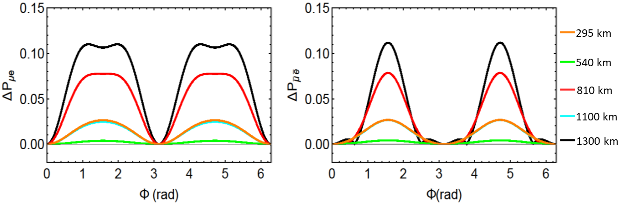
Figure 2: $\Delta P_{\alpha\beta}$ versus $\phi$ in the left panel and $\Delta P_{\bar{\alpha}\bar{\beta}}$ versus $\phi$ in the right panel with $(\alpha,\beta)=(e,\mu)$.

In fig 1, we plot the transition probabilities with respect to the neutrino beam energy E. We plot the appearance probability $P_{\mu e}=P_{\nu_{\mu}\rightarrow\nu_{e}}$ and the disappearance probability $P_{\mu\mu}=P_{\nu_{\mu}\rightarrow\nu_{\mu}}$ of the $\nu_{\mu}$ beam with respect to E, in the top left and right panels respectively. Additionally, in the bottom panel we show $P_{\bar{\nu}_{\mu}\rightarrow\bar{\nu}_{e}}$ and $P_{\bar{\nu}_{\mu}\rightarrow\bar{\nu}_{\mu}}$. The solid lines correspond to $\phi\neq 0$ which represents the non-zero Majorana phase while dashed lines correspond to $\phi=0$ which is the case with Dirac neutrinos. We consider maximal phase $\phi=\pi/2$ as a representative value in these plots. The orange, green, red, cyan and black curves correspond to the probability versus energy E for the baselines 295 km, 540 km, 810 km, 1100 km and 1300 km respectively. As can be seen from the orange curves, in the case of T2K experiment where baseline length is 295 km the dashed curve and the solid curve are almost overlapping with each other, indicating minimal effect of decoherence at this L and E. As the baseline increases, we can see from the green (540 km), red (810 km), cyan (1100 km) and black (1300km) curves that the impact of decoherence increases and reaches maximum for DUNE experiment. However, the ESS$\nu$SB experiment (540 km) and T2HKK (1100 km) are designed to work at the second oscillation maxima i.e. 0.2 GeV and 0.7 GeV respectively. At these energy values one can see negligible difference between the Dirac (solid curve) and Majorana (dashed curve) cases from the green and cyan curves. While the solid and dashed black curves corresponding to DUNE baseline 1300 km show maximum sensitivity to discriminate between Dirac and Majorana phase.

We further study the effect of decoherence on the determination of neutrino nature at the five experiments considered, by defining two quantities $\Delta P_{\alpha\beta}$ and $\Delta{P_{\bar{\alpha}\bar{\beta}}}$. The two quantities $\Delta P_{\alpha\beta}$ and $\Delta{P_{\bar{\alpha}\bar{\beta}}}$ in the case of neutrinos and anti-neutrinos are defined as below

$$\Delta P_{\alpha\beta}=|P_{\nu_{\alpha}\rightarrow\nu_{\beta}}(Dirac)-P_{\nu_{\alpha}\rightarrow\nu_{\beta}}(Majorana)|,$$ (24)

$$\Delta{P_{\bar{\alpha}\bar{\beta}}}=|P_{\bar{\nu}_{\alpha}\rightarrow\bar{\nu}_{\beta}}(Dirac)-P_{\bar{\nu}_{\alpha}\rightarrow\bar{\nu}_{\beta}}(Majorana)|.$$ (25)

The first term in eq. (24) and eq. (25) is obtained by assuming $\phi=0$ while the second is obtained by taking $\phi\subset[0,2\pi]$. When $\alpha=\beta=\mu$ in eq. (24), one can derive that $\Delta P_{\mu\mu}=\Delta P_{\mu e}$ since our analysis is done for two flavour neutrino oscillation picture. Similarly, from eq. (25), we obtain $\Delta P_{\bar{\mu}\bar{\mu}}=\Delta P_{\bar{\mu}\bar{e}}$. Therefore, we numerically obtain two quantities $\Delta P_{\mu e}$ and $\Delta P_{\bar{\mu}\bar{e}}$ with respect to $\phi$ from eq. (24) and eq. (25).

Fig. 2, shows $\Delta P_{\mu e}$ vs $\phi$ in the left panel and $\Delta P_{\bar{\mu}\bar{e}}$ vs $\phi$ in the right panel. To obtain this figure, we fix the peak neutrino beam energy values as per the experimental specifications in table-1 and vary the Majorana phase $\phi\subset[0,2\pi]$. For all non-zero values of $\phi$, the green curve corresponding to the 540 km baseline (ESS$\nu$SB) and the black curve corresponding to the 1300 km baseline (DUNE) show minimum and maximum potential to determine the nature of neutrinos. The green (540 km) and cyan (1100 km) curves show lesser sensitivity to discriminate between Dirac and Majorana neutrinos for all values of $\phi\neq 0$. This can be explained from fig 1, for $\phi=\pi/2$ we have the green, cyan solid (Majorana case) and the dashed (Dirac) curves almost overlapping at the second oscillation maximum. Since, ESS$nu$SB and T2HKK are planned at second oscillation maximum, the effect of decoherence is lesser than that at the first oscillation maxima. For this reason NOvA (810 km) will be more sensitive to determining the nature of neutrinos, next to DUNE as can be seen from the red curve.

IV.2 Non-zero off diagonal elements in $D_{mn}$

In this case, we assume that the decoherence matrix $D_{mn}$ in eq. 9 has two non-zero off-diagonal elements and the diagonal elements are equal i.e. $\alpha=a=c$, $\gamma=0$, $\beta$ and $b$ non-zero. Similar to the previous case, we further obtain the oscillation probabilities under this approximation.

In fig 3, we plot the transition probabilities with respect to the beam energy E. We show the appearance probability $P_{\nu_{\mu}\rightarrow\nu_{e}}$ and the disappearance probability $P_{\nu_{\mu}\rightarrow\nu_{\mu}}$ of the $\nu_{\mu}$ beam with respect to E, in the top left and right panels respectively. In the bottom left(right) panel, we present $P_{\bar{\nu}_{\mu}\rightarrow\bar{\nu}_{e}}$ ($P_{\bar{\nu}_{\mu}\rightarrow\bar{\nu}_{\mu}}$) with respect to anti-neutrino $\bar{\nu_{\mu}}$ beam energy. We assume the neutrino mass ordering as normal ordering. The solid lines correspond to $\phi\neq 0$ which represents the case of non-zero Majorana phase while the dashed lines correspond to $\phi=0$, the Dirac neutrinos. We consider maximal phase $\phi=\pi/2$ as a representative value in these plots. The orange, green, red, cyan and black curves correspond to the probability versus energy E for the baselines 295 km, 540 km, 810 km, 1100 km and 1300 km respectively. In comparison between fig 1 and fig 3, we can see that the additional non-zero off-diagonal elements do not change the probabilities vs E significantly. Accordingly, the conclusions drawn for fig 1, also apply in this case. That is there is maximum difference between the Dirac and the Majorana case for 1300 km baseline when one assumes decoherence in a two flavour neutrino framework. The green and cyan curves corresponding to ESS and T2HKK baselines, show that at second oscillation maxima 0.2 GeV and 0.7 GeV the difference between probabilities for Majorana (solid curve) and Dirac (dashed curve) case is almost negligible.

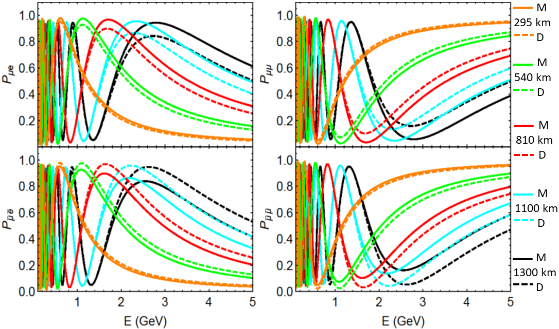
Figure 3: Appearance and disappearance probabilities of neutrinos (upper panel) and anti-neutrinos (lower panel) with respect to energy E (assuming normal mass ordering). The orange, green, red, cyan and black curves correspond to the probability versus energy E for the baselines 295 km, 540 km, 810 km, 1100 km and 1300 km respectively.

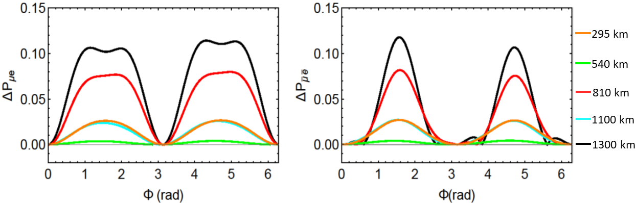
Figure 4: $\Delta P_{\alpha\beta}$ versus $\phi$ in the left panel and $\Delta P_{\bar{\alpha}\bar{\beta}}$ versus $\phi$ in the right panel with $(\alpha,\beta)=(e,\mu)$.

We further obtain $\Delta P_{\mu e}$ and $\Delta{P_{\bar{\mu}\bar{e}}}$ using eq. (24) and eq. (25) respectively, for this case of non-zero off-diagonal elements. In fig 4, we plot $\Delta P_{\mu e}$ vs $\phi$ in the left panel and $\Delta{P_{\bar{\mu}\bar{e}}}$ vs $\phi$ in the right panel. We fix the L and E values as listed in table-1. From the black curve, one can see that for all non-conserving values of $\phi\subset[0,2\pi]$, DUNE shows maximum $\Delta P_{\mu e}$ and $\Delta{P_{\bar{\mu}\bar{e}}}$ values and is followed by NOvA experiment. T2K and T2HKK have same $\Delta P_{\mu e}$ and $\Delta{P_{\bar{\mu}\bar{e}}}$ irrespective of their baselines because T2HKK is planned at second oscillation maxima. From the left plot we note that in the case of neutrino beam, the sensitivity to the Majorana phase is seen for all non-zero values. However for the anti-neutrino beam, the $\Delta{P_{\bar{\mu}\bar{e}}}$ values are non-negligible for smaller range of $\phi$ values ([$0.6\pi$ to $2.6\pi$], [$4\pi$ to $5.6\pi$]).

V Quantum quantifiers

To study a quantum system, it is essential to explore the quantumness of the system. It has been shown that various measures of quantum coherence such as, Bell nolocality clauser1969proposed ; horodecki1995violating ; brunner2014bell , Leggett-Garg inequality (LG-I) leggett1985quantum ; emary2013leggett , entanglement yin2013lower ; blasone2009entanglement , steering inequality wiseman2007steering ; costa2016quantification ; uola2020quantum , non-local advantage of quantum coherence (NAQC) mondal2017nonlocal can be expressed in terms of neutrino oscillation probabilities alok2016quantum ; ming2020quantification and are useful to shed some light on the unknown neutrino oscillation parameters. Recently, some progress has been made where non-classical correlations are defined to analyze charge-parity (CP) violating phase and the neutrino mass hierarchy problem naikoo2020quantum .

In this section, we briefly discuss the various well established measures of quantum correlations and their relations with neutrino oscillation probability. The two flavour neutrino oscillation framework, considered in this work is ideal to study the quantum quantifiers like Bell-CHSH inequality, Steering inequality and non-local advantage of quantum coherence (NAQC), as they are defined for a two-qubit system. We show that these nonclassical entities take different forms for Majorana and Dirac neutrinos. Therefore, one can consider them as potential candidates to probe the nature of neutrinos.

Firstly, we give a brief account of the measures of quantum correlations Bell-CHSH inequality, Steering inequality and NAQC. Later, we numerically obtain these quantities in terms of neutrino oscillation parameters and plot them with respect to the neutrino beam energy E. For analysis purposes we show the results for three baselines, smallest - 295 km, intermediate - 540 km and largest - 1300 km baselines corresponding to T2K, ESS$\nu$SB, DUNE.

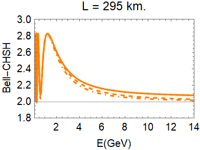
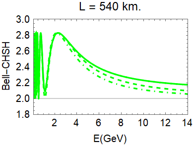
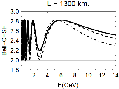
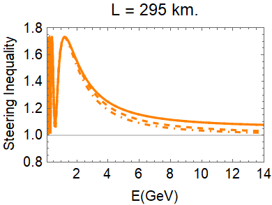
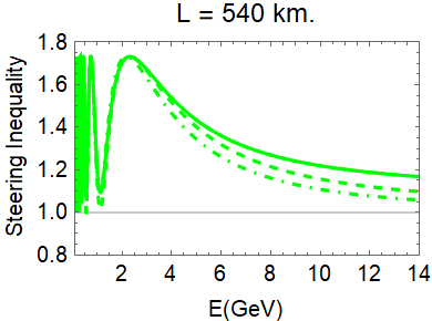
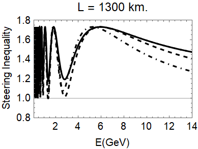
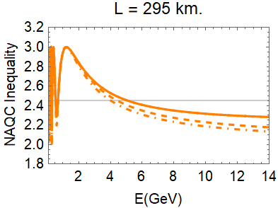
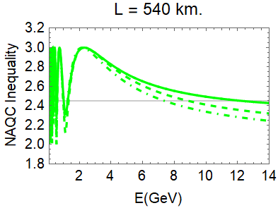
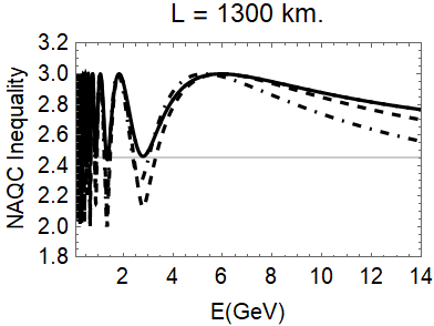
Figure 5: Bell-CHSH inequality versus energy (E) in first row, steering inequality versus energy (E) in second row and NAQC versus energy (E) in third row for T2K (left), ESS$\nu$SB (middle), DUNE (right). Solid line, dashed line and dot-dashed line represents decoherence including matter effect, only matter effect (without decoherence) and vacuum respectively.

Bell-CHSH Inequality : The 2022 Nobel Prize in Physics has been awarded to Alain Aspect, John F. Clauser and Anton Zeilinger for establishing the violation of Bell’s inequalities in experiments with entangled photons. In 1963, it was shown by John Bell that, quantum mechanics is not compatible with local hidden variable theory bell1964einstein . The generalisation of Bell’s theorem presented by Clauser, Horne, Shimony and Holt, to apply on realistic experiment is popularly known as Bell-CHSH inequality clauser1969proposed . This inequality is used to test the quantum correlation between experimentally measurable quantities which are operated on two spatially separated systems. The CHSH inequality in terms of the Bell operator $B_{CHSH}$ is given by

$$|\langle B_{CHSH}\rangle|\leq 2.$$ (26)

The violation of the inequality in eq. (26), can be rewritten in terms of a quantity $M(\rho)=\max_{i\neq j}(u_{i}+u_{j})$ where $u_{i=1,2,3}$ are the eigenvalues of a real matrix $T^{\dagger}T$ (T - correlation matrix)  horodecki1995violating , as

$$|\langle B_{CHSH}\rangle|=2\sqrt{M(\rho)}>2$$ (27)

In the context of two flavour neutrino oscillations, A and B can be considered as neutrinos with two different flavours. The authors of  alok2016quantum have derived $M(\rho)$ in terms of the neutrino oscillation probability $P_{\rm osc}$ and the survival probability $P_{\rm sur}$ as

$$M(\rho) = 1+4P_{\rm sur}P_{\rm osc}~{}.$$ (28)

Therefore, from eq. (27)

$$|\langle B_{CHSH}\rangle|=2\sqrt{1+4P_{osc}P_{sur}}~{}>2.$$ (29)

Steering Inequality : The notion of quantum steering was first proposed by Schrodinger in 1935 schrodinger1935discussion to investigate the Einstein-Podolsky-Rosen (EPR) paradox einstein1935can . In a system with two parties, quantum steering is a phenomenon where one party influences/steers the outcome of a measurement on another party. The steering criteria of a bipartite state $\Gamma_{AB}$ shared between two parties (Alice and Bob) can be diagnosed by an inequality that was developed in a seminal paper by Cavalcanti-Jones-Wiseman-Reid cavalcanti2009experimental . If two parties, both are permitted to measure $n$ observables, then the inequality is formulated as costa2016quantification

$$S_{n}(\Gamma_{AB},\varsigma)=\frac{1}{\sqrt{n}}\left|\sum^{n}_{i=1}\langle A_{i}\otimes B_{i}\rangle\right|\leq 1$$ (30)

with $\langle A_{i}\otimes B_{i}\rangle$ = Tr($\Gamma_{AB}A_{i}\otimes B_{i}$), where $A_{i}={\hat{x}_{i}\cdot\hat{\sigma}}$, $B_{i}={\hat{y}_{i}\cdot\hat{\sigma}}$, $\hat{x}_{i}\in\mathbb{R}^{3}$ are unit vectors, $\hat{y}_{i}\in\mathbb{R}^{3}$ are orthonormal vectors, $\varsigma=\{\hat{x}_{i},...,\hat{x}_{n},\hat{y}_{i},...,\hat{y}_{n}\}$ represents set of measurement directions.

In the case of two flavor neutrino oscillation the steering inequality can be represented as ming2020quantification

$$S_{n}(\Gamma_{AB},\varsigma)=\sqrt{1+8P_{osc}P_{sur}}~{}\leq 1.$$ (31)

Non-local Advantage of Quantum Coherence (NAQC) : Recently, authors in ref. mondal2017nonlocal have proposed a quantifier called non-local advantage of quantum coherence (NAQC). This NAQC parameter is based on $l_{1}$-norm of coherence measure and it represents the quantumness of a system in terms of entanglement and steerability. In ming2020quantification the authors have shown that NAQC acts as a stronger quantifier when compared to Bell-CHSH and steering inequality.

The NAQC-parameter $N_{l_{1}}$ measures the quantumness of a system using steerability and quantum coherence criteria. For a two flavor neutrino system, this parameter can be derived in terms of oscillation ($P_{osc}$) and survival probability ($P_{sur}$) as ming2020quantification

$$N_{l_{1}}=2+2\sqrt{P_{osc}P_{sur}}~{}.$$ (32)

Thus using the above definition of $N_{l_{1}}$, the condition to achieve NAQC for two flavor neutrino system is $N_{l_{1}}\geq 2.45$.

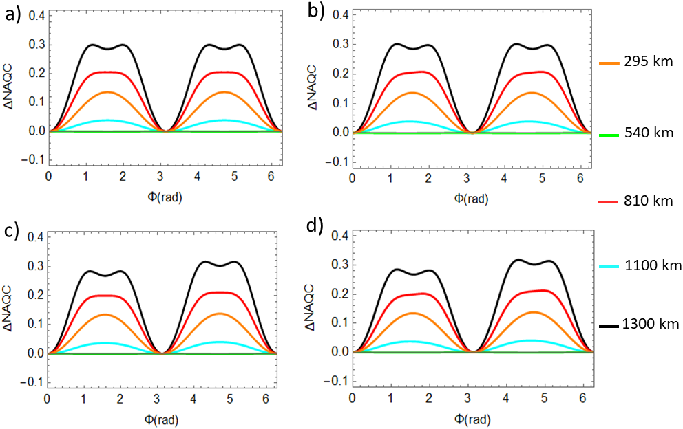
Figure 6: variation of $\Delta NAQC$ as a function of $\phi$ using approximations in fig. 6a. for a diagonal dissipator ($\alpha=a=c$, $\beta=\gamma=b=0$), fig. 6b. one off-diagonal element $\beta$ non zero ($\alpha=a=c$, $\beta=\gamma=0$, $\beta\neq 0$), fig. 6c. one off-diagonal element $b$ non zero ($\alpha=a=c$, $b=\gamma=0$, $b\neq 0$) and in fig. 6d. $\alpha=a=c$, $\gamma=0$, $b$ and $\beta$ non zero

In fig. 5 we present the variation of the Bell-CHSH (top panel), steering inequality (middle panel) and NAQC inequality (bottom panel) with respect to neutrino energy E using eqn. (29), eqn. (31) and eqn. (32) to investigate the quantumness of neutrino oscillations. The oscillation and the decoherence parameters considered are listed in table 2. In each row, we show the plots for three different baselines 295 km (left), 540 km (middle) and 1300 km (right). The solid lines in each plot are obtained by considering the neutrino propagation over a distance L, assuming decoherence and matter interactions while the dashed and the dot-dashed lines correspond to the cases of neutrino propagation with matter effect (no decoherence) and propagation in vacuum respectively. From the first row of fig 5, it can be seen that the Bell-CHSH inequality is violated i.e. $B_{CHSH}\geq 2$, for all E values in the case of all the three baselines. Second row of fig 5 shows that the flavor states violate steering inequality i.e. $S_{3}\geq 1$ for all the energies in the case of T2K, ESS$\nu$SB and DUNE baselines. However, in the third row it is illustrated that NAQC i.e. $N_{l_{1}}\geq 2.45$ is not achieved for some energy ranges by the neutrino flavor states in the case of all the three baselines. Hence, neutrino flavour states attaining NAQC can also achieve Bell nonlocality and quantum steering. NAQC can be considered as a stronger quantifier than steering and Bell-CHSH quantity to reveal the quantumness of the neutrino system. Similar conclusions have been reported by Fei Ming et al ming2020quantification examining the neutrino oscillations in vacuum. Basing on this conclusion, we consider the NAQC quantifier as a better candidate to throw some light on the nature of neutrinos.

From eq. (19) and eq. (32) it is obvious that ${N}_{l_{1}}$ is a function of the Majorana phase ($\phi$). When we consider $\phi=0$ we can obtain $P_{osc}$ and thus ${N}_{l_{1}}$ for the case of Dirac neutrinos. Here we propose a candidate $\Delta NAQC$, to determine the nature of neutrinos

$$\Delta NAQC=|N_{l_{1}}(Dirac)-N_{l_{1}}(Majorana)|.$$ (33)

We use the same values for the oscillation and decoherence parameters to calculate $\Delta NAQC$, as given in table II. In fig 6 we plot $\Delta NAQC$ as a function of $\phi$ imposing some extra conditions on decoherence parameters. We consider the following combinations for the sake of completeness: in fig 6a both $\beta$ and $b$ are zero (only non-zero diagonal elements); in fig 6b, $\beta$ is non-zero and $b$ is zero (one non-zero off-diagonal element); in fig 6c $b$ is non-zero and $\beta$ is zero (one non-zero off-diagonal element); and in fig 6d both $\beta$ and $b$ are non-zero (two non-zero off-diagonal elements). The orange, green, red, cyan and black lines are assigned for T2K, ESS$\nu$SB, NOvA, T2HKK and DUNE experiments respectively. In fig 6, the $\Delta NAQC$ values in the presence of decoherence indicate that one can probe the nature of neutrinos using DUNE, NOvA and T2K but the possibility is low for the baselines T2HKK and ESS$\nu$SB. Additionally, it is visible from fig 6 that the $\Delta NAQC$ for 295 km baseline (orange curve) shows more sensitivity to the nature of neutrinos when compared to $\Delta P_{\mu e}$ plotted in fig 2 and fig 4. Thus reinforcing the conclusion that NAQC, quantum quantifiers in general, can be used as a measure to understand the nature of neutrinos.

VI Conclusions

We analyse the two flavour neutrino oscillations in matter in a dissipative environment, by assuming two scenarios for the decoherence matrix. Firstly, for simplicity, we consider the case where we have non-zero diagonal elements and zero off-diagonal elements in the decoherent matrix. Whereas in the second case, we assume non-zero diagonal and non-zero off-diagonal elements. In these two scenarios, we see that the transition probabilities depend explicitly on the Majorana phase $\phi$. We further study the oscillations of Dirac and Majorana neutrinos at L (baseline) and E (neutrino beam energy) values corresponding to five long-baseline neutrino oscillation experiments T2K, NOvA, ESS$\nu$SB, T2HKK and DUNE. We find that, in principle, one can probe the nature of neutrinos at these experiments under the assumption that neutrino subsystem interacts with the environment. Moreover, we extend our analysis to estimate the quantum correlations in the system using quantifiers - Bell-CHSH, steering and NAQC for these L, E values. We note that the neutrino flavour states achieving NAQC attain Bell-CHSH, steering inequalities for all E. Thus, we consider NAQC as a stronger quantifier for a quantum system and analyse its sensitivity to the nature of neutrinos. The NAQC quantifier carries different values for Majorana and Dirac neutrinos. Hence, the non-vanishing difference $\Delta NAQC$ can be used to discriminate between Dirac and Majorana neutrinos. In the presence of matter effect, a dissipative matrix presents non-vanishing $\Delta NAQC$, which in principle allows us to differentiate between the Dirac and Majorana neutrinos at neutrino oscillation experiments.

Acknowledgements: K. N. Deepthi would like to thank DST-SERB SIRE program for the financial support to visit Indiana University, Bloomington, Indiana, USA.

References

- (1) J. Vergados, H. Ejiri, F. Šimkovic, Theory of neutrinoless double-beta decay, Reports on Progress in Physics 75 (10) (2012) 106301.
- (2) S. Bilenky, C. Giunti, Neutrinoless double-beta decay: a probe of physics beyond the standard model, International Journal of Modern Physics A 30 (04n05) (2015) 1530001.
- (3) Z. Collaboration, et al., First search for the majorana nature of neutrinos in the inverted mass ordering region with kamland-zen, arXiv preprint arXiv:2203.02139 (2022).
- (4) Y. Farzan, T. Schwetz, A. Y. Smirnov, Reconciling results of lsnd, miniboone and other experiments with soft decoherence, Journal of High Energy Physics 2008 (07) (2008) 067.
- (5) R. Oliveira, M. Guzzo, Quantum dissipation in vacuum neutrino oscillation, The European Physical Journal C 69 (3) (2010) 493–502.
- (6) P. Bakhti, Y. Farzan, T. Schwetz, Revisiting the quantum decoherence scenario as an explanation for the lsnd anomaly, Journal of High Energy Physics 2015 (5) (2015) 1–16.
- (7) M. M. Guzzo, P. C. de Holanda, R. L. Oliveira, Quantum dissipation in a neutrino system propagating in vacuum and in matter, Nuclear Physics B 908 (2016) 408–422.
- (8) G. B. Gomes, M. Guzzo, P. De Holanda, R. Oliveira, Parameter limits for neutrino oscillation with decoherence in kamland, Physical Review D 95 (11) (2017) 113005.
- (9) A. Capolupo, S. M. Giampaolo, G. Lambiase, Decoherence in neutrino oscillations, neutrino nature and cpt violation, Physics Letters B 792 (2019) 298–303.
- (10) S. W. Hawking, The Unpredictability of Quantum Gravity, Commun. Math. Phys. 87 (1982) 395–415.
- (11) S. W. Hawking, Virtual black holes, Phys. Rev. D 53 (1996) 3099–3107.
- (12) S. W. Hawking, Wormholes in Space-Time, Phys. Rev. D 37 (1988) 904–910.
- (13) S. W. Hawking, C. J. Hunter, Gravitational entropy and global structure, Phys. Rev. D 59 (1999) 044025.
- (14) J. R. Ellis, N. E. Mavromatos, D. V. Nanopoulos, String theory modifies quantum mechanics, Phys. Lett. B 293 (1992) 37–48.
- (15) J. R. Ellis, N. E. Mavromatos, D. V. Nanopoulos, CPT violation in string modified quantum mechanics and the neutral kaon system, Int. J. Mod. Phys. A 11 (1996) 1489–1508.
- (16) F. Benatti, R. Floreanini, Damped harmonic oscillators in the holomorphic representation, J. Phys. A 33 (2000) 8139.
- (17) F. Benatti, R. Floreanini, Massless neutrino oscillations, Physical Review D 64 (8) (2001) 085015.
- (18) M. Richter, B. Dziewit, J. Dajka, Leggett-garg k 3 quantity discriminates between dirac and majorana neutrinos, Physical Review D 96 (7) (2017) 076008.
- (19) L. Buoninfante, A. Capolupo, S. M. Giampaolo, G. Lambiase, Revealing neutrino nature and cpt violation with decoherence effects, The European Physical Journal C 80 (11) (2020) 1–11.
- (20) J. Carrasco-Martínez, F. Díaz, A. Gago, Uncovering the majorana nature through a precision measurement of the cp phase, Physical Review D 105 (3) (2022) 035010.
- (21) V. Gorini, A. Frigerio, M. Verri, A. Kossakowski, E. Sudarshan, Properties of quantum markovian master equations, Reports on Mathematical Physics 13 (2) (1978) 149–173.
- (22) D. Manzano, A short introduction to the lindblad master equation, Aip Advances 10 (2) (2020) 025106.
- (23) K. Abe, N. Abgrall, H. Aihara, T. Akiri, J. Albert, C. Andreopoulos, S. Aoki, A. Ariga, T. Ariga, S. Assylbekov, et al., T2k neutrino flux prediction, Physical Review D 87 (1) (2013) 012001.
- (24) H.-K. Proto-Collaboration, K. Abe, K. Abe, S. Ahn, H. Aihara, A. Aimi, R. Akutsu, C. Andreopoulos, I. Anghel, L. Anthony, et al., Physics potentials with the second hyper-kamiokande detector in korea, Progress of Theoretical and Experimental Physics 2018 (6) (2018) 063C01.
- (25) Y. Itow, T. Kajita, K. Kaneyuki, M. Shiozawa, Y. Totsuka, Y. Hayato, T. Ishida, T. Ishii, T. Kobayashi, T. Maruyama, et al., The jhf-kamioka neutrino project, arXiv preprint hep-ex/0106019 (2001).
- (26) E. Baussan, M. Dracos, T. Ekelof, E. F. Martinez, H. Ohman, N. Vassilopoulos, The use of a high intensity neutrino beam from the ess proton linac for measurement of neutrino cp violation and mass hierarchy, arXiv preprint arXiv:1212.5048 (2012).
- (27) R. Acciarri, M. Acero, M. Adamowski, C. Adams, P. Adamson, S. Adhikari, Z. Ahmad, C. Albright, T. Alion, E. Amador, et al., Long-baseline neutrino facility (lbnf) and deep underground neutrino experiment (dune) conceptual design report, volume 4 the dune detectors at lbnf, arXiv preprint arXiv:1601.02984 (2016).
- (28) J. F. Clauser, M. A. Horne, A. Shimony, R. A. Holt, Proposed experiment to test local hidden-variable theories, Physical review letters 23 (15) (1969) 880.
- (29) R. Horodecki, P. Horodecki, M. Horodecki, Violating bell inequality by mixed spin-12 states: necessary and sufficient condition, Physics Letters A 200 (5) (1995) 340–344.
- (30) N. Brunner, D. Cavalcanti, S. Pironio, V. Scarani, S. Wehner, Bell nonlocality, Reviews of Modern Physics 86 (2) (2014) 419.
- (31) A. J. Leggett, A. Garg, Quantum mechanics versus macroscopic realism: Is the flux there when nobody looks?, Physical Review Letters 54 (9) (1985) 857.
- (32) C. Emary, N. Lambert, F. Nori, Leggett–garg inequalities, Reports on Progress in Physics 77 (1) (2013) 016001.
- (33) J. Yin, Y. Cao, H.-L. Yong, J.-G. Ren, H. Liang, S.-K. Liao, F. Zhou, C. Liu, Y.-P. Wu, G.-S. Pan, et al., Lower bound on the speed of nonlocal correlations without locality and measurement choice loopholes, Physical Review Letters 110 (26) (2013) 260407.
- (34) M. Blasone, F. Dell’Anno, S. De Siena, F. Illuminati, Entanglement in neutrino oscillations, EPL (Europhysics Letters) 85 (5) (2009) 50002.
- (35) H. M. Wiseman, S. J. Jones, A. C. Doherty, Steering, entanglement, nonlocality, and the einstein-podolsky-rosen paradox, Physical review letters 98 (14) (2007) 140402.
- (36) A. Costa, R. Angelo, Quantification of einstein-podolsky-rosen steering for two-qubit states, Physical Review A 93 (2) (2016) 020103.
- (37) R. Uola, A. C. Costa, H. C. Nguyen, O. Gühne, Quantum steering, Reviews of Modern Physics 92 (1) (2020) 015001.
- (38) D. Mondal, T. Pramanik, A. K. Pati, Nonlocal advantage of quantum coherence, Physical Review A 95 (1) (2017) 010301.
- (39) A. K. Alok, S. Banerjee, S. U. Sankar, Quantum correlations in terms of neutrino oscillation probabilities, Nuclear Physics B 909 (2016) 65–72.
- (40) F. Ming, X.-K. Song, J. Ling, L. Ye, D. Wang, Quantification of quantumness in neutrino oscillations, The European Physical Journal C 80 (3) (2020) 1–9.
- (41) J. Naikoo, A. K. Alok, S. Banerjee, S. U. Sankar, G. Guarnieri, C. Schultze, B. C. Hiesmayr, A quantum information theoretic quantity sensitive to the neutrino mass-hierarchy, Nuclear Physics B 951 (2020) 114872.
- (42) J. S. Bell, On the einstein podolsky rosen paradox, Physics Physique Fizika 1 (3) (1964) 195.
- (43) E. Schrödinger, Discussion of probability relations between separated systems, in: Mathematical Proceedings of the Cambridge Philosophical Society, Vol. 31, Cambridge University Press, 1935, pp. 555–563.
- (44) A. Einstein, B. Podolsky, N. Rosen, Can quantum-mechanical description of physical reality be considered complete?, Physical review 47 (10) (1935) 777.
- (45) E. G. Cavalcanti, S. J. Jones, H. M. Wiseman, M. D. Reid, Experimental criteria for steering and the einstein-podolsky-rosen paradox, Physical Review A 80 (3) (2009) 032112.