A joint model of the individual mean and within-subject variability of a longitudinal outcome with a competing risks time-to-event outcome

Abstract

Motivated by recent findings that within-subject (WS) visit-to-visit variabilities of longitudinal biomarkers can be strong risk factors for health outcomes, this paper introduces and examines a new joint model of a longitudinal biomarker with heterogeneous WS variability and competing risks time-to-event outcome. Specifically, our joint model consists of a linear mixed-effects multiple location-scale submodel for the individual mean trajectory and WS variability of the longitudinal biomarker and a semiparametric cause-specific Cox proportional hazards submodel for the competing risks survival outcome. The submodels are linked together via shared random effects. We derive an expectation-maximization algorithm for semiparametric maximum likelihood estimation and a profile-likelihood method for standard error estimation. We implement efficient computational algorithms that scales to biobank-scale data with tens of thousands of subjects. Our simulation results demonstrate that, in the presence of heterogeneous WS variability, the proposed method has superior performance for estimation, inference, and prediction, over the classical joint model with homogeneous WS variability. An application of our method to a Multi-Ethnic Study of Atherosclerosis (MESA) data reveals that there is substantial heterogeneity in systolic blood pressure (SBP) WS variability across MESA individuals and that SBP WS variability is an important predictor for heart failure and death, (independent of, or in addition to) the individual SBP mean level. Furthermore, by accounting for both the mean trajectory and WS variability of SBP, our method leads to a more accurate dynamic prediction model for heart failure or death. A user-friendly R package JMH is developed and publicly available at https://github.com/shanpengli/JMH.

, , , , , and

1 Introduction

In biomedical studies, it is often of interest to study the temporal patterns of longitudinal biomarkers and their association with health outcomes. This paper studies a new joint model of a longitudinal biomarker and a time-to-event outcome that takes into account of possible heterogeneous within-subject (WS) variability of the longitudinal biomarker. Our research is motivated by recent evidence that the WS visit-to-visit variations of some longitudinal biomarkers for diabetes patients are strong risk factors for various health outcomes (Rothwell et al., 2010; Zhou et al., 2018; Ceriello, Monnier and Owens, 2019). For example, using several clinical trials, including UK Prospective Diabetes Study (UKPDS) (Group et al., 1998), Action to Control Cardiovascular Risk in Diabetes (ACCORD) (Group, 2008; Zhou et al., 2018; Ismail-Beigi et al., 2010), and Veterans Affairs Diabetes Trial (VADT) (Duckworth et al., 2009; Reaven et al., 2019), several investigators have demonstrated that individual glycemic variability and blood pressure variability were associated with the risk of cardiovascular diseases (CVD), e.g., myocardial infarction or stroke (Zhou et al., 2018; Nuyujukian et al., 2021), heart failure (Nuyujukian et al., 2020), nephropathy (Zhou et al., 2020, 2021), and retinopathy (Zhou et al., 2021), independent of traditional glycemic and blood pressure control. These studies typically used an ad hoc two-stage approach that first estimates the individual variability of a longitudinal biomarker in the stage 1 analysis and then correlates the individual variability from stage 1 with a time-to-event outcome in the stage 2 analysis. However, the ad hoc two-stage approach has some obvious practical and theoretical drawbacks and limitations.

To illustrate, in a two-stage analysis, participants may be excluded if they have insufficient repeated measures of a biomarker to generate reliable estimates of visit-to-visit variability during the first stage. Second, the first stage analysis is unable to account for the variability measures’ uncertainty caused by the uneven number of repeated measures across individuals. Additionally, the first stage analysis cannot adjust for time-varying effects, such as medication, during variability estimation, leading to significant estimation bias and inaccurate inference during the second stage’s risk assessment. Lastly, the second stage analysis cannot perform dynamic prediction of event of interest relying on the underlying trajectory of biomarker(s) as time-dependent covariates. As a result, there is a pressing need to develop a comprehensive statistical framework that can simultaneously model the individual mean and within-subject variability trends of a longitudinal biomarker, allowing for valid statistical inference on their connections with a time-to-event outcome. Furthermore, this framework should enable dynamic prediction of the event outcome based on the observed biomarker history.

During the past three decades, joint modeling of longitudinal and time-to-event data has been extensively studied in the statistical literature and has emerged as a versatile tool to address many challenging issues in longitudinal and survival data analysis. For instance, joint models have been used to handle non-ignorable missing data due to a terminal event in longitudinal data analysis, model intermittently observed time-varying covariates and/or measurement error in survival analysis, and make dynamic prediction of a time-to-event outcome based on the observed trajectories of longitudinal biomarkers (Tsiatis and Davidian, 2004; Wu et al., 2012; Elashoff et al., 2016; Hickey et al., 2018; Papageorgiou et al., 2019; Alsefri et al., 2020; Huang et al., 2011). However, current statistical literature on joint models of longitudinal and time-to-event data has mostly focused on modeling the mean attribute of a longitudinal biomarker trajectory and its association with a time-to-event outcome and typically assume homogeneous WS variability for the longitudinal biomarker. More recently, there have been efforts to model a longitudinal biomarker while accounting for heterogeneous WS variability (Hedeker, Mermelstein and Demirtas, 2008; Dzubur et al., 2020; German et al., 2021; Parker et al., 2021). Hedeker, Mermelstein and Demirtas (2008) introduced a mixed-effects location-scale model for the longitudinal data, which allows both WS and between-subject (BS) variabilities to be modeled by time-dependent covariates. Dzubur et al. (2020) further extended the mixed-effects location-scale model to mixed-effects multiple location-scale models that allow for multiple random effects in the mean component. German et al. (2021) developed a robust and scalable estimation method to study the effects of both time-varying and time-invariant predictors on WS variability. Parker et al. (2021) proposed a joint modeling approach to associate both mean trajectory and WS variability of systolic blood pressure with left ventricular mass in early adulthood. However, these longitudinal models have some major limitations. They rely on the stringent missing at random (MAR) assumption, which is often violated by non-ignorable missing data due to a terminal event. Moreover, they are not formally linked to an event outcome and thus cannot be readily used to study the association between a longitudinal biomarker with an event outcome of interest. As mentioned above, joint modeling of longitudinal and time-to-event outcomes can help to address these limitations. However, to the best of our knowledge, joint models of longitudinal and survival outcomes in the presence of heterogeneous WS variability have not yet been reported.

This paper aims to fill the above-mentioned gap in the statistical literature on joint models. The newly developed joint models can capture distinct attributes in a longitudinal biomarker’s mean and WS variability and link them to a time-to-event outcome. We illustrate the utility of our method using data from the Multi-Ethnic Study of Atherosclerosis (MESA). The new joint model consists of a linear mixed-effects multiple location scale submodel for the mean and WS variability of a longitudinal biomarker and a semiparametric cause-specific Cox proportional hazards submodel for a competing risks survival outcome. The submodels are linked by shared random effects. We derive an expectation-maximization (EM) algorithm for semiparametric maximum likelihood parameter estimation and adopt a profile-likelihood approach for standard error estimation. We also develop an efficient implementation of our procedure that scales to large-scale biobank data. To this end, we point out that the EM algorithm and standard error estimation for our semiparametric joint model will require $O(n^{2})$ and $O(n^{3})$ operations, respectively, when implemented naively due to repetitive risk set calculations (see Appendix C). By developing customized linear scan algorithms for both the EM algorithm and standard error estimation, we reduce the computational complexity to $O(n)$ and thus make the implementation scalable to massive sample size data with tens of thousands to millions of subjects. Furthermore, our empirical results show that in the presence of heterogeneous WS variability, a classical joint model with homogeneous WS variability can lead to biased estimation and invalid inference, which can be remedied by our proposed joint model (see Table 1). Finally, we have developed a user-friendly R package JMH for the proposed methodology and made it publicly available at https://github.com/shanpengli/JMH.

The rest of the paper is organized as follows. Section 2 describes the semiparametric shared random effects joint model framework and derives an efficient, customized EM algorithm for semiparametric maximum likelihood estimation and a standard error estimation method. Section 3 evaluates the empirical performance of the proposed joint model in contrast to a classical joint model via simulation studies. In Section 4, we apply our developed method to the MESA study. Concluding remarks and further discussion are given in Section 5.

2 Methods

2.1 Model and data specifications

Assume that there are $n$ subjects in the study. For subject $i$, one observes a longitudinal outcome $Y_{i}(t)$ at multiple time points $t_{ij}$, $j=1,\ldots,n_{i}$, $i=1,\ldots,n$. In addition, each subject may experience one of $K$ distinct failure types or be right censored during follow-up. Let $\tilde{T}_{i}$ denote the failure time of interest, $\tilde{D}_{i}$ the failure type taking values in $\{1,\ldots,K\}$, and $C_{i}$ be a censoring time for subject $i$. Then the observed right-censored competing risks time-to-event data for subject $i$ has the form $(T_{i},D_{i})\equiv\left\{\text{min}(\tilde{T}_{i},C_{i}),\tilde{D}_{i}I(\tilde{T}_{i}\leq C_{i})\right\}$, $i=1,\ldots,n$.

Assume that the longitudinal outcome $Y_{i}(t)$ is characterized by the following mixed-effects multiple location-scale submodel:

$$Y_{i}(t) = m_{i}(t)+\sigma_{i}(t)\epsilon_{i}(t),$$ (1)

$$m_{i}(t) = X_{i}^{(1)T}(t)\beta+Z_{i}^{T}(t)b_{i},$$ (2)

$$\sigma_{i}^{2}(t) = \exp\left\{W_{i}^{T}(t)\tau+V_{i}^{T}(t)\omega_{i}\right\},$$ (3)

where $X_{i}^{(1)}(t)$, $Z_{i}(t)$, $W_{i}(t)$, and $V_{i}(t)$ are vectors of possibly time-varying covariates, $\beta$ and $b_{i}$ represent the fixed effects and random effects, respectively, associated with the location component $m_{i}(t)$ for the mean trajectory, and $\tau$ and $\omega_{i}$ represent the fixed effects and random effects, respectively, associated with the scale component $\sigma_{i}(t)$ for the WS variability. Assume that the measurement error $\epsilon_{i}(t)\sim N(0,1)$ is independent of $b_{i}$ and $\omega_{i}$, and mutually independent across all time points and subjects, and the random effects $\theta_{i}\equiv(b_{i}^{T},\omega_{i}^{T})^{T}$ follow a multivariate normal distribution $MVN(0,\Sigma_{\theta})$ with mean 0 and variance-covariance matrix

$$\Sigma_{\theta}=\left({\begin{array}[]{cc}\Sigma_{bb}&\Sigma_{b\omega}\\ \Sigma_{b\omega}^{T}&\Sigma_{\omega\omega}\\ \end{array}}\right),$$

where $\Sigma_{b\omega}=cov(b_{i},\omega_{i})$, $\Sigma_{bb}=cov(b_{i},b_{i})$, and $\Sigma_{\omega\omega}=cov(\omega_{i},\omega_{i})$.

Assume further that the competing risks time-to-event outcome follows the following cause-specific Cox proportional hazards submodel:

$$\lambda_{k}(t\mid X_{i}^{(2)}(t),M_{i}(\theta_{i},t)) = \lim_{h\to 0}\frac{P(t\leq\tilde{T}_{i}<t+h,\tilde{D}_{i}=k\mid T_{i}\geq t,X_{i}^{(2)}(t),M_{i}(\theta_{i},t))}{h}$$ (5)

$$= \lambda_{0k}(t)\exp\{X_{i}^{(2)T}(t)\gamma_{k}+M_{i}^{T}(\theta_{i},t)\alpha_{k}\},\quad k=1,\ldots,K,$$ (6)

where $\lambda_{0k}(t)$ is a completely unspecified baseline hazard function, $X_{i}^{(2)}(t)$ is a vector of possibly time-varying covariates for the competing risks time-to-event outcome, $\gamma_{k}$ is a vector of fixed effects of $X_{i}^{(2)}(t)$, $M_{i}(\theta_{i},t)$ is a vector of pre-specified functions of $\theta_{i}$ and $t$, and $\alpha_{k}$ is a vector of association parameters between the longitudinal and time-to-event outcomes.

Note that the three submodels (1)-(6) are linked together via the latent association structure $M_{i}^{T}(\theta_{i},t)\alpha_{k}$. Some useful examples of $M_{i}^{T}(\theta_{i},t)\alpha_{k}$ include (1) “shared random effects” parameterization: $M_{i}^{T}(\theta_{i},t)\alpha_{k}=\alpha_{bk}^{T}b_{i}+\alpha_{\omega k}^{T}\omega_{i}$, (2) “present value” parameterization: $M_{i}^{T}(\theta_{i},t)\alpha_{k}=\alpha_{bk}m_{i}(t)+\alpha_{\omega k}\log\left\{\sigma_{i}^{2}(t)\right\}$, and (3) “present value of latent process” parametrization: $M_{i}^{T}(\theta_{i},t)\alpha_{k}=\alpha_{bk}Z_{i}^{T}(t)b_{i}+\alpha_{\omega k}V_{i}^{T}(t)\omega_{i}$, where $\alpha_{bk}$ and $\alpha_{\omega k}$ are the association parameters for the individual mean trajectory and WS variability, respectively. It is also worth noting that our joint model (1)-(6) reduces to the joint model of Li et al. (2022) if the submodel (3) is replaced by a homogeneous WS variance $\sigma_{i}^{2}(t)\equiv\sigma^{2}$.

Throughout the paper we assume that $C_{i}$ is independent of $\tilde{T}_{i}$ conditional on the observed covariates and the unobserved random effects $\theta_{i}$, $i=1,\ldots,n.$ We further assume that the longitudinal measurements are independent of the competing risks time-to-event data conditional on the observed covariates and the unobserved random effects.

2.2 Likelihood and EM estimation

Denote by $\Psi$ = ($\beta$, $\tau$, $\gamma$, $\alpha$, $\Sigma_{\theta}$, $\lambda_{01}(\cdot)$, …, $\lambda_{0K}(\cdot)$) the collection of all unknown parameters and functions from the submodels (1)-(6), where $\gamma=(\gamma_{1}^{T},\ldots,\gamma_{K}^{T})^{T}$ and $\alpha=(\alpha_{b1}^{T},\ldots,\alpha_{bK}^{T},\alpha_{\omega 1}^{T},\ldots,\alpha_{\omega K}^{T})^{T}$. Denote by $Y_{i}=(Y_{i1},...,Y_{in_{i}})^{T}$, where $Y_{ij}=Y_{i}(t_{ij})$. Omitting the covariates for the sake of brevity, the observed-data likelihood is given by

$$L(\Psi;Y,T,D) \propto \prod_{i=1}^{n}f(Y_{i},T_{i},D_{i}\mid\Psi)$$

$$= \prod_{i=1}^{n}\int f(Y_{i}\mid\theta_{i},\Psi)f(T_{i},D_{i}\mid\theta_{i},\Psi)f(\theta_{i}\mid\Psi)d\theta_{i}$$

$$= \prod_{i=1}^{n}\int\prod_{j=1}^{n_{i}}\frac{1}{\sqrt{2\pi\sigma_{i}^{2}(t_{ij})}}\exp\left[-\frac{\left\{Y_{i}(t_{ij})-m_{i}(t_{ij})\right\}^{2}}{2\sigma_{i}^{2}(t_{ij})}\right]$$

$$\times\prod_{k=1}^{K}\lambda_{k}\left\{T_{i}\mid X_{i}^{(2)}(T_{i}),M_{i}(\theta_{i},T_{i})\right\}^{I(D_{i}=k)}$$

$$\times\exp\left[-\sum_{k=1}^{K}\int_{0}^{T_{i}}\lambda_{k}\left\{t\mid X_{i}^{(2)}(t),M_{i}(\theta_{i},t)\right\}dt\right]$$

$$\times\frac{1}{\sqrt{(2\pi)^{q}\mid\Sigma_{\theta}\mid}}\exp\left(-\frac{1}{2}\theta_{i}^{T}\Sigma_{\theta}^{-1}\theta_{i}\right)d\theta_{i},$$

where the first equality follows from the assumption that $Y_{i}$ and $(T_{i},D_{i})$ are independent conditional on the covariates and the random effects.

Because $\Psi$ involves $K$ unknown hazard functions, directly maximizing the above observed-data likelihood is difficult. To tackle this issue, we derive an EM algorithm to compute the semiparametric maximum likelihood estimate (SMLE) of $\Psi$ by regarding the latent random effects $\theta_{i}$ as missing data (Dempster, Laird and Rubin, 1977; Elashoff, Li and Li, 2008).The complete-data likelihood based on $(Y,T,D,\theta)$ is given by

$$L(\Psi;Y,T,D,\theta) \propto \prod_{i=1}^{n}\prod_{j=1}^{n_{i}}\frac{1}{\sqrt{2\pi\exp\left\{W_{i}^{T}(t_{ij})\tau+V_{i}(t_{ij})^{T}\omega_{i}\right\}}}$$

$$\times\exp\left[-\frac{\left\{Y_{i}(t_{ij})-X_{i}^{(1)T}(t_{ij})\beta-Z_{i}^{T}(t_{ij})b_{i}\right\}^{2}}{2\exp\left\{W_{i}^{T}(t_{ij})\tau+V_{i}(t_{ij})^{T}\omega_{i}\right\}}\right]$$

$$\times\prod_{k=1}^{K}\left[\Delta\Lambda_{0k}(T_{i})\exp\left\{X_{i}^{(2)T}(T_{i})\gamma_{k}+M_{i}^{T}(\theta_{i},T_{i})\alpha_{k}\right\}\right]^{I(D_{i}=k)}$$

$$\times\exp\left[-\sum_{k=1}^{K}\int_{0}^{T_{i}}\exp\left\{X_{i}^{(2)T}(t)\gamma_{k}+M_{i}^{T}(\theta_{i},t)\alpha_{k}\right\}d\Lambda_{0k}(t)\right]$$

$$\times\frac{1}{\sqrt{(2\pi)^{q}\mid\Sigma_{\theta}\mid}}\exp\left(-\frac{1}{2}\theta_{i}^{T}\Sigma_{\theta}^{-1}\theta_{i}\right),$$

where $\Lambda_{0k}(.)$ is the cumulative baseline hazard function for type $k$ failure and $\Delta\Lambda_{0k}(T_{i})=\Lambda_{0k}(T_{i})-\Lambda_{0k}(T_{i}-)$. The EM algorithm iterates between an expectation step (E-step):

$$Q(\Psi;\Psi^{(m)})\equiv E^{(m)}_{\theta\mid Y,T,D,\Psi^{(m)}}\left\{\log L(\Psi;Y,T,D,\theta)\right\},$$ (7)

and a maximization step (M-step):

$$\Psi^{(m+1)}=\arg\max_{\Psi}Q(\Psi;\Psi^{(m)}),$$ (8)

until the algorithm converges, where $\Psi^{(m)}$ is the estimate of $\Psi$ from the $m$-th iteration. Each E-step involves calculating integrals of the form

$$E^{(m)}\{h(\theta_{i})\} = \int h(\theta_{i})f(\theta_{i}\mid Y_{i},T_{i},D_{i},\Psi^{(m)})d\theta_{i}$$ (9)

for every subject $i$, $i=1,\ldots,n$, which are evaluated using the standard Gauss-Hermite quadrature rule (Press et al., 2007). As shown in Appendix A.1, the M-step (8) has closed-form solutions for a number of parameters including the nonparametric baseline cumulative hazard functions $\Lambda_{0k}(t)$, $k=1,\ldots,K$, which is a key advantage of the EM-algorithm. Other parameters without closed-form solutions in the M-step are updated using the one-step Newton-Raphson method. Details of the EM algorithm are provided in equations (45)-(59) of the Appendix.

2.3 Standard error estimation

As discussed in Elashoff et al. (2016) (Section 4.1, p.72), several approaches including profile-likelihood, observed information matrix, and bootstrap method have been proposed in the literature for estimating the standard errors of the parametric components of the SMLE. Here we adopt the profile-likelihood approach because it can be readily computed from the EM algorithm and performed well in our simulation studies. Let $\Omega=(\beta,\tau,\gamma,\alpha,\Sigma_{\theta})$ denote the parametric component of $\Psi$ and $\hat{\Omega}$ its SMLE. We propose to estimate the variance-covariance matrix of $\hat{\Omega}$ by inverting the empirical Fisher information obtained from the profile likelihood of $\Omega$ (Lin, McCulloch and Rosenheck, 2004; Zeng et al., 2005; Zeng and Cai, 2005) as follows:

$$\sum_{i=1}^{n}[\nabla_{\Omega}l^{(i)}(\hat{\Omega};Y,T,D)][\nabla_{\Omega}l^{(i)}(\hat{\Omega};Y,T,D)]^{T},$$ (10)

where $\nabla_{\Omega}l^{(i)}(\hat{\Omega};Y,T,D)$ is the observed score vector from the profile-likelihood $l^{(i)}({\Omega};Y,T,D)$ of $\Omega$ on the $i$th subject by profiling out the baseline hazards. Details of the observed score vector for each parametric component are provided in equations (61)-(74) of the Appendix.

Remark.

We point out in Appendix C that a naive implementation of the proposed EM algorithm and the standard error estimate for our joint model typically involves $O(n^{2})$ and $O(n^{3})$ operations, respectively, which will become computationally prohibitive for large scale studies with a massive number of subjects. However, by applying the linear scan algorithms of Li et al. (2022), one can reduce the computational complexity of our EM algorithm and standard error estimation to $O(n)$ for the shared random effects joint model (1)-(6), where $X_{i}^{(2)}(t)$ is assumed to be time-independent and $M_{i}^{T}(\theta_{i},t)\alpha_{k}$ = $\alpha_{bk}^{T}b_{i}+\alpha_{\omega k}^{T}\omega_{i}$. We have implemented these efficient algorithms and developed an R package, JMH (https://github.com/shanpengli/JMH), which is capable of fitting the aforementioned shared random effects joint model in real time with tens of thousands patients.

2.4 Dynamic prediction for competing risks time-to-event data

The proposed joint model (1)-(6) not only offers a general framework to model the individual mean and WS variability of a longitudinal outcome and study their association with a competing risks time-to-event outcome, but also facilitates subject-level dynamic prediction of cumulative incidence probabilities of a competing risks event for a new subject $i^{*}$ based on the longitudinal outcome history. Specifically, given the longitudinal outcome history $Y_{i^{*}}^{(s)}=\{Y_{i^{*}}(t_{{i^{*}}j}),t_{{i^{*}}j}\leq s\}$ prior to a landmark time $s>0$ and that an event has yet to happen by time $s$, the cumulative incidence probability for type $k$ failure at a horizon time $u>s$ is given by

$$P_{i^{*}k}(u,s|\Psi) = \text{Pr}(T_{i^{*}}\leq u,D_{i^{*}}=k|T_{i^{*}}>s,Y_{i^{*}}^{(s)},\Psi)$$ (11)

$$= \int\text{Pr}(T_{i^{*}}\leq u,D_{i^{*}}=k|T_{i^{*}}>s,Y_{i^{*}}^{(s)},\theta_{i^{*}},\Psi)f(\theta_{i^{*}}|T_{i^{*}}>s,Y_{i^{*}}^{(s)},\Psi)d\theta_{i^{*}}$$ (12)

$$= \int\text{Pr}(T_{i^{*}}\leq u,D_{i^{*}}=k|T_{i^{*}}>s,\theta_{i^{*}},\Psi)f(\theta_{i^{*}}|T_{i^{*}}>s,Y_{i^{*}}^{(s)},\Psi)d\theta_{i^{*}}$$ (13)

$$= \int\frac{\text{Pr}(T_{i^{*}}\leq u,D_{i^{*}}=k,T_{i^{*}}>s|\theta_{i^{*}},\Psi)}{\text{Pr}(T_{i^{*}}>s|\theta_{i^{*}},\Psi)}f(\theta_{i^{*}}|T_{i^{*}}>s,Y_{i^{*}}^{(s)},\Psi)d\theta_{i^{*}}$$ (14)

$$= \int\frac{CIF_{i^{*}k}(u,s|\theta_{i^{*}},\Psi)}{S_{i^{*}}(s|\theta_{i^{*}},\Psi)}f(\theta_{i^{*}}|T_{i^{*}}>s,Y_{i^{*}}^{(s)},\Psi)d\theta_{i^{*}}$$ (15)

$$= \frac{\int\frac{CIF_{i^{*}k}(u,s|\theta_{i^{*}},\Psi)}{S_{i^{*}}(s|\theta_{i^{*}},\Psi)}f(Y_{i^{*}}^{(s)}|\theta_{i^{*}},\Psi)f(T_{i^{*}}>s|\theta_{i^{*}},\Psi)f(\theta_{i^{*}}|\Psi)d\theta_{i^{*}}}{\int f(Y_{i^{*}}^{(s)}|\theta_{i^{*}},\Psi)f(T_{i^{*}}>s|\theta_{i^{*}},\Psi)f(\theta_{i^{*}}|\Psi)d\theta_{i^{*}}},$$ (16)

where $S_{i^{*}}(.)=\exp\left\{-\sum_{k=1}^{K}\int_{0}^{s}d\Lambda_{k}(t|\theta_{i^{*}},\Psi)\right\}$ is the overall survival function and $CIF_{i^{*}k}(.)=\int_{s}^{u}S_{i^{*}}(t|\theta_{i^{*}},\Psi)d\Lambda_{k}(t|\theta_{i^{*}},\Psi)$ the cumulative incidence function (CIF) for type $k$ failure and the last step of integral (16) can be evaluated using a standard Gauss-Hermite quadrature rule. An estimate of $P_{i^{*}k}(u,s|\Psi)$ can be obtained by replacing $S_{i^{*}}(.)$, $CIF_{i^{*}k}(.)$, and $\Psi$ by their sample estimates $\hat{S}_{i^{*}}(.)$, $\widehat{CIF}_{i^{*}k}(.)$, and $\hat{\Psi}$, respectively.

3 Simulation studies

We present extensive simulations to examine the finite sample performance of the proposed joint model with heterogeneous WS variability for the longitudinal outcome. We also demonstrate that ignoring heterogeneous WS variability can lead to biased parameter estimates, biased standard error estimates, invalid inferences, and inferior prediction accuracy.

We first evaluate the performance of parameter estimation, standard error estimation, and confidence intervals in comparison to a classical joint model that ignores heterogeneous WS variability. In this simulation, the longitudinal measurements $Y_{i}(t_{ij})$ were generated from the mixed-effects multiple location scale model (1)-(3) with

$$m_{i}(t_{ij}) = \beta_{0}+\beta_{1}X_{1i}+\beta_{2}X_{2i}+\beta_{3}X_{3i}+\beta_{4}t_{ij}+b_{i},$$ (17)

$$\sigma_{i}^{2}(t_{ij}) = \exp(\tau_{0}+\tau_{1}X_{1i}+\tau_{2}X_{2i}+\tau_{3}X_{3i}+\tau_{4}t_{ij}+\omega_{i}),$$ (18)

and the competing risks event data were generated from the following proportional cause-specific hazards models:

$$\lambda_{1}(t) = \lambda_{01}(t)\exp\{\gamma_{11}X_{1i}+\gamma_{12}X_{2i}+\gamma_{13}X_{3i}+\alpha_{b1}b_{i}+\alpha_{\omega 1}\omega_{i}\},$$ (19)

$$\lambda_{2}(t) = \lambda_{02}(t)\exp\{\gamma_{21}X_{1i}+\gamma_{22}X_{2i}+\gamma_{23}X_{3i}+\alpha_{b2}b_{i}+\alpha_{\omega 2}\omega_{i}\},$$ (20)

where the four sub-models (17)-(20) are linked together through the shared random effects $\theta_{i}=(b_{i},\omega_{i})^{T}$. Here $t_{ij}$’s represent the scheduled visiting times for subject $i$ with an increment of 0.25, $X_{1i}\sim Bernoulli(0.5)$, $X_{2i}\sim Uni(-1,1)$, and $X_{3i}\sim N(1,4)$. $\theta_{i}\sim N_{2}(0,\Sigma_{\theta})$, with $\sigma_{b}^{2}=0.5,\sigma_{\omega}^{2}=0.5,\text{ and }\sigma_{b\omega}=\sigma_{b}\sigma_{\omega}\rho_{bw}$. The WS variance $\sigma_{i}^{2}(t_{ij})$ modeled by equation (18) includes a fixed effect induced by a time-varying covariate $t_{ij}$ (visit-to-visit variation), three covariates $X_{i1},X_{i2}$, and $X_{i3}$, and a subject level random effect $\omega_{i}$. The baseline hazards $\lambda_{01}(t),\lambda_{02}(t)$ are set to constants 0.05 and 0.1, respectively. We simulated non-informative censoring time $C_{i}\sim Uni(4,8)$ and let $T_{i}=min\{T_{i1}^{*},T_{i2}^{*},C_{i}\}$ be the observed survival time (possibly censored) for subject $i$, where $T_{i1}^{*}$ and $T_{i2}^{*}$ are independent event times from models (19) and (20), respectively, $i=1,\ldots,n$. The longitudinal measurements for subject $i$ are assumed missing when $t_{ij}>T_{i}$. The censoring rate is about 24%, the rate of event 1 is about 43%, and the rate of event 2 is about 33%. The average number of longitudinal measurements per subject is around 10.

Table 1: Comparison of the bias, standard error (SE), estimated standard error (Est. SE), and coverage probability (CP) between the proposed joint model with heterogeneous WS variability (Model 1) and a classical joint model with homogeneous WS variability (Model 2) for the longitudinal outcome ($n=800$)

		Model 1 (heterogeneous WS variability)				Model 2 (homogeneous WS variability)
Parameter	True	Bias	SE	Est. SE	CP (%)	Bias	SE	Est. SE	CP (%)
$Longitudinal$
Fixed effects
Mean trajectory
$\beta_{0}$	5	0.004	0.051	0.048	93.8	$<$0.001	0.055	0.066	97.0
$\beta_{1}$	1.5	-0.007	0.065	0.070	95.8	-0.012	0.067	0.075	96.0
$\beta_{2}$	2	$<$0.001	0.064	0.060	92.2	-0.005	0.066	0.066	94.8
$\beta_{3}$	1	$<$0.001	0.019	0.018	93.8	-0.004	0.021	0.020	93.6
$\beta_{4}$	2	$<$0.001	0.003	0.003	95.2	-0.001	0.004	0.004	89.4
WS variability
$\tau_{0}$	0.5	$<$0.001	0.051	0.052	94.0	-	-	-	-
$\tau_{1}$	0.5	-0.001	0.068	0.067	95.6	-	-	-	-
$\tau_{2}$	-0.2	-0.001	0.058	0.058	93.8	-	-	-	-
$\tau_{3}$	0.2	$<$0.001	0.017	0.018	94.8	-	-	-	-
$\tau_{4}$	0.05	$<$0.001	0.003	0.003	95.6	-	-	-	-
$Competing\ risks$
Fixed effects
$\gamma_{11}$	1	0.007	0.144	0.144	95.8	-0.085	0.133	0.134	90.0
$\gamma_{12}$	0.5	0.007	0.118	0.119	94.8	-0.007	0.111	0.110	95.8
$\gamma_{13}$	0.5	0.003	0.042	0.042	96.4	-0.031	0.039	0.038	85.2
$\gamma_{21}$	-0.5	-0.003	0.156	0.153	94.4	-0.006	0.166	0.156	94.0
$\gamma_{22}$	0.5	0.002	0.133	0.130	94.2	0.018	0.135	0.131	94.2
$\gamma_{23}$	0.25	0.002	0.040	0.040	95.2	0.002	0.041	0.041	96.2
Association
$\alpha_{b1}$	1	-0.001	0.200	0.195	94.4	0.045	0.190	0.162	90.0
$\alpha_{b2}$	-1	-0.015	0.187	0.188	95.8	-0.360	0.266	0.222	66.8
$\alpha_{\omega 1}$	0.5	0.013	0.153	0.163	97.2	-	-	-	-
$\alpha_{\omega 2}$	-0.5	-0.018	0.165	0.172	96.0	-	-	-	-
Covariance matrix
of random effects
$\sigma_{b}^{2}$	0.5	-0.005	0.050	0.047	91.6	-0.015	0.059	0.052	89.8
$\sigma_{b\omega}$	0.25	-0.002	0.036	0.035	93.2	-	-	-	-
$\sigma_{\omega}^{2}$	0.5	-0.004	0.044	0.044	94.6	-	-	-	-

Note: Large error in confidence interval coverage probability (CP) compared to the 95% nominal level are highlighted in boldface. Each entry is based on 500 Monte Carlo samples.

We fitted both our proposed joint model (1)-(6) with heterogeneous WS variability (Model 1) using our developed methods and R package “JMH” as described in Section 2 and a classical joint model (Model 2) with homogeneous WS variance ($\sigma_{i}^{2}(t_{ij})\equiv\sigma^{2}$) using the R-package FastJM (Li et al., 2022). Table 1 summarizes simulated results on the bias, sample standard deviations of the parameter estimates (SE), average estimated standard errors of the parameter estimates (Est. SE), and coverage probabilities of 95% confidence intervals (CP) for a scenario with medium correlation ($\rho_{b\omega}=0.50$) between the random effects, and sample size $n=800$. Each entry in the table is based on 500 Monte Carlo samples.

In Table 1, our proposed joint model method (Model 1) demonstrates a smaller bias for all parameters and standard error estimates and that CPs are close to the 95% nominal level. On the other hand, ignoring the heterogeneous WS variability (Model 2) induced non-negligible bias in some parameter and standard error estimates, leading to significant under-coverage of the associated confidence intervals. For example, the parameter estimate and standard error estimate of $\alpha_{b2}$ are both substantially biased, and its associated confidence interval coverage probability (66.8%) is unreasonably low compared to the 95% nominal level.

We have performed additional simulations with different sample sizes and random effects correlations. The results are consistent with those in Table 1 and thus are not included here.

4 An application: Multi-Ethnic Study of Atherosclerosis (MESA)

The Multi-Ethnic Study of Atherosclerosis (MESA) started in July 2000 and included a community-based sample of 6,814 men and women, who were aged 45-84 years, free of clinical CVD events at baseline, and constituted four racial/ethnic groups from six US field centers (Bild et al., 2002). The first examination was assigned at the enrollment (i.e., baseline), and the following exams were conducted with up to five exams in total. During the study, blood pressures, i.e., systolic and diastolic blood pressure (SBP and DBP, mmHg), were measured at each exam, and the event surveillance was completely separate from the exams, from phone follow-ups at intervals of 9-12 months. Eligible events such as CVD were collected and abstracted for central adjudication. As an illustration, we consider joint modeling of longitudinal SBP with two competing risk time-to-event outcomes: heart failure (risk 1) and death (risk 2). We adjust for age at baseline (in years), sex (1=female, 0=male), and race (1=non-white, 0=white) in both SBP and competing risk time-to-event models. After excluding 29 individuals missing the event time, a cohort of 6,785 participants with an average of 4.3 SBP measures per subject and a total of 29,283 SBP measures are kept for analysis. Among them, 380 (5.6%) participants had heart failure, 1,327 (19.6%) died, and 5,078 (74.8%) were right censored without experiencing any of the two events.

In our joint model (Model 1), the longitudinal SBP ($Y_{i}(t_{ij})$) is assumed to follow the mixed-effects multiple location scale model (1)-(3) as

$$m_{i}(t_{ij}) = \beta_{0}+\beta_{1}t_{ij}+\beta_{2}\text{Age}_{i}+\beta_{3}\text{Race}_{i}+\beta_{4}\text{Sex}_{i}+b_{i},$$ (21)

$$\sigma_{i}^{2}(t_{ij}) = \exp(\tau_{0}+\tau_{1}t_{ij}+\tau_{2}\text{Age}_{i}+\tau_{3}\text{Race}_{i}+\tau_{4}\text{Sex}_{i}+\omega_{i}),$$ (22)

and the competing risk outcomes, heart failure, and death are modeled by the following cause-specific hazards model:

$$\lambda_{1}(t) = \lambda_{01}(t)\exp(\gamma_{11}\text{Age}_{i}+\gamma_{12}\text{Race}_{i}+\gamma_{13}\text{Sex}_{i}+\alpha_{b1}b_{i}+\alpha_{\omega 1}\omega_{i}),$$ (23)

$$\lambda_{2}(t) = \lambda_{02}(t)\exp(\gamma_{21}\text{Age}_{i}+\gamma_{22}\text{Race}_{i}+\gamma_{23}\text{Sex}_{i}+\alpha_{b2}b_{i}+\alpha_{\omega 2}\omega_{i}),$$ (24)

where the shared random effects $\theta_{i}=(b_{i},\omega_{i})^{T}$ follow bivariate normal distribution with mean zero and variance-covariance matrix

$$\Sigma_{\theta}=\left({\begin{array}[]{cc}\sigma_{b}^{2}&\sigma_{b\omega}\\ \sigma_{b\omega}&\sigma_{\omega}^{2}\\ \end{array}}\right).$$

Several more complex models were also explored, including additional covariate adjustment, their interactions, and random slopes. The results are similar; thus, we only report results for the shared random intercept model in Table 2. For comparison purposes, Table 2 also includes an analysis based on the following classical joint model (Model 2) of SBP, heart failure, and death, assuming homogeneous SBP WS variability:

$$Y_{i}(t_{ij}) = m_{i}(t_{ij})+\sigma\epsilon(t_{ij}),$$ (26)

$$m_{i}(t_{ij}) = \beta_{0}+\beta_{1}t_{ij}+\beta_{2}\text{Age}_{i}+\beta_{3}\text{Race}_{i}+\beta_{4}\text{Sex}_{i}+b_{i},$$ (27)

$$\lambda_{1}(t) = \lambda_{01}(t)\exp(\gamma_{11}\text{Age}_{i}+\gamma_{12}\text{Race}_{i}+\gamma_{13}\text{Sex}_{i}+\alpha_{b1}b_{i}),$$ (28)

$$\lambda_{2}(t) = \lambda_{02}(t)\exp(\gamma_{21}\text{Age}_{i}+\gamma_{22}\text{Race}_{i}+\gamma_{23}\text{Sex}_{i}+\alpha_{b2}b_{i}),$$ (29)

and Model 3 where we assume homogeneous individual mean trajectory and heterogeneous WS variability of SBP:

$$m_{i}(t_{ij}) = \beta_{0}+\beta_{1}t_{ij}+\beta_{2}\text{Age}_{i}+\beta_{3}\text{Race}_{i}+\beta_{4}\text{Sex}_{i},$$ (30)

$$\sigma_{i}^{2}(t_{ij}) = \exp(\tau_{0}+\tau_{1}t_{ij}+\tau_{2}\text{Age}_{i}+\tau_{3}\text{Race}_{i}+\tau_{4}\text{Sex}_{i}+\omega_{i}),$$ (31)

$$\lambda_{1}(t) = \lambda_{01}(t)\exp(\gamma_{11}\text{Age}_{i}+\gamma_{12}\text{Race}_{i}+\gamma_{13}\text{Sex}_{i}+\alpha_{\omega 1}\omega_{i}),$$ (32)

$$\lambda_{2}(t) = \lambda_{02}(t)\exp(\gamma_{21}\text{Age}_{i}+\gamma_{22}\text{Race}_{i}+\gamma_{23}\text{Sex}_{i}+\alpha_{\omega 2}\omega_{i}),$$ (33)

Table 2: Joint analysis of systolic blood pressure (SBP, mmHg), time to heart failure, and time to death using the MESA data (Model 1 is the joint model (21)-(24) assuming heterogeneous SBP individual mean trajectory and heterogeneous WS variability, Model 2 is the joint model (26)-(29) assuming heterogeneous SBP individual mean trajectory and homogeneous SBP WS variability, and Model 3 is the joint model (30)-(33) assuming homogeneous SBP individual mean trajectory and heterogeneous SBP WS variability. Abbreviations: SE=standard error; HR=hazard ratio; CI=confidence interval.)

	Model 1		Model 2	Model 3
Longitudinal outcome	Mean trajectory	WS variability	Mean trajectory	Mean trajectory	WS variability
(Systolic blood pressure (SBP, mmHg))	Estimate (SE)	Estimate (SE)	Estimate (SE)	Estimate (SE)	Estimate (SE)
Intercept	79.59 (0.74)***	2.34 (0.08)***	79.55 (1.31)***	78.05 (0.45)***	3.85 (0.09)***
Time (Years from baseline)	-0.02 (0.03)	0.08 ($<$0.01)***	-0.14 (0.03)***	-0.05 (0.05)	0.02 ($<$0.01)***
Age at baseline	0.66 (0.01)***	0.03 ($<$0.01)***	0.67 (0.02)***	0.67 ($<$0.01)***	0.02 ($<$0.01)***
Race (Non-White/White)	6.58 (0.24)***	0.23 (0.02)***	5.95 (0.41)***	5.44 (0.13)***	0.20 (0.03)***
Sex (Female/Male)	-0.22 (0.26)	0.24 (0.03)***	0.89 (0.42)*	-0.63 (0.26)*	0.29 (0.03)***
Sex $\times$ Time	0.26 (0.04)***	-0.02 (0.01)**	0.21 (0.04)***	0.18 (0.07)**	-0.02 ($<$0.01)*
Random effects
(variance-covariance matrix)	Estimate (SE)		Estimate (SE)	Estimate (SE)
$\sigma_{b}^{2}$	204.15 (4.45)***		213.49 (5.42)***	N/A
$\sigma_{b\omega}$	7.34 (0.23)***		N/A	N/A
$\sigma_{\omega}^{2}$	0.46 (0.02)***		N/A	0.54 (0.02)***
Cause-specific hazard
(Heart failure)	HR (95% CI)		HR (95% CI)	HR (95% CI)
Age at baseline	1.08 (1.07-1.10)***		1.08 (1.07-1.09)***	1.08 (1.07-1.09)***
Race (Non-White/White)	1.00 (0.81-1.23)		0.96 (0.78-1.18)	0.98 (0.79-1.21)
Sex (Female/Male)	0.57 (0.46-0.70)***		0.58 (0.47-0.71)***	0.61 (0.49-0.74)***
Random effects
Mean trajectory ($\alpha_{b1}$)	0.99 (0.97-1.01)		1.03 (1.02-1.03)***	N/A
WS variability ($\alpha_{\omega 1}$)	$2.04^{+}$ (1.42-2.94)***		N/A	$1.70^{+}$ (1.47-1.98)***
Cause-specific hazard
(Death)	HR (95% CI)		HR (95% CI)	HR (95% CI)
Age at baseline	1.11 (1.10-1.12)***		1.10 (1.10-1.11)***	1.11 (1.10-1.11)***
Race (Non-White/White)	1.11 (0.99-1.24)		1.08 (0.97-1.21)	1.09 (0.97-1.22)
Sex (Female/Male)	0.64 (0.57-0.71)***		0.64 (0.58-0.72)***	0.65 (0.58-0.73)***
Random effects
Mean trajectory ($\alpha_{b2}$)	0.98 (0.97-0.99)***		1.01 (1.00-1.01)***	N/A
WS variability ($\alpha_{\omega 2}$)	$1.91^{+}$ (1.55-2.35)***		N/A	$1.33^{+}$ (1.22-1.46)***

* p-value$<$0.05; ** p-value$<$0.01; *** p-value$<$0.001.

⁺ Standardized HR of association parameter for WS variability is reported to show the effect on the cause-specific hazard by 1 SD change of WS variability of SBP.

There are several interesting observations from the results (Table 2). Our proposed model (Model 1) reveals that the heterogeneity of SBP WS variability is substantial ($\sigma_{\omega}^{2}=0.46,\mbox{SE}=0.02$, p-value$<0.001$) across MESA individuals. It also suggests that standardized SBP WS variability ($\omega_{i}/\sigma_{\omega}$) is highly predictive of heart failure (HR = 2.04, 95% CI=(1.42, 2.94)) and death (HR = 1.91, 95% CI=(1.55, 2.35)). As SBP WS variability ($\omega_{i}$) and individual mean ($b_{i}$) are two highly correlated covariates, caution needs to be taken when interpreting their effects. In contrast, Model 2 only relates subject-specific SBP to the event outcomes besides the baseline covariates. Results of Model 2 show that every 10 mmHg elevation of subject-specific SBP contributes to 34% and 10% increased risk of heart failure and death, respectively. Model 3 only relates WS variability of SBP to the event outcomes besides the baseline covariates. Similar to Model 1, results of Model 3 also suggests that standardized SBP WS variability ($\omega_{i}/\sigma_{\omega}$) is highly predictive of heart failure (HR = 1.70, 95% CI=(1.47, 1.98)) and death (HR = 1.33, 95% CI=(1.22, 1.46)).

Next, we assess and compare the dynamic prediction accuracy of Model 1, Model 2, and Model 3 using a 4-fold cross-validated mean absolute prediction error (MAPE4) by contrasting the predicted and empirical cumulative incidence rates for competing risk $k$ ($k=1,2$) as defined below.

1. Randomly partition all the MESA in study subjects into $4$ equal-sized disjoint subsets, $\mathcal{D}_{n}^{(1)},\ldots,\mathcal{D}_{n}^{(4)}$.

2. For each $l=1,\ldots,4$, designate $\mathcal{D}_{n}^{(l)}$ as the validation set and the remaining $3$ subsets, denoted by $\mathcal{D}_{n}^{(-l)}$, as the training set. The training set $\mathcal{D}_{n}^{(-l)}$ is used to fit a joint model, and then for each subject $i^{*}$ in the validation set $\mathcal{D}_{n}^{(l)}$, the fitted model is used to perform a dynamic prediction of its risk-$k$ cumulative incidence rate $\hat{P}_{i^{*}k}(u,s)$ at a horizon time $u$ from some landmark time $s$ using formula (11).

3. Rank the subjects in the validation $\mathcal{D}_{n}^{(l)}$ according to the predicted risk $k$ cumulative incidence rate $\hat{P}^{(l)}_{i^{*}k}(u,s)$, and denote by $Q_{kq}^{(l)}$ the $q^{th}$ quartile group, $q=1,\ldots,4$. Define the risk $k$ mean absolute prediction error (MAPE) for the $q^{th}$ quartile group $Q_{kq}^{(l)}$ by

   $${\text{MAPE}^{(l)}_{k}}(u,s)=\frac{1}{4}\sum_{q=1}^{4}\Bigg{|}\hat{F}_{k}(u|s,Q_{kq}^{(l)})-\frac{\sum I(i^{*}\in Q_{kq}^{(l)})\hat{P}_{i^{*}k}(u,s)}{\sum I(i^{*}\in Q_{kq}^{(l)})}\Bigg{|},$$ (34)

   where $\hat{F}_{k}(u|s,Q_{kq}^{(l)})=\int_{s}^{u}\hat{S}(t|s,Q_{kq}^{(l)})d\hat{H}_{k}(t|s,Q_{kq}^{(l)})$ is the empirical cumulative risk $k$ incidence in the $q^{th}$ quartile group $Q_{kq}^{(l)}$, with $\hat{S}(t|s,Q_{kq}^{(l)})$ being the Kaplan-Meier estimator of the all risk survival function and $\hat{H}_{k}(t|s,Q_{kq}^{(l)})$ the Nelson-Aalen estimator of the risk $k$ cause-specific cumulative hazard function within the $q^{th}$ quartile group.

4. Lastly, the 4-fold cross-validated mean absolute prediction error (MAPE4) for risk $k$ is defined as

   $${\text{MAPE4}_{k}}(u,s) = \frac{1}{4}\sum_{l=1}^{4}{\text{MAPE}^{(l)}_{k}}(u,s),\quad k=1,2.$$

Figure 1 depicts the 4-fold cross-validated MAPE4 score with landmark time $s=7$ and horizon times $u=9,11$, and 13 years from baseline for heart failure (risk 1) and death (risk 2). Figure 1b demonstrated that Model 1 outperforms both Model 2 and Model 3 for dynamic prediction of the risk of death at all three horizon times $u=$9, 11, and 13, with substantially smaller MAPE4 prediction error. Although Model 3 yielded a smaller prediction error than Model 1 and Model 2 for predicting heart failure in the MESA cohort, these results should be interpreted with caution. Given the incidence rate of heart failure is low ($<6\%$), MAPE4 may not be an informative prediction accuracy measure.

Figure 2 provides an illustration of the significant impact of SBP WS variability on the event outcomes. In Figure 2, we ranked all subjects by the empirical Bayes estimate of the random effect $\omega_{i}$ based on Model 1 and then plotted the cumulative incidence of heart failure (Figure 2a) and death (Figure 2b) for the top 20% high SBP WS variability group versus the bottom 20% low SBP WS variability group. Our results demonstrate participants in the top 20% high SBP WS variability group had a much higher cumulative incidence than the bottom 20% low SBP WS variability group for both clinical events. The same phenomenon is also observed in the spaghetti profile plot of the longitudinally measured SBP for 25 randomly selected participants from each group over the study period, as shown in Figure 3, where both events are more likely to happen among the high WS variability cohort than the low WS variability cohort.

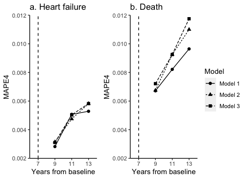
Figure 1: The average 4-fold cross-validated MAPE4 score at $s=7$ and $u=(9,11,13)$ years from baseline based on 10 random splits. Model 1 is the joint model (21)-(24) assuming heterogeneous SBP individual mean trajectory and heterogeneous WS variability, Model 2 is the joint model (26)-(29) assuming heterogeneous SBP individual mean trajectory and homogeneous SBP WS variability, and Model 3 is the joint model (30)-(33) assuming homogeneous SBP individual mean trajectory and heterogeneous SBP WS variability.

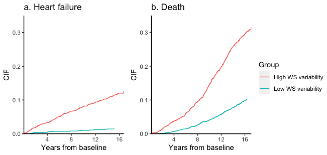
Figure 2: Empirical cause-specific cumulative incidence function (CIF) of the high (top 20%, red) and low (bottom 20%, blue) WS variability of SBP (mmHg) groups for heart failure (left) and death (right) in MESA data.

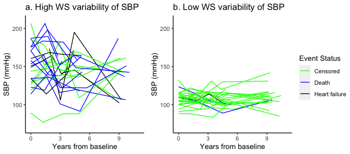
Figure 3: Spaghetti profile plot of 25 randomly selected participants from the high (top 20%, left) and low (bottom 20%, right) SBP WS variability groups in the MESA cohort.

5 Discussion

Current literature on joint models of longitudinal and time-to-event outcomes has focused primarily on modeling the mean trajectory of a longitudinal biomarker and associating it with a time-to-event outcome. To our knowledge, the joint model introduced in this paper is the first to model both the individual mean and WS variability of a longitudinal biomarker and to utilize both features for dynamic prediction of the time-to-event outcomes. We have developed an EM algorithm for SMLE, a profile-likelihood method for standard error estimation, and scalable linear scan algorithms for large data. The advantages of our proposed model over classical joint modeling approach are demonstrated using simulations as well as through an application to the MESA study. Our analysis of the MESA study not only reveals that the SBP WS variability is another important predictor for heart disease besides the SBP mean level but also leads to a better dynamic prediction model for heart failure and death by accounting for the mean and WS variability of SBP in the joint model.

The utility of joint modeling of mean trajectory and WS variability of a longitudinal biomarker with a time-to-event outcome is not limited to the simple setting considered in this paper. It could be informative to extend the current work to many other applications, including joint models with multiple longitudinal biomarkers, multivariate time-to-event outcomes, recurrent events, and other types of time-to-event data such as left-truncated or interval-censored data. Extensions to more flexible models for the time trend of the longitudinal outcome are also warranted.

It should be noted that the estimation method based on the EM algorithm may become computationally infeasible as the number of random effects, the number of longitudinal measurements, or the number of subjects increases. For example, the EM algorithm involves numerically evaluating multiple intractable integrals for all subjects in each EM iteration, and the computational cost of the standard Gauss Hermite quadrature rule used in this paper for numerical integration grows exponentially with the number of random effects. In future research, further development of scalable estimation methods is warranted.

Lastly, our model and inference procedure are based on normality assumptions for both the random effects and WS error term in the longitudinal submodel. It would be of interest to develop more robust joint models and inference procedure in future research.

6 Software

A user-friendly R package JMH to fit the shared parameter joint model developed in this paper is publicly available at https://github.com/shanpengli/JMH.

Appendix A The EM algorithm

A.1 The M-step (equation (8))

It can be shown that the parameters $\beta$, $\Sigma_{\theta}$, as well as $\Lambda_{0k}(t_{kj})$ at the $q_{k}$ distinct observed type $k$ event times $t_{k1}>\cdots>t_{kq_{k}}$, have closed form solutions in the M-step. Using $E^{(m)}$ to denote $E^{(m)}_{b_{i},\omega_{i}|Y_{i},T_{i},D_{i},\Psi^{(m)}}$ and $a^{\bigotimes 2}=aa^{T},\;\forall a\in\mathbb{R}^{d}$, we have

$$\beta^{(m+1)} = \left\{\sum_{i=1}^{n}\sum_{j=1}^{n_{i}}\frac{X_{i}^{(1)\bigotimes 2}(t_{ij})}{\exp\left\{W_{i}^{T}(t_{ij})\tau^{(m)}\right\}}E^{(m)}\left[\exp\left\{-V_{i}(t_{ij})^{T}\omega_{i}\right\}\right]\right\}^{-1}$$ (37)

$$\times\left(\sum_{i=1}^{n}\sum_{j=1}^{n_{i}}\frac{E^{(m)}\left[\exp\left\{-V_{i}(t_{ij})^{T}\omega_{i}\right\}\right]X_{i}^{(1)}(t_{ij})Y_{i}(t_{ij})}{\exp\left\{W_{i}^{T}(t_{ij})\tau^{(m)}\right\}}\right.$$

$$\left.-\frac{Z_{i}^{T}(t_{ij})E^{(m)}\left[b_{i}\exp\left\{-V_{i}(t_{ij})^{T}\omega_{i}\right\}\right]X_{i}^{(1)}(t_{ij})}{\exp\left\{W_{i}^{T}(t_{ij})\tau^{(m)}\right\}}\right)$$

$$\Sigma_{\theta}^{(m+1)} = \frac{1}{n}\sum_{i=1}^{n}E^{(m)}(\theta_{i}^{\bigotimes 2})=\frac{1}{n}\sum_{i=1}^{n}\left({\begin{array}[]{cc}E^{(m)}(b_{i}^{\bigotimes 2})&E^{(m)}(b_{i}\omega_{i}^{T})\\ E^{(m)}(\omega_{i}b_{i}^{T})&E^{(m)}(\omega_{i}^{\bigotimes 2})\\ \end{array}}\right),$$ (40)

$$\Lambda_{0k}^{(m+1)}(t_{kj}) = \sum_{l=j}^{q_{k}}\frac{d_{kl}}{\sum_{r\in R(t_{kj})}\exp\left\{X_{r}^{(2)T}(t_{kj})\gamma_{k}^{(m)}\right\}E^{(m)}\left[\exp\left\{M_{i}^{T}(\theta_{i},t_{kj})\alpha_{k}\right\}\right]},$$ (41)

where $R(t_{kj})$ is the risk set at time $t_{kj}$, and $d_{kl}$ is the number of type $k$ failures at time $t_{kl}$, for $k=1,\ldots,K.$

The other parameters $\tau$, $\gamma$, $\alpha$, and $\nu$ do not have closed form solutions and we update them using the one-step Newton-Raphson method

$$\tau^{(m+1)} = \tau^{(m)}+I_{\tau}^{(m)-1}U_{\tau}^{(m)},$$

$$\gamma_{k}^{(m+1)} = \gamma_{k}^{(m)}+I_{\gamma_{k}}^{(m)-1}U_{\gamma_{k}}^{(m)},\quad k=1,\ldots,K,$$

$$\alpha_{k}^{(m+1)} = \alpha_{k}^{(m)}+I_{\alpha_{k}}^{(m)-1}U_{\alpha_{k}}^{(m)},\quad k=1,\ldots,K,$$

where

$$I_{\tau}^{(m)} = \sum_{i=1}^{n}\sum_{j=1}^{n_{i}}\frac{1}{2}\exp\left\{-W_{i}^{T}(t_{ij})\tau^{(m)}\right\}$$ (45)

$$\times\left(r_{i}^{(m+1)2}(t_{ij})E^{(m)}\left[\exp\left\{-V_{i}(t_{ij})^{T}\omega_{i}\right\}\right]\right.$$

$$-\left.2r_{i}^{(m+1)}(t_{ij})Z_{i}^{T}(t_{ij})E^{(m)}\left[b_{i}\exp\left\{-V_{i}(t_{ij})^{T}\omega_{i}\right\}\right]\right.$$

$$+\left.\text{tr}\left[Z_{i}^{\bigotimes 2}(t_{ij})E^{(m)}\left\{b_{i}^{\bigotimes 2}\exp\left\{-V_{i}(t_{ij})^{T}\omega_{i}\right\}\right\}\right]\right)W_{i}^{\bigotimes 2}(t_{ij}),$$

$$U_{\tau}^{(m)} = \sum_{i=1}^{n}\sum_{j=1}^{n_{i}}\frac{1}{2}\left[\exp\left\{-W_{i}^{T}(t_{ij})\tau^{(m)}\right\}\right.$$ (49)

$$\times\left.\left\{r_{i}^{(m+1)2}(t_{ij})E^{(m)}\left[\exp\left\{-V_{i}(t_{ij})^{T}\omega_{i}\right\}\right]\right.\right.$$

$$-\left.\left.2r_{i}^{(m+1)}(t_{ij})Z_{i}^{T}(t_{ij})E^{(m)}\left[b_{i}\exp\left\{-V_{i}(t_{ij})^{T}\omega_{i}\right\}\right]\right.\right.$$

$$+\left.\left.\text{tr}\left(Z_{i}^{\bigotimes 2}(t_{ij})E^{(m)}\left[b_{i}^{\bigotimes 2}\exp\left\{-V_{i}(t_{ij})^{T}\omega_{i}\right\}\right]\right)\right\}-1\right]W_{i}(t_{ij}),$$

with $r_{i}^{(m+1)}(t_{ij})=Y_{i}(t_{ij})-X_{i}^{(1)T}(t_{ij})\beta^{(m+1)}$,

$$I_{\gamma_{k}}^{(m)} = \sum_{i=1}^{n}\sum_{t_{kj}\leq T_{i}}\Delta\Lambda_{0k}(t_{kj})^{(m+1)}\exp\left\{X_{i}^{(2)T}(t_{kj})\gamma_{k}^{(m)}\right\}$$ (51)

$$\times E^{(m)}\left[\exp\left\{M_{i}^{T}(\theta_{i},t_{kj})\alpha_{k}\right\}\right]X_{i}^{(2)\bigotimes 2}(t_{kj}),$$

$$U_{\gamma_{k}}^{(m)} = \sum_{i=1}^{n}I(D_{i}=k)X_{i}^{(2)}(T_{i})$$ (54)

$$-\sum_{i=1}^{n}\sum_{t_{kj}\leq T_{i}}\Delta\Lambda_{0k}(t_{kj})^{(m+1)}\exp\left\{X_{i}^{(2)T}(t_{kj})\gamma_{k}^{(m)}\right\}$$

$$\times E^{(m)}\left[\exp\left\{M_{i}^{T}(\theta_{i},t_{kj})\alpha_{k}\right\}\right]X_{i}^{(2)}(t_{kj}),$$

$$I_{\alpha_{k}}^{(m)} = \sum_{i=1}^{n}\sum_{t_{kj}\leq T_{i}}\Delta\Lambda_{0k}(t_{kj})^{(m+1)}\exp\left\{X_{i}^{(2)T}(t_{kj})\gamma_{k}^{(m)}\right\}$$ (56)

$$\times E^{(m)}\left[M_{i}^{\bigotimes 2}(\theta_{i},t_{kj})\exp\left\{M_{i}^{T}(\theta_{i},t_{kj})\alpha_{k}\right\}\right],$$

$$U_{\alpha_{k}}^{(m)} = \sum_{i=1}^{n}I(D_{i}=k)E(\theta_{i})$$ (59)

$$-\sum_{i=1}^{n}\sum_{t_{kj}\leq T_{i}}\Delta\Lambda_{0k}(t_{kj})^{(m+1)}\exp\left\{X_{i}^{(2)T}(t_{kj})\gamma_{k}^{(m)}\right\}$$

$$\times E^{(m)}\left[M_{i}(\theta_{i},t_{kj})\exp\left\{M_{i}^{T}(\theta_{i},t_{kj})\alpha_{k}\right\}\right].$$

A.2 Numerical integration for the E-step

We approximate the integral in (9) using the standard Gauss-Hermite quadrature rule (Press et al., 2007). Specifically, the integral in (9) can be evaluated numerically as follows:

$$E^{(m)}\{h(\theta_{i})\} = \int h(\theta_{i})f(\theta_{i}|Y_{i},T_{i},D_{i},\Psi^{(m)})d\theta_{i}$$

$$= \frac{\int h(\theta_{i})f(Y_{i},T_{i},D_{i},\theta_{i}|\Psi^{(m)})d\theta_{i}}{f(Y_{i},T_{i},D_{i}|\Psi^{(m)})}$$

$$= \frac{\int h(\theta_{i})f(Y_{i}|\theta_{i},\Psi^{(m)})f(T_{i},D_{i}|\theta_{i},\Psi^{(m)})f(\theta_{i}|\Psi^{(m)})d\theta_{i}}{\int f(Y_{i}|\theta_{i},\Psi^{(m)})f(T_{i},D_{i}|\theta_{i},\Psi^{(m)})f(\theta_{i}|\Psi^{(m)})d\theta_{i}}$$

$$\approx \frac{\sum_{t_{1},t_{2},...,t_{q}}\pi_{t}h(\tilde{\theta}_{t}^{(m)})f(Y_{i}\mid\tilde{\theta}_{t}^{(m)},\Psi^{(m)})f(T_{i},D_{i}\mid\tilde{\theta}_{t}^{(m)},\Psi^{(m)})f(\tilde{\theta}_{t}^{(m)}\mid\Psi^{(m)})\exp(||\theta_{t}||^{2})}{\sum_{t_{1},t_{2},...,t_{q}}\pi_{t}f(Y_{i}\mid\tilde{\theta}_{t}^{(m)},\Psi^{(m)})f(T_{i},D_{i}\mid\tilde{\theta}_{t}^{(m)},\Psi^{(m)})f(\tilde{\theta}_{t}^{(m)}\mid\Psi^{(m)})\exp(||\theta_{t}||^{2})},$$

where $\sum_{t_{1},t_{2},...,t_{q}}$ is the shorthand for $\sum_{t_{1}=1}^{n_{q}}...\sum_{t_{q}=1}^{n_{q}}$, $n_{q}$ the number of quadrature points, $\theta_{t}=(\theta_{t_{1}},\theta_{t_{2}},...,\theta_{t_{q}})^{T}$ the abscissas with corresponding weights $\pi_{t}$, $\tilde{\theta}_{t}^{(m)}=\sqrt{2}\Sigma_{\theta}^{(m)1/2}\theta_{t}$ the re-scaled alternative abscissas, and $\Sigma_{\theta}^{(m)1/2}$ the square root of $\Sigma_{\theta}^{(m)}$ (Elashoff, Li and Li, 2008).

Appendix B Formulas for standard error estimation

The observed score vector $\nabla_{\Omega}l^{(i)}(\hat{\Omega};Y,T,D)$ is needed in equation (10) for calculating the empirical Fisher information matrix. Using $\nabla_{\Omega}l^{(i)}$ to denote $\nabla_{\Omega}l^{(i)}(\hat{\Omega};Y,T,D)$ and $E$ to denote $E_{b_{i},\omega_{i}|Y_{i},T_{i},D_{i},\hat{\Psi}}$, the parametric components of the observed score vector in equation (10) is given by

$$\nabla_{\beta}l^{(i)} = \sum_{i=1}^{n_{i}}\exp\left\{-W_{i}^{T}(t_{ij})\tau\right\}$$ (61)

$$\times\left(r_{i}(t_{ij})E\left[\exp\left\{-V_{i}(t_{ij})^{T}\omega_{i}\right\}\right]-Z_{i}^{T}(t_{ij})E\left[b_{i}\exp\left\{-V_{i}(t_{ij})^{T}\omega_{i}\right\}\right]\right)X_{i}^{(1)}(t_{ij}),$$

$$\nabla_{\tau}l^{(i)} = \sum_{j=1}^{n_{i}}\frac{1}{2}\left[\exp\left\{-W_{i}^{T}(t_{ij})\tau\right\}\right.$$ (65)

$$\times\left.\left\{r_{i}^{2}(t_{ij})E\left[\exp\left\{-V_{i}(t_{ij})^{T}\omega_{i}\right\}\right]\right.\right.$$

$$-\left.\left.2r_{i}(t_{ij})Z_{i}^{T}(t_{ij})E\left[b_{i}\exp\left\{-V_{i}(t_{ij})^{T}\omega_{i}\right\}\right]\right.\right.$$

$$\left.\left.+\text{tr}\left(Z_{ij}^{\bigotimes 2}E\left[b_{i}^{\bigotimes 2}\exp\left\{-V_{i}(t_{ij})^{T}\omega_{i}\right\}\right]\right)\right\}-1\right]W_{i}(t_{ij}),$$

$$\nabla_{\Sigma}l^{(i)} = \frac{1}{2}\left[2\Sigma^{-1}E(\theta_{i}^{\bigotimes 2})\Sigma^{-1}-\left\{\Sigma^{-1}E(\theta_{i}^{\bigotimes 2})\Sigma^{-1}\circ I\right\}-2\Sigma^{-1}+\Sigma^{-1}\circ I\right],$$ (66)

$$\nabla_{\gamma_{k}}l^{(i)} = I(D_{i}=k)\left(X_{i}^{(2)}(T_{i})-\frac{\sum_{r\in R(T_{i})}\exp\left\{X_{r}^{(2)T}(T_{i})\gamma_{k}\right\}E\left[\exp\left\{M_{r}^{T}(\theta_{r},T_{i})\alpha_{k}\right\}\right]X_{r}^{(2)}(T_{i})}{\sum_{r\in R(T_{i})}\exp\left\{X_{r}^{(2)T}(T_{i})\gamma_{k}\right\}E\left[\exp\left\{M_{r}^{T}(\theta_{r},T_{i})\alpha_{k}\right\}\right]}\right)$$ (70)

$$+\sum_{j=1}^{t_{kj}\leq T_{i}}\left\{\frac{d_{kj}\sum_{r\in R(t_{kj})}\exp\left\{X_{r}^{(2)T}(t_{kj})\gamma_{k}\right\}E\left[\exp\left\{M_{r}^{T}(\theta_{r},t_{kj})\alpha_{k}\right\}\right]X_{r}^{(2)}(t_{kj})}{\left(\sum_{r\in R(t_{kj})}\exp\left\{X_{r}^{(2)T}(t_{kj})\gamma_{k}\right\}E\left[\exp\left\{M_{r}^{T}(\theta_{r},t_{kj})\alpha_{k}\right\}\right]\right)^{2}}\right.$$

$$\times\left.\exp\left\{X_{i}^{(2)T}(t_{kj})\gamma_{k}\right\}E\left[\exp\left\{M_{i}^{T}(\theta_{i},t_{kj})\alpha_{k}\right\}\right]\right.$$

$$-\left.\frac{d_{kj}\exp\left\{X_{i}^{(2)T}(t_{kj})\gamma_{k}\right\}E\left[\exp\left\{M_{i}^{T}(\theta_{i},t_{kj})\alpha_{k}\right\}\right]X_{i}^{(2)}(t_{kj})}{\sum_{r\in R(t_{kj})}\exp\left\{X_{r}^{(2)T}(t_{kj})\gamma_{k}\right\}E\left[\exp\left\{M_{r}^{T}(\theta_{r},t_{kj})\alpha_{k}\right\}\right]}\right\},$$

$$\nabla_{\alpha_{k}}l^{(i)} = I(D_{i}=k)\left[E(\theta_{i})-\frac{\sum_{r\in R(T_{i})}\exp\left\{X_{r}^{(2)T}(T_{i})\gamma_{k}\right\}E\left[M_{r}(\theta_{r},T_{i})\exp\left\{M_{r}^{T}(\theta_{r},T_{i})\alpha_{k}\right\}\right]}{\sum_{r\in R(T_{i})}\exp\left\{X_{r}^{(2)T}(T_{i})\gamma_{k}\right\}E\left[\exp\left\{M_{r}^{T}(\theta_{r},T_{i})\alpha_{k}\right\}\right]}\right]$$ (74)

$$+\sum_{j=1}^{t_{kj}\leq T_{i}}\left\{\frac{d_{kj}\sum_{r\in R(t_{kj})}\exp\left\{X_{r}^{(2)T}(t_{kj})\gamma_{k}\right\}E\left[M_{r}(\theta_{r},t_{kj})\exp\left\{M_{r}^{T}(\theta_{r},t_{kj})\alpha_{k}\right\}\right]}{\left(\sum_{r\in R(t_{kj})}\exp\left\{X_{r}^{(2)T}(t_{kj})\gamma_{k}\right\}E\left[\exp\left\{M_{r}^{T}(\theta_{r},t_{kj})\alpha_{k}\right\}\right]\right)^{2}}\right.$$

$$\times\left.E\left[\exp\left\{M_{i}^{T}(\theta_{i},t_{kj})\alpha_{k}\right\}\right]\exp\left\{X_{i}^{(2)T}(t_{kj})\gamma_{k}\right\}\right.$$

$$\left.-\frac{d_{kj}\exp\left\{X_{i}^{(2)T}(t_{kj})\gamma_{k}\right\}E\left[M_{i}(\theta_{i},t_{kj})\exp\left\{M_{i}^{T}(\theta_{i},t_{kj})\alpha_{k}\right\}\right]}{\sum_{r\in R(t_{kj})}\exp\left\{X_{r}^{(2)T}(t_{kj})\gamma_{k}\right\}E\left[\exp\left\{M_{r}^{T}(\theta_{r},T_{i})\alpha_{k}\right\}\right]}\right\}.$$

Appendix C Computational aspects

When the latent association structure of the joint model (1) - (6) is assumed to be shared random effects and the survival covariates are assumed to be time-independent, i.e., $X_{i}^{(2)}(t)=X_{i}^{(2)}$, we derive linear scan algorithms to reduce the computational burden using similar ideas to Li et al. (2022). Below we discuss some linear scan algorithms for implementation of the EM steps and standard error estimation.

C.1 Linear scan for the E-step

As discussed in Appendix A.1, the E-step involves evaluating expected values of multiple $h(\theta_{i})$’s at each EM iteration, which requires calculating $f(T_{i},D_{i}\mid\theta_{i},\Psi^{(m)})$ across all subjects (See Appendix A.2). Note that $f(T_{i},D_{i}\mid\theta_{i},\Psi^{(m)})$ can be rewritten as

$$f(T_{i},D_{i}\mid\theta_{i},\Psi) = \prod_{k=1}^{K}\left[\Delta\Lambda_{0k}^{(m)}(T_{i})\exp^{(m)}\left\{X_{i}^{(2)T}(T_{i})\gamma_{k}+M_{i}^{T}(\theta_{i},T_{i})\alpha_{k}\right\}\right]^{I(D_{i}=k)}$$

$$\times\exp\left[-\sum_{k=1}^{K}\int_{0}^{T_{i}}\exp^{(m)}\left\{X_{i}^{(2)T}(t)\gamma_{k}+M_{i}^{T}(\theta_{i},t)\alpha_{k}\right\}d\Lambda_{0k}^{(m)}(t)\right]$$

$$= \prod_{k=1}^{K}\left\{\Delta\Lambda_{0k}^{(m)}(T_{i})\exp^{(m)}(X_{i}^{(2)T}\gamma_{k}+\alpha_{bk}^{T}b_{i}+\alpha_{\omega k}^{T}\omega_{i})\right\}^{I(D_{i}=k)}$$

$$\quad\times\exp\left\{-\sum_{k=1}^{K}\Lambda_{0k}^{(m)}(T_{i})\exp^{(m)}(X_{i}^{(2)T}\gamma_{k}+\alpha_{bk}^{T}b_{i}+\alpha_{\omega k}^{T}\omega_{i})\right\}.$$

For each subject $i$, calculating $\Lambda_{0k}(T_{i})$ would involve $O(n)$ operations if a global search is performed to find an interval of two adjacent uncensored event times that contains $T_{i}$. Consequently, calculating all $\Lambda_{0k}(T_{i})$’s will require $O(n^{2})$ operations. Similar to Li et al. (2022), by taking advantage of the fact that $\Lambda_{0k}(t)$ is a right-continuous and non-decreasing step function, we define the following a linear scan map

$$\{\Lambda_{0k}^{(m)}(t_{k1}),\Lambda_{0k}^{(m)}(t_{k2}),\ldots\Lambda_{0k}^{(m)}(t_{kq_{k}})\}\mapsto\{\Lambda_{0k}^{(m)}(T_{(1)}),\Lambda_{0k}^{(m)}(T_{(2)}),\ldots,\Lambda_{0k}^{(m)}(T_{(n)})\},$$ (75)

where $t_{k1}>\cdots>t_{kq_{k}}$ are scanned forward from the largest to the smallest, and for each $t_{kj}$, only a subset of the ranked observation times $T_{(i)}$ are scanned forward to calculate $\Lambda_{0k}^{(m)}(T_{(i)})$ as follows

$$\Lambda_{0k}^{(m)}(T_{(i)})=\begin{cases}\Lambda_{0k}^{(m)}(t_{k1}),&\text{if $T_{(i)}\geq t_{k1}$,}\\ \Lambda_{0k}^{(m)}(t_{k(j+1)}),&\text{if $T_{(i)}\in[t_{k(j+1)},t_{kj}),$ for some $j\in\{1,\ldots,q_{k}-1\}$},\\ 0,&\text{$T_{(i)}<t_{kq_{k}}$}.\end{cases}$$

Consequently, the entire algorithm for calculating all $\Lambda_{0k}(T_{i})$’s costs only $O(n)$ operations since the scanned $T_{(i)}$’s for different $t_{kj}$’s do not overlap.

C.2 Linear risk set scan for the M-step

Multiple quantities in (51)-(59) including the cumulative baseline hazard functions involve aggregating information over the risk set $R(t_{kj})=\{r:T_{r}\geq t_{kj}\}$ at each uncensored event time $t_{kj}$, which are further aggregated across all $t_{kj}$’s. All subjects are scanned to determine the risk set $R(t_{kj})$ for all uncensored event times will require $O(n^{2})$ operations. Specifically, to update $\Lambda_{0k}^{(m+1)}(t_{kj})$, $\gamma^{(m+1)}_{k}$ and $\alpha^{(m+1)}_{k}$, one needs to compute $\sum_{r\in R(t_{kj})}a_{r}(t_{kj})$, where $a_{r}(.)$ is any time-dependent quantity defined in equations (51)-(59). Note that when $a_{r}(.)$ is assumed to be time-independent, i.e., $a_{r}(.)=a_{r}$, the risk set $R(t_{k(j+1)})$ can be decomposed into two disjoint sets:

$$\sum_{r\in R(t_{k(j+1)})}a_{r}=\sum_{r\in R(t_{kj})}a_{r}+\sum_{\{r:T_{(r)}\in[t_{k(j+1)},t_{kj})\}}a_{r},$$ (76)

where the distinct uncensored event times $t_{k1}>\cdots>t_{kq_{k}}$ are arranged in a decreasing order. it is easy to see that calculating $\sum_{r\in R(t_{kj})}a_{r}$, $j=1,\ldots q_{k}$, takes $O(n)$ operations when $T_{(r)}$’s are scanned backward in time, by following the recursive formula (76) where the subjects in $R(t_{kj})$ do not need to be scanned to calculate the second term.

C.3 Linear risk set scan for standard error estimation

Standard error estimation formula in (10) relies on the observed score vectors from the profile likelihood where the baseline hazards are profiled out. It is seen from equations (70)-(74) that obtaining the observed score vectors $\nabla_{\gamma_{k}}l^{(i)}(\hat{\Omega};Y,T,D)$ and $\nabla_{\alpha_{k}}l^{(i)}(\hat{\Omega};Y,T,D)$ involve aggregating information either over $\{r\in R(T_{i})\}$ or over both $\{r\in R(t_{kj})\}$ and $\{j:t_{kj}\leq T_{i}\}$, which can takes either $O(n)$ or $O(n^{2})$ operations, respectively, if not optimized. As a result, the empirical Fisher information matrix can take $O(n^{3})$ operations as it requires summing up the information across all subjects. Specifically, to calculate the gradient $\nabla_{\gamma_{k}}l^{(i)}(\hat{\Omega};Y,T,D)$ and $\nabla_{\alpha_{k}}l^{(i)}(\hat{\Omega};Y,T,D)$, one needs to compute

$$B(T_{i})=\sum_{j:t_{kj}\leq T_{i}}b_{kj}(t_{kj}),\quad\mbox{for $i=1,...,n$,}$$

where $B(.)$ is a right-continuous non-decreasing step function and $b_{kj}(t_{kj})=\sum_{r\in R(t_{kj})}a_{r}(t_{kj})$ is any time-dependent quantity defined in equations (70) - (74). When $a_{r}(.)$ is assumed to be time-independent, $b_{kj}(.)=b_{kj}$. Note that $B(t_{k1}),\ldots,B(t_{kq_{k}})$ can be computed in $O(n)$ operations as one scans through $t_{k1},\ldots,t_{kq_{k}}$ backward in time, following the recursive formula (76). Furthermore, analogous to (75), the following linear scan algorithm can be used to calculate $\{B(T_{(1)}),B(T_{(2)}),\cdots,B(T_{(n)})\}$ from $\{B(t_{k1}),\ldots,B(t_{kq_{k}})\}$:

$$\{B(t_{k1}),\ldots,B(t_{kq_{k}})\}\mapsto\{B(T_{(1)}),B(T_{(2)}),\cdots,B(T_{(n)})\},$$

where for each $t_{kj}$, only a subset of the ranked observation times $T_{(i)}$’s are scanned forward to calculate $B(T_{(i)})$’s as follows

$$B(T_{(i)})=\begin{cases}B(t_{k1}),&\text{if $T_{(i)}\geq t_{k1}$,}\\ B(t_{k(j+1)}),&\text{if $T_{(i)}\in[t_{k(j+1)},t_{kj}),\;$ for some $j\in\{1,\ldots,q_{k}-1\}$,}\\ 0,&\text{otherwise}.\end{cases}$$

Consequently, calculating all $B(T_{(i)})$’s takes $O(n)$ operations.

References

- Alsefri et al. (2020) {barticle}[author] \bauthor\bsnmAlsefri, \bfnmMaha\binitsM., \bauthor\bsnmSudell, \bfnmMaria\binitsM., \bauthor\bsnmGarcía-Fiñana, \bfnmMarta\binitsM. and \bauthor\bsnmKolamunnage-Dona, \bfnmRuwanthi\binitsR. (\byear2020). \btitleBayesian joint modelling of longitudinal and time to event data: a methodological review. \bjournalBMC Medical Research Methodology \bvolume20 \bpages1–17. \endbibitem
- Bild et al. (2002) {barticle}[author] \bauthor\bsnmBild, \bfnmDiane E\binitsD. E., \bauthor\bsnmBluemke, \bfnmDavid A\binitsD. A., \bauthor\bsnmBurke, \bfnmGregory L\binitsG. L., \bauthor\bsnmDetrano, \bfnmRobert\binitsR., \bauthor\bsnmDiez Roux, \bfnmAna V\binitsA. V., \bauthor\bsnmFolsom, \bfnmAaron R\binitsA. R., \bauthor\bsnmGreenland, \bfnmPhilip\binitsP., \bauthor\bsnmJacobsJr, \bfnmDavid R\binitsD. R., \bauthor\bsnmKronmal, \bfnmRichard\binitsR., \bauthor\bsnmLiu, \bfnmKiang\binitsK. \betalet al. (\byear2002). \btitleMulti-ethnic study of atherosclerosis: objectives and design. \bjournalAmerican journal of epidemiology \bvolume156 \bpages871–881. \endbibitem
- Ceriello, Monnier and Owens (2019) {barticle}[author] \bauthor\bsnmCeriello, \bfnmAntonio\binitsA., \bauthor\bsnmMonnier, \bfnmLouis\binitsL. and \bauthor\bsnmOwens, \bfnmDavid\binitsD. (\byear2019). \btitleGlycaemic variability in diabetes: clinical and therapeutic implications. \bjournalThe lancet Diabetes & endocrinology \bvolume7 \bpages221–230. \endbibitem
- Dempster, Laird and Rubin (1977) {barticle}[author] \bauthor\bsnmDempster, \bfnmArthur P\binitsA. P., \bauthor\bsnmLaird, \bfnmNan M\binitsN. M. and \bauthor\bsnmRubin, \bfnmDonald B\binitsD. B. (\byear1977). \btitleMaximum likelihood from incomplete data via the EM algorithm. \bjournalJournal of the Royal Statistical Society: Series B (Methodological) \bvolume39 \bpages1–22. \endbibitem
- Duckworth et al. (2009) {barticle}[author] \bauthor\bsnmDuckworth, \bfnmWilliam\binitsW., \bauthor\bsnmAbraira, \bfnmCarlos\binitsC., \bauthor\bsnmMoritz, \bfnmThomas\binitsT., \bauthor\bsnmReda, \bfnmDomenic\binitsD., \bauthor\bsnmEmanuele, \bfnmNicholas\binitsN., \bauthor\bsnmReaven, \bfnmPeter D\binitsP. D., \bauthor\bsnmZieve, \bfnmFranklin J\binitsF. J., \bauthor\bsnmMarks, \bfnmJennifer\binitsJ., \bauthor\bsnmDavis, \bfnmStephen N\binitsS. N., \bauthor\bsnmHayward, \bfnmRodney\binitsR. \betalet al. (\byear2009). \btitleGlucose control and vascular complications in veterans with type 2 diabetes. \bjournalNew England Journal of Medicine \bvolume360 \bpages129–139. \endbibitem
- Dzubur et al. (2020) {barticle}[author] \bauthor\bsnmDzubur, \bfnmEldin\binitsE., \bauthor\bsnmPonnada, \bfnmAditya\binitsA., \bauthor\bsnmNordgren, \bfnmRachel\binitsR., \bauthor\bsnmYang, \bfnmChih-Hsiang\binitsC.-H., \bauthor\bsnmIntille, \bfnmStephen\binitsS., \bauthor\bsnmDunton, \bfnmGenevieve\binitsG. and \bauthor\bsnmHedeker, \bfnmDonald\binitsD. (\byear2020). \btitleMixWILD: A program for examining the effects of variance and slope of time-varying variables in intensive longitudinal data. \bjournalBehavior research methods \bvolume52 \bpages1403–1427. \endbibitem
- Elashoff, Li and Li (2008) {barticle}[author] \bauthor\bsnmElashoff, \bfnmRobert M\binitsR. M., \bauthor\bsnmLi, \bfnmGang\binitsG. and \bauthor\bsnmLi, \bfnmNing\binitsN. (\byear2008). \btitleA joint model for longitudinal measurements and survival data in the presence of multiple failure types. \bjournalBiometrics \bvolume64 \bpages762–771. \endbibitem
- Elashoff et al. (2016) {bbook}[author] \bauthor\bsnmElashoff, \bfnmRobert\binitsR., \bauthor\bsnmLi, \bfnmNing\binitsN. \betalet al. (\byear2016). \btitleJoint modeling of longitudinal and time-to-event data. \bpublisherCRC Press. \endbibitem
- German et al. (2021) {barticle}[author] \bauthor\bsnmGerman, \bfnmChristopher A\binitsC. A., \bauthor\bsnmSinsheimer, \bfnmJanet S\binitsJ. S., \bauthor\bsnmZhou, \bfnmJin\binitsJ. and \bauthor\bsnmZhou, \bfnmHua\binitsH. (\byear2021). \btitleWiSER: Robust and scalable estimation and inference of within-subject variances from intensive longitudinal data. \bjournalBiometrics. \endbibitem
- Group (2008) {barticle}[author] \bauthor\bsnmGroup, \bfnmACCORD Study\binitsA. S. (\byear2008). \btitleEffects of intensive glucose lowering in type 2 diabetes. \bjournalNew England journal of medicine \bvolume358 \bpages2545–2559. \endbibitem
- Group et al. (1998) {barticle}[author] \bauthor\bsnmGroup, \bfnmUK Prospective Diabetes Study (UKPDS)\binitsU. P. D. S. U. \betalet al. (\byear1998). \btitleIntensive blood-glucose control with sulphonylureas or insulin compared with conventional treatment and risk of complications in patients with type 2 diabetes (UKPDS 33). \bjournalThe Lancet \bvolume352 \bpages837–853. \endbibitem
- Hedeker, Mermelstein and Demirtas (2008) {barticle}[author] \bauthor\bsnmHedeker, \bfnmDonald\binitsD., \bauthor\bsnmMermelstein, \bfnmRobin J\binitsR. J. and \bauthor\bsnmDemirtas, \bfnmHakan\binitsH. (\byear2008). \btitleAn application of a mixed-effects location scale model for analysis of ecological momentary assessment (EMA) data. \bjournalBiometrics \bvolume64 \bpages627–634. \endbibitem
- Hickey et al. (2018) {barticle}[author] \bauthor\bsnmHickey, \bfnmGraeme\binitsG., \bauthor\bsnmPhilipson, \bfnmPete\binitsP., \bauthor\bsnmJorgensen, \bfnmAndrea\binitsA. and \bauthor\bsnmKolamunnage-Dona, \bfnmRuwanthi\binitsR. (\byear2018). \btitleA comparison of joint models for longitudinal and competing risks data, with application to an epilepsy drug randomized controlled trial. \bjournalJournal of the Royal Statistical Society: Series A (Statistics in Society) \bvolume181 \bpages1105–1123. \endbibitem
- Huang et al. (2011) {barticle}[author] \bauthor\bsnmHuang, \bfnmXin\binitsX., \bauthor\bsnmLi, \bfnmGang\binitsG., \bauthor\bsnmElashoff, \bfnmRobert M\binitsR. M. and \bauthor\bsnmPan, \bfnmJianxin\binitsJ. (\byear2011). \btitleA general joint model for longitudinal measurements and competing risks survival data with heterogeneous random effects. \bjournalLifetime data analysis \bvolume17 \bpages80–100. \endbibitem
- Ismail-Beigi et al. (2010) {barticle}[author] \bauthor\bsnmIsmail-Beigi, \bfnmFaramarz\binitsF., \bauthor\bsnmCraven, \bfnmTimothy\binitsT., \bauthor\bsnmBanerji, \bfnmMary Ann\binitsM. A., \bauthor\bsnmBasile, \bfnmJan\binitsJ., \bauthor\bsnmCalles, \bfnmJorge\binitsJ., \bauthor\bsnmCohen, \bfnmRobert M\binitsR. M., \bauthor\bsnmCuddihy, \bfnmRobert\binitsR., \bauthor\bsnmCushman, \bfnmWilliam C\binitsW. C., \bauthor\bsnmGenuth, \bfnmSaul\binitsS., \bauthor\bsnmGrimm Jr, \bfnmRichard H\binitsR. H. \betalet al. (\byear2010). \btitleEffect of intensive treatment of hyperglycaemia on microvascular outcomes in type 2 diabetes: an analysis of the ACCORD randomised trial. \bjournalThe Lancet \bvolume376 \bpages419–430. \endbibitem
- Li et al. (2022) {barticle}[author] \bauthor\bsnmLi, \bfnmShanpeng\binitsS., \bauthor\bsnmLi, \bfnmNing\binitsN., \bauthor\bsnmWang, \bfnmHong\binitsH., \bauthor\bsnmZhou, \bfnmJin\binitsJ., \bauthor\bsnmZhou, \bfnmHua\binitsH. and \bauthor\bsnmLi, \bfnmGang\binitsG. (\byear2022). \btitleEfficient Algorithms and Implementation of a Semiparametric Joint Model for Longitudinal and Competing Risk Data: With Applications to Massive Biobank Data. \bjournalComputational and Mathematical Methods in Medicine \bvolume2022 \bpages1362913. \endbibitem
- Lin, McCulloch and Rosenheck (2004) {barticle}[author] \bauthor\bsnmLin, \bfnmHaiqun\binitsH., \bauthor\bsnmMcCulloch, \bfnmCharles E\binitsC. E. and \bauthor\bsnmRosenheck, \bfnmRobert A\binitsR. A. (\byear2004). \btitleLatent pattern mixture models for informative intermittent missing data in longitudinal studies. \bjournalBiometrics \bvolume60 \bpages295–305. \endbibitem
- Nuyujukian et al. (2020) {barticle}[author] \bauthor\bsnmNuyujukian, \bfnmDaniel S.\binitsD. S., \bauthor\bsnmKoska, \bfnmJuraj\binitsJ., \bauthor\bsnmBahn, \bfnmGideon\binitsG., \bauthor\bsnmReaven, \bfnmPeter D.\binitsP. D. and \bauthor\bsnmZhou, \bfnmJin J.\binitsJ. J. (\byear2020). \btitleBlood pressure variability and risk of heart failure in ACCORD and the VADT. \bjournalDiabetes Care \bvolume43 \bpages1471–1478. \endbibitem
- Nuyujukian et al. (2021) {barticle}[author] \bauthor\bsnmNuyujukian, \bfnmDaniel S\binitsD. S., \bauthor\bsnmZhou, \bfnmJin J\binitsJ. J., \bauthor\bsnmKoska, \bfnmJuraj\binitsJ. and \bauthor\bsnmReaven, \bfnmPeter D\binitsP. D. (\byear2021). \btitleRefining determinants of associations of visit-to-visit blood pressure variability with cardiovascular risk: results from the Action to Control Cardiovascular Risk in Diabetes Trial. \bjournalJournal of Hypertension \bvolume39 \bpages2173–2182. \endbibitem
- Papageorgiou et al. (2019) {barticle}[author] \bauthor\bsnmPapageorgiou, \bfnmGrigorios\binitsG., \bauthor\bsnmMauff, \bfnmKatya\binitsK., \bauthor\bsnmTomer, \bfnmAnirudh\binitsA. and \bauthor\bsnmRizopoulos, \bfnmDimitris\binitsD. (\byear2019). \btitleAn overview of joint modeling of time-to-event and longitudinal outcomes. \bjournalAnnual review of statistics and its application \bvolume6 \bpages223–240. \endbibitem
- Parker et al. (2021) {barticle}[author] \bauthor\bsnmParker, \bfnmRichard MA\binitsR. M., \bauthor\bsnmLeckie, \bfnmGeorge\binitsG., \bauthor\bsnmGoldstein, \bfnmHarvey\binitsH., \bauthor\bsnmHowe, \bfnmLaura D\binitsL. D., \bauthor\bsnmHeron, \bfnmJon\binitsJ., \bauthor\bsnmHughes, \bfnmAlun D\binitsA. D., \bauthor\bsnmPhillippo, \bfnmDavid M\binitsD. M. and \bauthor\bsnmTilling, \bfnmKate\binitsK. (\byear2021). \btitleJoint modeling of individual trajectories, within-individual variability, and a later outcome: systolic blood pressure through childhood and left ventricular mass in early adulthood. \bjournalAmerican journal of epidemiology \bvolume190 \bpages652–662. \endbibitem
- Press et al. (2007) {bbook}[author] \bauthor\bsnmPress, \bfnmWilliam H\binitsW. H., \bauthor\bsnmTeukolsky, \bfnmSaul A\binitsS. A., \bauthor\bsnmVetterling, \bfnmWilliam T\binitsW. T. and \bauthor\bsnmFlannery, \bfnmBrian P\binitsB. P. (\byear2007). \btitleNumerical recipes 3rd edition: The art of scientific computing. \bpublisherCambridge university press. \endbibitem
- Reaven et al. (2019) {barticle}[author] \bauthor\bsnmReaven, \bfnmPeter D\binitsP. D., \bauthor\bsnmEmanuele, \bfnmNicholas V\binitsN. V., \bauthor\bsnmWiitala, \bfnmWyndy L\binitsW. L., \bauthor\bsnmBahn, \bfnmGideon D\binitsG. D., \bauthor\bsnmReda, \bfnmDomenic J\binitsD. J., \bauthor\bsnmMcCarren, \bfnmMadeline\binitsM., \bauthor\bsnmDuckworth, \bfnmWilliam C\binitsW. C. and \bauthor\bsnmHayward, \bfnmRodney A\binitsR. A. (\byear2019). \btitleIntensive glucose control in patients with type 2 diabetes?15-year follow-up. \bjournalNew England Journal of Medicine \bvolume380 \bpages2215–2224. \endbibitem
- Rothwell et al. (2010) {barticle}[author] \bauthor\bsnmRothwell, \bfnmPeter M\binitsP. M., \bauthor\bsnmHoward, \bfnmSally C\binitsS. C., \bauthor\bsnmDolan, \bfnmEamon\binitsE., \bauthor\bsnmO’Brien, \bfnmEoin\binitsE., \bauthor\bsnmDobson, \bfnmJoanna E\binitsJ. E., \bauthor\bsnmDahlöf, \bfnmBjorn\binitsB., \bauthor\bsnmSever, \bfnmPeter S\binitsP. S. and \bauthor\bsnmPoulter, \bfnmNeil R\binitsN. R. (\byear2010). \btitlePrognostic significance of visit-to-visit variability, maximum systolic blood pressure, and episodic hypertension. \bjournalThe Lancet \bvolume375 \bpages895–905. \endbibitem
- Tsiatis and Davidian (2004) {barticle}[author] \bauthor\bsnmTsiatis, \bfnmA. A.\binitsA. A. and \bauthor\bsnmDavidian, \bfnmM.\binitsM. (\byear2004). \btitleJoint modeling of longitudinal and time-to-event data: an overview. \bjournalStatistica Sinica \bvolume14 \bpages809–834. \endbibitem
- Wu et al. (2012) {barticle}[author] \bauthor\bsnmWu, \bfnmLang\binitsL., \bauthor\bsnmLiu, \bfnmWei\binitsW., \bauthor\bsnmYi, \bfnmGrace Y\binitsG. Y. and \bauthor\bsnmHuang, \bfnmYangxin\binitsY. (\byear2012). \btitleAnalysis of longitudinal and survival data: joint modeling, inference methods, and issues. \bjournalJournal of Probability and Statistics \bvolume2012. \endbibitem
- Zeng and Cai (2005) {barticle}[author] \bauthor\bsnmZeng, \bfnmDonglin\binitsD. and \bauthor\bsnmCai, \bfnmJianwen\binitsJ. (\byear2005). \btitleSimultaneous modelling of survival and longitudinal data with an application to repeated quality of life measures. \bjournalLifetime Data Analysis \bvolume11 \bpages151–174. \endbibitem
- Zeng et al. (2005) {barticle}[author] \bauthor\bsnmZeng, \bfnmDonglin\binitsD., \bauthor\bsnmCai, \bfnmJianwen\binitsJ. \betalet al. (\byear2005). \btitleAsymptotic results for maximum likelihood estimators in joint analysis of repeated measurements and survival time. \bjournalThe Annals of Statistics \bvolume33 \bpages2132–2163. \endbibitem
- Zhou et al. (2018) {barticle}[author] \bauthor\bsnmZhou, \bfnmJin J\binitsJ. J., \bauthor\bsnmSchwenke, \bfnmDawn C\binitsD. C., \bauthor\bsnmBahn, \bfnmGideon\binitsG. and \bauthor\bsnmReaven, \bfnmPeter\binitsP. (\byear2018). \btitleGlycemic variation and cardiovascular risk in the veterans affairs diabetes trial. \bjournalDiabetes Care \bvolume41 \bpages2187–2194. \endbibitem
- Zhou et al. (2020) {barticle}[author] \bauthor\bsnmZhou, \bfnmJin J\binitsJ. J., \bauthor\bsnmColeman, \bfnmRuth\binitsR., \bauthor\bsnmHolman, \bfnmRury R\binitsR. R. and \bauthor\bsnmReaven, \bfnmPeter\binitsP. (\byear2020). \btitleLong-term glucose variability and risk of nephropathy complication in UKPDS, ACCORD and VADT trials. \bjournalDiabetologia \bvolume63 \bpages2482–2485. \endbibitem
- Zhou et al. (2021) {barticle}[author] \bauthor\bsnmZhou, \bfnmJin J\binitsJ. J., \bauthor\bsnmKoska, \bfnmJuraj\binitsJ., \bauthor\bsnmBahn, \bfnmGideon\binitsG., \bauthor\bsnmReaven, \bfnmPeter\binitsP., \bauthor\bsnmInvestigators, \bfnmVADT\binitsV. \betalet al. (\byear2021). \btitleFasting Glucose Variation Predicts Microvascular Risk in ACCORD and VADT. \bjournalThe Journal of Clinical Endocrinology & Metabolism \bvolume106 \bpages1150–1162. \endbibitem