Antenna Array Calibration Via
Gaussian Process Models

Abstract

Antenna array calibration is necessary to maintain the high fidelity of beam patterns across a wide range of advanced antenna systems and to ensure channel reciprocity in time division duplexing schemes. Despite the continuous development in this area, most existing solutions are optimised for specific radio architectures, require standardised over-the-air data transmission, or serve as extensions of conventional methods. The diversity of communication protocols and hardware creates a problematic case, since this diversity requires to design or update the calibration procedures for each new advanced antenna system. In this study, we formulate antenna calibration in an alternative way, namely as a task of functional approximation, and address it via Bayesian machine learning. Our contributions are three-fold. Firstly, we define a parameter space, based on near-field measurements, that captures the underlying hardware impairments corresponding to each radiating element, their positional offsets, as well as the mutual coupling effects between antenna elements. Secondly, Gaussian process regression is used to form models from a sparse set of the aforementioned near-field data. Once deployed, the learned non-parametric models effectively serve to continuously transform the beamforming weights of the system, resulting in corrected beam patterns. Lastly, we demonstrate the viability of the described methodology for both digital and analog beamforming antenna arrays of different scales and discuss its further extension to support real-time operation with dynamic hardware impairments.

I Introduction

Successfully deploying novel advanced antenna systems (AAS) requires the correction of radio frequency (RF) hardware impairments originating from various sources. Among those are phase noise, active and passive intermodulation distortions, in-phase/quadrature imbalances and manufacturing imperfections of antenna arrays [1, 2, 3]. In the latter case, RF connections between analog-to-digital converter (ADC)/digital-to-analog converter (DAC) units and radiating elements can have unmatched lengths and other defects, resulting in different multiplicative complex gain and phase distortions across the signal bandwidth (e.g. group delays, phase delays). Furthermore, erroneous antenna element placement causes mutual coupling effects. Consequently, in time division duplex (TDD) systems, the downlink (DL) and uplink (UL) wireless channel responses, measured within the same coherence interval, become different, entailing that the reciprocity property no longer holds and the wireless channel estimation procedure breaks [4].

Without a doubt, these hardware defects also negatively affect frequency division duplex (FDD), analog beamforming (ABF), hybrid beamforming (HBF), reconfigurable intelligent surfaces and other systems. Notably, the general fidelity of beamforming patterns [5, 6, 7, 8] and the quality of source detection with angle of arrival estimation algorithms [2] are negatively affected. The compensation of these specific distortions falls into the domain of antenna array calibration models and algorithms.

Related works and historical development.

The concepts defining array calibration first appeared in the context of military radar arrays. Among those are the mutual coupling and blind methods. For example, Willerton and Manikas [9] improved the concept of blind array calibration for multi-carrier cases by reducing the required amount of external UL signals to a single moving user equipment (UE). This correction scheme takes into account all of the RF impairments of the array and requires no additional form of signal overhead. While this operating principle makes it applicable in both TDD and FDD systems, it lacks support of transmitter calibration, and its computational complexity significantly increases with the number of receivers.

The mutual coupling method, also known as self-calibration, is represented by a large volume of recent works in the field. Luo et al. [4] provide a comprehensive analysis of this methodology. First, the authors use combinatorial optimisation to find an interconnection network of mutual coupling measurements. Then, they prove that the “star” interconnection topology between radiating elements is optimal for fully calibrating AAS with arbitrary geometry. Wang et al. [10] address the common disadvantage of mutual coupling calibration by jointly estimating array errors and antenna element patterns.

Over-the-air (OTA) calibration is another family of methods that rely exclusively on external feedback information from the UE. As such, Wei et al. [5] exploit the OTA concept by relying on UL pseudo-noise training sequences in a line-of-sight setting to calibrate a network of ABF phase shifters. Their solution allows for the performance estimation of the respective phase deviations with affordable computational complexity, and the proposed algorithms include Cramer-Rao lower bound estimates for a number of required measurements. In a tangential work, Tian et al. [2] study statistical properties of OTA estimators for both amplitude scaling and phase drifts within the RF chains. Lastly, Moon et al. [8] address the disadvantages of other OTA solutions by leveraging existing wireless channel estimation protocols. In that work, relative phase mismatches are calibrated by performing the channel estimation with UE assistance while continuously adjusting phase values across the array.

With the surge in data-driven modelling, deep neural networks (DNN) have become applicable in the domain of array calibration. Shan et al. [11] apply the encoder-decoder DNN to the DL pilot matrix to reconstruct measured RF impairments. Despite experimental accuracy, its training procedure relies on the assumption that the measured RF impairment dataset will not be affected by distribution shift. Thus, the capability of the aforementioned calibration scheme in an online setting remains open. Furthermore, it is still undetermined how well that algorithm scales with an increasing number of antenna elements and the complexity of the precoder. In most recent work, Iye et al. [7] propose a fully-connected DNN, which utilises a large dataset consisting of measured beam patterns. Once the computationally extensive DNN is trained, the phase errors in the array are estimated using only a single beam pattern as an input. The latter indicates that, despite being limited only to phase estimation, the method is more time-efficient than conventional calibration procedures.

Contributions.

Our contributions start with a definition of the measured parameter space that captures the underlying RF hardware impairments corresponding to each radiating element, their positional offsets, as well as the mutual coupling effects between them. Next, we use Gaussian process (GP) regression on a sparse set of data to approximate the surfaces of near-field measurements. Afterwards, learned non-parametric models are deployed to continuously transform beamforming weights (BFW) of the system, resulting in corrected beam patterns and calibrated AAS. Lastly, we demonstrate the viability of the described methodology for both ABF and fully-digital beamforming (DBF) antenna arrays of different scales and discuss its further extension to support operation with dynamic hardware impairments.

II Requirements, Limitations and
Performance Metrics

Requirements and Limitations.

Conventional calibration models and techniques are based around RF hardware design decisions – such as mutual coupling properties in symmetrical antenna arrays – or are designed to operate in the context of specialised communication protocols between access points (APs) and UE. The aforementioned paradigms, combined with the increasing diversity of 6G communication protocols and hardware, create a problematic scenario, which necessitates to design new calibration procedures or to update the existing procedures for each new AAS. We postulate that in order to devise a calibration solution for AAS with good generalisation capabilities, a set of technical requirements, which future algorithms should support, must be established.

First, the environment in which AAS typically operate is likely to have varying temperature conditions, resulting in stochastic changes in the parameters of the RF circuitry. Furthermore, RF hardware may degrade with time, causing similar effects. The presence of both conditions implies that the methodology must support these two types of dynamics.

Calibration belongs to the family of hardware impairment correction algorithms that includes digital pre-distortion (DPD), passive intermodulation correction (PIMC) and phase noise compensation. In rare cases, they are combined to facilitate each other’s performance, but given the variety of models, hybrid methods can hardly lead to a universally applicable algorithm. Therefore, calibration must operate independently from the above-mentioned algorithms. The same reasoning can be applied to the combinations of precoding schemes (beamforming) and AAS calibration.

Solutions which rely on a feedback from UE or on a standardised data exchange can converge and maintain an “absolute” (unbiased) calibration on both ends of the communication link. Despite their advantage, such an approach may impose constraints on the protocol design, leading to increased latency and standardisation challenges. Therefore, a dependency on any type of feedback from the UE has to be avoided.

Massive multiple input multiple output (MIMO) in the context of 6G systems have the potential to support antenna arrays with non-uniform (asymmetrical) geometries with thousands of radiating elements. Additionally, RF front-ends are structured to support either DBF, ABF or HBF schemes. It immediately leads to three limitations of conventional antenna calibration: (1) unfeasible large-scale measurement procedures, (2) inaccessibility to mutual coupling and (3) scalability with growing array dimensions. Consequently, a universal and practically useful calibration must utilise a scalable modular framework to meet the aforementioned limitations.

Performance Metrics.

The quality of array calibration procedures can be assessed in multiple ways. We propose to classify calibration procedures into two categories: indirect and direct methods. The first, for example, requires an estimation of the improvement in terms of spectral efficiency. As such, indirect methods require complex simulators, where a multitude of other parameters can affect the results, which, if put in the context of field trials, require UE transceivers with running baseband processing.

The second category includes feedback-based measurements of complex-valued frequency responses for all antenna channels. In practice, feedback RF chains connect with the respective antennas before the radiating elements. Thus, mutual coupling and element offsets are not taken into account during the measurement procedures. Internal RF feedbacks have been utilised for conventional MIMO, but are no longer viable in practice due to high hardware complexity and the scale of massive MIMO systems.

In simulations, it is readily possible to access all metrics and controllable variables, but AAS calibration should still be verifiable, regardless of the chosen methodology or internal RF design. Considering the constraints and requirements discussed above, the most suitable remaining option is to measure beam patterns before and after the applied calibration, and subsequently compare them with the desired beam shape. Based on the above considerations, we define the beam pattern alignment (BPA) (1) as the root-mean-square error (RMSE) computed between third-order tensors of the desired (ideal) $P\in\mathbb{R}^{I\times J\times K}$ and measured $\hat{P}$ beam patterns as:

$$\mathrm{{\textit{BPA}}_{\mathrm{RMSE}}}=\sqrt{\frac{\sum_{i=1}^{I}\sum_{j=1}^{J}\sum_{k=1}^{K}\left(P_{i,j,k}-\hat{P}_{i,j,k}\right)^{2}}{I+J+K}},$$ (1)

where $I,J,K$ denote azimuth, elevation and frequency. From a practical perspective, this metric only requires a single scanning probe and has a relatively straightforward measurement procedure. It is worth noting that across recent academic studies, there has been a noticeable growth in works that prioritise beam pattern evaluations over other performance indicators.

III System Model

In this paper we consider a system setup that allows to measure complex-valued scattering $S_{12}$ and $S_{21}$ parameters between the probe antenna and the AAS array. Fig. 1 depicts our system that contains the following components: a movable antenna probe (e.g. horn antenna) that can be placed in the near field zone of each isotropic radiating element of the antenna array, a vector network analyser (VNA), a signal generator (SG), a synchronised RF circuitry (RFC) chosen according to operating frequency specifications, and a processing unit that assigns BFW to the elements of the array.

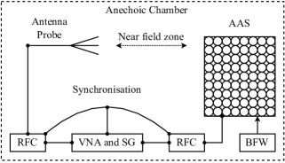
Figure 1: $S_{12}/S_{21}$ – parameter measurement setup.

In the sequel, we assume that measurements are made within an anechoic chamber without external interference sources and that the internal non-linear distortions (intermodulation components) are corrected by their respective algorithms (e.g. DPD, PIMC). Therefore, the resulting beam pattern is only affected by frequency-selective linear multiplicative effects applied at each RF channel feeding to its antenna – $z_{f}$ and imperfections of an array itself – $g_{f}$. In practice, such distortions depend on the temperature and dynamics caused by hardware degradations, which in this study are assumed to be static (memoryless). The effects of $v_{f}$ and $g_{f}$ on the BFW are shown in Fig. 2, and are defined as:

$$w^{d}_{f,n}=w_{f,n}\cdot v_{f,n}\cdot g_{f,n};\ \ \ w,w^{d},v,g\in\mathbb{C},$$ (2)

where $f$ denotes the operating frequency point or a sub-carrier within a bandwidth, $n$ denotes antenna number, while $w_{f,n}$ and $w^{d}_{f,n}$ denote the desired and distorted BFW respectively. Note that the set of $w^{d}_{f,n}$ values is obtained directly from the measured $S_{12}$ or $S_{21}$ parameters. The AAS under test supports two beamforming modes: DBF and emulated ABF. In the latter case, each antenna element is assigned adjustable discrete phase and amplitude values, which are “unique” for the whole operating bandwidth.

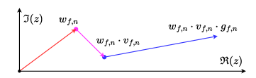
Figure 2: Distortion of a single beamforming weight into a non-calibrated state. Only the resulting vectors are shown.

The effects of distortion can be further visualised in the following example. Consider an ABF system with 64 radiating elements and $5$-bit precision, which allows for 32 gain values and 32 phase states resulting in 1024 complex-valued $w_{f,n}$, to choose from for each antenna. As shown in Fig. 3a, $w_{f,n}$ (red stars) can be allocated across available domain (black dots). Although discretisation in ABF negatively affects the radiation patterns, an appropriate increase in the precision range allows to reach the desired DBF quality. Once the studied distortion is induced, as shown in Fig. 3b and Fig. 3c, the resulting $w^{d}_{f,n}$ weights no longer correspond to the BFW that were assumed during the beamforming synthesis of $w_{f,n}$.

This observation gives rise to our first question: how to perform AAS calibration, while satisfying an extensive set of technical constraints?

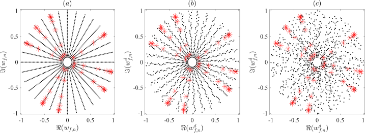
Figure 3: (a) – $w_{f,n}$ unaffected by distortion. (b) – small-scale distortion. (c) large-scale distortion. Black dots – available ABF weights. Red stars – subset chosen for ABF. Each channel has its own distortion pattern.

IV Calibration as High-Dimensional Regression

To answer the first question, we have to look at calibration with a scanning probe [12]. By design, it is used to create a set of initial conditions for mutual coupling and other calibration methods. The probe connected to the measurement hardware is placed in front of an active antenna element of the AAS, while others are in inactive states. Scattering parameters are measured, and the estimated frequency responses are stored in a static look-up table (LUT). These measurements reliably capture all necessary information to model the behaviour of RF imperfections for the purposes of array calibration. However, the scale of massive MIMO systems, the number of discrete BFW in ABF cases, combined with complex test setup and unsupported continuous calibration, make such a direct approach unfeasible. This leads to our second question: how to build upon “LUT” calibration to satisfy modern constraints?

Problem Formulation.

We consider that $S_{12}/S_{21}$ measurements form a function space $f$ (Fig. 4a), such that $f:\mathcal{F}\times\mathcal{N}\times\mathcal{Z}\rightarrow\mathcal{Y}$, where $\mathcal{F},\mathcal{N}\in\mathbb{R}$ are domains of continuous and discrete values corresponding to operating frequencies and RF channel numbers, respectively. $\mathcal{Z},\mathcal{Y}\in\mathbb{C}$ are continuous (for DBF) or discrete (for ABF) domains of undistorted and distorted BFW. Assuming significant sparsity or irregularity of measurements, our problem becomes one of a functional approximation. In other words, we address a problem of non-linear regression, where given $M$ evaluations $y=\left\{\mathbf{x}_{m},f\left(\mathbf{x}_{m}\right)\right\}_{m=1}^{M}$, we want to recover the underlying function. Once recovered, it can be used for AAS calibration, thus remedying the main disadvantage of conventional “probe calibration” methodology. In addition, three assumptions need to be noted with regard to the regression setting. First, measurements with corresponding BFW are $\mathbb{C}$–valued, so in order to simplify the problem, we solve the regression for $\Re(z)$ and $\Im(z)$ domains, separately. This widens the range of applicable regression models. Second, by treating $\mathcal{N}$ as a continuous domain, our functional space is assumed to be smooth. Third, we assume that the underlying RF impairments are static, in a sense that measurements do not contain changepoints and the system does not undergo a distribution shift. Thus, our third question is: which data-driven model can satisfy the criteria of sample efficiency, robustness and convergence guarantees?

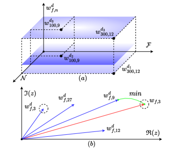
Figure 4: (a) – Function space, derived from $S_{12}/S_{21}$ measurements. (b) – Calibration procedure in ABF systems based on Euclidean distances between $w_{f,n}$ and $w_{f,n}^{d}$.

V AAS Calibration via Gaussian Process Models

Based on the above considerations, our goal is to approximate and interpolate an underlying function in a data-driven fashion. A wide range of candidate methods includes polynomial regression, splines, reproducing kernel Hilbert spaces and DNN. However, they only provide deterministic error bounds, and the latter relies on large datasets. Moreover, our data can be very sparse, which renders deterministic models undesirable. The alternative that satisfies all our requirements is a GP regression which belongs to a class of Bayesian non-parametric models [13], and represents an unknown function $f(\mathbf{x})$ by a realization sampled from a stochastic process with corresponding stochastic error bounds and convergence guarantees [14, 15]. Before proceeding with AAS calibration solution, we first provide necessary prerequisites for GPs.

Gaussian Process Regression.

GPs define a distribution over functions, such that any finite collection of random variables $f$ has a joint Gaussian distribution (3)

$$f(\mathbf{x})=\left[f\left(\mathbf{x}_{1}\right),\ldots,f\left(\mathbf{x}_{m}\right)\right]^{\top}\sim\mathcal{N}(\boldsymbol{\mu},k).$$ (3)

Our dataset $\mathcal{D}$ consists of test input vectors $\mathbf{x}^{*}$ and noisy samples $\mathbf{y}=\{y_{1}\left(\mathbf{x}_{1}\right),\dots,y_{m}\left(\mathbf{x}_{m}\right)\}$, corrupted by Gaussian noise $\varepsilon_{i}\sim\mathcal{N}\left(0,\sigma_{\text{noise }}^{2}\right),i=1,2,\ldots,m$, that are observed at $\mathbf{x}=\{\mathbf{x}_{1},\dots,\mathbf{x}_{m}\}$, respectively. Modelling properties of a GP are determined by its mean $\boldsymbol{\mu}$ (assumed $\boldsymbol{\mu}=0$) and covariance kernel function $k\left(\mathbf{x},\mathbf{x}^{\prime}\right)$. In the resulting model (4), the prior and measurement models are Gaussian, leading to a Gaussian posterior and a learning problem that amounts to the computation of the conditional mean $\mathbb{E}\left[f\left(\mathbf{x}^{*}\right)\right]$ and covariances $\mathbb{V}\left[f\left(\mathbf{x}^{*}\right)\right]$ (5) of the process at $\mathbf{x}^{*}$ in closed forms:

$$f(\mathbf{x})\sim\mathcal{GP}\left(\boldsymbol{\mu},k\left(\mathbf{x},\mathbf{x}^{\prime}\right)\right)\ \ y_{i}=f\left(\mathbf{x}_{i}\right)+\varepsilon_{i},$$ (4)

$$\begin{gathered}\mathbb{E}\left[f\left(\mathbf{x}^{*}\right)\right]=\mathbf{k}^{*\top}\left(\mathbf{K}+\sigma_{\text{noise }}^{2}\mathbf{I}_{m}\right)^{-1}\mathbf{y},\\ \mathbb{V}\left[f\left(\mathbf{x}^{*}\right)\right]=k\left(\mathbf{x}^{*},\mathbf{x}^{*}\right)-\mathbf{k}^{*\top}\left(\mathbf{K}+\sigma_{\text{noise }}^{2}\mathbf{I}_{m}\right)^{-1}\mathbf{k}^{*},\end{gathered}$$ (5)

where $\mathbf{K}_{i,j}=k\left(\mathbf{x}_{i},\mathbf{x}_{j}\right)$ is $m\times m$ positive semi-definite covariance matrix, $\mathbf{k}^{*}$ is a $m$–dimensional vector with each entry being $k\left(\mathbf{x}^{*},\mathbf{x}_{i}\right)$. With (5), the learning process is formally defined as (6) [13]

$$p\left(f\left(\mathbf{x}^{*}\right)\mid\mathcal{D}\right)=\mathcal{N}\left(f\left(\mathbf{x}^{*}\right)\mid\mathbb{E}\left[f\left(\mathbf{x}^{*}\right)\right],\mathbb{V}\left[f\left(\mathbf{x}^{*}\right)\right]\right).$$ (6)

The generalisation and functional properties (e.g. smoothness, periodicity, non-linearity) of GPs are encoded by covariance kernels and their hyperparameters $\theta$, which can be optimised by maximizing the marginal likelihood of the data, conditioned on $\theta$ and $\mathbf{x}$. An example of a commonly used covariance is a rational quadratic (RQ) kernel, (7) where $\theta$ includes length-scale $\ell$, magnitude $\sigma^{2}$ and $\alpha$ that determines the relative weighting of the large-scale and small-scale variations:

$$k_{\mathrm{RQ}}\left(\mathbf{x},\mathbf{x}^{\prime}\right)=\sigma^{2}\left(1+\left({\left(\mathbf{x}-\mathbf{x}^{\prime}\right)^{2}}/{2\alpha\ell^{2}}\right)\right)^{-\alpha}.$$ (7)

Kronecker Extension.

In order to support regression over a three-dimensional setting, we apply fast scalable Kronecker inference, originally proposed by Flaxman et al. in [16]. The combination of GPs and Kronecker methods relies on the assumption that the kernel in the former is a product of kernels applied across input dimensions allocated on the Cartesian product grid, without constraints on the grid’s regularity and equal cardinality of its axis. This principle allows to decompose the covariance matrix $\mathbf{K}$ into a Kronecker product $\mathbf{K}=\mathbf{K}_{1}\otimes\dots\otimes\mathbf{K}_{D}$. Kronecker methods are extended in [16] by utilising the Laplace approximation to model the posterior distribution of the GP [13], while also involving the linear conjugate gradients for inference and a lower bound on the GP marginal likelihood for kernel learning. Moreover, their runtime and storage complexities are $\mathcal{O}\left(Dm^{\frac{D+1}{D}}\right)$ and $\mathcal{O}\left(Dm^{\frac{2}{D}}\right)$, for $D$ input dimensions with $m$ data points, which makes them advantageous for efficient learning and implementation.

Calibration Procedure.

We partition the AAS calibration task into two parts. The first part consists of creating a sparse measurement dataset $\mathcal{D}$ over a three-dimensional uniform grid $\mathcal{F}\times\mathcal{N}\times\mathcal{Z}$, where each entry $w_{f,n}^{d}$ is converted from $S_{12}/S_{21}$. Here we assume that a single measurement captures the full operating bandwidth. Next, the $\Re(w)$ and $\Im(w)$ components are approximated separately by two GP models. In the second part, the learnt models are deployed at the AAS and sampled each time the BFWs change. For DBF systems, the BFW are adjusted in accordance with conventional methods that rely on near-field measurements. In the case of ABF, the situation is different, since the BFWs are chosen from a discrete set. In our scheme, information about the distortion of this set is obtained by surrogate measurements sampled from a GP model. Thus, the task of ABF calibration is to choose $w_{f,n}^{d}$ closest to the current $w_{f,n}$ based on Euclidean distances (Fig. 4b) or, alternatively, to choose the set $w_{f,n}^{d}$ that best describes the ratios between $w_{f,n}$, such as ${w_{f,1}}/{w_{f,2}}\dots w_{f,n}/{w_{f,n-1}}$.

VI Simulation Results

We model $\Re(w^{d})$ and $\Im(w^{d})$ components of RF impairments as a set of smooth functions $f(\mathcal{F},\mathcal{N})$ defined by a finite Fourier series with random coefficients [17]. Where total number of functions is determined by a range of BFW in AAS and, in case of ABF, discretisation precision. In our experiments, GP models utilise a Kronecker product of two RQ and one spectral mixture kernels, with parameters optimised according to [16].

As an example, in Fig. 5 we show impairment surfaces and their GP approximations, for a ABF with $\mathcal{N}=1024$, $\mathcal{F}=400$ MHz (with granularity of $1$ MHz) and 1024 BFW $w_{f,n}$. For the purpose of visual clarity, we show a “slice” of impairment space, corresponding to a single $w_{f,n}$ out of $1024$. Left half of subplots shows ground-truth surfaces of $\Re(w_{f,n}^{d})$ and $\Im(w_{f,n}^{d})$ values. While right half – results of GP modelling based on randomly sampled $w_{f,n}^{d}$ observations. We compare the original and restored surfaces according to the normalised RMSE criterion averaged across a series of $5\times 10^{4}$ random $w_{f,n}^{d}$ space-realisations, in which models utilising $5,10,15\text{ and }20\%$ of all possible measurements of $w_{f,n}^{d}$ were compared. With proposed approach best approximation quality was achieved for $15\%$ and $20\%$ utilisation, with an averaged RMSE of $2.3710e^{-04}$ and $1.0380e^{-04}$ respectively.

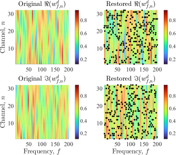
Figure 5: Slices of $w^{d}$ space for 32 $\times$ 32 antenna array and 400 MHz operating bandwidth. Colours indicate magnitude and black dots – locations of observed samples for GP modelling.

After restoring $w_{f,n}^{d}$ with the GP models, we study the performance of AAS calibration in both ABF and DBF at different scales. In all cases, the AAS use rectangular arrays with uniform element spacing of $0.5\lambda$ and GPs with an approximation RMSE lower than $10^{-3}$. All beam patterns, depicted below, show the azimuth $\phi^{\circ}$ and elevation $\theta^{\circ}$ cuts in the center of the operating bandwidth of 400 MHz and share the same notation. The desired beam patterns (based on $w_{f,n}$) are depicted by black curves, the distorted ones (based on $w_{f,n}^{d}$) by blue curves and the calibrated ones (based on knowledge of the restored $w_{f,n}^{d}$) by dashed red curves. The BFW are synthesised using convex optimisation with constraints on angular positions of UE (magenta dots) and interference sources (black dots).

Continuing the ABF case with 1024 $w_{f,n}$, we show calibration performance for ABF systems with 1024 and 4096 antenna elements, with the latter shown in Fig. 6. In both scenarios the BPA RMSE improvement ratio was significantly hindered by unavoidable discretisation of BFW, resulting only in $BPA^{ABF}/BPA_{calib.}^{ABF}=2.23$ and $1.91$ respectively. Lastly, we switch to DBF arrays with $64\times 64$ (Fig. 7) and $128\times 128$ (Fig. 8) elements, where in the same experiment setting $BPA^{DBF}/BPA_{calib.}^{DBF}$ achieves values of $8.11$ and $10.04$.

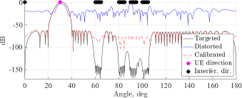
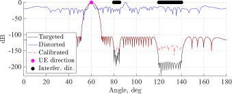
Figure 6: ABF with $64\times 64$ element array; UE $\phi^{\circ},\theta^{\circ}=(30;60)$; interference sets: $\phi^{\circ}=[60^{\circ},65^{\circ}],...,[100^{\circ},105^{\circ}]$ and $\theta^{\circ}=[80^{\circ},85^{\circ}],[120^{\circ},140^{\circ}]$.

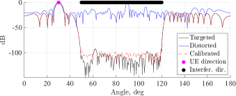
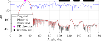
Figure 7: DBF with $64\times 64$ element array; UE $\phi^{\circ},\theta^{\circ}=(30;30)$; interference sets: $\phi^{\circ}=[50^{\circ},120^{\circ}]$ and $\theta^{\circ}=[100^{\circ},120^{\circ}],...,[150^{\circ},170^{\circ}]$.

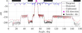
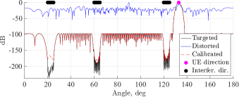
Figure 8: DBF with $128\times 128$ element array; UE $\phi^{\circ},\theta^{\circ}=(70;133)$; interference sets $\phi^{\circ}=[10^{\circ},30^{\circ}],...,[165^{\circ},180^{\circ}]$ and $\theta^{\circ}=[20^{\circ},25^{\circ}],...,[120^{\circ},125^{\circ}]$.

VII Conclusions and Future Work

In this work, we have proposed a novel approach to AAS calibration based on the intersection of near-field measurement methodologies and Bayesian modelling. Our solution captures the complete set of internal and external RF hardware impairments via a sparse set of precise near-field $S_{12}/S_{21}$ parameter measurements and restores the rest via high-dimensional GP regression models. Once deployed at an operating AAS, the latter actively adjusts the beamforming parameters in accordance with the learnt impairment values and thus results in corrected beam patterns and a consequential performance improvement of algorithms that rely on their high fidelity. Furthermore, it avoids the drawbacks of conventional methods, such as relying on RF hardware constraints or standardised communication protocols and signal formats.

Based on the obtained results and the modelling properties of GPs, we envision a future work in the context of three key directions: extending the solution to HBF architectures, modelling of RF impairments with temporal dynamics related to temperature drifts or hardware degradation and lastly, incorporating uncertainty quantification into the calibration process. Finally, as we continue the line of thought about algorithm design and evaluation, we argue that the domain of AAS calibration would benefit from a unified benchmarking test and performance metric that will allow researchers to analyse the properties of their proposals in an unbiased and consistent way.

References

- [1] Y. Wu, Y. Gu, and Z. Wang, “Efficient Channel Estimation for mmWave MIMO With Transceiver Hardware Impairments,” IEEE Transactions on Vehicular Technology, vol. 68, no. 10, pp. 9883–9895, Oct. 2019.
- [2] G. Tian, H. Tataria, and F. Tufvesson, “Amplitude and Phase Estimation for Absolute Calibration of Massive MIMO Front-Ends,” in ICC 2020 - 2020 IEEE International Conference on Communications (ICC), Jun. 2020, pp. 1–7.
- [3] R. Nie, L. Chen, N. Zhao, Y. Chen, W. Wang, and X. Wang, “Impact and Calibration of Nonlinear Reciprocity Mismatch in Massive MIMO Systems,” IEEE Transactions on Wireless Communications, vol. 20, no. 10, pp. 6418–6435, Oct. 2021.
- [4] X. Luo, F. Yang, and H. Zhu, “Massive MIMO Self-Calibration: Optimal Interconnection for Full Calibration,” IEEE Transactions on Vehicular Technology, vol. 68, no. 11, pp. 10 357–10 371, Nov. 2019.
- [5] X. Wei, Y. Jiang, Q. Liu, and X. Wang, “Calibration of Phase Shifter Network for Hybrid Beamforming in mmWave Massive MIMO Systems,” IEEE Transactions on Signal Processing, vol. 68, pp. 2302–2315, 2020.
- [6] Y. Aoki, Y. Kim, Y. Hwang, H. Kang, S. Kim, A.-S. Ryu, and S.-G. Yang, “An Intermodulation Distortion Oriented 256-Element Phased-Array Calibration for 5G Base Station,” in 2022 IEEE/MTT-S International Microwave Symposium - IMS 2022, Jun. 2022, pp. 518–521.
- [7] T. Iye, P. van Wyk, T. Matsumoto, Y. Susukida, S. Takaya, and Y. Fujii, “Neural Network-Based Phase Estimation for Antenna Array Using Radiation Power Pattern,” IEEE Antennas and Wireless Propagation Letters, vol. 21, no. 7, pp. 1348–1352, Jul. 2022.
- [8] T. Moon, J. Gaun, and H. Hassanieh, “Know Your Channel First, then Calibrate Your mmWave Phased Array,” IEEE Design & Test, vol. 37, no. 4, pp. 42–51, Aug. 2020.
- [9] M. Willerton and A. Manikas, “Array shape calibration using a single multi-carrier pilot,” in Sensor Signal Processing for Defence (SSPD 2011), Sep. 2011, pp. 1–6.
- [10] K. Wang, J. Yi, F. Cheng, Y. Rao, and X. Wan, “Array Errors and Antenna Element Patterns Calibration Based on Uniform Circular Array,” IEEE Antennas and Wireless Propagation Letters, vol. 20, no. 6, pp. 1063–1067, Jun. 2021.
- [11] C. Shan, X. Chen, H. Yin, W. Wang, G. Wei, and Y. Zhang, “Diagnosis of Calibration State for Massive Antenna Array via Deep Learning,” IEEE Wireless Communications Letters, vol. 8, no. 5, pp. 1431–1434, Oct. 2019.
- [12] I. Şeker, “Calibration methods for phased array radars,” in Radar Sensor Technology XVII, vol. 8714. SPIE, May 2013, pp. 294–308.
- [13] C. E. Rasmussen and C. K. I. Williams, Gaussian Processes for Machine Learning. Cambridge, Mass: The MIT Press, Nov. 2005.
- [14] A. L. Teckentrup, “Convergence of Gaussian Process Regression with Estimated Hyper-Parameters and Applications in Bayesian Inverse Problems,” SIAM/ASA J. Uncertainty Quantification, vol. 8, no. 4, pp. 1310–1337, Jan. 2020.
- [15] G. Wynne, F.-X. Briol, and M. Girolami, “Convergence guarantees for Gaussian process means with misspecified likelihoods and smoothness,” J. Mach. Learn. Res., vol. 22, no. 1, pp. 123:5468–123:5507, Jul. 2022.
- [16] S. Flaxman, A. Wilson, D. Neill, H. Nickisch, and A. Smola, “Fast Kronecker Inference in Gaussian Processes with non-Gaussian Likelihoods,” in Proceedings of the 32nd International Conference on Machine Learning. PMLR, Jun. 2015, pp. 607–616.
- [17] S. Filip, A. Javeed, and L. N. Trefethen, “Smooth Random Functions, Random ODEs, and Gaussian Processes,” SIAM Rev., vol. 61, no. 1, pp. 185–205, Jan. 2019.