Causal Recurrent Variational Autoencoder for Medical Time Series Generation

Abstract

We propose causal recurrent variational autoencoder (CR-VAE), a novel generative model that is able to learn a Granger causal graph from a multivariate time series $\mathbf{x}$ and incorporates the underlying causal mechanism into its data generation process. Distinct to the classical recurrent VAEs, our CR-VAE uses a multi-head decoder, in which the $p$-th head is responsible for generating the $p$-th dimension of $\mathbf{x}$ (i.e., $\mathbf{x}^{p}$). By imposing a sparsity-inducing penalty on the weights (of the decoder) and encouraging specific sets of weights to be zero, our CR-VAE learns a sparse adjacency matrix that encodes causal relations between all pairs of variables. Thanks to this causal matrix, our decoder strictly obeys the underlying principles of Granger causality, thereby making the data generating process transparent. We develop a two-stage approach to train the overall objective. Empirically, we evaluate the behavior of our model in synthetic data and two real-world human brain datasets involving, respectively, the electroencephalography (EEG) signals and the functional magnetic resonance imaging (fMRI) data. Our model consistently outperforms state-of-the-art time series generative models both qualitatively and quantitatively. Moreover, it also discovers a faithful causal graph with similar or improved accuracy over existing Granger causality-based causal inference methods. Code of CR-VAE is publicly available at https://github.com/hongmingli1995/CR-VAE.

Introduction

Multivariate time series data are ubiquitous in numerous real-world applications. e.g., the electroencephalogram (EEG) signals (Isaksson, Wennberg, and Zetterberg 1981), the climate records (Runge et al. 2019), and the stellar light curves in astronomy (Huijse et al. 2012). Traditional machine learning tasks on time series data include anomaly detection, segmentation, forecasting, classification, etc. Among them, the time series forecasting or prediction, which uses past or historical observations to predict future values, is perhaps the most popular one.

In recent years, the design of generative models for time series data emerged as a challenge. One reason is that most of existing machine learning models, especially deep neural networks, are data-hungry, which means that a sufficient number of (labeled) samples are required during training before their practical deployment. Unfortunately, in some sensitive applications, especially those involving medical and healthcare domains, collecting and exchanging real data from patients requires a long administrative process or is even prohibited. This in turn may inhibit research progress on model comparison and reproducibility.

A good generative model for time series is expected to model both the joint distribution $p(\mathbf{x}_{1:T})$ and the transition dynamics $p(\mathbf{x}_{t}|\mathbf{x}_{1:t-1})$ for any $t$. Although most of popular predictive models, such as autoregressive integrated moving average (ARIMA), kernel adaptive filters (KAF) (Liu, Pokharel, and Principe 2008) and deep state-space models (SSMs) (Rangapuram et al. 2018), provide different ways to capture $p(\mathbf{x}_{t}|\mathbf{x}_{1:t-1})$ or $p(\mathbf{x}_{t}|\mathbf{x}_{t-\tau:t-1})$ in the window of length $\tau$, they are deterministic mappers, rather than generative. In other words, these models are incapable of inferring unobserved latent factors (such as trend and seasonality) from observational data, and generating new time series values by sampling from a tractable latent distribution.

On the other hand, causal inference from time series data has also attracted increasing attention. Taking the functional magnetic resonance imaging (fMRI) data as an example, it is of paramount importance to identify causal influences between brain activated regions (Deshpande et al. 2009). This causal graph may also provide insights into brain network-based psychiatric disorder diagnosis (Wang et al. 2020).

Given the urgent need for a reliable time series generative model and the modern trend of causal inference, one question arises naturally: can we develop a new generative model for time series such that it can also be used for causal discovery? In this paper, we give an explicit answer to this question. To this end, we develop causal recurrent variational autoencoder (CR-VAE), which, to the best of our knowledge, is the first endeavor to integrate the concept of Granger causality within a recurrent VAE framework. Specifically, given a $M$-variate time series $\mathbf{x}=(\mathbf{x}^{1},\mathbf{x}^{2},\cdots,\mathbf{x}^{M})$, our CR-VAE consists of an encoder and a multi-head decoder, in which the $p$-th head is responsible for generating the $p$-th dimension of $\mathbf{x}$ (i.e., $\mathbf{x}^{p}$). We impose a sparsity penalty on the weight matrix that connects input and hidden state (in the decoder), thereby encouraging the model to learn a sparse matrix $A\in\mathbb{R}^{M\times M}$ to encode the Granger causality between pairwise dimensions of $\mathbf{x}$. Such design also makes the generation process compatible with the underlying principles of Granger causality (i.e., causes appear prior to effects). Additionally, we also propose an error-compensation module to take into account the instantaneous influence $\varepsilon_{t}$ excluding the past of one process.

We conduct extensive experiments on synthetic sequences and real-world medical time series. In terms of time series generation, we evaluate the closeness between real data distribution and synthetic data distribution both qualitatively and quantitatively. In terms of causal discovery, we compare our discovered causal graph with state-of-the-art (SOTA) approaches that also aim to identify the Granger causality. Our model achieves competitive performance in both tasks.

Background Knowledge

The proposed work lies at the intersection of multiple strands of research, combining themes from autoregressive models for temporal dynamics, Granger causality for causal discovery, and VAE-based time series models.

Time Series Generative Models

A deep generative model $g_{\theta}$ is trained to map samples from a simple and tractable distribution $p(\mathbf{z})$ to a more complicated distribution $p(g_{\theta}(\mathbf{z}))$, which is similar to the true distribution $p(\mathbf{x})$. For time series data, one can simply generate synthetic time series under a Generative Adversarial Network (GAN) (Goodfellow et al. 2014) framework, by making use recurrent neural networks in both the generator and the discriminator (Mogren 2016; Esteban, Hyland, and Rätsch 2017; Takahashi, Chen, and Tanaka-Ishii 2019). However, these GAN-based approaches only model the joint distribution $p(\mathbf{x}_{1:T})$, but fails to take the transaction dynamics $p(\mathbf{x}_{t}|\mathbf{x}_{1:t-1})$ into account. TimeGAN (Yoon, Jarrett, and Van der Schaar 2019) addresses this issue by estimating and training this conditional density in an internal latent space.

Apart from a few early efforts (e.g., (Fabius and Van Amersfoort 2014)), the VAE-based time series generator is less investigated. Some of them, such as Z-forcing (Goyal et al. 2017)), even encode the future information in the autoregressive structure, thereby violating the underlying principles of Granger causality (Granger 1969) that cause happens prior to its effect. The recently developed TimeVAE (Desai et al. 2021) uses convolutional neural networks in both encoder and decoder, and adds a few parallel blocks in the decoder where each block accounts for a specific temporal property such as trend and seasonality. However, the building blocks introduce a set of new hyper-parameters which are hard to determine in practice.

In this work, we also develop a new VAE-based time series generative model. Compared to the above mentioned approaches, our distinct properties include: 1) the ability to discover Granger causality, which makes the model itself more transparent than other baselines; 2) the ability to explicitly model conditional density $p(\mathbf{x}_{t}|\mathbf{x}_{1:t-1})$; and 3) a rigorous guarantee on the generation process to obey the underlying principles of Granger causality.

Causal Discovery of Time Series

Substantial efforts have been made on the causal discovery of a $M$-variate time series $\mathbf{x}=(\mathbf{x}^{1},\mathbf{x}^{2},\cdots,\mathbf{x}^{M})$, where the goal is to discover, from the observational data, the causal relations between different dimensions of data in different time instants, e.g., if $\mathbf{x}^{p}$ causes $\mathbf{x}^{q}$ in time $t$ with a lag $\tau$?

Different types of causal graphs can be considered for time series (Assaad, Devijver, and Gaussier 2022b). Here, we consider recovery of a Granger causal graph, which separates past observations and present values of each variable and aims to discover all possible causations from past to present. Formally, the Graph causal graph is defined as:

Definition (Granger Causal Graph).

Let $\mathbf{x}=(\mathbf{x}^{1},\mathbf{x}^{2},\cdots,\mathbf{x}^{M})$ be a $M$-dimensional time series of length $T$, where, for time instant $t$, each $\mathbf{x}_{t}$ is a vector $\mathbf{x}_{t}=[\mathbf{x}_{t}^{1},\mathbf{x}_{t}^{2},\cdots,\mathbf{x}_{t}^{M}]$ in which $\mathbf{x}_{t}^{p}$ represents a measurement of the $p$-th time series at time $t$. Let $G=(V,E)$ the associated Granger causal graph with $V$ representing the set of nodes and $E$ the set of edges. The set $V$ consists of the set of $M$ dependent time series $\mathbf{x}^{1},\mathbf{x}^{2},\cdots,\mathbf{x}^{M}$. There is an edge connects node $\mathbf{x}^{p}$ to $\mathbf{x}^{q}$ if: 1) for $p\neq q$, the past values of $\mathbf{x}^{p}$ (denoted $\mathbf{x}_{t-}^{p}$) provide unique, statistically significant information about the prediction of $\mathbf{x}_{t}^{q}$; and 2) for $p=q$, $\mathbf{x}_{t-}^{q}$ causes $\mathbf{x}_{t}^{q}$ (i.e., self-cause).

Note that, the Granger causal graph may have self-loops as the past observations of one time series always cause its own present value. Hence, it does not need to be acyclic.

The approaches on causal discovery of time series are diverse. Interested readers can refer to (Assaad, Devijver, and Gaussier 2022b) for a comprehensive survey. In the following, we briefly introduce the basic idea of Granger causality (Granger 1969) and its recent advances.

Wiener was the first mathematician to introduce the notion of “causation” in time series (Wiener 1956). According to Wiener, the time series or variable $\mathbf{x}$ causes another variable $\mathbf{y}$ if, in a statistical sense, the prediction of $\mathbf{y}$ is improved by incorporating information about $\mathbf{x}$. However, Wiener’s idea was not fully developed until $1969$ by Granger (Granger 1969), who defined the causality in the context of linear multivariate auto-regression (MVAR) by comparing the variances of the residual errors with and without considering $\mathbf{x}$ in the prediction of $\mathbf{y}$. Not surprisingly, the basic idea of Granger causality can be extended to non-linear scenario by the kernel trick (Marinazzo, Pellicoro, and Stramaglia 2008) or by fitting locally linear models in the reconstructed phase space (Chen et al. 2004). The deep neural networks have been leveraged recently to identify Granger causality. Neural Granger causality (Tank et al. 2021) is the first method that learns the causal graph by introducing sparsity constraints on the weights of autoregressive networks. The Temporal Causal Discovery Framework (TCDF) (Nauta, Bucur, and Seifert 2019) uses an attention mechanism within dilated depthwise convolutional networks to learn complex non-linear causal relations and, in special cases, hidden common causes.

Information-theoretic measures, such as directed information (Massey 1990) and transfer entropy (TE) (Schreiber 2000), provide an alternative model-free approach to quantify the directed information flow among stochastic processes. Specifically, TE is defined as the conditional mutual information $I(\mathbf{y}_{t};\mathbf{x}_{t-}|\mathbf{y}_{t-})$. However, TE is incapable to quantify instantaneous causality (Amblard and Michel 2012) and notoriously hard to estimate, especially in high-dimensional space. Recently, (De La Pava Panche, Alvarez-Meza, and Orozco-Gutierrez 2019) relies on the matrix-based Rényi’s $\alpha$-order entropy (Giraldo, Rao, and Principe 2014) to estimate TE and achieves compelling performances. Interestingly, TE is equivalent to Granger causality in MVAR for Gaussian variables (Barnett, Barrett, and Seth 2009). Essentially, both definitions can be regarded as comparing the model with and without considering the intervening variable $\mathbf{y}$ (Chen, Feng, and Lu 2021).

We provide in the supplementary material a table of other related works with additional details. Note, however, that none of the mentioned causal inference approaches can be used for time series generation.

Causal Recurrent Variational Autoencoder

Problem Formulation and Objectives

Our high-level objective is to learn a distribution $\hat{p}(\mathbf{x}_{1:T})$ that matches well the true joint distribution $p(\mathbf{x}_{1:T})$. From a generative model perspective, this is achieved by sampling from a simple and tractable distribution $p(\mathbf{z})$ and then map to a more complicated distribution $\hat{p}(\mathbf{x}_{1:T})$. Usually, it is difficult to model $p(\mathbf{x}_{1:T})$ depending on its dimension $M$, length $T$ and possibly non-stationary nature. To this end, we can apply the autoregressive decomposition $p(\mathbf{x}_{1:T})=\prod^{T}_{t=1}p(\mathbf{x}_{t}\mid\mathbf{x}_{1:t-1})$ to infer the sequence iteratively (West and Harrison 2006). The objective reduces to learn a conditional density $\hat{p}(\mathbf{x}_{t}\mid\mathbf{x}_{1:t-1})$ that equals to the true density $p(\mathbf{x}_{t}\mid\mathbf{x}_{1:t-1})$. Hence, our first objective is:

$$\min_{\hat{p}}\mathcal{D}(p(\mathbf{x}_{t}\mid\mathbf{x}_{1:t-1})||\hat{p}(\mathbf{x}_{t}\mid\mathbf{x}_{1:t-1})),$$ (1)

for any $t$, where $\mathcal{D}$ is the divergence between distributions.

Our second objective is straightforward. Suppose $\mathbf{x}^{1},\mathbf{x}^{2},\cdots,\mathbf{x}^{M}$ are intrinsically correlated by a Granger causal graph $G=(V,E)$, we can characterize $G$ by its (unweighted) adjacency matrix $A$, whose $(u,v)$-th entry is defined as:

$$A_{u,v}=\begin{cases}1&\text{$\mathbf{x}_{t-}^{v}$ causes $\mathbf{x}_{t}^{u}$; i.e., edge $(u,v)\in E$}\\ 0&\text{otherwise}.\end{cases}$$ (2)

Now, let $\text{PA}(\mathbf{x}^{p})$ denote the set of parents (or causes) of $\mathbf{x}^{p}$ in $G$ (i.e., the non-zero elements in the $p$-th row of $A$), motivated by the additive noise model with nonlinear functions (Hoyer et al. 2008; Chu, Glymour, and Ridgeway 2008), we can represent $\mathbf{x}_{t}^{p}$ as follows:

$$\mathbf{x}_{t}^{p}=f_{p}\left(\mathbf{x}_{t-}^{p},\text{PA}(\mathbf{x}^{p})_{t-}\right)+\varepsilon_{t}^{p},$$ (3)

in which $\mathbf{x}_{t-}^{p}$ denotes past observations of $\mathbf{x}_{t}^{p}$, $\text{PA}(\mathbf{x}^{p})_{t-}$ denotes past observations of cause variables of $\mathbf{x}^{p}$, $\varepsilon_{t}^{p}$ are jointly independent over $p$ and $t$ and, for each $p$, i.i.d., in $t$.

Therefore, our second objective is to learn $f_{p}$ for each $\mathbf{x}^{p}$ and infer the matrix $A$.

Methodology

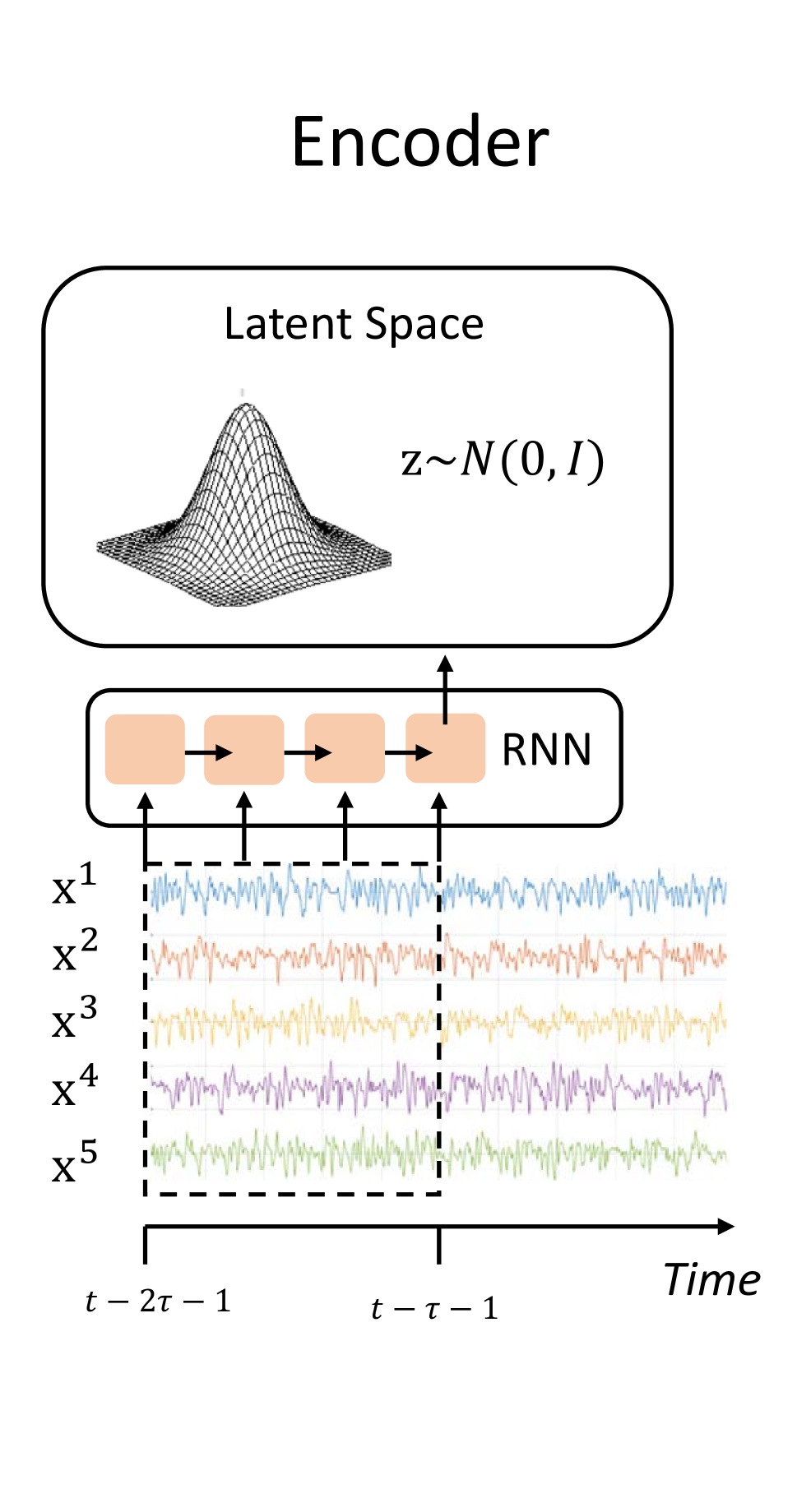
(a) The CR-VAE encoder approximates the intractable posterior $p(\mathbf{z}|\mathbf{x})$. We extract a time segment $\mathbf{x}_{t-2\tau-1:t}$ as our training data, and and use the first half clip $\mathbf{x}_{t-2\tau-1:t-\tau-1}$ as the input to encoder.

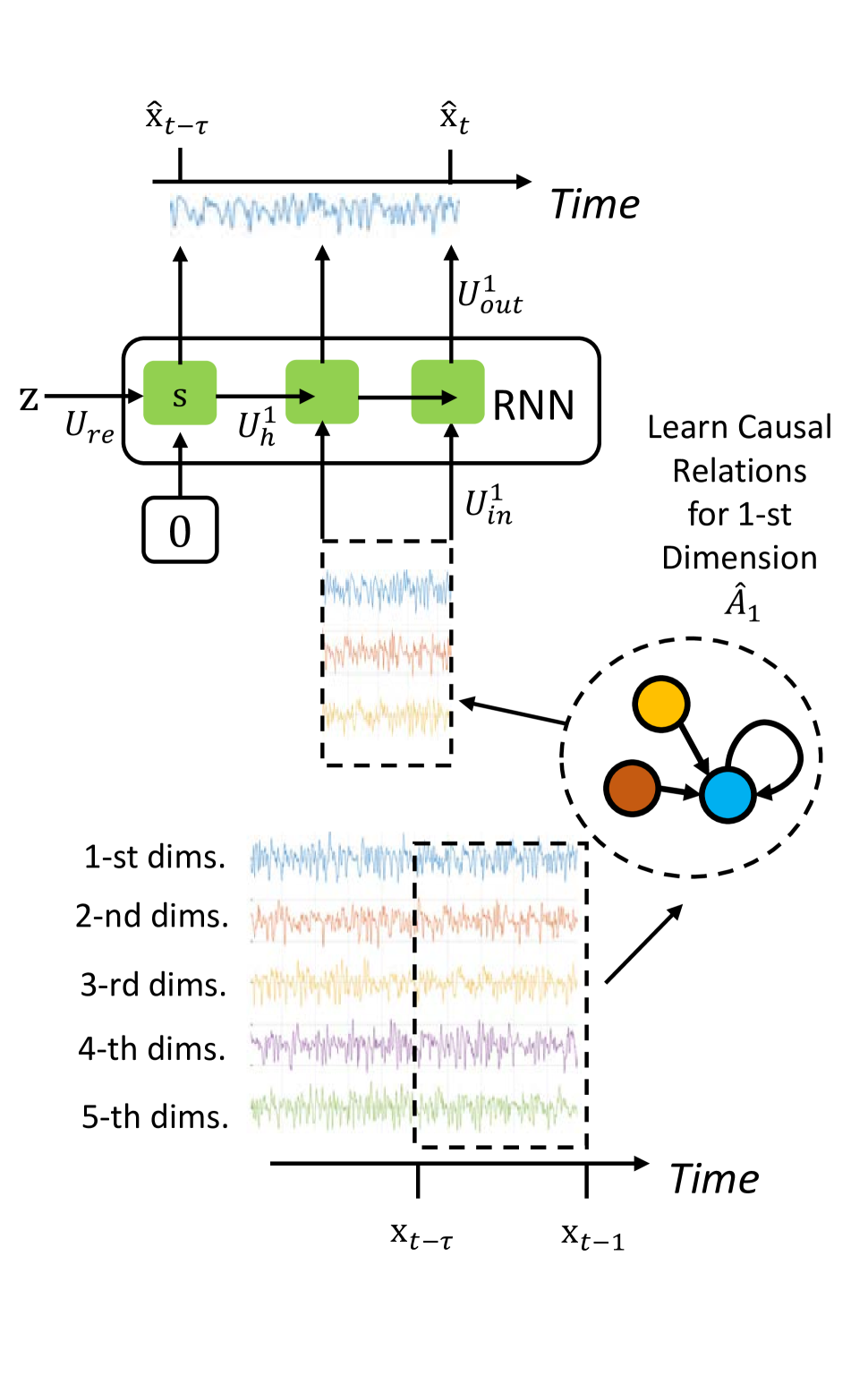
(b) The first head of the decoder, which predicts the 1-st dimension of $\mathbf{x}$. The second half of the time clip is used as the decoder inputs. RNN inputs are determined by the estimated causal relations $\hat{A}_{1}$ (the first row of $\hat{A}$).

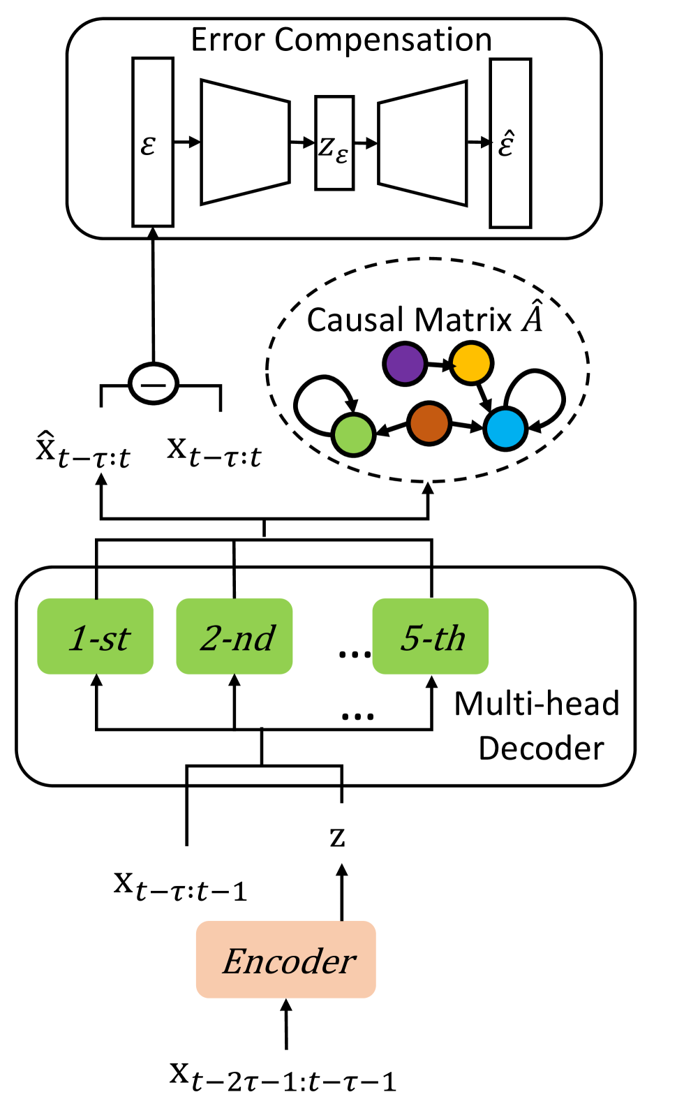
(c) The pipeline of CR-VAE. The multi-head decoder predicts $5$ variables separately in training; The compensation network approximates $\varepsilon_{t}$ in Eq. (3). The adjacency matrix $\hat{A}$ of Granger causal graph $\hat{A}$ can be obtained by stacking, i.e., $\hat{A}=\{\hat{A}_{1};\hat{A}_{2};\hat{A}_{3};\hat{A}_{4};\hat{A}_{5}\}$.

Figure 1: Architecture of Causal Recurrent Variational Autoencoder (CR-VAE). We use a $5$-variate time series as an example.

Both encoder and decoder of our causal recurrent variational autoencoder (CR-VAE) consist of recurrent neural networks such that the hidden state is calculated based on the previous state and the observation at the current time instant. A CR-VAE model with time lag $\tau$ can be written as:

$$\hat{\mathbf{x}}_{t-\tau:t}=D_{\theta}(\mathbf{x}_{t-\tau:t-1},E_{\phi}(\mathbf{x}_{t-2\tau-1:t-\tau-1}))+\varepsilon_{t},$$ (4)

where $D_{\theta},E_{\phi}$ represent decoder and encoder, which are parameterized by $\theta$ and $\phi$, respectively; $\varepsilon_{t}$ is the additive innovation term that has no specific distributional assumption.

Our CR-VAE takes as input the segment $\mathbf{x}_{t-2\tau-1:t-\tau-1}$, and aims to predict or reconstruct the segment $\mathbf{x}_{t-\tau:t}$ step-wisely. In this way, we obey the principle of Granger causality by preventing encoding future information before decoding. By contrast, other popular recurrent VAEs, such as VRAE (Fabius and Van Amersfoort 2014), SRNN (Fraccaro et al. 2016), Z-forcing (Goyal et al. 2017), use the same time segment in both encoder and decoder, thereby encoding future information in the recurrent structure. Our training model is in fact motivated by T-forcing (Williams and Zipser 1989) and other predictive autoregressive models (e.g., (Litterman 1986; Bengio et al. 2015)) that use the real past observations to predict the current value in the sequence.

Another distinction between CR-VAE and other popular recurrent VAEs (Fabius and Van Amersfoort 2014; Chung et al. 2015; Goyal et al. 2017) is that our decoder has multiple heads, in which the $p$-th head is used to approximate $f_{p}\left(\mathbf{x}_{t-}^{p},\text{PA}(\mathbf{x}_{t}^{p})_{t-}\right)$ in Eq. (3). Then, the full vector $\hat{\mathbf{x}_{t}}$ is constructed by stacking the output of all $M$ heads. In short, the term $D_{\theta}(\mathbf{x}_{t-\tau:t-1},E_{\phi}(\mathbf{x}_{t-2\tau-1:t-\tau-1}))$ learns to estimate a collection of $\{f_{p}(\cdot)|p=1,2...M\}$.

Fig. 1(a) shows the structure of our encoder. Let $h$ be hidden states in our encoder, our encoder can be written as:

$$\mathbf{h}_{t}=\text{tanh}(W_{in}\mathbf{x}_{t}+W_{h}\mathbf{h}_{t-1}+b),$$ (5)

$$\mu=W_{\mu}\mathbf{h}_{t-\tau-1}+b_{\mu},$$

$$\log(\sigma)=W_{\sigma}\mathbf{h}_{t-\tau-1}+b_{\sigma},$$

where $\{W_{in},W_{h},W_{\mu},W_{\sigma}\}\subseteq\theta$. $W_{in}$ and $W_{h}$ are the weight matrix for inputs and hidden states, respectively; $W_{\mu}$ and $W_{\sigma}$ are the weights to compute mean and standard deviation of the learned Gaussian distribution, respectively; $b$ denotes the bias.

Fig. 1(b) shows the structure of the $1$-st head of our decoder, in which we use a $5$-variate time series as an example. The collection of all heads explicitly models $p(\mathbf{x}_{t}|\mathbf{x}_{1:t-1})$. Let $\mathbf{s}$ be the hidden state in our decoder. The initial state of decoder is sampled from the Gaussian distribution parameterized by $\mu$ and $\sigma$. More formally, we have:

$$\mathbf{s}_{t-\tau}=\text{tanh}((U_{re}(\mu+\sigma\mathbf{z})+b_{re}),$$ (6)

$$\mathbf{z}\sim N(0,I),$$

$$\mathbf{s}^{p}_{t}=\text{tanh}(U^{p}_{in}\mathbf{x}_{t-1}+U^{p}_{h}\mathbf{s}^{p}_{t-1}+b^{p}),$$

$$\hat{A}_{p}=U^{p}_{in},$$

$$\hat{\mathbf{x}}^{p}_{t}=U^{p}_{out}\mathbf{s}^{p}_{t}+b^{p}_{out},$$

where $\{U^{p}_{in},U_{re},U^{p}_{h},U^{p}_{out}\}\subseteq\phi$. $U^{p}_{in}$ and $U^{p}_{h}$ denote weight matrix for inputs and hidden states of the $p$-th head in the decoder. Similarly, $U_{re}$ and $U^{p}_{out}$ denote weights for reparameterization and output layers; $\hat{A}_{p}$ is the $p$-th row of the estimated adjacency matrix $\hat{A}$ of the Granger causal graph, which includes all cause variables of the $p$-th variable. Note that, we use a single-layer vanilla RNN as an example for simplicity. In practice, we use gated recurrent units (GRUs) (Cho et al. 2014) to improve modeling ability.

Fig. 1(c) shows the pipeline of full model. An error compensation network is applied to model an additive innovation term $\varepsilon_{t}$ in Eq. (4), thus further improving sequence generation performance. We assume $\varepsilon_{t}$ is not predictable or inferable by the information of the past. To compensate for it, another recurrent VAE parameterized by $\{\psi,\omega\}$, is utilized to estimate the additive noise $\varepsilon_{t-\tau:t}$. Here, we use the same sequence as inputs for both encoder and decode, since it does not disentangle the obtained causal graph $\hat{A}$.

CR-VAE Loss Function

In order to estimate $A$ in the process of learning, we invoke a sparsification trick which is first shown in neural Granger causality (NCG) (Tank et al. 2021) and has also been used in recent causal discovery literature (Marcinkevičs and Vogt 2021; Liu et al. 2020). The essential sparsification trick is simple. It assumes that the causal matrix $A$ is sparse and applies sparsity-inducing penalty to $\hat{A}$. It shares the theme with the traditional prediction-based Granger causality – the causes help predict the effects. Therefore, we train CR-VAE by minimizing the following penalized loss function with the stochastic gradient descent (SGD) and proximal gradients:

$$\mathcal{L}(\theta,\phi)=\sum_{p=1}^{M}\left[\mathbb{E}_{q_{\phi}(\mathbf{z}|\mathbf{x}_{t-2\tau-1:t-\tau-1})}[{\rm log}p_{\theta}(\mathbf{x}^{p}_{t-\tau:t}|\mathbf{x}_{t-\tau:t-1},\mathbf{z})]\right]$$ (7)

$$-\mathcal{D}_{KL}(q_{\phi}(\mathbf{z}|\mathbf{x}_{t-2\tau-1:t-\tau-1})||p(\mathbf{z}))+\lambda R(\hat{A}),$$

where $p(\mathbf{z})$ is a standard Normal distribution. The loss function includes three terms: (1) the mean squared error (MSE) loss pushes the model towards high fidelity to sample space; (2) the KL divergence term ensures that the latent space behaves as a Gaussian emission; and (3) a sparsity-inducing penalty term $R(\cdot)$ on $\hat{A}$ with a hyper-parameter $\lambda$. The first two terms correspond to our multi-head recurrent VAE.

Meanwhile, the additional $\varepsilon$ compensation network of CR-VAE is trained by minimizing:

$$\mathcal{L}(\psi,\omega)=\mathbb{E}_{q_{\omega}(\mathbf{z}_{\varepsilon}|\varepsilon_{t-\tau:t})}{\rm log}p_{\psi}(\varepsilon_{t-\tau:t}|\mathbf{z}_{\varepsilon})$$ (8)

$$-\mathcal{D}_{KL}(q_{\omega}(\mathbf{z}_{\varepsilon}|\varepsilon_{t-\tau:t})||p(\mathbf{z}_{\varepsilon})).$$

This is a standard VAE objective function, and its update does not affect the result of $\hat{A}$.

CR-VAE Learning and Optimization

The ideal choice of $R(\cdot)$ is the $\ell_{0}$ norm which represents the number of non-zero elements, but the optimization of $\ell_{0}$ norm in neural network is still challenging. Hence we apply $\ell_{1}$ norm, and the Eq. (7) becomes a typical lasso problem. Proximal gradient descent is the most popular method for non-convex lasso objective optimization. In practice, we use iterative shrinkage-thresholding algorithms (ISTA) (Daubechies, Defrise, and De Mol 2004; Chambolle et al. 1998) with fixed step size. The feature of thresholding leads to exact zero solutions in $U^{p}_{in}$. More formally, we start to update weights $U^{p}_{in}$ iteratively from $U^{p}_{in}(0)$:

$$U^{p}_{in}(i+1)={\rm prox}_{\gamma}(U^{p}_{in}(i)-\gamma\nabla\mathcal{L}_{c}(U^{p}_{in}(i))),$$ (9)

where ${\rm prox}_{\gamma}$ denotes the proximal operator with step size $\gamma$; $\mathcal{L}_{c}$ denotes the convex part of the loss function that is the first and second term in Eq. (7). During training, two separate optimization methods are implemented: proximal gradient on the weights of input layers $U^{p}_{in}$, and stochastic gradient descent (SGD) on all other parameters.

It performs well in causal discovery, but reduces the generation performance since we invoke $\ell_{1}$ norm as our sparsity penalty. To solve this problem, we propose a two-stage training strategy inspired by network pruning (Liang et al. 2021), as summarized in Algorithm 1. In line 1-8, we train the CR-VAE with both proximal gradient and SGD to obtain the sparse causal graph (Phase I); In line 9, we fix the zero elements; In line 10-13, we continue training CR-VAE with SGD to improve generation performance (Phase II).

Once the CR-VAE has been trained, we can obtain the estimated causal matrix by stacking $U^{p}_{in}$, and it can also be used for synthetic sequence generation. During sequence generation, we independently sample two sets of noise $\mathbf{z}$ and $\mathbf{z}_{\varepsilon}$, and then feed them to the decoders to iteratively generate a time series of arbitrary length.

Algorithm 1 Training pipeline of CR-VAE

Require: The multivariate time sequence $\{\mathbf{x}_{t}\}^{T}_{t=1}$ with $M$ dimensions; model lag $\tau$; step size $\gamma$ for ISTA; initialize $\{\theta,\phi,\psi,\omega\}$
Output: Estimated adjacency matrix $\hat{A}$ of Granger causal graph, the trained $\{\theta,\phi,\psi,\omega\}$.

1:  while not stop criteria or converge do

2:     Sample a batch of $\mathbf{x}_{t-2\tau-1:t}$ from $\{\mathbf{x}_{t}\}^{T}_{t=1}$.

3:     Compute the gradients of $\mathcal{L}_{c}$, i.e, convex terms in Eq. (7).

4:     Update $\theta,\phi$ except $U_{in}$ using SGD.

5:     Update $U_{in}$ using proximal gradient descent in Eq. (9).

6:     Update $\psi,\omega$ by minimizing Eq. (8).

7:  end while

8:  Stack $U_{in}$ to obtain the $M\times M$ estimated causal matrix $\hat{A}$.

9:  Prune out all zeros edges in $U_{in}$ based on $\hat{A}$.

10:  while not or converge do

11:     Compute the gradients of $\mathcal{L}_{c}$.

12:     Update $\theta,\phi$ using SGD.

13:     Update $\psi,\omega$ by minimizing Eq.‘(8).

14:  end while

15:  return $\hat{G}$, trained $\{\theta,\phi,\psi,\omega\}$.

Experiments

We first evaluate CR-VAE on a synthetic linear autoregressive process to illustrate the importance of each module. We then compare CR-VAE with several state-of-the-art (SOTA) approaches on four benchmark time series datasets to demonstrate its advantages in both causal discovery and synthetic time series generation.

Linear Autoregressive Process

CR-VAE features a few special designs over the traditional RVAE, such as the multi-head decoder, the unidirectional inputs and the error-compensation module. To illustrate the importance of each component to the performance gain, we first test CR-VAE on a synthetic linear multivariate autoregressive process with $10$ dimensions and maximum lag of $3$. More formally:

$$\mathbf{x}_{t}=a_{1}\mathbf{x}_{t-1}+a_{2}\mathbf{x}_{t-2}+a_{3}\mathbf{x}_{t-3}+\varepsilon_{t},$$ (10)

where $\varepsilon_{t}\sim N(0,I)$; the true causal matrix $G$ can be represented by all non-zeros elements of the $a_{1}+a_{2}+a_{3}$.

Unidirectional Inputs: Don’t Peep on the Future.

The original VRAE and its recent variants (Goyal et al. 2017; Fabius and Van Amersfoort 2014) use $\mathbf{x}_{t-\tau:t-1}$ as the input of both encoder and decoder. This way, information of the entire sequence is encoded before decoding. Those approaches estimate $p(x_{t}|x_{1:T})$, rather than $p(x_{t}|x_{1:t-1})$, i.e., the future input values at time $t$ cannot be used in the conditional variable. This is called causal conditioning as proposed by Massey and Kramer (Kramer 1998). From a causal discovery perspective, it violates the underlying principles of Granger causality by “peeping on the future” and hence can never identify causality in the sense of Granger.

To support our argument, we take $\mathbf{x}_{t-\tau:t-1}$ as the input of encoder (rather than $\mathbf{x}_{t-2\tau-1:t-\tau-1}$). We term this modification the non-unidirectional CR-VAE. As shown in Fig. 2, CR-VAE identifies majority of true causal relations, whereas its non-unidirectional baseline, whose encoder peeps on future values, fails to discover causal directions between most pairs of time series.

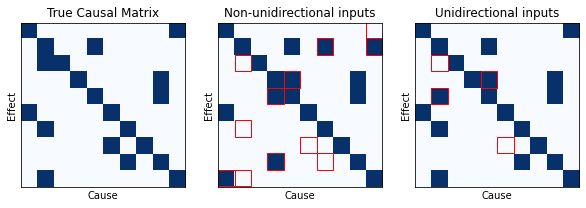
Figure 2: (a) shows the true adjacency matrix $A$ of Granger causal graph; (b) and (c) show the recovered adjacency matrix $\hat{A}$ by non-unidirectional CR-VAE and our CR-VAE. False causal relations are highlighted by red rectangles.

Error-Compensation Network.

We then validate the indispensability of error-compensation network. We compare the time series generation results of the original CR-VAE and its degraded version without error-compensation. We use t-SNE (Van der Maaten and Hinton 2008) to visualize the generated samples. A good generative model should lead to similar synthetic distribution to real data distribution. As shown in Fig. 3, the error-compensation network leads to a significant performance gain. In fact, samples generated by CR-VAE without error-compensation converge quickly to values nearly zero. This makes sense for a linear AR process, because it can only diverge to $\infty$ or converge to nearly zero if we omit $\varepsilon_{t}$ in Eq. 10. In our case, we tune values of $\{a_{1},a_{2},a_{3}\}$ to avoid divergence, and the true $\mathbf{x}_{t}=a_{1}\mathbf{x}_{t-1}+a_{2}\mathbf{x}_{t-2}+a_{3}\mathbf{x}_{t-3}$ did converge. In other words, the degraded CR-VAE captures the dynamics $p(\mathbf{x}_{t}\mid\mathbf{x}_{1:t-1})$, but ignores $\varepsilon_{t}$.

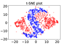
t-SNE without compensation

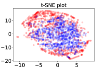
t-SNE with compensation

Figure 3: t-SNE visualization on the illustrative linear system: red samples correspond to real time series, whereas blue samples correspond to synthetic time series.

Experiments on Different Data

We then systematically evaluate the performances of CR-VAE in causal discovery and time series generation on four widely used time series data.

• Hénon maps: We select $6$ coupled Hénon chaotic maps (Kugiumtzis 2013), whose true causal relation is $x^{i-1}\rightarrow x^{i}$. We generate $2,048$ samples to constitute our training data. Equations can be found in supplementary material.

• Lorenz-96 model: It is a nonlinear model formulated by Edward Lorenz in $1996$ to simulate climate dynamics (Lorenz 1996). The $p$-dimensional Lorenz-96 model is defined as:

  $$\frac{d\mathbf{x}_{t}^{i}}{dt}=(\mathbf{x}^{i+1}-\mathbf{x}^{i-2})\mathbf{x}^{i-1}-\mathbf{x}^{i}+F,$$ (11)

  where $\mathbf{x}^{-1}=\mathbf{x}^{p-1}$, $\mathbf{x}^{0}=\mathbf{x}^{p}$ and $\mathbf{x}^{p+1}=\mathbf{x}^{1}$. $F$ is the forcing constant which is set to be $10$. We take $p=10$ and generate $2,048$ samples as training data.

• fMRI: It is a benchmark for causal discovery, which consists of realistic simulations of blood-oxygen-level-dependent (BOLD) time series (Smith et al. 2011) generated using the dynamic causal modelling functional magnetic resonance imaging (fMRI) forward model. Here, we select simulation no. 3 of the original dataset. It has $10$ variables, and we randomly select $2,048$ observations.

• EEG: It is a dataset of real intracranial EEG recordings from a patient with drug-resistant epilepsy (Kramer, Kolaczyk, and Kirsch 2008). We select 12 EEG time series from 76 contacts since they are recorded at deeper brain structures than cortical level. Note, however, that there is no ground truth of causal relation in this dataset.

Causal Discovery Evaluations

We compare CR-VAE with $4$ popular Granger causal discovery approaches. They are: kernel Granger causality (KGC) (Marinazzo, Pellicoro, and Stramaglia 2008) that uses kernel trick to extend linear Granger causality to non-linear scenario; transfer entropy (TE) (Schreiber 2000) estimated by the matrix-based Rényi’s $\alpha$-order entropy functional (Giraldo, Rao, and Principe 2014); Temporal Causal Discovery Framework (TCDF) (Nauta, Bucur, and Seifert 2019) which integrates attention mechanism into a neural network; Neural Granger causality (NGC) (Tank et al. 2021), which is the first neural network-based approach for Granger causal discovery.

KGC and TE rely on information-theoretic measures (on independence or conditional independence) and post-processing (e.g., hypothesis test), whereas TCDF, NGC and our CR-VAE are neural network-based approaches that obtain causal relations actively and automatically in a learning process. All methods are trained only on one sequence that is stochastically sampled based on lag. We use true lag for KGC and TE and set it to be $10$ for TCDF, NGC and CR-VAE. For each approach, we compare the estimated causal adjacency matrices with respect to the ground-truth and apply areas under receiver operating characteristic curves (AUROC) as a quantitative metric. For neural network-based approaches, we select the estimated causal matrices by searching smallest convex loss. Relevant hyper-parameters of all learnable models are tuned to minimize the loss function. Details can be found in supplementary material.

Table 4 summarizes the quantitative comparison results. The neural network-based approaches outperform traditional KGC and TE by a considerable margin. This is because traditional approaches are incapable of detecting self-causes. Our CR-VAE outperforms TCDF in all datasets and achieves similar performance to NGC. This can be expected. Note that, both CR-VAE and NGC apply $\ell_{1}$ sparsity penalty on network weights to discover causal relations.

Although the ground-truth causal relation of EEG data is not available, we compare the estimated causal matrices by our method and KGC in Fig. 4. We observed that most of causal relations in our estimation are concentrated on the last six sequences, whereas the causal elements found by KGC distribute more evenly. Our results make more sense because doctors often perform anterior jaw lobectomy for patients with epilepsy by resecting the last six contact areas (Stramaglia, Cortes, and Marinazzo 2014; Kramer, Kolaczyk, and Kirsch 2008). KGC fails to capture this.

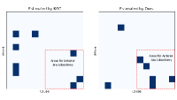
Figure 4: Estimated causal adjacency matrix (without self-causal elements) of KGC and CR-VAE on EEG data. Our causal elements concentrate in the last six sequence.

Methods	KGC	TE	TCDF	NGC	Ours
Hénon	0.465	0.465	0.911	0.960	0.960
Lorenz	0.631	0.408	0.871	0.980	0.954
fMRI	0.379	0.380	0.881	0.950	0.957

Table 1: Comparison of causal discovery using AUROC on Hénon, Lorenz-96 and fMRI. The best performance is in bold. The second-best performance is underlined.

Time Series Generation Evaluation

In time series generation, we compare CR-VAE with $3$ baselines: Time-series generative adversarial network (TimeGAN) (Yoon, Jarrett, and Van der Schaar 2019) that takes transition dynamics into account under the framework of GAN; the popular variational RNN (VRNN) (Chung et al. 2015); and the variational recurrent autoencoder (VRAE) (Kingma and Welling 2013) which is the backbone of our approach.

We first qualitatively evaluate the quality of generated time series by projecting both real and synthetic ones into a $2$-dimensional space with t-SNE. A good generative model is expected to encourage close distributions for real and synthetic data. As can be seen from Fig. 5, CR-VAE demonstrates markedly better overlap with the original data than TimeGAN and performs slightly better than VRAE. On fMRI data, it is almost impossible to distinguish our generated samples with respect to real ones. This result further demonstrate the great potential of our CR-VAE in other medical applications.

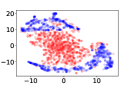
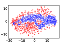
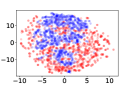
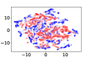
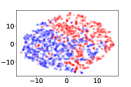
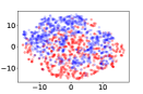
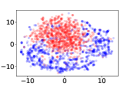
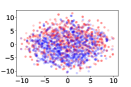
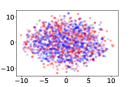
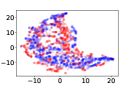
TimeGAN

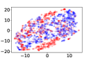
VRAE

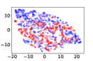
Ours

Figure 5: t-SNE visualization on Henon (1st row), Lorenz 96 (2nd row), fMRI (3rd row) and EEG (4th row). Red samples correspond to real time series, whereas blue samples correspond to synthetic time series.

Next, we adopt the maximum mean discrepancy (MMD) (Gretton et al. 2006) and the “train on synthetic and test on real” (TSTR) strategy to further evaluate the performances of different methods quantitatively. Specifically, MMD is utilized to measure the distance between generated data and real data. Same to (Goudet et al. 2018), we take account of a bandwidth of kernel size $[0.01,0.1,1,10,100]$. For TSTR, we use synthetic samples to train a sequential prediction neural network with LSTM-RNN layers to predict next samples. Then we test the trained model on real time series. Prediction performance is measured by root mean square error (RMSE). Intuitively, if a generative model captures well the underlying dynamics of a real time series (i.e., $p(\mathbf{x}_{t}|\mathbf{x}_{1:t-1})$), it is expected to have low prediction error under TSTR framework.

As shown in Table 5, CR-VAE consistently generates higher-quality synthetic data in comparison to baselines. For fMRI, our result is slightly outperformed by VRAE. This is because CR-VAE fails to discover some causal relations.

Metric	Methods	Henon	Lorenz	fMRI	EEG
	TimeGAN	0.476	0.040	0.157	0.064
MMD	VRNN	0.324	0.043	0.145	0.072
	VRAE	0.125	0.010	0.011	0.107
	Ours	0.118	0.015	0.010	0.050
	TimeGAN	0.297	0.124	0.163	0.042
TSTR	VRNN	0.185	0.131	0.233	0.054
	VRAE	0.125	0.088	0.119	0.030
(RMSE)	Ours	0.122	0.056	0.122	0.024
	Real (TRTR)	0.024	0.017	0.107	0.010

Table 2: Quantitative comparison with MMD and TSTR. The best performance is in bold. The second-best performance is underlined.

Conclusion

We develop a unified model, termed causal recurrent variational autoencoder (CR-VAE), that integrates the concepts of Granger causality into a recurrent VAE framework. CR-VAE is able to discover Granger causality from past observations to present values between pairwise variables and within a single variable. Such functionality makes the generation process of CR-VAE more transparent. We test CR-VAE in two synthetic dynamic systems and two benchmark medical datasets. Our CR-VAE always has smaller maximum mean discrepancy values and prediction mean square errors using the “train on synthetic and test on real” strategy.

Future works are twofold. First, same to other Granger causality approaches, our model assumes no unmeasured confounders. Second, an isotropic Gaussian assumption for latent factors limits our generative capability. We will continue the design of time series generative models to account for latent confounders and more flexible latent distributions.

Supplementary Material

This document contains the supplementary material for the “Causal Recurrent Variational Autoencoder for Medical Time Series Generation” manuscript. It is organized into the following topics and sections:

1. More on Related Works

2. Details of Experimental Setting

   1. More Details of Dataset

   2. Details of Traditional Granger Causality

   3. Details of Neural Network-based Approaches of Granger Causality

   4. Details of Generation

3. Additional Experimental Results

   1. Adjacency Matrices of Granger Causal Summary Graphs

   2. Synthetic Time Series by Different Methods

   3. Prediction Results of TSTR

   4. PCA Visualization

   5. Ablation Study of the Two-Stage Training Strategy

4. Minimal Structure of CR-VAE in PyTorch and Code Link

More on Related Works

Different types of causal graphs can be considered for time series (Assaad, Devijver, and Gaussier 2022b). The window causal graph (see Fig. 6(a)) only covers a fixed number of time instants (with a maximum causal influence lag $\tau$) and assumes the causal relations amongst different variables are consistent over time. The summary causal graph (see Fig. 6(b)) directly relates variables without any indication of time. Usually, it is difficult to estimate window causal graph because it requires to determine which exact time instant is the cause of another. It is of course easier to estimate a summary causal graph (Assaad, Devijver, and Gaussier 2022a). In practice, it is often sufficient to know the causal relations between time series as a whole, without knowing precisely the relations between time instants (Assaad, Devijver, and Gaussier 2022b).

In our work, we consider recovery of a Granger causal graph (see Fig. 6(c)), which separates past observations and present values of each variable and aims to if the past of $\mathbf{x}^{p}$ (denoted $\mathbf{x}_{t-}^{p}$) causes the present value of $\mathbf{x}^{q}$ (denoted $\mathbf{x}_{t}^{q}$). Obviously, our Granger causal graph lies between window causal graph and summary causal graph.

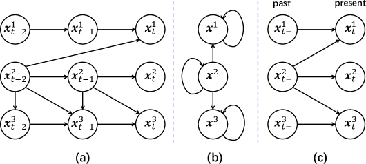
Figure 6: Example of (a) window causal graph; (b) summary causal graph; and (c) our Granger causal graph. Figure adapted from (Assaad, Devijver, and Gaussier 2022a).

Substantial efforts have been made on the causal discovery of time series. The most two popular approaches in this topic are the Granger causality-based approach and the constraint-based approach. The former typically assumes that the past of a cause is necessary and sufficient for optimally forecasting its effect, whereas the latter firstly exploits conditional independencies to build a skeleton between each dimension and then orients the skeleton according to a set of rules that define constraints on admissible orientations (e.g., the PC algorithm with momentary conditional independence (PCMCI) (Runge et al. 2019)). Other well-known approaches include the noise-based approach (e.g., the Time Series Models with Independent Noise (TiMINo) (Peters, Janzing, and Schölkopf 2013)) and the score-based approach (e.g., the DYNOTEARS (Pamfil et al. 2020)). Our model belongs to the Granger causality-based approach.

Details of Experiment Setting

More Details of Dataset

The equations of our Hénon chaotic dataset can be written as:

$$\centering\begin{array}[]{lr}\mathbf{x}^{1}_{t+1}=1.4-(\mathbf{x}^{1}_{t})^{2}+0.3\mathbf{x}^{1}_{t-1},\\ \mathbf{x}^{p}_{t+1}=1.4-(e\mathbf{x}^{p-1}_{t}+(1-e)\mathbf{x}^{p}_{t})^{2}+0.3\mathbf{x}^{p}_{t-1},\end{array}\@add@centering$$ (12)

where $p=2,.....K$. The true direct causal relations are $\mathbf{x}^{p-1}\rightarrow\mathbf{x}^{p}$ and self-causal relations $\mathbf{x}^{p}\rightarrow\mathbf{x}^{p}$, i.e., the index of positive elements should be $(p,p-1)$. The length of lag is $2$ while $e=0.3$, $K=6$.

Table 3 summarizes the crucial statistics of four datasets. We conduct our experiments using more than $2,000$ samples on each dataset. For Henon and Lorenz $96$, we sample initial values from standard Gaussian distribution, and then infer the trajectories using transition functions. The fMRI is different from other datasets since it is not a long sequence but $50$ subjects of time sequences. Therefore, we crop them in shorter clips according to models’ lag and randomly select $2,048$ clips to train models. The true lag is not available on fMRI. The EEG data consists of time sequences from $76$ nodes. The first $64$ nodes record the EEG signals through a $8\times 8$ grid at the cortical level (CE), while the other $12$ are placed at deeper brain structures (DE). Therefore, we select the last $12$ contacts as our dataset. We also reassign the values of each node to $[0,1]$ for normalization. Ground truth of causal relations is not available on EEG data.

Dataset	Number of Samples	Number of Variables	True Lag	Number of Causal Relations
Hénon	2048	6	2	11
Lorenz	2048	10	3	40
fMRI	2048	10	NA	21
EEG	5000	12	NA	NA

Table 3: Statistics of Datasets. NA notes ground truth is not available.

Details of Traditional Granger Causality

For kernel Granger causality (KGC), we use the official MATLAB code from authors . For transfer entropy (TE), we follow (De La Pava Panche, Alvarez-Meza, and Orozco-Gutierrez 2019) and estimate information theoretic metrics using the matrix-based Rényi’s $\alpha$-order entropy functional (Sanchez Giraldo, Rao, and Principe 2015). Suppose there are $N$ samples for the $p$-th variable, i.e., $\mathbf{x}^{p}=[\mathbf{x}^{p}(1),\mathbf{x}^{p}(2),\cdots,\mathbf{x}^{p}(N)]$ where the numbers in parentheses denotes sample index. A Gram matrix $K^{p}\in\mathbb{R}^{N\times N}$ can be obtained by computing $K^{p}(n,m)=\kappa(\mathbf{x}^{p}(n),\mathbf{x}^{p}(m))$, where $\kappa$ is a Gaussian kernel with kernel width $\sigma$. The entropy of $\mathbf{x}^{p}$ can be expressed by (Sanchez Giraldo, Rao, and Principe 2015):

$$H_{\alpha}(\mathbf{x}^{p})=H_{\alpha}(A^{p})=\frac{1}{1-\alpha}\log_{2}[\sum_{n=1}^{N}\lambda_{n}(A^{p})^{\alpha}],$$ (13)

where $A^{p}=K^{p}/trace(K^{p})$ is the normalized Gram matrix and $\lambda_{n}(A_{i})$ denotes $n$-th eigenvalue of $A^{p}$.

Further, the joint entropy for $\{\mathbf{x}^{p}\}_{p=1}^{M}$ is defined as (Yu et al. 2020):

$$H_{\alpha}(\mathbf{x}^{1},\mathbf{x}^{2},\cdots,\mathbf{x}^{M})=H_{\alpha}(\frac{A_{1}\circ A_{2}\cdots\circ A_{M}}{trace(A_{1}\circ A_{2}\cdots\circ A_{M})}).$$ (14)

where $\circ$ denotes element-wise product. Give a variable $\mathbf{y}$, We also have the:

$${\rm TE}_{\alpha}(\mathbf{x}\rightarrow\mathbf{y})=H_{\alpha}(\mathbf{y}|\mathbf{y}-)-H_{\alpha}(\mathbf{y}|\mathbf{x}-,\mathbf{y}-),$$ (15)

$$H_{\alpha}(A|B)=H_{\alpha}(A,B)-H_{\alpha}(B),$$

Therefore, we can estimated TE from data directly using Eqs. (13)-(15).

In our experiments, for traditional Granger causal discovery methods (i.e., KGC and TE), the hyperparameters such as the kernel width $\sigma$ are determined by grid search. Results reported in the main manuscript use hyperparameters that achieved the highest AUROC. Details are summarized in Table 4.

Dataset	Method	Lag	Kernel Size	Dataset	Method	Lag	Kernel Size	Dataset	Method	Lag	Kernel Size
Henon	KGC	2	0.1	Lorenz	KGC	5	0.5	fMRI	KGC	5	0.2
	TE	2	0.1		TE	5	0.1		TE	5	0.5

Table 4: Hyper-parameters of traditional Granger causal discovery methods

Details of Neural Network-based Approaches of Granger Causality

For neural network-based methods, we assume a range of sparsity level and then search a grid of hyperparameters that minimize the convex part of their loss functions. With this testing setup, our goal is to fairly compare the performance of neural network-based techniques that rely on sparisty trick. For example, we assume the sparse level of causal relations on Hénon chaotic data ranges from $20\%$ to $40\%$, and then we tune the $\lambda$ of TCDF, NGC and our CR-VAE to converge to this sparsity level. In the end, we tune other hyper-parameters including early stopping by searching lowest loss without the sparsity penalty, i.e., convex part of loss functions. We fix the lag to be $10$ and batch size to be $256$. Other hyper-parameters are shown in Table 5.

Dataset	Method	Sparsity Level Range	Sparsity Coefficient $\lambda$	Hidden Neurons	Hidden Layers
	TCDF	[20% , 40% ]	1	64	2
Henon	NGC	[20% , 40% ]	0.5	64	2
	Ours	[20% , 40% ]	0.2	64	2
	TCDF	[35% , 50% ]	2.5	64	2
Lorenz	NGC	[35% , 50% ]	10	64	2
	Ours	[35% , 50% ]	8	64	2
	TCDF	[15% , 28% ]	1	128	2
fMRI	NGC	[15% , 28% ]	0.5	64	2
	Ours	[15% , 28% ]	0.75	64	2

Table 5: Hyper-parameters of neural-network-based Granger causal discovery methods

Details of Generation

We have two baselines that represent two major tracks of generative models. TimeGAN is a recently proposed state-of-the-art (SOTA) GAN-based generative model for time series that takes transition dynamics $p(\mathbf{x}_{t}|\mathbf{x}_{1:t-1})$ into account and also outperforms other GAN-based generators, such as (Esteban, Hyland, and Rätsch 2017). We use the official codes in tensorflow, and search a range of hyper-parameters starting from default setting of the codes to minimize the MMD between real and generated data. VRAE is a classic extension of VAE for time series data. We replicate the official codes of theano using PyTorch. For both VRAE and our CR-VAE, we searched across a grid of hyper-parameters to minimize MMD.

Evaluation Metrics of Generation

The first metric we apply is the maximum mean discrepancy (MMD) (Gretton et al. 2012) which has been widely used to measure the distance between two distributions. In other words, it quantifies if two sets of samples - one synthetic, and the other for the real data - are generated from the same distribution. More formally, given $n$ samples of real and synthetic, we have:

$$MMD(\mathbf{x},\hat{\mathbf{x}})=\frac{1}{n^{2}}\kappa(\mathbf{x}(i),\mathbf{x}(j))+\frac{1}{n^{2}}\kappa(\hat{\mathbf{x}}(i),\hat{\mathbf{x}}(j))-\frac{2}{n^{2}}\kappa(\mathbf{x}(i),\hat{\mathbf{x}}(j)),$$ (16)

where $\hat{\mathbf{x}}$ and $\mathbf{x}$ denote synthetic and real data, respectively, indexed by $i,j$; kernel $\kappa$ is taken as the Gaussian kernel. We average the results of a bandwidth of kernel size $[0.01,0.1,1,10,100]$, same to (Goudet et al. 2018). The MMD is more informative than either generator or discriminator loss in GAN - based models (Esteban, Hyland, and Rätsch 2017), so we early stop to obtain lowest MMD for generative models.

The second metric we apply is “train on synthetic and test on real” (TSTR) by prediction. In our TSTR experiment, we adopt a two-layer RNN with GRU gates to predict next values using synthetic data. Each layer has 64 neurons. The order (length) of the RNN is fixed to be 10. We minimize the mean square error (MSE) using Adam, and fix the learning rate to be 1e-4. We train the RNN with a batch size of 128. Besides, we also split 10% synthetic data as our validation set for early stopping via cross-validation. Then we test the trained model on real time series and quantify the prediction performance using RMSE. More formally:

$$RMSE(\mathbf{x},\hat{\mathbf{x}})=\frac{1}{M}\sum^{M}_{p=1}\sqrt{\frac{\sum_{t}(\mathbf{x}_{t}-\hat{\mathbf{x}}_{t})^{2}}{T}},$$ (17)

where $\hat{\mathbf{x}}$ and $\mathbf{x}$ denote predicted and true samples on real datasets; $T$ is the length of the time clips; $M$ is the number of dimensions indexed by $p$.

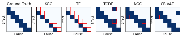
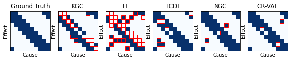
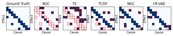
Figure 7: Adjacency matrices on Hénon (1st row), Lorenz 96 (2nd row) and fMRI (3rd row). The $1$-st column provides the visualization for ground truth, while other columns provide matrices estimated by causal discovery techniques. False causal relations are highlighted by red rectangles.

Additional Experimental Results

Adjacency Matrices of Granger Causal Summary Graphs

We provide the ground truth of adjacency matrices of Granger causal graphs and compare them with counterparts estimated by CR-VAE and other competing methods. For traditional Granger causality techniques, we search the thresholds by maximizing AUROC and get rid of all values under the thresholds. For neural-based algorithms, we can directly show the estimated matrices.

False positive or negative elements are highlighted by red squares. As illustrated in Fig. 7, CR-VAE outperforms most of baselines and achieves competitive results among neural network-based methods.

Synthetic Time Series by Different Methods

In this section, we generate synthetic time series of length $20$ using all methods on different datasets. For TimeGAN, we sample a noise from $\mathbf{z}\sim N(0,I)$ and feed it to the generator which outputs sequences of synthetic samples. For VRAE, we sample a noise $\mathbf{z}\sim N(0,I)$ and utilize it as the initial state of decoder RNN. Meanwhile, the first input of decoder RNN is zero. We use the predicted value as the input of the next time step to obtain synthetic sequences step-wisely. Similar to VRAE, our CR-VAE also infers the synthetic sequences step-wisely with an initial state $\mathbf{z}\sim N(0,I)$ and zero input. The difference is that we sample another noise $\mathbf{z}_{\varepsilon}\sim N(0,I)$ for error-compensation network to generate a sequence of innovation terms. They are added step-wisely to the inferred values of decoder RNNs in CR-VAE.

Here, we show $10$ generated sequences for each subplot in Fig. 8 to show the “texture” of time series. We can find that our results are similar to VRAE and outperform TimeGAN.

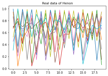
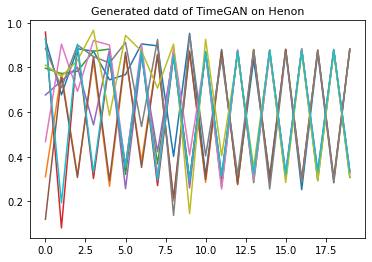
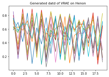
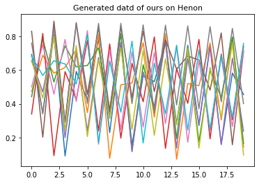
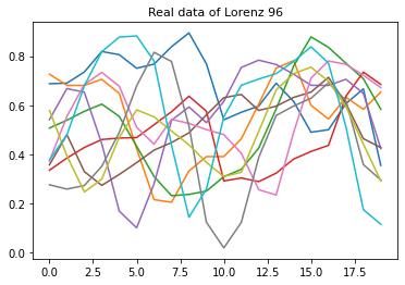
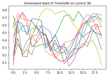
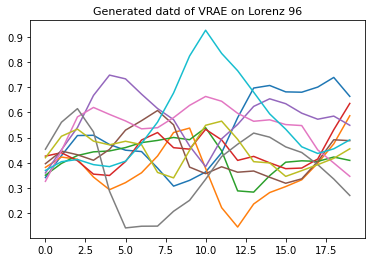
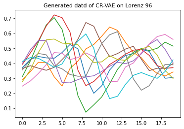
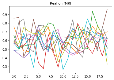
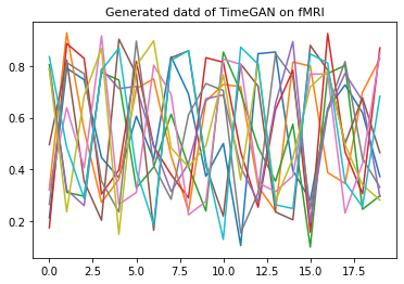
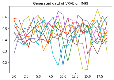
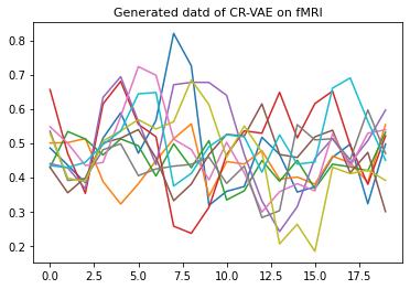
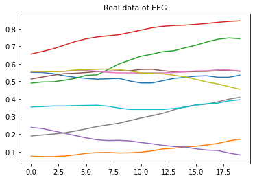
Real Data

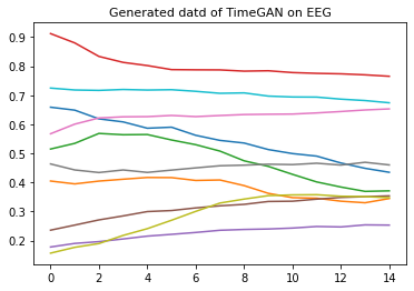
TimeGAN

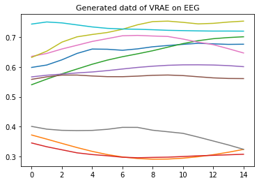
VRAE

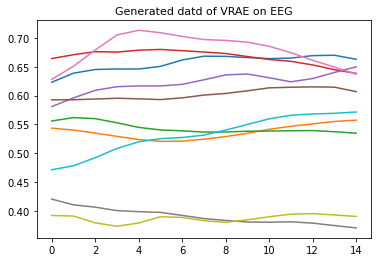
Ours

Figure 8: Generated data on Hénon (1st row), Lorenz 96 (2nd row), fMRI (3rd row) and EEG (4th row). We plot 10 generated sequences to show the texture on average.

 

Prediction Results of TSTR

Up to now, we have quantitatively evaluated our generated samples using TSTR, measured by RMSE. Here, we show the predicted curves to evaluate our generated samples qualitatively. More specific, we train the two-layer RNN on synthetic data generated by CR-VAE, and then use the trained RNN to perform one-step prediction on real data.

Fig. 9 illustrates the $20$-length sequences predicted by CR-VAE, step-wisely on real data. CR-VAE performs quite well on Hénon, Lorenz $96$ and EEG. As can be seen, the predicted curves on Hénon, Lorenz $96$ and EEG demonstrate markedly better overlap with the original curves.

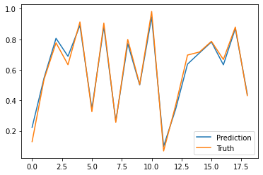
Hénon

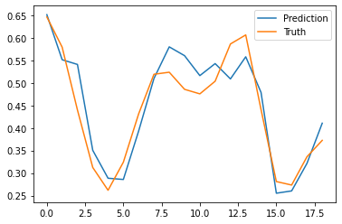
Lorenz 96

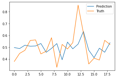
fMRI

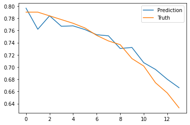
EEG

Figure 9: Prediction Results of CR-VAE on different datasets.

PCA Visualization

Due to page limits, we just show t-SNE visualization in the main manuscript. Here, we qualitatively evaluate the quality of generated time series by projecting both real and synthetic ones into a $2$-dimensional space with PCA in Fig. 10. We expect that a good generative model has close distributions for real and synthetic data, but most of synthetic points overlap with real points well. We conclude that PCA is not a good visualization algorithm for time series since it is not consistent with t-SNE, MMD, and TSTR results that are representative to evaluate generation results. Note, the first PCA plot is quite different from others. This is because synthetic results of TimeGAN on Hénon are clustered to a few fixed values.

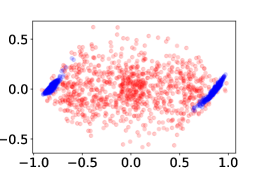
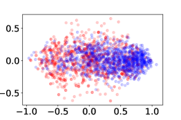
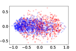
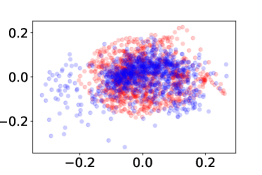
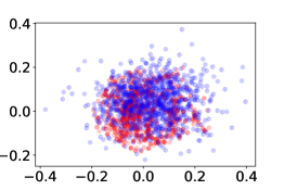
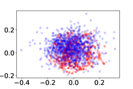
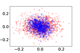
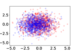
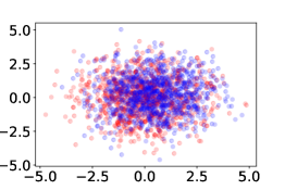
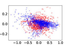
TimeGAN

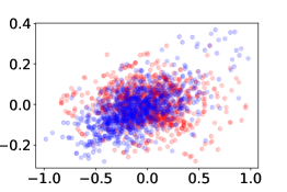
VRAE

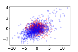
Ours

Figure 10: PCA visualization on Hénon (1st row), Lorenz 96 (2nd row), fMRI (3rd row) and EEG (4th row). Red samples correspond to real time series, whereas blue samples correspond to synthetic time series.

Ablation Study of the Two-Stage Learning Strategy

As we mentioned in the main manuscript, invoking $\ell_{1}$ norm reduces the generation performance since it restricts the solution space of the network. To solve this problem, we propose a two-stage training strategy that we train our model using $\ell_{1}$ norm at first and then stop when the criteria is met or convergence. After that, we fix all zero weights, and continue training other weights using SGD. It improves the performance of generation significantly.

Fig. 11(a) shows the learning curve of CR-VAE on fMRI dataset. We can see that the loss drops significantly after we start our stage II learning. Fig. 11(b) and Fig. 11(c) compare the generation results with and without stage II learning using t-SNE projections. The stage II learning leads to a significant performance gain.

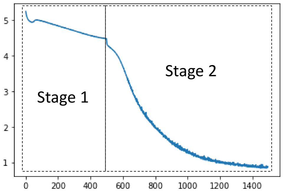
(a) The learning curve on fMRI

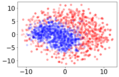
(b) t-SNE without stage 2 learning on fMRI

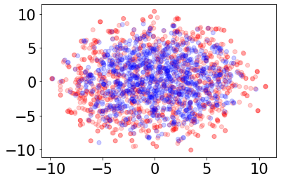
(c) t-SNE with stage 2 learning on fMRI

Figure 11: Learning curve and t-SNE visualization on fMRI: red samples correspond to real time series, whereas blue samples correspond to synthetic time series.

Minimal Structure of CR-VAE in PyTorch and Code Link

PyTorch code of CR-VAE is available at https://github.com/hongmingli1995/CR-VAE.

We also provide the minimal structure of CR-VAE for better understanding.

⬇

1class CRVAE(nn.Module):

2 def __init__(self, num_series, connection, hidden):

3 ”’

4 CRVAE model has num_series decoder GRUs but has only one encoder GRU.

5

6 Args:

7 num_series: Dimension of multivariate time series.

8 connection: Adjacency matrices of causal graphs.

9 Used to prune zero edges in stage 2 learning

10 hidden: Number of units in GRU and 1-D CNN.

11 ’”

12 super(CRVAE, self).__init__()

13

14 self.device = torch.device(’cuda’)

15 self.p = num_series

16 self.hidden = hidden

17

18 self.lstm_left = nn.GRU(num_series, hidden, batch_first=True)

19 self.lstm_left.flatten_parameters()

20

21 self.fc_mu = nn.Linear(hidden, hidden)

22 self.fc_std = nn.Linear(hidden, hidden)

23 self.connection = connection

24

25 # num_series GRUs for num_series time series

26 self.networks = nn.ModuleList([

27 GRU(int(connection[:,i].sum()), hidden) for i in range(num_series)])

28

29 def forward(self, X, hidden=None, mode = ’train’):

30 ”’

31 Args:

32 X: torch tensor of shape (batch_size, Time Length, Dimension).

33 hidden: initail hidden states of GRU.

34 ’”

35 T = X.shape[1]

36 X = torch.cat((torch.zeros(X.shape,device = self.device)[:,0:1,:],X),1)

37

38 ###train the model using real data###

39 if mode == ’train’:

40

41

42 hidden_0 = torch.zeros(1, X.shape[0], self.hidden, device=self.device)

43 out, h_t = self.lstm_left(X[:,1:(T/2)+1,:], hidden_0.detach())

44

45 mu = self.fc_mu(h_t)

46 log_var = self.fc_std(h_t)

47

48 sigma = torch.exp(0.5*log_var)

49 z = torch.randn(size = mu.size())

50 z = z.type_as(mu)

51 z = mu + sigma*z

52

53 pred = [self.networks[i](X, z, self.connection[:,i])[0]

54 for i in range(self.p)]

55

56 return pred, log_var, mu

57

58 ### generate the synthetic date iteratively.###

59 if mode == ’generate’:

60 X_seq = torch.zeros(X[:,:1,:].shape).to(self.device)

61 h_0 = torch.randn(size = (1,

62 X_seq[:,-2:-1,:].size(0),self.hidden)).to(self.device)

63 ht_last =[]

64 for i in range(self.p):

65 ht_last.append(h_0)

66 for i in range(int(T/2)+1):

67

68 ht_new = []

69 for j in range(self.p):

70 out, h_t = self.networks[j](X_seq[:,-1:,:],

71 ht_last[j], self.connection[:,j])

72 if j == 0:

73 X_t = out

74 else:

75 X_t = torch.cat((X_t,out),-1)

76 ht_new.append(h_t)

77 ht_last = ht_new

78 if i ==0:

79 X_seq = X_t

80 else:

81 X_seq = torch.cat([X_seq,X_t],dim = 1)

82

83 return X_seq

References

- Amblard and Michel (2012) Amblard, P.-O.; and Michel, O. J. 2012. The relation between Granger causality and directed information theory: A review. Entropy, 15(1): 113–143.
- Assaad, Devijver, and Gaussier (2022a) Assaad, C. K.; Devijver, E.; and Gaussier, E. 2022a. Causal Discovery of Extended Summary Graphs in Time Series. In The 38th Conference on Uncertainty in Artificial Intelligence.
- Assaad, Devijver, and Gaussier (2022b) Assaad, C. K.; Devijver, E.; and Gaussier, E. 2022b. Survey and Evaluation of Causal Discovery Methods for Time Series. Journal of Artificial Intelligence Research, 73: 767–819.
- Barnett, Barrett, and Seth (2009) Barnett, L.; Barrett, A. B.; and Seth, A. K. 2009. Granger causality and transfer entropy are equivalent for Gaussian variables. Physical review letters, 103(23): 238701.
- Bengio et al. (2015) Bengio, S.; Vinyals, O.; Jaitly, N.; and Shazeer, N. 2015. Scheduled sampling for sequence prediction with recurrent neural networks. Advances in neural information processing systems, 28.
- Chambolle et al. (1998) Chambolle, A.; De Vore, R. A.; Lee, N.-Y.; and Lucier, B. J. 1998. Nonlinear wavelet image processing: variational problems, compression, and noise removal through wavelet shrinkage. IEEE Transactions on Image Processing, 7(3): 319–335.
- Chen, Feng, and Lu (2021) Chen, J.; Feng, J.; and Lu, W. 2021. A Wiener causality defined by divergence. Neural Processing Letters, 53(3): 1773–1794.
- Chen et al. (2004) Chen, Y.; Rangarajan, G.; Feng, J.; and Ding, M. 2004. Analyzing multiple nonlinear time series with extended Granger causality. Physics letters A, 324(1): 26–35.
- Cho et al. (2014) Cho, K.; van Merriënboer, B.; Bahdanau, D.; and Bengio, Y. 2014. On the properties of neural machine translation: Encoder–decoder approaches. In 8th Workshop on Syntax, Semantics and Structure in Statistical Translation, SSST 2014, 103–111. Association for Computational Linguistics (ACL).
- Chu, Glymour, and Ridgeway (2008) Chu, T.; Glymour, C.; and Ridgeway, G. 2008. Search for Additive Nonlinear Time Series Causal Models. Journal of Machine Learning Research, 9(5).
- Chung et al. (2015) Chung, J.; Kastner, K.; Dinh, L.; Goel, K.; Courville, A. C.; and Bengio, Y. 2015. A Recurrent Latent Variable Model for Sequential Data. In Cortes, C.; Lawrence, N.; Lee, D.; Sugiyama, M.; and Garnett, R., eds., Advances in Neural Information Processing Systems, volume 28. Curran Associates, Inc.
- Daubechies, Defrise, and De Mol (2004) Daubechies, I.; Defrise, M.; and De Mol, C. 2004. An iterative thresholding algorithm for linear inverse problems with a sparsity constraint. Communications on Pure and Applied Mathematics: A Journal Issued by the Courant Institute of Mathematical Sciences, 57(11): 1413–1457.
- De La Pava Panche, Alvarez-Meza, and Orozco-Gutierrez (2019) De La Pava Panche, I.; Alvarez-Meza, A. M.; and Orozco-Gutierrez, A. 2019. A data-driven measure of effective connectivity based on Renyi’s -entropy. Frontiers in neuroscience, 13: 1277.
- Desai et al. (2021) Desai, A.; Freeman, C.; Wang, Z.; and Beaver, I. 2021. TimeVAE: A Variational Auto-Encoder for Multivariate Time Series Generation. arXiv preprint arXiv:2111.08095.
- Deshpande et al. (2009) Deshpande, G.; LaConte, S.; James, G. A.; Peltier, S.; and Hu, X. 2009. Multivariate Granger causality analysis of fMRI data. Human brain mapping, 30(4): 1361–1373.
- Esteban, Hyland, and Rätsch (2017) Esteban, C.; Hyland, S. L.; and Rätsch, G. 2017. Real-valued (medical) time series generation with recurrent conditional gans. arXiv preprint arXiv:1706.02633.
- Fabius and Van Amersfoort (2014) Fabius, O.; and Van Amersfoort, J. R. 2014. Variational recurrent auto-encoders. arXiv preprint arXiv:1412.6581.
- Fraccaro et al. (2016) Fraccaro, M.; Sønderby, S. K.; Paquet, U.; and Winther, O. 2016. Sequential neural models with stochastic layers. Advances in neural information processing systems, 29.
- Giraldo, Rao, and Principe (2014) Giraldo, L. G. S.; Rao, M.; and Principe, J. C. 2014. Measures of entropy from data using infinitely divisible kernels. IEEE Transactions on Information Theory, 61(1): 535–548.
- Goodfellow et al. (2014) Goodfellow, I.; Pouget-Abadie, J.; Mirza, M.; Xu, B.; Warde-Farley, D.; Ozair, S.; Courville, A.; and Bengio, Y. 2014. Generative adversarial nets. Advances in neural information processing systems, 27.
- Goudet et al. (2018) Goudet, O.; Kalainathan, D.; Caillou, P.; Guyon, I.; Lopez-Paz, D.; and Sebag, M. 2018. Learning functional causal models with generative neural networks. In Explainable and interpretable models in computer vision and machine learning, 39–80. Springer.
- Goyal et al. (2017) Goyal, A.; Sordoni, A.; Côté, M.-A.; Ke, N. R.; and Bengio, Y. 2017. Z-forcing: Training stochastic recurrent networks. Advances in neural information processing systems, 30.
- Granger (1969) Granger, C. W. J. 1969. Investigating Causal Relations by Econometric Models and Cross-spectral Methods. Econometrica, 37(3): 424.
- Gretton et al. (2006) Gretton, A.; Borgwardt, K.; Rasch, M.; Schölkopf, B.; and Smola, A. 2006. A kernel method for the two-sample-problem. Advances in neural information processing systems, 19.
- Gretton et al. (2012) Gretton, A.; Borgwardt, K. M.; Rasch, M. J.; Schölkopf, B.; and Smola, A. 2012. A kernel two-sample test. The Journal of Machine Learning Research, 13(1): 723–773.
- Hoyer et al. (2008) Hoyer, P.; Janzing, D.; Mooij, J. M.; Peters, J.; and Schölkopf, B. 2008. Nonlinear causal discovery with additive noise models. Advances in neural information processing systems, 21.
- Huijse et al. (2012) Huijse, P.; Estevez, P. A.; Protopapas, P.; Zegers, P.; and Principe, J. C. 2012. An information theoretic algorithm for finding periodicities in stellar light curves. IEEE Transactions on Signal Processing, 60(10): 5135–5145.
- Isaksson, Wennberg, and Zetterberg (1981) Isaksson, A.; Wennberg, A.; and Zetterberg, L. H. 1981. Computer analysis of EEG signals with parametric models. Proceedings of the IEEE, 69(4): 451–461.
- Kingma and Welling (2013) Kingma, D. P.; and Welling, M. 2013. Auto-encoding variational bayes. arXiv preprint arXiv:1312.6114.
- Kramer (1998) Kramer, G. 1998. Causal conditioning, directed information and the multiple-access channel with feedback. In Proceedings. 1998 IEEE International Symposium on Information Theory (Cat. No. 98CH36252), 189. IEEE.
- Kramer, Kolaczyk, and Kirsch (2008) Kramer, M. A.; Kolaczyk, E. D.; and Kirsch, H. E. 2008. Emergent network topology at seizure onset in humans. Epilepsy research, 79(2-3): 173–186.
- Kugiumtzis (2013) Kugiumtzis, D. 2013. Direct-coupling information measure from nonuniform embedding. Physical Review E, 87(6): 062918.
- Liang et al. (2021) Liang, T.; Glossner, J.; Wang, L.; Shi, S.; and Zhang, X. 2021. Pruning and quantization for deep neural network acceleration: A survey. Neurocomputing, 461: 370–403.
- Litterman (1986) Litterman, R. B. 1986. Forecasting with Bayesian vector autoregressions—five years of experience. Journal of Business & Economic Statistics, 4(1): 25–38.
- Liu et al. (2020) Liu, J.; Ji, J.; Xun, G.; Yao, L.; Huai, M.; and Zhang, A. 2020. EC-GAN: inferring brain effective connectivity via generative adversarial networks. In Proceedings of the AAAI Conference on Artificial Intelligence, volume 34, 4852–4859.
- Liu, Pokharel, and Principe (2008) Liu, W.; Pokharel, P. P.; and Principe, J. C. 2008. The kernel least-mean-square algorithm. IEEE Transactions on Signal Processing, 56(2): 543–554.
- Lorenz (1996) Lorenz, E. N. 1996. Predictability: A problem partly solved. In Proc. Seminar on predictability, volume 1.
- Marcinkevičs and Vogt (2021) Marcinkevičs, R.; and Vogt, J. E. 2021. Interpretable models for granger causality using self-explaining neural networks. arXiv preprint arXiv:2101.07600.
- Marinazzo, Pellicoro, and Stramaglia (2008) Marinazzo, D.; Pellicoro, M.; and Stramaglia, S. 2008. Kernel method for nonlinear Granger causality. Physical review letters, 100(14): 144103.
- Massey (1990) Massey, J. 1990. Causality, feedback and directed information. In Proc. Int. Symp. Inf. Theory Applic.(ISITA-90), 303–305.
- Mogren (2016) Mogren, O. 2016. C-RNN-GAN: Continuous recurrent neural networks with adversarial training. Advances in Neural Information Processing Systems (NeurIPS).
- Nauta, Bucur, and Seifert (2019) Nauta, M.; Bucur, D.; and Seifert, C. 2019. Causal discovery with attention-based convolutional neural networks. Machine Learning and Knowledge Extraction, 1(1): 19.
- Pamfil et al. (2020) Pamfil, R.; Sriwattanaworachai, N.; Desai, S.; Pilgerstorfer, P.; Georgatzis, K.; Beaumont, P.; and Aragam, B. 2020. Dynotears: Structure learning from time-series data. In International Conference on Artificial Intelligence and Statistics, 1595–1605.
- Peters, Janzing, and Schölkopf (2013) Peters, J.; Janzing, D.; and Schölkopf, B. 2013. Causal inference on time series using restricted structural equation models. In Advances in Neural Information Processing Systems, volume 26.
- Rangapuram et al. (2018) Rangapuram, S. S.; Seeger, M. W.; Gasthaus, J.; Stella, L.; Wang, Y.; and Januschowski, T. 2018. Deep state space models for time series forecasting. Advances in neural information processing systems, 31.
- Runge et al. (2019) Runge, J.; Nowack, P.; Kretschmer, M.; Flaxman, S.; and Sejdinovic, D. 2019. Detecting and quantifying causal associations in large nonlinear time series datasets. Science advances, 5(11): eaau4996.
- Sanchez Giraldo, Rao, and Principe (2015) Sanchez Giraldo, L. G.; Rao, M.; and Principe, J. C. 2015. Measures of entropy from data using infinitely divisible Kernels. IEEE Trans. Inf. Theory, 61(1): 535–548.
- Schreiber (2000) Schreiber, T. 2000. Measuring information transfer. Physical review letters, 85(2): 461.
- Smith et al. (2011) Smith, S. M.; Miller, K. L.; Salimi-Khorshidi, G.; Webster, M.; Beckmann, C. F.; Nichols, T. E.; Ramsey, J. D.; and Woolrich, M. W. 2011. Network modelling methods for FMRI. Neuroimage, 54(2): 875–891.
- Stramaglia, Cortes, and Marinazzo (2014) Stramaglia, S.; Cortes, J. M.; and Marinazzo, D. 2014. Synergy and redundancy in the Granger causal analysis of dynamical networks. New Journal of Physics, 16(10): 105003.
- Takahashi, Chen, and Tanaka-Ishii (2019) Takahashi, S.; Chen, Y.; and Tanaka-Ishii, K. 2019. Modeling financial time-series with generative adversarial networks. Physica A: Statistical Mechanics and its Applications, 527: 121261.
- Tank et al. (2021) Tank, A.; Covert, I.; Foti, N.; Shojaie, A.; and Fox, E. B. 2021. Neural granger causality. IEEE Transactions on Pattern Analysis and Machine Intelligence.
- Van der Maaten and Hinton (2008) Van der Maaten, L.; and Hinton, G. 2008. Visualizing data using t-SNE. Journal of machine learning research, 9(11).
- Wang et al. (2020) Wang, X.; Wang, R.; Li, F.; Lin, Q.; Zhao, X.; and Hu, Z. 2020. Large-scale granger causal brain network based on resting-state fMRI data. Neuroscience, 425: 169–180.
- West and Harrison (2006) West, M.; and Harrison, J. 2006. Bayesian forecasting and dynamic models. Springer Science & Business Media.
- Wiener (1956) Wiener, N. 1956. The Theory of Prediction. Modern Mathematics for Engineers, 58: 323–329.
- Williams and Zipser (1989) Williams, R. J.; and Zipser, D. 1989. A learning algorithm for continually running fully recurrent neural networks. Neural computation, 1(2): 270–280.
- Yoon, Jarrett, and Van der Schaar (2019) Yoon, J.; Jarrett, D.; and Van der Schaar, M. 2019. Time-series generative adversarial networks. Advances in neural information processing systems, 32.
- Yu et al. (2020) Yu, S.; Giraldo, L. G. S.; Jenssen, R.; and Principe, J. C. 2020. Multivariate extension of matrix-based rényi’s -order entropy functional. IEEE PAMI, 42(11): 2960–2966.