Finite Dimensional Koopman Form of Polynomial Nonlinear Systems

Abstract

The Koopman framework is a popular approach to transform a finite dimensional nonlinear system into an infinite dimensional, but linear model through a lifting process, using so-called observable functions. While there is an extensive theory on infinite dimensional representations in the operator sense, there are few constructive results on how to select the observables to realize them. When it comes to the possibility of finite Koopman representations, which are highly important form a practical point of view, there is no constructive theory. Hence, in practice, often a data-based method and ad-hoc choice of the observable functions is used. When truncating to a finite number of basis, there is also no clear indication of the introduced approximation error. In this paper, we propose a systematic method to compute the finite dimensional Koopman embedding of a specific class of polynomial nonlinear systems in continuous-time such that, the embedding, without approximation, can fully represent the dynamics of the nonlinear system.

1 Introduction

In most engineering fields, due to increasing performance demands, tackling the nonlinear behaviour becomes more and more important. However, the available methods in the field of nonlinear control (e.g. feedback linearization, backstepping, sliding mode control (Khalil, 2002)) are generally complex to design, only offer stability guarantees, and performance shaping of the closed-loop has yet to be achieved. This is in contrast to the systematic and powerful tools available for linear time invariant (LTI) systems. However, using LTI control tools on linearized models offers limited performance when the system evolves away from the operating region. Hence, there is an increasing need to extend the powerful LTI control design and modelling framework to address nonlinear systems. As such, there is a significant interest in finding globally linear surrogate models of nonlinear systems.

One of the more promising approaches to achieve this is given by the Koopman framework (Brunton et al., 2022), (Bevanda et al., 2021), (Mauroy et al., 2020), where the concept is to project the original nonlinear state space representation to a higher dimensional (possibly infinite) but linear space, through observable functions. The Koopman operator is a linear operator and governs the dynamics of the observables. The Koopman framework shows promising results in its application to real-world analysis and control applications (e.g. mechatronic systems (Abraham and Murphey, 2019), (Cisneros et al., 2020), distributed parameter systems (Klus et al., 2020)). For practical use, a finite number of observables needs to be selected. These are then used to construct time shifted data matrices, to compute via least-squares the matrix representation of the Koopman operator. This technique is known as extended dynamic mode decomposition (EDMD) (Williams et al., 2015). However, the main problem is that the choice of the observables is heuristic and there are no guarantees on the quality of the resulting model. To tackle this, one solution is to use data-driven techniques to learn the lifting from data, in order to circumvent the manual selection of observables (Lusch et al., 2018), (Iacob et al., 2021). Nevertheless, this is still an approximation and the questions on how to embed the nonlinear system into an exact linear finite dimensional lifted representation and when this is possible at all are still open. This is an important aspect, because, for control purposes, having an exact finite dimensional embedding allows for the application of the available control tools for linear systems. Moreover, if there exist approximation errors in the model that cannot be quantified, the expected performance will not be achieved. To tackle this, there have been attempts to connect the Koopman framework to immersion (Wang and Jungers, 2020) and Carleman linearization, in order to obtain a clear way of computing the observables. However, in the immersion approach, the existence of a finite dimensional fully linear lifting depends heavily on the observability property of the system and, in general, the resulted embedding contains a nonlinear output injection (Krener and Isidori, 1983), (Jouan, 2003). For the Carleman linearization (Kowalski and Steeb, 1991), while it offers a systematic way of computing the lifting functions, the resulting embedding is still an infinite dimensional model that needs to be trimmed.

The present paper discusses a novel method to systematically convert a polynomial nonlinear system to an exact finite dimensional linear embedding. Starting from the idea of the simple 2-dimensional example shown in (Brunton et al., 2022), we introduce a state-space model where the state equation is described by a lower triangular polynomial form. We prove that there always exists an exact finite dimensional Koopman representation and we show how to systematically compute it. Furthermore, we also show that, once the autonomous part of the nonlinear system is fully embedded, the extension to systems with inputs is trivial and can be performed in a separate step. Using an example system, we demonstrate that the lifted Koopman model can fully capture the original dynamics, both in an autonomous operation and in the presence of inputs.

The paper is structured as follows. Section 2 describes the Koopman framework and details the proof and steps needed to obtain the finite embedding. In Section 3, we discuss the example and showcase the simulation results. In Section 4, conclusions on the presented results are given together with outlooks on future research.

2 Finite dimensional embedding

The present section details the Koopman framework and showcases the proposed method to compute an exact finite dimensional embedding. Additionally, we discuss the extension to systems with inputs.

2.1 Koopman framework

Consider the autonomous nonlinear system:

$$\dot{x}=f(x),$$ (1)

with $x\mathrel{\mathop{\mathchar 58\relax}}=x(t)$ denoting the state, $t\in\mathbb{R}$ represents the time and $f\mathrel{\mathop{\mathchar 58\relax}}\mathbb{R}^{n_{\mathrm{x}}}\rightarrow\mathbb{R}^{n_{\mathrm{x}}}$ is the nonlinear vector field which we consider to be a Lipshitz continuous function. Given an initial condition $x(0)\in\mathbb{X}\subseteq\mathbb{R}^{n_{\mathrm{x}}}$, the solution $x(t)$ can be described as:

$$x(t)=F(t,x(0))\mathrel{\mathop{\mathchar 58\relax}}=x(0)+\int^{t}_{0}f(x(\tau))\operatorname{d\!}\tau.$$ (2)

It is assumed that $\mathbb{X}$ is compact and forward invariant under the flow $F(t,\cdot)$, such that $F(t,\mathbb{X})\subseteq\mathbb{X},\forall t\geq 0$. Introduce the family of Koopman operators $\{\mathcal{K}^{t}\}_{t\geq 0}$ associated to the flow $F(t,\cdot)$ as:

$$\mathcal{K}^{t}\phi(x(0))=\phi\circ F(t,x(0)),\quad\phi\in\mathcal{F},$$ (3)

where, $\mathcal{F}\subseteq\mathcal{C}^{1}$ is a Banach function space of continuously diferetiable functions and $\phi\mathrel{\mathop{\mathchar 58\relax}}\mathbb{X}\rightarrow\mathbb{R}$ is a scalar observable function. As the flow $F$ is uniformly Lipshitz and $\mathbb{X}$ a compact forward-invariant set, the Koopman semigroup $\{\mathcal{K}^{t}\}_{t\geq 0}$ is strongly continuous on $\mathcal{F}$ (Mauroy et al., 2020). Thus, we can describe the infinitesimal generator $\mathcal{L}\mathrel{\mathop{\mathchar 58\relax}}\mathcal{D}_{\mathcal{L}}\rightarrow\mathcal{F}$ associated to the Koopman semigroup of operators (Lasota and Mackey, 1994), (Mauroy et al., 2020) as:

$$\mathcal{L}\phi(x_{0})=\lim_{t\downarrow 0}\frac{\mathcal{K}^{t}\phi(x(0))-\phi(x(0))}{t},\quad\phi\in\mathcal{D}_{\mathcal{L}},$$ (4)

where $\mathcal{D}_{\mathcal{L}}$ is a dense set in $\mathcal{F}$. Note that, as described in (Lasota and Mackey, 1994), the generator $\mathcal{L}$ is a linear operator. Through the infinitesimal generator we can thus describe the dynamics of observables as follows:

$$\dot{\phi}=\frac{\partial\phi}{\partial x}f=\mathcal{L}\phi,$$ (5)

which is a linear infinite dimensional representation of the nonlinear system (1). If there exists a finite dimensional Koopman subspace $\mathcal{F}_{n_{\mathrm{f}}}\subseteq\mathcal{D}_{\mathcal{L}}$, such that the image of $\mathcal{L}$ is in $\mathcal{F}_{n_{\mathrm{f}}}$, then, given the set of lifting functions as basis of $\mathcal{F}_{n_{\mathrm{f}}}$, $\forall\phi\in\Phi$, $\mathcal{L}\phi\in\text{span}\{\Phi\}$. Thus, the following relation holds:

$$\dot{\phi}_{j}=\mathcal{L}\phi_{j}=\sum^{n_{\mathrm{f}}}_{i=1}L_{ij}\phi_{i},$$ (6)

where $L$ denotes the matrix representation of $\mathcal{L}$ and the coordinates of $\mathcal{L}\phi_{j}$ in the basis $\Phi$ are contained in the column $L_{\cdot j}$ Let $A=L^{\top}\in\mathbb{R}^{n_{\mathrm{f}}\times n_{\mathrm{f}}}$, and, based on (5), the lifted representation of (1) is given by:

$$\dot{\Phi}(x)=\frac{\partial\Phi}{\partial x}(x)f(x)=A\Phi(x).$$ (7)

Thus, one can formulate conditions for the existence of a finite dimensional embedding of (1) as:

$$\dot{\Phi} \in\text{span}\{\Phi\},$$ (8a)

which is equivalent to

$$\frac{\partial\Phi}{\partial x}f \in\text{span}\{\Phi\}.$$ (8b)

However, the major question is how to compute $\Phi$ such that the conditions (8) are true. In the Koopman framework, to recover the original states of (1), the existence of a back transformation $\Phi^{\dagger}(\Phi(x))=x$ is often assumed. For simplicity, this is achieved by adding an extra condition to (8), namely that the original states are contained in $\Phi$, i.e., the identity function is part of $\Phi$. Next, in order to explicitly write the LTI dynamics given by the Koopman form, let $z(t)=\Phi(x(t))$. Then, an associated Koopman representation of (1) is:

$$\dot{z}=Az,\quad\text{with }z(0)=\Phi(x(0)).$$ (9)

It is important to note that, by the existing theory, in general one cannot guarantee the existence of a finite dimensional Koopman invariant subspace $\mathcal{F}_{n_{\mathrm{f}}}$. In the sequel we show that, in case of systems described by a state-space representation where the state equation can be written in a lower triangular polynomial form, there always exists an exact finite dimensional Koopman representation of the system in the form of (9) and this representation can be systematically computed.

2.2 Exact finite embedding procedure

Consider the nonlinear system (1) to have the following structure:

$$\begin{split}\dot{x}_{1}&=a_{1}x_{1}\\ \dot{x}_{2}&=a_{2}x_{2}+f_{2}(x_{1})\\ \dot{x}_{3}&=a_{3}x_{3}+f_{3}(x_{1},x_{2})\\ &\vdots\\ \dot{x}_{n}&=a_{n}x_{n}+f_{n}(x_{1},\dots,x_{n-1})\end{split}$$ (10)

where $f_{n}$ is given by:

$$f_{n}(x_{1},\dots,x_{n-1})=\sum^{d_{n}}_{j_{1}=0}\dots\sum^{d_{n}}_{j_{n-1}=0}\alpha^{n}_{j_{1}\dots j_{n-1}}\prod^{n-1}_{i=1}x^{j_{i}}_{i},$$ (11)

with polynomial terms of the form $x^{j_{1}}_{1}\dots x^{j_{n-1}}_{n-1}$. It is assumed that the powers go up to $d_{n}$, for ease of derivation, but there is no restriction and each power can be arbitrarily large (but finite). It could be viewed that $d_{n}$ is the maximum power within the polynomial terms. Under these considerations, we can give the following theorem.

Theorem 1

For an autonomous continuous-time nonlinear system that has a polynomial state-space representation in the form of (10), there exists an exact finite-dimensional lifting $\Phi\mathrel{\mathop{\mathchar 58\relax}}\mathbb{R}^{n_{\mathrm{x}}}\rightarrow\mathbb{R}^{n_{\mathrm{f}}}$, containing the states $x_{i}$, with $i\in\left\{1,\dots,n\right\}$, such that (8a) holds true.

The theorem is proven by induction. First, we will consider the cases when $n=1,2,3,4$ and then we will show that if the statement of Theorem 1 holds for $n$-number of states then we can prove that it also holds for $n+1$.

• $n=1$ (first order system):

  $$\dot{x}_{1}=a_{1}x_{1}$$ (12)

  Let $W_{1}=\{x_{1}\}$ and $\Phi=\mathrm{vec}(W_{1})$, i.e., $\Phi(x)=x_{1}$. It is trivial to see that condition (8a) holds true as $\dot{x}_{1}=a_{1}x_{1}\in\text{span}\{\Phi\}$.

• $n=2$ (second order system): Notice that the dynamics defined by the $2^{\mathrm{nd}}$-order system are described by (12), together with

  $$\dot{x}_{2}=a_{2}x_{2}+\sum^{d_{2}}_{j_{1}=0}\alpha^{2}_{j_{1}}x^{j_{1}}_{1}.$$ (13)

  Here, superscript $2$ of the coefficient $\alpha^{2}_{j_{1}}$ denotes that it belongs to the $2^{\mathrm{nd}}$ state equation and not that the coefficient is raised to power 2. Let $V_{2}=\{x^{0}_{1},\ldots,x^{d_{2}}_{1}\}$ and $W_{2}=\{x_{2}\}\cup V_{2}$, while $\Phi=\mathrm{vec}(W_{1}\cup W_{2})$. By calculating $\dot{\Phi}$, we get the terms associated with $W_{1}$ and the terms

  $$\frac{\operatorname{d\!}}{\operatorname{d\!}t}\left(x^{j_{1}}_{1}\right)=j_{1}x^{j_{1}-1}_{1}\dot{x}_{1}=j_{1}a_{1}x^{j_{1}}_{1}$$ (14)

  originating from $V_{2}$. It is easy to observe that all terms in (14) are already contained in $\Phi$ and $\dot{x}_{2}\in\mathrm{span}\{\Phi\}$, hence condition (8a) holds true.

• $n=3$ (third order system): The dynamics of the $3^{\mathrm{rd}}$-order system are described by (12), (13) and the following equation:

  $$\dot{x}_{3}=a_{3}x_{3}+\sum^{d_{3}}_{j_{1}=0}\sum^{d_{3}}_{j_{2}=0}\alpha^{3}_{j_{1},j_{2}}x^{j_{1}}_{1}x^{j_{2}}_{2}.$$ (15)

  As performed previously, we take the nonlinear terms $x^{j_{1}}_{1}x^{j_{2}}_{2}$ and add them to the set of lifting functions $V_{3}=\{x^{0}_{1}x^{0}_{2},\ldots,x^{d_{3}}_{1}x^{d_{3}}_{2}\}$ and $W_{3}=\{x_{3}\}\cup V_{3}$, while $\Phi=\mathrm{vec}(W_{1}\cup W_{2}\cup W_{3})$. By calculating $\dot{\Phi}$, we get the terms associated with $W_{1}$, $W_{2}$ as before and

  $$\frac{\operatorname{d\!}}{\operatorname{d\!}t} \left(x^{j_{1}}_{1}x^{j_{2}}_{2}\right)=j_{1}x^{j_{1}-1}_{1}x^{j_{2}}_{2}\dot{x}_{1}+j_{2}x^{j_{1}}_{1}x^{j_{2}-1}_{2}\dot{x}_{2}$$ (16)

  $$=(j_{1}a_{1}+j_{2}a_{2})\underbrace{x^{j_{1}}_{1}x^{j_{2}}_{2}}_{a}+j_{2}\sum^{d_{2}}_{\tilde{j}_{1}=0}\alpha^{2}_{\tilde{j}_{1}}\underbrace{x^{j_{1}+\tilde{j}_{1}}_{1}x^{j_{2}-1}_{2}}_{b}$$

  originating from $V_{3}$. The following observations can be made:

  • The terms $a$ are already contained in $V_{3}$.

  • For the terms $b$, we can observe that the power $j_{2}$ decreases by 1 and $j_{1}$ increases by at most $d_{2}$.

  Introduce the operator $\mathfrak{D}_{\mathrm{b}}$ such that $\mathfrak{D}_{\mathrm{b}}(x^{j_{1}}_{1}x^{j_{2}}_{2})=\{x^{j_{1}+\tilde{j}_{1}}_{1}x^{j_{2}-1}_{2}\}_{\tilde{j}_{1}=0}^{d_{2}}$, i.e., it gives the $b$ terms of (16). Then let $V_{3}\leftarrow V_{3}\cup\mathfrak{D}_{\mathrm{b}}(V_{3})$. Repeating the process, i.e., applying the time derivative again to $x^{j_{1}+\tilde{j}_{1}}_{1}x^{j_{2}-1}_{2}$ further decreases $j_{2}$ and increases the power of $x_{1}$, and at each step only terms of the form $a$ and $b$ are generated. Repeating the process for a finite number of steps gives that $\mathfrak{D}_{\mathrm{b}}(V_{3})\setminus V_{3}\subseteq\{x_{1}^{0},\ldots,x_{1}^{n_{1}}\}$. Hence, based on case $n=2$, we know that for $V_{3}\leftarrow V_{3}\cup\mathfrak{D}_{\mathrm{b}}(V_{3})$ taking $W_{3}=\{x_{3}\}\cup V_{3}$ and $\Phi=\mathrm{vec}(W_{1}\cup W_{2}\cup W_{3})$ will ensure that condition (8a) holds true.

• $n=4$ (fourth order system): The dynamics of the $4^{\mathrm{th}}$-order system is described by (12), (13), (15), together with:

  $$\dot{x}_{4}=a_{4}x_{4}+\sum^{d_{4}}_{j_{1}=0}\sum^{d_{4}}_{j_{2}=0}\sum^{d_{4}}_{j_{3}=0}\alpha^{4}_{j_{1},j_{2},j_{3}}x^{j_{1}}_{1}x^{j_{2}}_{2}x^{j_{3}}_{3}.$$ (17)

  To ease readability, let $\zeta_{j}=x^{j_{1}}_{1}x^{j_{2}}_{2}$ with $j=j_{1}+(d_{4}+1)j_{2}+1$. This means that $j=1$ corresponds to $j_{1}=0,j_{2}=0$, $j=2$ corresponds to $j_{1}=1,j_{2}=0$, up until $j=P=(d_{4}+1)^{2}$, which corresponds to $j_{1}=d_{4},j_{2}=d_{4}$. Then, (17) can be written as

  $$\dot{x}_{4}=a_{4}x_{4}+\sum^{P}_{j=1}\sum^{d_{3}}_{j_{3}=0}\tilde{\alpha}^{3}_{j,j_{3}}\zeta_{j}x^{j_{3}}_{3}.$$ (18)

  Let $V_{4}=\{\zeta_{1}x^{0}_{3},\ldots,\zeta_{P}x^{d_{4}}_{3}\}$ and $W_{4}=\{x_{4}\}\cup V_{4}$, while $\Phi=\mathrm{vec}(\bigcup_{i=1}^{4}W_{i})$. By calculating $\dot{\Phi}$, we get the terms associated with $W_{1},W_{2},W_{3}$ as before and

  $$\frac{\operatorname{d\!}}{\operatorname{d\!}t}\left(\zeta_{j}x^{j_{3}}_{3}\right) =\dot{\zeta}_{j}x^{j_{3}}_{3}+j_{3}\zeta_{j}x^{j_{3}-1}_{3}\dot{x}_{3}$$ (19)

  $$=j_{3}a_{3}\underbrace{\zeta_{j}x^{j_{3}}_{3}}_{a}+j_{3}\sum^{P}_{\tilde{j}=1}\tilde{\alpha}^{2}_{\tilde{j}}\underbrace{\zeta_{j+n_{\tilde{j}}}x^{j_{3}-1}_{3}}_{b}+\underbrace{\dot{\zeta}_{j}x^{j_{3}}_{3}}_{c}$$

  • The terms $a$ are already contained in $V_{4}$.

  • For the terms $b$, we can observe that the power $j_{3}$ decreases by 1 and the powers of $x_{1}$ and $x_{2}$ within $\zeta$ increase by at most $d_{3}$ (which is finite), encoded in terms of $n_{\tilde{j}}$. Applying the same iterations as in case $n=3$, we can construct a $V_{4}$ such that $\mathfrak{D}_{\mathrm{b}}(V_{4})\setminus V_{4}\subseteq\{\zeta_{1},\ldots,\zeta_{n_{\zeta}}\}$. We can observe that the $\zeta_{j}$ terms are in the form of the $b$ terms in case of $n=3$, hence the same procedure can be further applied till $\mathfrak{D}_{\mathrm{b}}(V_{4})\setminus V_{4}\subseteq\{x_{1}^{0},\ldots,x_{1}^{n_{1}}\}$.

  • For the terms $c$, $\frac{\operatorname{d\!}}{\operatorname{d\!}t}\zeta_{j}$ leads to a decrease of the orders of $x_{1}^{j_{1}}$ and $x_{2}^{j_{2}}$ in the terms $\zeta$. Introduce the operator $\mathfrak{D}_{\mathrm{c}}$ such that $\mathfrak{D}_{\mathrm{c}}(\zeta_{j}x^{j_{3}}_{3})=\{\dot{\zeta}_{j}x^{j_{3}}_{3}\}_{j=1}^{P}$, i.e., it gives the $c$ terms of (19). Then let $V_{4}\leftarrow V_{4}\cup\mathfrak{D}_{\mathrm{c}}(V_{4})$. Repeating the process for a finite number of steps gives that $\mathfrak{D}_{\mathrm{c}}(V_{4})\setminus V_{4}\subseteq\{x_{3}^{0},\ldots,x_{3}^{n_{3}}\}$. Note that the empty set is also a subset and that the $b$ and the $c$ terms are iterated together.

  Hence, based on case $n=3$, we know that for $V_{4}\leftarrow V_{4}\cup\mathfrak{D}_{\mathrm{c}}(V_{4})$ taking $W_{4}=\{x_{4}\}\cup V_{4}$ and $\Phi=\mathrm{vec}(\bigcup_{i=1}^{4}W_{i})$ will ensure that condition (8a) holds true.

• n+1 states ($n+1$ order system):
  Assume that for $\Phi=\mathrm{vec}(\bigcup_{i=1}^{n}W_{i})$, condition (8a) holds true in the $n^{\mathrm{th}}$-order case. The dynamics of the $n+1$ order system is described by (10), together with:

  $$\dot{x}_{n+1}=a_{n}x_{n}+\sum^{d_{n+1}}_{j_{1}=0}\dots\sum^{d_{n+1}}_{j_{n}=0}\alpha^{n+1}_{j_{1}\dots j_{n}}x^{j_{1}}_{1}\dots x^{j_{n}}_{n}.$$ (20)

  Similar to the $n=4$ case, introduce $\zeta_{j}=x^{j_{1}}_{1}\dots x^{j_{n-1}}_{n-1}$, with $j=1+\sum^{n-1}_{k=1}j_{k}(d_{n+1}+1)^{k-1}$ and $P=(d_{n+1}+1)^{n-1}$. With this notation, (20) is equivalent to:

  $$\dot{x}_{n+1}=a_{n+1}x_{n+1}+\sum^{P}_{j=1}\sum^{d_{n+1}}_{j_{n}=0}\tilde{\alpha}^{n+1}_{j,j_{n}}\zeta_{j}x^{j_{n}}_{n}.$$ (21)

  Let $V_{n+1}=\{\zeta_{1}x^{0}_{n},\ldots,\zeta_{P}x^{d_{n+1}}_{n}\}$ and $W_{n+1}=\{x_{n+1}\}\cup V_{n+1}$, while $\Phi=\mathrm{vec}(\bigcup_{i=1}^{n+1}W_{i})$. By calculating $\dot{\Phi}$, we get the terms associated with $W_{1},\ldots,W_{n}$ as before and

  $$\frac{\operatorname{d\!}}{\operatorname{d\!}t}\left(\zeta_{j}x^{j_{n}}_{n}\right) =\dot{\zeta}_{j}x^{j_{n}}_{n}+j_{n}\zeta_{j}x^{j_{n}-1}_{n}\dot{x}_{n}$$ (22)

  $$=j_{n}a_{n}\underbrace{\zeta_{j}x^{j_{n}}_{n}}_{a}+j_{n}\sum^{P}_{\tilde{j}=1}\tilde{\alpha}^{n}_{\tilde{j}}\underbrace{\zeta_{j+n_{\tilde{j}}}x^{j_{n}-1}_{n}}_{b}+\underbrace{\dot{\zeta}_{j}x_{n}^{j_{n}}}_{c}$$

  

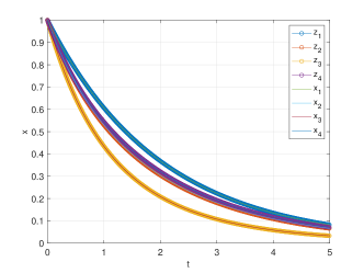
  Figure 1: State trajectories of the original nonlinear system representation (27)-(30) and the Koopman embedding (31).

  • The terms $a$ are already contained in $W_{n}$.

  • We can observe that the power $j_{n}$ decreases by 1 and the powers of $x_{i}$ ($i\in\left\{1,\dots,n-1\right\}$) within $\zeta$ increase by at most $d_{n}$ (which is finite), encoded in terms of $n_{\tilde{j}}$. Applying the same iterations as in case $n=4$, recursively leads to $\mathfrak{D}_{\mathrm{b}}(V_{n+1})\setminus V_{n+1}\subseteq\{x_{1}^{0},\ldots,x_{1}^{n_{1}}\}$ in a finite number of steps.

  • As seen in $n=4$, taking $\frac{\operatorname{d\!}}{\operatorname{d\!}t}\zeta_{j}$ for the terms $c$, leads to a decrease of the orders of $x_{1}^{j_{1}},\ldots,x_{n}^{j_{n}}$ in the terms $\zeta$. By using $V_{n+1}\leftarrow V_{n+1}\cup\mathfrak{D}_{\mathrm{c}}(V_{n+1})$ in a finite number of steps leads to $\mathfrak{D}_{\mathrm{c}}(V_{n+1})\setminus V_{n+1}\subseteq\{x_{n}^{0},\ldots,x_{n}^{n_{n}}\}$. As noted before, the empty set is also a subset and the terms $b$ and $c$ are iterated together.

  Hence, based on case $n$, we know that for $V_{n+1}\leftarrow V_{n+1}\cup\mathfrak{D}_{\mathrm{c}}(V_{n+1})$ taking $W_{n+1}=\{x_{n+1}\}\cup V_{n+1}$ and $\Phi=\mathrm{vec}(\bigcup_{i=1}^{n+1}W_{i})$ will ensure that condition (8a) holds true. This completes the proof.

This shows that for an autonomous polynomial nonlinear system with the dynamics described by (10), there exists a finite dimensional lifting $\Phi$, containing the states and polynomial terms, satisfying $\dot{\Phi}=\frac{\partial\Phi}{\partial x}f\in\mathrm{span}\{\Phi\}$. This implies that there exists a square real matrix $A$ such that $\dot{\Phi}(x)=A\Phi(x)$.

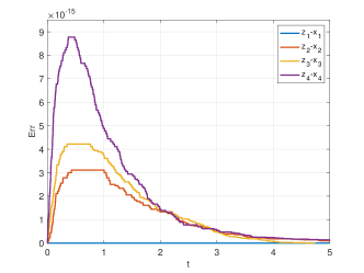
Figure 2: Error between the state trajectories of the original nonlinear system representation (27)-(30) and the Koopman embedding (31).

2.3 Systems with input

Consider the following control affine nonlinear system:

$$\dot{x}=f(x)+g(x)u,$$ (23)

with the autonomous part given by (10) and $g\mathrel{\mathop{\mathchar 58\relax}}\mathbb{R}^{n_{\mathrm{x}}}\rightarrow\mathbb{R}^{n_{\mathrm{x}}\times n_{\mathrm{u}}}$ and $u\in\mathbb{U}\subseteq\mathbb{R}^{n_{\mathrm{u}}}$. To obtain the lifted representation, one can use the sequential method described in (Iacob et al., 2022). First, an exact lifting of the autonomous part is assumed to exist, i.e. conditions (8) hold. Next, the Koopman embedding is computed using the properites of the differential operator. Applying the lifting $\Phi$ and taking the time derivative, one obtains:

$$\begin{split}\dot{\Phi}&=\frac{\partial\Phi}{\partial x}(x)\dot{x}\\ &=\frac{\partial\Phi}{\partial x}(x)f(x)+\frac{\partial\Phi}{\partial x}(x)g(x)u.\end{split}$$ (24)

Using the equivalence of conditions (8b) and (8a), an associated Koopman embedding of (23) is:

$$\dot{\Phi}(x)=A\Phi(x)+B(x)u,$$ (25)

with $B(x)=\frac{\partial\Phi}{\partial x}(x)g(x)$. As described in (Iacob et al., 2022), one can further express (25) as a linear parameter varying (LPV) Koopman representation by introducing a scheduling map $p=\mu(z)$, where $z=\Phi(x)$ and defining $B_{\mathrm{z}}\circ z=B$. Then, the LPV Koopman model is described by:

$$\dot{z}=Az+B_{\mathrm{z}}(p)u,$$ (26)

with $z(0)=\Phi(x(0))$.

3 Example

This section presents the embedding of an example $4$-dimensional system and shows simulation results for both autonomous and input-driven operation.

3.1 Autonomous case

Consider the following $4^{\mathrm{th}}$ order system:

$$\dot{x}_{1} =a_{1}x_{1}$$ (27)

$$\dot{x}_{2} =a_{2}x_{2}+\alpha^{2}_{3}x^{3}_{1}$$ (28)

$$\dot{x}_{3} =a_{3}x_{3}+\alpha^{3}_{11}x_{1}x_{2}+\alpha^{3}_{02}x^{2}_{2}$$ (29)

$$\dot{x}_{4} =a_{4}x_{4}+\alpha^{4}_{111}x_{1}x_{2}x_{3}.$$ (30)

We can apply the procedure discussed in Section 2 per state equation to find the observable functions. The resulting lifting functions are as follows: $W_{1}=\left\{x_{1}\right\}$, $W_{2}=\left\{x_{2},x^{3}_{1}\right\}$, $W_{3}=\left\{x_{3},x_{1}x_{2},x^{2}_{2},x^{4}_{1},x^{3}_{1}x_{2},x^{6}_{1}\right\}$, and $W_{4}=\{x_{4},x_{1}x_{2}x_{3},x^{4}_{1}x_{3},x^{2}_{1}x_{2},x_{1}x^{3}_{2},x^{5}_{1}x_{2},x^{4}_{1}x_{2},x^{8}_{1},x^{7}_{1}x_{2},x^{10}_{1}\}$.
Then, the entire lifting set is $\Phi=\mathrm{vec}(W_{1},W_{2},W_{3},W_{4})$. For easier interpretability, we can write the observables such that: $\Phi(x)=[x_{1}\ x_{2}\ x_{3}\ x_{4}\ \bar{\Phi}_{1}^{\top}\ \bar{\Phi}_{2}^{\top}\ \bar{\Phi}_{3}^{\top}\ \bar{\Phi}_{4}^{\top}]^{\top}$ and $\bar{\Phi}_{i}$ contains the elements of $W_{i}$, in order, without the state $x_{i}$. Performing the derivations as described in the proof, we obtain a finite dimensional Koopman representation of the form:

$$\begin{split}\dot{z}&=Az\\ x&=Cz,\end{split}$$ (31)

with $z(t)=\Phi(x(t))$, $A\in\mathbb{R}^{19\times 19}$ and $C=[I_{4}\;0_{4\times 15}]$. The structure of the state matrix $A$ is detailed in the Appendix. To compare the obtained Koopman representation and the original system description, consider $a_{1}=a_{2}=a_{3}=a_{4}=-0.5$, $\alpha^{2}_{3}=\alpha^{3}_{11}=\alpha^{3}_{02}=\alpha^{4}_{111}=-0.2$ and $x_{0}=[1\;1\;1\;1]^{\top}$. We can obtain solution trajectories of these two representations by a Runge-Kutta $4^{\mathrm{th}}$ order solver. Furthermore, once the initial condition is lifted, i.e. $z(0)=\Phi(x(0))$, the dynamics of the Koopman model are driven forward linearly, as described by (31). The simulation results and solution trajectories are depicted in Fig 1. As it can be observed, there is an exact overlap between the state trajectories of the original system description and the state trajectories obtained from the lifted model ($z_{1\rightarrow 4}$ correspond to $x_{1\rightarrow 4}$). Fig. 2 shows that the obtained error is in the order of magnitude of $10^{-15}$, which can be attributed to numerical artifacts.

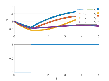
Figure 3: State trajectories of the original nonlinear system detailed in Section 3.2 and the Koopman embedding (32).

3.2 Input-driven case

Consider a control affine nonlinear system (23), with the autonomous part given by the equations (27)-(30) and $g(x)=\left[1\;x_{1}\;x^{2}_{2}\;\sin(x_{3})\right]^{\top}$. Applying the lifting procedure described in Section 2.3, we can derive an exact LPV Koopman model:

$$\begin{split}\dot{z}&=Az+B_{\mathrm{z}}(p)u\\ x&=Cz,\end{split}$$ (32)

with $C=[I_{4}\;0_{4\times 15}]$, $z(t)=\Phi(x(t))$ and $p=z$. Note that the state matrix $A$ coincides with the autonomous case. The explicit form of $B(x)$ (and, in turn, $B_{\mathrm{z}}$) is omitted due to space constraints, but it can be easily computed by multiplying $\frac{\partial\Phi}{\partial x}$ with $g(x)$. The structure of $\frac{\partial\Phi}{\partial x}(x)$ is given in the Appendix. We use the same coefficient values as in the autonomous case and consider a step input. After lifting the initial state $z(0)=\Phi(x(0))$, the dynamics of the Koopman representation are simulated forward in time by (32). Fig. 3 shows the solution trajectories of both the original and the lifted system representations. As in the autonomous case, there is an exact overlap, with the error between the state trajectories being in the order of magnitude of $10^{-15}$, only due to numerical integration errors. This is depicted in Fig. 4.

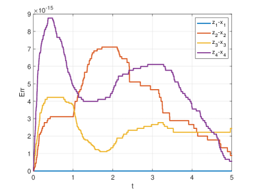
Figure 4: Error between the state trajectories of the original nonlinear system detailed in Section 3.2 and the Koopman embedding (32) under a step input.

4 Conclusion

The present paper shows that a finite, exact Koopman embedding exists for a specific system class and an approach is provided to obtain this embedding. Furthermore, as shown, the step to embed nonlinear systems with input is easily achieved once the autonomous part is lifted. Future work will focus on extending the current system description to a more general class of nonlinear systems.

Appendix A Matrices

$A=\setcounter{MaxMatrixCols}{19}\begin{bmatrix}a_{1}&0&0&0&0&0&0&0&0&0&0&0&0&0&0&0&0&0&0\\ 0&a_{2}&0&0&\alpha^{2}_{3}&0&0&0&0&0&0&0&0&0&0&0&0&0&0\\ 0&0&a_{3}&0&0&\alpha^{3}_{11}&\alpha^{3}_{02}&0&0&0&0&0&0&0&0&0&0&0&0\\ 0&0&0&a_{4}&0&0&0&0&0&0&\alpha^{4}_{111}&0&0&0&0&0&0&0&0\\ 0&0&0&0&3a_{1}&0&0&0&0&0&0&0&0&0&0&0&0&0&0\\ 0&0&0&0&0&a_{1}+a_{2}&0&\alpha^{2}_{3}&0&0&0&0&0&0&0&0&0&0&0\\ 0&0&0&0&0&0&2a_{2}&0&2\alpha^{2}_{3}&0&0&0&0&0&0&0&0&0&0\\ 0&0&0&0&0&0&0&4a_{1}&0&0&0&0&0&0&0&0&0&0&0\\ 0&0&0&0&0&0&0&0&3a_{1}+a_{2}&\alpha^{2}_{3}&0&0&0&0&0&0&0&0&0\\ 0&0&0&0&0&0&0&0&0&6a_{1}&0&0&0&0&0&0&0&0&0\\ 0&0&0&0&0&0&0&0&0&0&a_{1}+a_{2}+a_{3}&\alpha^{2}_{3}&\alpha^{3}_{11}&\alpha^{3}_{02}&0&0&0&0&0\\ 0&0&0&0&0&0&0&0&0&0&0&4a_{1}+a_{3}&0&0&\alpha^{3}_{11}&\alpha^{3}_{02}&0&0&0\\ 0&0&0&0&0&0&0&0&0&0&0&0&2a_{1}+2a_{2}&0&2\alpha^{2}_{3}&0&0&0&0\\ 0&0&0&0&0&0&0&0&0&0&0&0&0&a_{1}+3a_{2}&0&3\alpha^{2}_{3}&0&0&0\\ 0&0&0&0&0&0&0&0&0&0&0&0&0&0&5a_{1}+a_{2}&0&\alpha^{2}_{3}&0&0\\ 0&0&0&0&0&0&0&0&0&0&0&0&0&0&0&4a_{1}+2a_{2}&0&2\alpha^{2}_{3}&0\\ 0&0&0&0&0&0&0&0&0&0&0&0&0&0&0&0&8a_{1}&0&0\\ 0&0&0&0&0&0&0&0&0&0&0&0&0&0&0&0&0&7a_{1}+a_{2}&\alpha^{2}_{3}\\ 0&0&0&0&0&0&0&0&0&0&0&0&0&0&0&0&0&0&10a_{1}\end{bmatrix}$

$\frac{\partial\Phi}{\partial x}(x)=\setcounter{MaxMatrixCols}{19}\begin{bmatrix}1&0&0&0&3x^{2}_{1}&x_{2}&0&4x_{1}^{3}&3x_{1}^{2}x_{2}&6x_{1}^{5}&x_{2}x_{3}&4x_{1}^{3}x_{3}&2x_{1}x_{2}^{2}&x_{2}^{3}&5x_{1}^{4}x_{2}&4x_{1}^{3}x^{2}_{2}&8x_{1}^{7}&7x_{1}^{6}x_{2}&10x_{1}^{9}\\ 0&1&0&0&0&x_{1}&2x_{2}&0&x_{1}^{3}&0&x_{1}x_{3}&0&2x_{1}^{2}x_{2}&3x_{1}x_{2}^{2}&x_{1}^{5}&2x_{1}^{4}x_{2}&0&x_{1}^{7}&0\\ 0&0&1&0&0&0&0&0&0&0&x_{1}x_{2}&x_{1}^{4}&0&0&0&0&0&0&0\\ 0&0&0&1&0&0&0&0&0&0&0&0&0&0&0&0&0&0&0\end{bmatrix}^{\top}$

References

- Abraham and Murphey (2019) Abraham, I. and Murphey, T.D. (2019). Active learning of dynamics for data-driven control using Koopman operators. IEEE Transactions on Robotics, 35(5), 1071–1083.
- Bevanda et al. (2021) Bevanda, P., Sosnowski, S., and Hirche, S. (2021). Koopman operator dynamical models: Learning, analysis and control. Annual Reviews in Control, 52, 197–212.
- Brunton et al. (2022) Brunton, S.L., Budišić, M., Kaiser, E., and Nathan Kutz, J. (2022). Modern Koopman theory for dynamical systems. SIAM Review, 64, 229–340.
- Cisneros et al. (2020) Cisneros, P.S.G., Datar, A., Göttsch, P., and Werner, H. (2020). Data-driven quasi-LPV model predictive control using Koopman operator techniques. 21st IFAC World Congress, 6062–6068.
- Iacob et al. (2021) Iacob, L.C., Beintema, G.I., Schoukens, M., and Tóth, R. (2021). Deep identification of nonlinear systems in Koopman form. 60th IEEE Conference on Decision and Control (CDC), 2288–2293.
- Iacob et al. (2022) Iacob, L.C., Tóth, R., and Schoukens, M. (2022). Koopman form of nonlinear systems with inputs. arXiv:2207.12132, Preprint submitted to Automatica.
- Jouan (2003) Jouan, P. (2003). Immersion of nonlinear systems into linear systems modulo output injection. 42nd IEEE International Conference on Decision and Control (CDC), 1476–1481.
- Khalil (2002) Khalil, H.K. (2002). Nonlinear systems; 3rd ed. Prentice-Hall.
- Klus et al. (2020) Klus, S., Nüske, F., Peitz, S., Niemann, J.H., Clementi, C., and Schütte, C. (2020). Data-driven approximation of the Koopman generator: Model reduction, system identification, and control. Physica D: Nonlinear Phenomena, 406, 132416.
- Kowalski and Steeb (1991) Kowalski, K. and Steeb, W.H. (eds.) (1991). Nonlinear Dynamical Systems and Carleman Linearization. World Scientific.
- Krener and Isidori (1983) Krener, A. and Isidori, A. (1983). Linearization by output injection and nonlinear observers. Systems & Control Letters, 3(1), 47–52.
- Lasota and Mackey (1994) Lasota, A. and Mackey, M.C. (1994). Chaos, Fractals, and Noise: Stochastic Aspects of Dynamics. Springer.
- Lusch et al. (2018) Lusch, B., Nathan Kutz, J., and Brunton, S. (2018). Deep learning for universal linear embeddings of nonlinear dynamics. Nature Communications, 9, 4950.
- Mauroy et al. (2020) Mauroy, A., Mezić, I., and Susuki, Y. (eds.) (2020). The Koopman Operator in Systems and Control: Concepts, Methodologies and Applications. Springer.
- Wang and Jungers (2020) Wang, Z. and Jungers, R. (2020). A data-driven immersion technique for linearization of discrete-time nonlinear systems. 21st IFAC World Congress, 869–874.
- Williams et al. (2015) Williams, M., Kevrekidis, I., and Rowley, C. (2015). A data–driven approximation of the Koopman operator: Extending dynamic mode decomposition. Journal of Nonlinear Science, 25, 1307–1346.