Stochastic and statistical stability of the classical Lorenz flow under perturbations modeling anthropogenic type forcing

Abstract

We review the results obtained in [GMPV] and [GV] on the stochastic and statistical stability of the classical Lorenz flow, where, looking at the Lorenz’63 ODE system as a simple - yet non trivial - model of the atmospheric circulation, the perturbation schemes introduced in these papers are designed to represent the effect of the so called anthropogenic forcing on the dynamics of the atmosphere.

AMS subject classification:

34F05, 93E15.

Keywords and phrases:

Random perturbations of dynamical systems, classical Lorenz flow, random dynamical systems, semi-Markov random evolutions, piecewise deterministic Markov processes, Lorenz’63 model, anthropogenic forcing.

Ethics declaration:

the corresponding author states that there is no conflict of interest.

1 Introduction

1.1 The classical Lorenz flow

Turbulent systems such the atmosphere are usually modeled by flows exhibiting a sensitive dependence on the initial conditions. The behaviour of the trajectories of the system in the phase space for large times is usually numerically very hard to compute and consequently the same computational difficulty affects also the computation of the phase averages of physically relevant observables. A way to overcome this problem is to select a few of these relevant observables under the hypothesis that the statistical properties of the smaller system defined by the evolution of such quantities can capture the important features of the statistical behaviour of the original system [NVKDF].

This turns out to be the case when considering classical Lorenz model, or, in the physics literature, Lorenz’63 model, that is the system of equation

$$\left\{\begin{array}[c]{l}\dot{x}_{1}=-\zeta x_{1}+\zeta x_{2}\\ \dot{x}_{2}=-x_{1}x_{3}+\gamma x_{1}-x_{2}\\ \dot{x}_{3}=x_{1}x_{2}-\beta x_{3}\end{array}\right.\ ,$$ (1)

which was introduced by E. Lorenz in his celebrated paper [Lo] as a simplified yet non trivial model for thermal convection of the atmosphere and, since then, it has been pointed out as the typical real example of a non-hyperbolic three-dimensional flow whose trajectories show a sensitive dependence on initial conditions. More precisely, the classical Lorenz flow, for $\zeta=10,\gamma=28,\beta=8/3,$ has been proved in [Tu], and more recently in [AM], to show the same dynamical features of its ideal counterpart the so called geometric Lorenz flow, introduced in [ABS] and in [GW], which represents the prototype of a three-dimensional flow exhibiting a partially hyperbolic attractor [AP].

1.2 Physical motivations for the study of the stability of the statistical properties of the classical Lorenz flow

The analysis of the stability of the statistical properties of the classical Lorenz flow can provide a theoretical framework for the study of climate changes, in particular those induced by the anthropogenic influence on climate dynamics.

A possible way to study this problem is to add a weak perturbing term to the phase vector field generating the atmospheric flow which model the atmospheric circulation: the so called anthropogenic forcing. Assuming that the atmospheric circulation is described by a model exhibiting a robust singular hyperbolic attractor, as it is the case for the classical Lorenz flow, it has been shown empirically that the effect of the perturbation can possibly affect just the statistical properties of the system [Pa], [CMP]. Therefore, because of its very weak nature (small intensity and slow variability in time), a practical way to measure the impact of the anthropogenic forcing on climate statistics is to look at the extreme value statistics of those particular observables whose evolution may be more sensitive to it [Su]. In the particular case these observables are given by bounded (real valued) functions on the phase space, an effective way to look at their extreme value statistics is to look first at the statistics of their extrema and then eventually to the extreme value statistics of these making use, for example, of the techniques described in [Letal].

1.2.1 Stability of the invariant measure of the classical Lorenz flow

Since $C^{1}$ perturbations of the classical Lorenz vector field admit a $C^{1+\epsilon}$ stable foliation [AM] and since the geometric Lorenz attractor is robust in the $C^{1}$ topology [AP], it is natural to discuss the statistical and the stochastic stability of the classical Lorenz flow under this kind of perturbations.

As a matter of fact, in applications to climate dynamics, when considering the Lorenz’63 flow as a model for the atmospheric circulation, the analysis of the stability of the statistical properties of the unperturbed flow under perturbations of the velocity phase field of this kind can turn out to be a useful tool in the study of the so called anthropogenic climate change [CMP].

2 Statistical stability

Since the SRB measure of the geometric Lorenz flow can be constructed starting from the invariant measure of the one-dimensional map obtained through reduction to the quotient leaf space of the Poincaré map on a two-dimensional manifold transverse to the flow [AP], the statistical stability for the invariant measure of this map implies that of the SRB measure of the unperturbed flow. Results in this direction are given in [AS], [BR] and [GL] where strong statistical stability of the geometric Lorenz flow is analysed.

For what concerns the classical Lorenz flow in [GMPV] it has been shown that the effect of an additive constant perturbation term to the classical Lorenz vector field results into a particular kind of perturbation of the map of the interval describing the evolution of the maxima of the Casimir function for the (+) Lie-Poisson brackets associated to the $so\left(3\right)$ algebra. Moreover, it has been proved that the invariant measures for the perturbed and for the unperturbed 1-$d$ maps of this kind have Lipschitz continuous density and that the unperturbed invariant measure is strongly statistically stable.

More precisely, the vector field (1) has the interesting feature that it can be rewritten as

$$\left\{\begin{array}[c]{l}\dot{y}_{1}=-\zeta y_{1}+\zeta y_{2}\\ \dot{y}_{2}=-y_{1}y_{3}-\gamma y_{1}-y_{2}\\ \dot{y}_{3}=y_{1}y_{2}-\beta y_{3}-\beta\left(\gamma+\zeta\right)\end{array}\right.\ ,$$ (2)

showing the corresponding flow to be generated by the sum of a Hamiltonian $SO\left(3\right)$-invariant field and a gradient field (we refer the reader to [GMPV] and references therein). Therefore, as it has been proved in [GMPV], the invariant measure of the classical Lorenz flow can be constructed starting from the invariant measure of a map of the interval $T,$ whose graph (see fig. 1) looks like that originally computed by Lorenz ([Lo] fig. 4) describing the evolution of the extrema of the first integrals of the associated Hamiltonian flow [PM] such as, for example, the just mentioned Casimir function $C\left(t\right):=\left|Y^{t}\right|^{2},$ where $\left|\cdot\right|$ is the Euclidean norm in $\mathbb{R}^{3}$ and $\left(Y^{t}\ ,t\geq 0\right)$ denotes the flow defined by (2). In this case, denoting by $\phi_{0}$ the vector field defined in (2), since $\dot{C}=\phi_{0}\cdot\nabla C$ and $\ddot{C}=\phi_{0}\cdot\nabla\left(\phi_{0}\cdot\nabla C\right),$ setting, for $\epsilon$ sufficiently small,

$$\mathcal{M}_{\epsilon}:=\left\{\left(y_{1},y_{2},y_{3}\right)\in\mathbb{R}^{3}:\left|y_{1}\right|\leq\epsilon,\left|y_{2}\right|\leq\epsilon,y_{3}\in\left[-\left(\gamma+\zeta\right),\epsilon-\left(\gamma+\zeta\right)\right]\right\}$$ (3)

the Poincaré surface taken into account is

$$\mathcal{M}:=\left\{\left(y_{1},y_{2},y_{3}\right)\in\mathcal{M}_{\epsilon}:\left(\phi_{0}\cdot\nabla C\right)\left(y_{1},y_{2},y_{3}\right)=0,\phi_{0}\cdot\nabla\left(\phi_{0}\cdot\nabla C\right)\left(y_{1},y_{2},y_{3}\right)\leq 0\right\}$$ (4)

Note that $\mathcal{M}$ contains the hyperbolic critical point $c_{0}:=\left(0,0,-\left(\gamma+\zeta\right)\right)$ of $\phi_{0}.$ Denoting by $\bar{T}$ the automorphism of the set of the leaf of the invariant foliation defined by the intersection of the stable manifolds of the flow with $\mathcal{M},T$ is then obtained identifying the leaves of the invariant foliation corresponding to the same values of $C.$

2.1 The Lorenz-like cusp map $T$ and its invariant measure

The local behaviors of the branches of $T$ are ($c$ will denote a positive constant which could take different values from one formula to another):

$$\left\{\begin{array}[c]{l}T(x)=\alpha^{\prime}x+\beta^{\prime}x^{1+\psi}+o(x^{1+\psi});\ x\rightarrow 0^{+}\\ DT(x)=\alpha^{\prime}+cx^{\psi}+o(x^{\psi}),\ \alpha^{\prime}>1;\ \beta^{\prime}>0;\ \psi>1\end{array}\right.\ ,$$ (7)

$$\left\{\begin{array}[c]{l}T(x)=\alpha(1-x)+\tilde{\beta}(1-x)^{1+\kappa}+o((1-x)^{1+\kappa});\ x\rightarrow 1^{-}\\ DT(x)=-\alpha-c(1-x)^{\kappa}+o((1-x)^{\kappa}),\ 0<\alpha<1,\ \tilde{\beta}>0,\ \kappa>1\end{array}\right.\ ,$$ (10)

$$\left\{\begin{array}[c]{l}T(x)=1-A^{\prime}(x_{0}-x)^{B^{\prime}}+o((x_{0}-x)^{B^{\prime}});\ x\rightarrow x_{0}^{-},\ A^{\prime}>0\\ DT(x)=c(x_{0}-x)^{B^{\prime}-1}+o((x_{0}-x)^{B^{\prime}-1}),\ 0<B^{\prime}<1\end{array}\right.\ ,$$ (13)

$$\left\{\begin{array}[c]{l}T(x)=1-A(x-x_{0})^{B}+o((x-x_{0})^{B});\ x\rightarrow x_{0}^{+},\ A>0\\ DT(x)=-c(x-x_{0})^{B-1}+o((x-x_{0})^{B-1}),\ 0<B<1\end{array}\right.\ .$$ (16)

From this we deduce that $T^{-1}$ is $C^{1+\iota},$ for some $\iota\in\left(0,1\right),$ on each open interval $(0,x_{0}),(x_{0},1).$ Indeed, by the result in [AM], the stable foliation for the classical Lorenz flow is $C^{1+\alpha}$ for some $\alpha\in\left(0.278,1\right),$ which means, by (13) and (16), that, for any $x\in(0,x_{0}),T^{\prime}\left(x\right)=\left|x_{0}-x\right|^{1-B^{\prime}}\left[1+G_{1}\left(x\right)\right]$ with $G_{1}\in C^{\alpha B^{\prime}}(0,x_{0})$ and, for any $x\in(x_{0},1),T^{\prime}\left(x\right)=\left|x-x_{0}\right|^{1-B}\left[1+G_{2}\left(x\right)\right]$ with $G_{2}\in C^{\alpha B}(x_{0},1).$ In particular this implies that for any couple of points $x,y$ belonging either to $(0,x_{0})$ or to $(x_{0},1)$

$$|T^{\prime}(x)-T^{\prime}(y)|\leq C_{h}\left|T^{\prime}(x)\right|\left|T^{\prime}(y)\right|\left|x-y\right|^{\iota}\ ,$$ (17)

where $\iota\in(0,1-B^{\ast}],$ with $B^{\ast}:=B\vee B^{\prime},$ and the constant $C_{h}$ is independent of the location of $x$ and $y.$

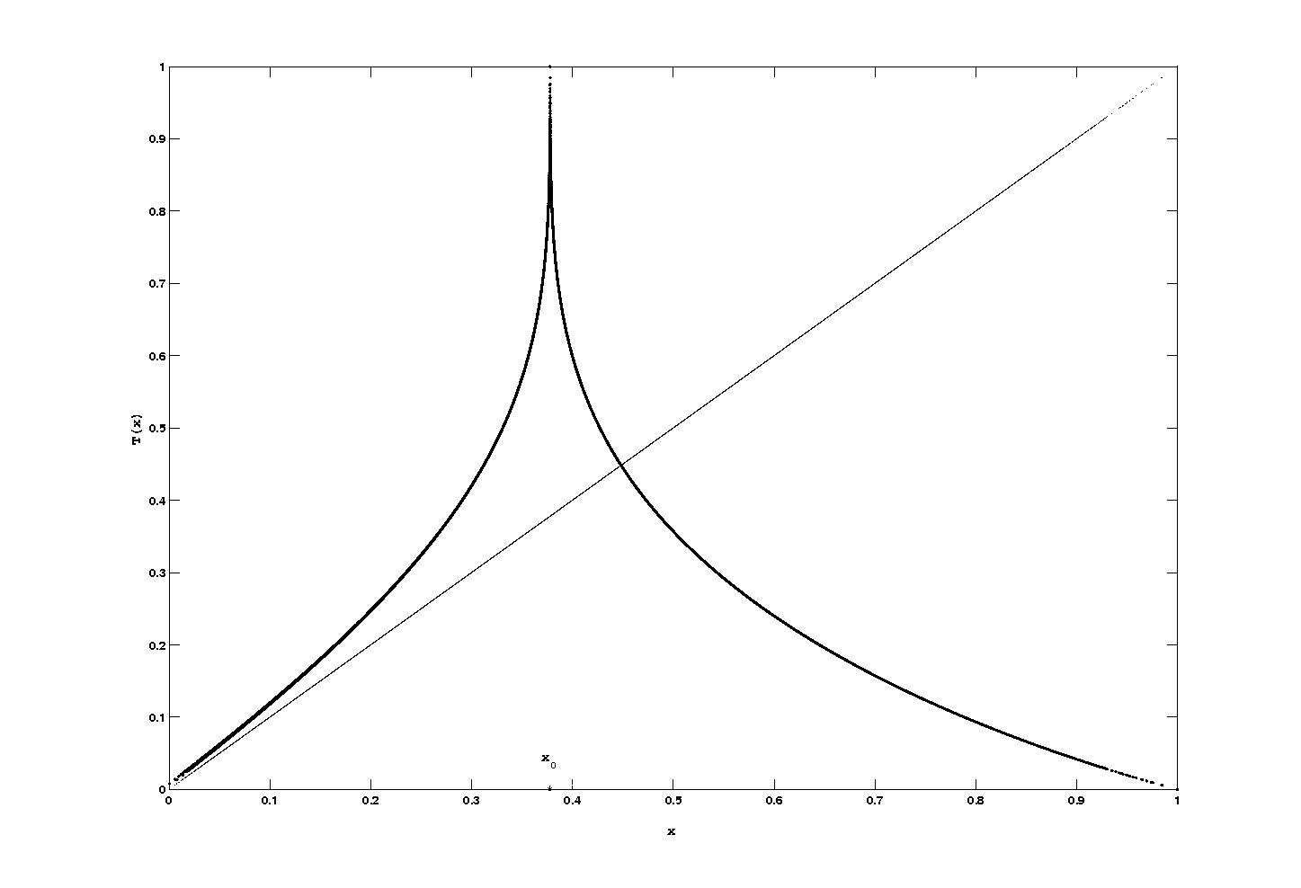
Figure 1: Normalized Lorenz cusp map for the Casimir maxima

Proposition 1

The density $\rho$ of the invariant measure $\mu$ is Lipschitz continuous and bounded over the intervals $[0,1]$. Moreover,

$$\lim_{x\rightarrow 0^{+}}\rho(x)=\lim_{x\rightarrow 1^{-}}\rho(x)=0\ .$$ (18)

Sketch of the proof. Let us set: $a_{0}:=T_{2}^{-1}x_{0};$ $a_{0}^{\prime}:=T_{1}^{-1}x_{0};$ $a_{p}^{\prime}=T_{1}^{-p}a_{0}^{\prime};$ $a_{p}=T_{2}^{-1}T_{1}^{-(p-1)}a_{0}^{\prime},$ $p\geq 1.$ We also define the sequences $\{b_{p}\}_{p\geq 1}\subset(x_{0},a_{0})$ and $\{b_{p}^{\prime}\}_{p\geq 1}\subset(a_{0}^{\prime},x_{0})$ as $Tb_{p}^{\prime}=Tb_{p}=a_{p-1}.$ Hence, we can induce on $I:=(a_{0}^{\prime},a_{0})\backslash\{x_{0}\}$ and to replace the action of $T$ on $I$ with that of the first return map $T_{I}$ into $I$ and prove that the systems $(I,T_{I})$ will admit an absolutely continuous invariant measure $\mu_{I}$ which is in particular equivalent to the Lebesgue measure with a density $\rho_{I}$ bounded from below and from above. To do this, following [CHMV], we also need to induce over the open sets $(a_{n}^{\prime},a_{n-1}^{\prime})$ and $(a_{n},a_{n+1}),n>1,$ simply denoted in the following as the rectangles $I_{n},$ provided we show that the induced maps are aperiodic uniformly expanding Markov maps with bounded distortion on each set with prescribed return time. On the sets $I_{n}$ the first return map $T_{I_{n}}$ is Bernoulli, while the aperiodicity condition on $I$ follows by direct inspection of the graph of the first return map $T_{I}:I\circlearrowleft$ showing that it maps: $(a_{0}^{\prime},b_{1}^{\prime})$ onto $(x_{0},a_{0});$ the intervals $(b_{l}^{\prime},b_{l+1}^{\prime}),\ l\geq 1,$ onto the interval $(a_{0}^{\prime},x_{0});$ the interval $(b_{1},a_{0})$ onto $(x_{0},a_{0})$ and finally the intervals $(b_{l+1},b_{l}),\ l\geq 1$ onto $(a_{0}^{\prime},x_{0}).$ The proof of the boundedness of the distortion is analogous to that given in Proposition 3 of [CHMV] and rely on the proof that the first return maps are uniformly expanding. In particular, in the initial formula (5) in [CHMV] we need now to replace the term $\left|\frac{D^{2}T(\xi)}{DT(\xi)}\right||T^{q}\left(x\right)-T^{q}\left(y\right)|,$ where $\xi$ is a point between $T^{q}\left(x\right)$ and $T^{q}\left(y\right),$ with $\frac{1}{|DT(\xi)|}C_{h}|DT(T^{q}\left(x\right))||DT(T^{q}\left(y\right))||T^{q}\left(x\right)-T^{q}\left(y\right)|^{\iota}$ which is smaller than $C_{h}\left(|DT(T^{q}\left(x\right))|\vee|DT(T^{q}\left(y\right))|\right)|T^{q}\left(x\right)-T^{q}\left(y\right)|^{\iota}$ by monotonicity of $\left|DT\right|.$ The key estimate (11) in [CHMV] will reduce in our case to the bound of the quantity $\sup_{\xi\in[b_{i+1},b_{i}]}|DT\left(\xi\right)||b_{i}-b_{i+1}|.$ By using for $DT$ the expressions given in the formulas (13) and (16), and for the $b_{i}$ the scaling $(x_{0}-b_{p}^{\prime})\sim\frac{c}{\left(\alpha^{\prime}\right)^{\frac{p}{B^{\prime}}}};\ (b_{p}-x_{0})\sim\frac{c}{\left(\alpha^{\prime}\right)^{\frac{p}{B}}}$ (see formula (75) of [GMPV]) we immediately get that the above quantity is of order $\frac{1}{(\alpha^{\prime})^{i}},$ which is enough to pursue the argument about the estimate of the distortion presented in [CHMV].

The invariant measure $\mu_{I}$ for the induced map $T_{I}$ is related to the invariant measure $\mu$ over the whole interval by the Pianigiani formula

$$\mu(B)=C_{r}\sum_{i}\sum_{j=0}^{\tau_{i}-1}\mu_{I}(T^{-j}(B)\cap Z_{i})$$ (19)

where $B$ is any Borel set in $[0,1]$ and the first sum runs over the cylinders $Z_{i}$

$$Z_{1} =(a_{0}^{\prime},b_{1}^{\prime})\cup(b_{1},a_{0})$$ (20)

$$Z_{i} =(b_{i-1}^{\prime},b_{i}^{\prime})\cup(b_{i},b_{i-1})\quad i\geq 2\ ,$$ (21)

with prescribed first return time $\tau_{i}$ and whose union gives $I.$ The normalizing constant $C_{r}=\mu(I)$ satisfies $1=C_{r}\sum_{i}\tau_{i}\mu_{I}(Z_{i}).$ This immediately implies that by calling $\hat{\rho}$ the density of $\mu_{I}$ we have that $\rho(x)=C_{r}\hat{\rho}(x)$ for Lebesgue almost every $x\in I$ and therefore $\rho$ can be extended to a Lipschitz continuous function on $I$ as $\hat{\rho}.$   

Anyway, we remark that the existence of an invariant measure for $T$ follows also by combining Theorem 2 in [Pi2] and the results in section 4.2 of [Bu] since one can check by direct computation that the map $T:=W\circ T\circ W^{-1},$ where $W$ is the distribution function associated to the probability measure on $\left(\left[0,1\right],\mathcal{B}\left(\left[0,1\right]\right)\right)$ with density

$$\left[0,1\right]\ni x\longmapsto W^{\prime}\left(x\right):=N_{\bar{\gamma},\bar{\beta}}e^{-\bar{\gamma}x}x^{\bar{\beta}}\left(1-x\right)^{\bar{\beta}}$$ (22)

(see formulas (83) and (84) in [GMPV]) for suitably chosen parameters $\bar{\gamma},\bar{\beta}>0,$ is such that $\inf\left|\overline{T}^{\prime}\right|>1.$

2.1.1 Statistical stability of $T$

Let us denote by $\lambda$ the Lebesgue measure on $\left(\mathbb{R},\mathcal{B}\left(\mathbb{R}\right)\right)$ and by $T_{\epsilon}$ the perturbed map. We show that under the following assumptions the density $\rho_{\epsilon}$ of the perturbed measure will converge to the density $\rho$ of the unperturbed one in the $L_{\lambda}^{1}$ norm.

• $T_{\epsilon}$ is a Markov map of the unit interval which is one-to-one and onto on the intervals $[0,x_{\epsilon,0})$ and $(x_{\epsilon,0},1],$ convex on both sides and of class $C^{1+\iota_{\epsilon}}$ on the open interval $(0,x_{\epsilon,0})\cup(x_{\epsilon,0},1).$

• Let $\left\|\cdot\right\|_{0}$ denotes the $C^{0}$-norm on the unit interval, then

  $$\lim_{\epsilon\rightarrow 0}\left\|T_{\epsilon}-T\right\|_{0}=0\ .$$ (23)

  Moreover, $\forall x\in[0,1],\ x\neq x_{0},$ we can find $\epsilon(x)$ such that,$\forall\epsilon<\epsilon(x),\ DT_{\epsilon}$ exists and is finite and we have

  $$\lim_{\epsilon\rightarrow 0}DT_{\epsilon}(x)=DT(x)\ .$$ (24)

  Furthermore,

  $$\lim_{x\rightarrow x_{0}^{+}}\lim_{\epsilon\rightarrow 0}\frac{DT_{\epsilon}(x)}{DT(x)}=\lim_{x\rightarrow x_{0}^{-}}\lim_{\epsilon\rightarrow 0}\frac{DT_{\epsilon}(x)}{DT(x)}=1\ .$$ (25)

• Let us denote by $C_{h,\epsilon}$ and $\iota_{\epsilon}$ respectively the Hölder constant and the Hölder exponent for the derivative of $T_{\epsilon}$ on the open interval $(0,x_{\epsilon,0})\cap(x_{\epsilon,0},1);$ namely: $|DT_{\epsilon}(x)-DT_{\epsilon}(y)|\leq C_{h,\epsilon}|x-y|^{\iota_{\epsilon}}$ for any $x,y$ either in $(0,x_{\epsilon,0})$ or in $(x_{\epsilon,0},1).$ We assume $C_{h,\epsilon}$ and $\iota_{\epsilon}$ to converge to the corresponding quantities for $T$ in the limit $\epsilon\rightarrow 0.$

• Let us set $d_{(\epsilon,1,0)}:=\inf_{(b_{\epsilon,1},a_{\epsilon,0})}|DT_{\epsilon}(x)|.$ We assume $d_{(\epsilon,1,0)}>1$ and that there exists a constant $d_{c}$ and $\epsilon_{c}=\epsilon\left(d_{c}\right)$ such that,
  $\forall\epsilon<\epsilon_{c},\ |d_{(1,0)}-d_{(\epsilon,1,0)}|<d_{c}.$

Examples of $T_{\epsilon}$ are plotted in fig. 2 (see also fig. 3 in [GMPV]). We remark that these realizations of the perturbed map $T_{\epsilon}$ occur when a constant perturbing vector field of order $\epsilon$ is added to (2), just as it has been empirically shown in the physics literature (see e.g. [CMP]) it turns out to be the case when considering the effect on the atmospheric circulation of greenhouse gases. Clearly under these assumptions the map $T_{\epsilon}$ will admit a unique absolutely continuous invariant measure with density $\rho_{\epsilon}.$ This density will be related to the invariant density $\hat{\rho}_{\epsilon}$ of the first return map $F_{\epsilon}$ on $I_{\epsilon}$ by the formula

$$\rho_{\epsilon}(x)=C_{\epsilon,r}\sum_{m=2}^{\infty}\sum_{l=1,2}\frac{\hat{\rho}(T_{\epsilon,l}^{-1}T_{\epsilon,2}^{-1}T_{\epsilon,1}^{-(m-2)}x)}{|DT_{\epsilon}^{m}(T_{\epsilon,l}^{-1}T_{\epsilon,2}^{-1}T_{\epsilon,1}^{-(m-2)}x)|}$$ (26)

for $\lambda$-a.e. $x\in(a_{n}^{\prime},a_{n-1}^{\prime})$ uniformly in $n\geq 1$ (see [GMPV] formula (70)). Moreover, we will have that the convergence of the perturbed map to the unperturbed one in the $C^{0}$ topology will imply that the density of the absolutely continuous invariant perturbed measure converges to the density of the unperturbed measure in the $L_{\lambda}^{1}$ norm.

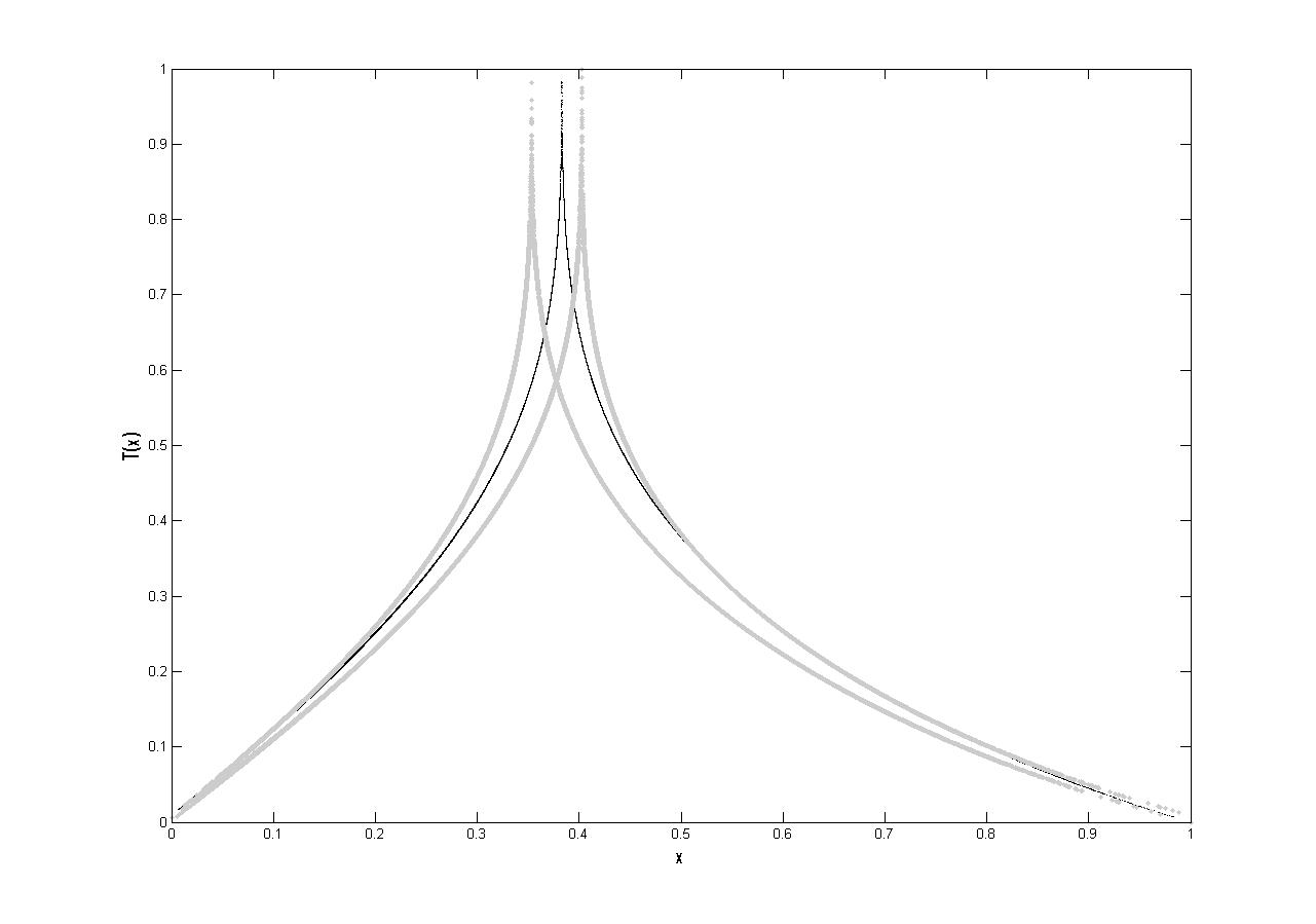
Figure 2: experimental plots of the unperturbed map $T$ (in black) and of its perturbations (in grey).

Proposition 2

$$\lim_{\epsilon\rightarrow 0^{+}}\left\|\rho-\rho_{\epsilon}\right\|_{L_{\lambda}^{1}}=0\,.$$ (27)

The proof of this result make use of induction but, in order to preserve the Markov structure of the first return map, we need to compare the perturbed and the unperturbed first return maps on different induction subsets. Therefore, the difficulty in following this approach arises in the comparison of the Perron-Frobenius operator associated to the induced perturbed system $\left(I_{\epsilon},T_{I_{\epsilon}}\right)$ with the Perron-Frobenius operator associated with the unperturbed one $\left(I,T_{I}\right),$ which will now be defined on different functional spaces. We defer the reader to [GMPV] for the details.

3 Stochastic stability

3.1 Random perturbations

Random perturbations of the classical Lorenz flow have been studied in the framework of stochastic differential equations [Sc], [CSG], [Ke] (see also [Ar] and reference therein). The main interest of these studies was bifurcation theory and the existence and the characterization of the random attractor. The existence of the stationary measure for this stochastic version of the system of equations given in (2) is proved in [Ke].

Stochastic stability under diffusive type perturbations has been studied in [Ki] for the geometric Lorenz flow and in [Me] for the contracting Lorenz flow.

In [GV] we introduced a random perturbation of the Lorenz’63 flow which, being of impulsive nature, differ from diffusion-type perturbations.

• For any realization of the noise $\eta\in\left[-\varepsilon,\varepsilon\right],$ we consider a flow $\left(\Phi_{\eta}^{t},t\geq 0\right)$ generated by the phase vector field $\phi_{\eta}$ belonging to a sufficiently small neighborhood of the classical Lorenz one in the $C^{1}$ topology.

• For $\varepsilon$ small enough, the realizations of the perturbed phase vector field $\phi_{\eta}$ can be chosen such that there exists an open neighborhood $U$ of the unperturbed attractor in $\mathbb{R}^{3},$ independent of the noise parameter $\eta,$ containing the attractor of any realization of $\phi_{\eta}$

• The perturbation acts modifying the phase velocity field of the system at the ring of a random clock $\mathfrak{t}$

This procedure defines a semi-Markov random evolution (sMRE) [KS], in fact a piecewise deterministic Markov process (PDMP) [Da].

To guarantee the existence of an invariant measure for a stochastic process of this kind its imbedded renewal process must satisfy some minimal requirements. In particular, when the evolution of the system is started outside $U$ the trajectories of the system must enter in $U$ with probability one and when the initial condition belongs to $U$ the expected number of modifications of the phase vector field in a finite interval of time must be finite. Furthermore, to make sure that the imbedded Markov chain has a stationary measure, it has to satisfy some requirement such as for example to admit a Ljapunov function (see e.g. [MT]). Therefore, we assume that $\varepsilon$ sufficiently small so that a given Poincaré section $\mathcal{M}$ for the unperturbed flow is also transversal to any realization of the perturbed one and allow changes in the phase velocity field of (2) just at the crossing of $\mathcal{M}.$ Namely, let $\hat{\tau}_{\eta}:U\rightarrow\mathbb{R}$ and $\tau_{\eta}:\mathcal{M}\rightarrow\mathbb{R}$ be respectively the hitting time of $\mathcal{M}$ and the return time map on $\mathcal{M}$ for $\left(\Phi_{\eta}^{t},t\geq 0\right).$ If $\eta$ is sampled according to a given law $\lambda_{\varepsilon}$ supported on $\left[-\varepsilon,\varepsilon\right],$ the sequence $\left\{\mathfrak{x}_{i}\right\}_{i\geq 0}$ such that $\mathfrak{x}_{0}\in\mathcal{M}$ and, for $i\geq 0,\mathfrak{x}_{i+1}:=\Phi_{\eta}^{\tau_{\eta}\left(\mathfrak{x}_{i}\right)}\left(\mathfrak{x}_{i}\right)$ is a homogeneous Markov chain on $\mathcal{M}$ with transition probability measure

$$\mathbb{P}\left\{\mathfrak{x}_{1}\in dz|\mathfrak{x}_{0}\right\}=\lambda_{\varepsilon}\left\{\eta\in\left[-1,1\right]:R_{\eta}\left(\mathfrak{x}_{0}\right)\in dz\right\}\ .$$ (28)

Considering the collection of sequences of i.i.d.r.v’s $\left\{\eta_{i}\right\}_{i\geq 0}$ distributed according to $\lambda_{\varepsilon},$ we define the random sequence $\left\{\sigma_{n}\right\}_{n\geq 1}\in\mathbb{R}^{\mathbb{N}}$ such that $\sigma_{n}:=\sum_{i=0}^{n-1}\tau_{\eta_{i-1}}\left(\mathfrak{x}_{i-1}\right),n\geq 1.$ Then, it is easily checked that the sequence $\left\{\left(\mathfrak{x}_{n},\mathbf{t}_{n}\right)\right\}_{n\geq 0}$ such that $\mathbf{t}_{0}:=\sigma_{1}$ and, for $n\geq 0,\mathbf{t}_{n}:=\sigma_{n+1}-\sigma_{n}$ is a Markov renewal process (MRP) [As], [KS]. Therefore, denoting by $\left(\mathbf{N}_{t},t\geq 0\right),$ such that $\mathbf{N}_{0}:=0$ and $\mathbf{N}_{t}:=\sum_{n\geq 0}\mathbf{1}_{\left[0,t\right]}\left(\sigma_{n}\right),$ the associated counting process and defining:

• $\left(\mathfrak{x}_{t},t\geq 0\right),$ such that $\mathfrak{x}_{t}:=\mathfrak{x}_{\mathbf{N}_{t}},$ the associated semi-Markov process;

• $\left(\mathfrak{l}_{t},t\geq 0\right),$ such that $\mathfrak{l}_{t}:=t-\sigma_{\mathbf{N}_{t}},$ the age (residual life) of the MRP;

• $\left(\eta_{t},t\geq 0\right)$ such that $\eta_{t}:=\eta_{\mathbf{N}_{t}},$

setting $\sigma_{0}:=\hat{\tau}_{\eta},$ we introduce the random process $\left(\mathfrak{u}_{t},t\geq 0\right),$ such that

$$\mathfrak{u}_{t}\left(y_{0}\right):=\left\{\begin{array}[c]{ll}\Phi_{\eta}^{t}\left(y_{0}\right)\mathbf{1}_{[0,\sigma_{0}\left(y_{0}\right))}\left(t\right)+\mathbf{1}_{\left\{\Phi_{\eta}^{\sigma_{0}\left(y_{0}\right)}\left(y_{0}\right)\right\}}\left(\mathfrak{x}_{0}\right)\Phi_{\eta_{\mathbf{N}_{t-\sigma_{0}\left(y_{0}\right)}}}^{\mathfrak{l}_{t-\sigma_{0}\left(y_{0}\right)}}\circ\mathfrak{x}_{t-\sigma_{0}\left(y_{0}\right)}&y_{0}\in U\backslash\mathcal{M}\\ \mathbf{1}_{\left\{y_{0}\right\}}\left(\mathfrak{x}_{0}\right)\Phi_{\eta_{\mathbf{N}_{t}}}^{\mathfrak{l}_{t}}\circ\mathfrak{x}_{t}&y_{0}\in\mathcal{M}\end{array}\right.\ ,$$ (29)

describes the system evolution started at $y_{0}\in U$ (Fig.3).

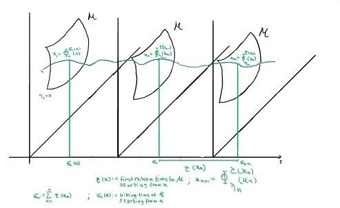
Figure 3: perturbation scheme

We prove:

Theorem 3

There exists a measure $\mu_{\varepsilon}$ on the measurable space $\left(U,\mathcal{B}\left(U\right)\right),$ with $\mathcal{B}\left(U\right)$ the trace $\sigma$algebra of the Borel $\sigma$algebra of $\mathbb{R}^{3},$ such that, for any bounded real-valued measurable function $f$ on $U,$

$$\lim_{T\rightarrow\infty}\frac{1}{T}\int_{0}^{T}dtf\circ\mathfrak{u}_{t}=\mu_{\varepsilon}\left(f\right)$$ (30)

and

$$\lim_{\varepsilon\downarrow 0}\mu_{\varepsilon}\left(f\right)=\mu_{0}\left(f\right)\ ,$$ (31)

where $\mu_{0}$ is the physical measure of the classical Lorenz flow.

In other words, we show that we can recover the physical measure of the unperturbed flow as weak limit, as the intensity of the perturbation vanishes, of the measure on the phase space of the system obtained by looking at the law of large numbers for cumulative processes defined as the integral over $\left[0,t\right]$ of functionals on the path space of the stationary process representing the perturbed system’s dynamics. Therefore, we will reduce ourselves to prove that the imbedded Markov chain driving the random process that describes the evolution of the system is stationary, that its stationary (invariant) measure is unique and that it will converge weakly to the invariant measure of the unperturbed Poincaré map corresponding to $\mathcal{M}.$ To prove existence and uniqueness of the stationary initial distribution of a Markov chain with uncountable state space is not an easy task in general (we refer the reader to [MT] for an account on this subject). To overcome this difficulty we can take advantage of the representation of the Markov chain $\left\{\mathfrak{x}_{n}\right\}_{n\geq 0}$ as a Random Dynamical System (RDS) and consequently make use of the skew-product structure of the first return maps $R_{\eta}.$ Furthermore, we can also show that the trajectories of the PDMP (29) are conjugated to those of a suspension semi-flow over a RDS defined on $\left\{\mathfrak{x}_{n}\right\}_{n\geq 0}$ with roof function defined in terms of the realizations of the r.v. describing the return time on $\mathcal{M}.$ This led us to give a proof of Theorem 3 directly in the framework of the theory of dynamical systems.

However, if the perturbation of the phase velocity field in (2) is given by the addition to the unperturbed one $\phi_{0}$ of a small constant term, namely $\phi_{\eta}:=\phi_{0}+\eta H,H\in\mathbb{S}^{2},$ the proof of the existence of an invariant measure for the unperturbed Poincaré map will follow a more direct strategy.

3.1.1 Proof of Theorem 3

The process $\left(\mathfrak{v}_{t},t\geq 0\right)$ such that $\mathfrak{v}_{t}:=\left(\mathfrak{x}_{t},\mathbf{N}_{t},\mathfrak{l}_{t}\right)$ is a homogeneous Markov process and so is the process $\left(\mathfrak{w}_{t},t\geq 0\right)$ such that $\mathfrak{w}_{t}:=\left(\mathfrak{x}_{t},\mathfrak{l}_{t}\right).$ Moreover $\overline{\mathcal{F}}_{t}^{\mathfrak{w}}\subseteq\overline{\mathcal{F}}_{t}^{\mathfrak{v}}$ and it follows from [Da] Theorem A2.2 that these $\sigma$algebras are both right continuous.

Assume for the moment that the Markov chain $\left\{\mathfrak{x}_{n}\right\}_{n\in\mathbb{Z}^{+}}$ is Harris recurrent (see e.g. [MT] or [H-LL]). By formula (3.9) in [Al] Corollary 1, (see also [Al] Theorem 3) we have that for any $x\in\mathcal{M},v\geq 0$ and any measurable set $A\subseteq\mathcal{M},$

$$\lim_{t\rightarrow\infty}\mathbb{P}\left\{\mathfrak{x}_{t}\in A,\mathfrak{l}_{t}>z|\mathfrak{x}_{0}=x,\mathfrak{l}_{0}=v\right\}=\frac{\int_{\mathcal{M}}\nu_{2}^{\varepsilon}\left(dx\right)\left[\mathbf{1}_{A}\left(x\right)\int_{z}^{\infty}ds\left(1-F_{\tau}^{\varepsilon}\left(s;x\right)\right)\right]}{\int_{\mathcal{M}}\nu_{2}^{\varepsilon}\left(dx\right)\left[\int_{0}^{\infty}ds\left(1-F_{\tau}^{\varepsilon}\left(s;x\right)\right)\right]}\;,\;\mathbb{P}\text{-a.s.\ ,}$$ (32)

where for any $x\in\mathcal{M},t\geq 0,$

$$F_{\tau}^{\varepsilon}\left(t;x\right):=\mathbb{P}\left\{\omega\in\Omega:\mathbf{t}\left(x,\omega\right)\leq t\right\}=\lambda_{\varepsilon}\left\{\eta\in\left[-1,1\right]:\tau_{\eta}\left(x\right)\leq t\right\}$$ (33)

and $\nu_{2}^{\varepsilon}$ is the stationary measure for $\left\{\mathfrak{x}_{n}\right\}_{n\in\mathbb{Z}^{+}}.$ The following result, the proof of which is deferred to [GV], defines the physical measure of (29).

Proposition 4

For any bounded measurable function $f$ on $U$ and any $y_{0}\in U,$

$$\lim_{t\rightarrow\infty}\frac{1}{t}\int_{0}^{t}dsf\circ\mathfrak{u}_{s}\left(y_{0}\right)=\frac{\int_{\left[-1,1\right]}\lambda_{\varepsilon}\left(d\eta\right)\int_{\mathcal{M}}\nu_{2}^{\varepsilon}\left(dx\right)\int_{0}^{\tau_{\eta}\left(x\right)}dsf\left(\Phi_{\eta}^{s}\left(x\right)\right)}{\int_{\mathcal{M}}\nu_{2}^{\varepsilon}\left(dx\right)\left[\int_{0}^{\infty}ds\left(1-F_{\tau}^{\varepsilon}\left(s;x\right)\right)\right]}\;,\;\mathbb{P}\text{-a.s.}$$ (34)

Therefore, defining

$$\mu_{\varepsilon}\left(f\right):=\frac{\int_{\left[-1,1\right]}\lambda_{\varepsilon}\left(d\eta\right)\int_{\mathcal{M}}\nu_{2}^{\varepsilon}\left(dx\right)\int_{0}^{\tau_{\eta}\left(x\right)}ds}{\int\nu_{2}^{\varepsilon}\left(dx\right)\left[\int_{0}^{\infty}ds\left(1-F_{\tau}^{\varepsilon}\left(s;x\right)\right)\right]}f\circ\Phi_{\eta}^{s}\left(x\right)\ ,$$ (35)

assuming the stochastic stability of the invariant measure $\mu_{R_{0}}$ for the unperturbed Poincaré map $R_{0},$ namely the weak convergence of $\nu_{2}^{\varepsilon}$ to $\mu_{R_{0}}$ as $\varepsilon\downarrow 0,$ since for any bounded real-valued measurable function $\varphi$ on $\mathcal{M}\times\mathbb{R}^{+},$

$$\lim_{\varepsilon\rightarrow 0}\frac{1}{\nu_{2}^{\varepsilon}\left[\int_{0}^{\infty}ds\left(1-F_{\tau}^{\varepsilon}\left(s;\cdot\right)\right)\right]}\int_{\mathcal{M}}\nu_{2}^{\varepsilon}\left(dx\right)\int_{0}^{\tau_{\eta}\left(x\right)}ds\varphi\left(x,s\right)=$$ (36)

$$=\int_{\mathcal{M}}\mu_{R_{0}}\left(dx\right)\int_{0}^{\tau_{0}\left(x\right)}ds\frac{1}{\mu_{R_{0}}\left[\tau_{0}\right]}\varphi\left(x,s\right)=\mu_{S_{0}}\left(\varphi\right)\ ,$$

where $S_{0}$ is the suspension flow over $R_{0}$ with roof function $\tau_{0},$ we get

$$\lim_{\varepsilon\rightarrow 0}\mu_{\varepsilon}\left(f\right)=\mu_{S_{0}}\left(f\circ\Phi_{0}^{\cdot}\right)=\int_{\mathcal{M}}\mu_{R_{0}}\left(dx\right)\int_{0}^{\tau_{0}\left(x\right)}ds\frac{1}{\mu_{R_{0}}\left[\tau_{0}\right]}f\circ\Phi_{0}^{s}\left(x\right)\ ,$$ (37)

that is the proof of the following result.

Theorem 5

If $\nu_{2}^{\varepsilon}$ weakly converges to $\mu_{R_{0}},$ then $\mu_{\varepsilon}$ weakly converges to the unperturbed physical measure.

Therefore we are left with the proof of the existence and uniqueness of $\nu_{2}^{\varepsilon}$ and of its weak convergence to $\mu_{R_{0}}$ in the limit $\varepsilon\downarrow 0.$ As we have already outlined, this can be done making use of the representation of the Markov chain $\left\{\mathfrak{x}_{n}\right\}_{n\in\mathbb{Z}^{+}}$ as RDS.

Remark 6

We remark that the Harris recurrence property, which once proven to hold for $\left\{\mathfrak{x}_{n}\right\}_{n\in\mathbb{Z}^{+}}$ entail the existence and uniqueness of $\nu_{2}^{\varepsilon},$ will hold for the Markov chain described in step 2 below, since by construction (see assumption A5 below) its transition probabilities satisfy condition (i) of Theorem 3.1 in [H-LL]. This in turn will imply the SLLN for sequences of r.v.’s of the form $\left\{f\circ\mathfrak{x}_{n}\right\}_{n\in\mathbb{Z}^{+}},$ for any $f\in L^{1}\left(\nu_{2}^{\varepsilon}\right),$ hence the Harris recurrence property for $\left\{\mathfrak{x}_{n}\right\}_{n\in\mathbb{Z}^{+}},$ by Remark 3 and Corollary 4, in view of Proposition 2, in [GV].

We also remark that in the proof of Theorem 3 carried on by following the steps 1 to 8 listed below we do not need to take in to account the Harris recurrence property of the driving Markov chain $\left\{\mathfrak{x}_{n}\right\}_{n\in\mathbb{Z}^{+}}$ of the PDMP (29).

On the other hand, proceeding as in [Op] is possible to prove the invariance principle (functional CLT) and almost sure invariance principle (almost sure functional CLT) for a class of additive functionals of the semi-Markov process $\left(\mathfrak{x}_{t},t\geq 0\right)$ and as a direct consequence for a class of additive functionals of the PDMP (29). We stress that, in our case, assumption A2 in [Op] can be replaced by the requirement of the existence and uniqueness of $\nu_{2}^{\varepsilon}.$

In the special case of random perturbations of $\left(\Phi_{0}^{t},t\geq 0\right)$ realized by the addition to the unperturbed phase vector field of a constant random term, namely

$$\phi_{\eta}:=\phi_{0}+\eta H\ ,\;\eta\in spt\lambda_{\varepsilon}\ ,$$ (38)

with $H\in\mathbb{R}^{3},$ we can take a step forward w.r.t. the problem of showing the existence of an invariant measure for $\left\{\mathfrak{x}_{n}\right\}_{n\in\mathbb{Z}^{+}}.$ Indeed, it has been shown in [PP] that the Casimir function defined in section 2 is a Lyapunov function for the ODE system defined by $\phi_{\eta},$ namely, for any realization of the noise $\eta\in spt\lambda_{\varepsilon},$

$$\left(C\circ\Phi_{\eta}^{t}\right)\left(u\right)\leq C\left(u\right)e^{-t\min\left(1,\zeta,\beta\right)}+\frac{\left\|H_{\eta}\right\|^{2}}{\left(\min\left(1,\zeta,\beta\right)\right)^{2}}\left(1+e^{-t\min\left(1,\zeta,\beta\right)}\right)\ ,$$

where $\mathbb{R}^{3}\ni u\longmapsto C\left(u\right):=\left\langle u,u\right\rangle=\left\|u\right\|^{2}\in\mathbb{R}^{+}$ and $H_{\eta}:=\eta H+H_{0}\in\mathbb{R}^{3},$ with $H_{0}:=\left(0,0,-\beta\left(\zeta+\gamma\right)\right).$

Hence, choosing $t=\tau_{\eta}\left(u\right)$ we obtain

$$C\circ R_{\eta}\left(u\right)\leq a_{\varepsilon}C\left(u\right)+K_{\varepsilon}\left(1+a_{\varepsilon}\right)\ ,$$ (39)

where

$$a_{\varepsilon} :=e^{-\min\left(1,\zeta,\beta\right)\inf_{\eta\in spt\lambda_{\varepsilon}}\inf_{u\in\mathcal{M}}\tau_{\eta}\left(u\right)}\in\left(0,1\right)\;,$$ (40)

$$K_{\varepsilon} :=\frac{\sup_{\eta\in spt\lambda_{\varepsilon}}\left\|H_{\eta}\right\|^{2}}{\left(\min\left(1,\zeta,\beta\right)\right)^{2}}>0\;.$$ (41)

Moreover, for any $\varsigma>0,$

$$\left(1+\varsigma C\right)\circ R_{\eta}\left(u\right) \leq 1+\varsigma a_{\varepsilon}C\left(u\right)+\varsigma K_{\varepsilon}\left(1+a_{\varepsilon}\right)$$ (42)

$$=a_{\varepsilon}\left(1+\varsigma C\left(u\right)\right)+\bar{K}_{\varepsilon}\ ,$$

where $\bar{K}_{\varepsilon}:=\left(1-a_{\varepsilon}\right)+\varsigma K_{\varepsilon}\left(1+a_{\varepsilon}\right),$ which entails for the transition operator $P_{R}$ of the Markov chain $\left\{\mathfrak{x}_{n}\right\}_{n\in\mathbb{Z}^{+}}$

$$C_{b}\left(\mathcal{M}\right)\ni\psi\longmapsto P_{R}\psi\in M_{b}\left(\mathcal{M}\right)\ ,$$ (43)

the weak drift condition

$$P_{R}\left(1+\varsigma C\right)\left(u\right)\leq a_{\varepsilon}\left(1+\varsigma C\left(u\right)\right)+\bar{K}_{\varepsilon}\ ,$$ (44)

which implies the following

Lemma 7

$P_{R}$ admits an invariant probability measure.

Sketch of the proof. Let $\mathbb{B}_{0}$ be the dual space of $C\left(\mathcal{M}\right)$ and $\mathbb{B}_{\varsigma}$ be the dual space of $C_{\varsigma}\left(\mathcal{M}\right)$: the Banach space of real-valued functions on $\mathcal{M}$ such that $\sup_{x\in\mathcal{M}}\frac{\left|\psi\left(x\right)\right|}{1+\varsigma C\left(x\right)}<\infty.\mathbb{B}_{\varsigma}\subseteq\mathbb{B}_{0}$ and (42), (44) are respectively equivalent to the Doeblin-Fortet conditions, namely, for any $\mu\in\mathbb{B}_{\varsigma}$

$$\left\|\left(R_{\eta}\right)_{\#}\mu\right\|_{\varsigma} \leq a_{\varepsilon}\left\|\mu\right\|_{\varsigma}+\bar{K}_{\varepsilon}\left\|\mu\right\|_{0}\ ,$$ (45)

$$\left\|\mu P_{R}\right\|_{\varsigma} \leq a_{\varepsilon}\left\|\mu\right\|_{\varsigma}+\bar{K}_{\varepsilon}\left\|\mu\right\|_{0}\ ,$$ (46)

where $\left\|\cdot\right\|_{0},\left\|\cdot\right\|_{\varsigma}$ denote the norm of $\mathbb{B}_{0}$ and $\mathbb{B}_{\varsigma}.$ This, together with the tightness of $\mathbb{B}_{0}$ due to the compactness of $\mathcal{M}$ imply the thesis (see [GV] Lemma 25).   

The proof of the existence and uniqueness of $\nu_{2}^{\varepsilon}$ (simply of uniqueness in the case of the additive perturbation scheme just described) rely on the proof of the existence and uniqueness of the stationary measure $\nu_{1}^{\varepsilon}$ of the RDS describing the random perturbations of the one-dimensional quotient map representing the evolution of the leaf of the invariant foliation of $\mathcal{M}$ introduced at the beginning of section 2.

In order to simplify the exposition, which contains many technical details and requires the introduction of several quantities, we will list here the main steps we will go through to get to the proof deferring the reader to [GV] part II for a detailed and precise description.

• For any $\eta\in\left[-\varepsilon,\varepsilon\right],$ the perturbed phase field $\phi_{\eta}$ is such that the associated flows $\left(\Phi_{\eta}^{t},t\geq 0\right)$ admit a $C^{1}$ stable foliation in a neighborhood of the corresponding attractor. In order to study the RDS defined by the composition of the maps $R_{\eta}:=\Phi_{\eta}^{\tau_{\eta}}:\mathcal{M}\circlearrowleft,$ with $\tau_{\eta}:\mathcal{M}\circlearrowleft$ the return time map on $\mathcal{M}$ for $\left(\Phi_{\eta}^{t},t\geq 0\right),$ we show that we can restrict ourselves to study a RDS given by the composition of maps $\bar{R}_{\eta}:\mathcal{M}\circlearrowleft,$ conjugated to the maps $R_{\eta}$ via a diffeomorphism $\kappa_{\eta}:\mathcal{M}\circlearrowleft,$ leaving invariant the unperturbed stable foliation for any realization of the noise. Namely, we can reduce the cross-section to a unit square foliated by vertical stable leaves, as for the geometric Lorenz flow. By collapsing these leaves on their base points via the diffeomorphism $q,$ we conjugate the first return map $\bar{R}_{\eta}$ on $\mathcal{M}$ to a piecewise map $\bar{T}_{\eta}$ of the interval $I.$ This one-dimensional quotient map is expanding with the first derivative blowing up to infinity at some point.

• We introduce the random perturbations of the unperturbed quotient map $T_{0}.$ Suppose $\omega=(\eta_{0},\eta_{1},\cdots,\eta_{k},\cdots)$ is a sequence of values in $\left[-\varepsilon,\varepsilon\right]$ each chosen independently of the others according to the probability $\lambda_{\varepsilon}.$ We construct the concatenation $\bar{T}_{\eta_{k}}\circ\cdots\circ\bar{T}_{\eta_{0}}$ and prove that there exists a stationary measure $\nu_{1}^{\varepsilon},$ i.e. such that for any bounded measurable function $g$ and $k\geq 0,\int g(\bar{T}_{\eta_{k}}\circ\cdots\circ\bar{T}_{\eta_{0}})(x)\nu_{1}^{\varepsilon}\left(dx\right)\lambda_{\varepsilon}^{\otimes k}(d\eta)=\int gd\nu_{1}^{\varepsilon}.$ Clearly, $\mu_{\mathbf{T}}^{\varepsilon}:=\nu_{1}^{\varepsilon}\otimes\mathbb{P}_{\varepsilon},$ with $\mathbb{P}_{\varepsilon}$ the probability measure on the i.i.d. random sequences $\omega,$ is an invariant measure for the associated RDS (see [GV] formula (46)).

• We lift the random process just defined to a Markov process on the Poincaré surface $\mathcal{M}$ given by the sequences $\bar{R}_{\eta_{k}}\circ\cdots\circ\bar{R}_{\eta_{0}}$ and show that the stationary measure $\nu_{2}^{\varepsilon}$ for this process can be constructed from $\nu_{1}^{\varepsilon}.$ We set $\mu_{\overline{\mathbf{R}}}^{\varepsilon}:=\bar{\nu}_{2}^{\varepsilon}\otimes\mathbb{P}_{\varepsilon}$ the corresponding invariant measure for the RDS (see [GV] formula (47)).

  We remark that, by construction, the conjugation property linking $R_{\eta}$ with $\bar{R}_{\eta}$ lifts to the associated RDS’s. This allows us to recover from $\mu_{\overline{\mathbf{R}}}^{\varepsilon}$ the invariant measure $\mu_{\mathbf{R}}^{\varepsilon}$ for the RDS generated by composing the $R_{\eta}$’s.

• Let $\mathbf{R}:\mathcal{M}\times\Omega\circlearrowleft$ be the map defining the RDS corresponding to the compositions of the realizations of $R_{\eta}$ (see [GV] formula (52)). We identify the set

  $$(\mathcal{M}\times\Omega)_{\mathbf{t}}:=\{(x,\omega,s)\in\mathcal{M}\times\Omega\times\mathbb{R}^{+}:s\in[0,\mathbf{t}(x,\omega))\}\ ,$$ (47)

  where $\Omega:=\left[-\varepsilon,\varepsilon\right]^{\mathbb{N}},\mathbf{t}(x,\omega):=\tau_{\pi(\omega)}(x)$ is the random roof function and $\pi(\omega):=\eta_{0}$ is the first coordinate of $\omega,$ with the set $\mathfrak{V}$ of equivalence classes of points $\left(x,\omega,t\right)$ in $\mathcal{M}\times\Omega\times\mathbb{R}^{+}$ such that $t=s+\sum_{k=0}^{n-1}\mathbf{t}\left(\mathbf{R}^{k}\left(x,\omega\right)\right)$ for some $s\in[0,\mathbf{t}(x,\omega)),n\geq 1.$ Then, if $\hat{\pi}:\mathcal{M}\times\Omega\times\mathbb{R}^{+}\longrightarrow\mathfrak{V}$ is the canonical projection and, for any $t>0,N_{t}:=\max\left\{n\in\mathbb{Z}^{+}:\sum_{k=0}^{n-1}\mathbf{t}\circ\mathbf{R}^{k}\leq t\right\},$ we define the random suspension semi-flow

  $$(\mathcal{M}\times\Omega)_{\mathbf{t}}\ni\left(x,\omega,s\right)\longmapsto\mathbf{S}^{t}(x,\omega,s):=\hat{\pi}(\mathbf{R}^{N_{s+t}}\left(x,\omega\right),s+t)\in(\mathcal{M}\times\Omega)_{\mathbf{t}}\ .$$ (48)

  In particular, for instance, if $\mathbf{s}_{2}(x,\omega)=\tau_{\eta_{0}}(x)+\tau_{\eta_{1}}(R_{\eta_{1}}(x))\leq s+t,$ we have

  $$\mathbf{S}^{t}(x,\omega,s)=((R_{\eta_{1}}\circ R_{\eta_{0}}(x)),\theta^{2}\omega,s+t-\mathbf{s}_{2}(x,\omega))\ ,$$ (49)

  where $\theta:\Omega\ni\omega=(\eta_{0},\eta_{1},\cdots,\eta_{k},\cdots)\longmapsto\theta\omega:=(\eta_{1},\eta_{2},\cdots,\eta_{k+1},\cdots)\in\Omega$ is the left shift.

• We build up a conjugation between the random suspension semi-flow and a semi-flow on $U\times\Omega,$ which we will call $\left(X^{t},t\geq 0\right),$ such that its projection on $U$ is a representation of (29). The rough idea is that each time the orbit crosses the Poincaré section $\mathcal{M},$ the vector fields will change randomly. Therefore, we start by fixing the initial condition $(y,\omega)$ with $y\in U$ yet not necessarily on $\mathcal{M}.$ We now begin to define the random flow $\left(X^{t},t\geq 0\right).$ Let $\pi:\Omega\mapsto\left[-\varepsilon,\varepsilon\right]$ be the projection of $\omega=(\eta_{0},\eta_{1},\cdots,\eta_{k},\cdots)$ onto the first coordinate and call $t_{\eta_{0}}\left(y\right)=t_{\pi\left(\omega\right)}\left(y\right)$ the time the orbit $\Phi_{\eta_{0}}^{t}(y)=\Phi_{\pi\left(\omega\right)}^{t}(y)$ takes to meet $\mathcal{M}$ and set $y_{1}:=\Phi_{\eta_{0}}^{t_{\eta_{0}}\left(y\right)}(y)=\Phi_{\pi\left(\omega\right)}^{t_{\pi\left(\omega\right)}\left(y\right)}(y).$Then, since $\forall\omega\in\Omega,n\geq 0,\pi\left(\theta^{n}\omega\right)=\eta_{n},$

  $$X^{t}(y,\omega) :=\left(\Phi_{\pi\left(\omega\right)}^{t}(y),\omega\right),\ 0\leq t\leq t_{\eta_{0}}\left(y\right)\ ;$$ (50)

  $$X^{t}(y,\omega) =\left(\Phi_{\pi\left(\theta\omega\right)}^{t-t_{\pi\left(\omega\right)}\left(y\right)}(y_{1}),\theta\omega\right),\ t_{\eta_{0}}\left(y\right)<t\leq t_{\eta_{0}}\left(y\right)+\tau_{\eta_{1}}(y_{1})\ ;$$

  $$X^{t}(y,\omega) =\left(\Phi_{\pi\left(\theta^{2}\omega\right)}^{t-t_{\pi\left(\omega\right)}\left(y\right)-\tau_{\pi\left(\theta\omega\right)}(y_{1})}(R_{\pi\left(\theta\omega\right)}(y_{1})),\theta^{2}\omega\right),\ \left.\begin{array}[c]{l}t>t_{\eta_{0}}\left(y\right)+\tau_{\eta_{1}}(y_{1})\\ t\leq t_{\eta_{0}}\left(y\right)+\tau_{\eta_{1}}(y_{1})+\tau_{\eta_{2}}(R_{\eta_{1}}(y_{1}))\end{array}\right.\ ,$$ (53)

  where $R_{\pi\left(\theta\omega\right)}(y_{1})=R_{\eta_{1}}(y_{1}),$ and so on.

• We are now ready to define the conjugation $\mathbf{V}:\mathcal{M}\times\Omega\times\mathbb{R}^{+}\rightarrow\mathbb{R}^{3}\times\Omega$ in the following way:

  $$\mathbf{V}(x,\omega,s) =\left(\Phi_{\pi\left(\omega\right)}^{s}(x),\omega\right),\ x\in\mathcal{M};\ \omega=(\eta_{0},\eta_{1},\cdots,\eta_{k},\cdots)\in\Omega;\ 0\leq s<\tau_{\eta_{0}}(x)$$ (54)

  $$\mathbf{V}(x,\omega,s) =\left(\Phi_{\pi\left(\theta\omega\right)}^{s-\tau_{\pi\left(\omega\right)}(x)}(R_{\pi\left(\omega\right)}(x)),\theta\omega\right);\ \tau_{\eta_{0}}(x)\leq s<\tau_{\eta_{0}}(x)+\tau_{\eta_{1}}(R_{\eta_{0}}(x))\ ,$$

  where $R_{\pi\left(\omega\right)}(x)=R_{\eta_{0}}(x),$ and so on. By collecting the expressions given above it is not difficult to check that $\left(X^{t},t\geq 0\right)$ must satisfy the equation

  $$\mathbf{V}\circ\mathbf{S}^{t}=X^{t}\circ\mathbf{V}\ .$$ (55)

  For instance, if $s+t<\tau_{\eta_{0}}(x),$ we have $X^{t}\circ\mathbf{V}(x,\omega,s)=\left(X^{t}(\Phi_{\eta_{0}}^{s}(x)),\omega\right)=\left(\Phi_{\eta_{0}}^{t}(\Phi_{\eta_{0}}^{s}(x)),\omega\right)=\left(\Phi_{\eta_{0}}^{s+t}(x),\omega\right),$ while $\mathbf{V}\circ\mathbf{S}^{t}(x,\omega,s)=\mathbf{V}(x,\omega,s+t)=\left(\Phi_{\eta_{0}}^{s+t}(x),\omega\right).$

• We lift the measure $\mu_{\mathbf{R}}^{\varepsilon}$ on the random suspension in order to get an invariant measure for $\left(\mathbf{S}^{t},t\geq 0\right).$ Under the assumption that the random roof function $\mathbf{t}$ is $\mu_{\mathbf{R}}^{\varepsilon}$-summable, the invariant measure $\mu_{\mathbf{S}}^{\varepsilon}$ for the random suspension semi-flow acts on bounded real functions $f$ as

  $$\int d\mu_{\mathbf{S}}^{\varepsilon}f=\left(\int d\mu_{\mathbf{R}}^{\varepsilon}\mathbf{t}\right)^{-1}\int d\mu_{\mathbf{R}}^{\varepsilon}\left(\int_{0}^{\mathbf{t}}f\circ\mathbf{S}^{t}dt\right)\ .$$ (56)

  The invariant measure for the random flow $\left(X^{t},t\geq 0\right)$ will then be push forward $\mu_{\mathbf{S}}^{\varepsilon}$ under the conjugacy $\mathbf{V},$ i.e.

  $$\mu_{\mathbf{V}}^{\varepsilon}=\mu_{\mathbf{S}}^{\varepsilon}\circ\mathbf{V}^{-1}\ .$$ (57)

• We show that the correspondence $\mu_{\mathbf{T}}^{\varepsilon}\longrightarrow\mu_{\mathbf{R}}^{\varepsilon}\longrightarrow\mu_{\mathbf{V}}^{\varepsilon}$ is injective and so that the stochastic stability of $T_{0}$ (which in fact we prove to hold in the $L^{1}\left(I,dx\right)$ topology) implies that of the physical measure $\mu_{0}$ of the unperturbed flow. More precisely, we lift the evolutions defined by the unperturbed maps $T_{0}$ and $R_{0},$ as well as that represented by the unperturbed suspension semi-flow $\left(S_{0}^{t},t\geq 0\right),$ to evolutions defined respectively on $I\times\Omega,\mathcal{M}\times\Omega$ and on $(\mathcal{M}\times\Omega)_{\tau_{0}}:=\{(x,\omega,s)\in\mathcal{M}\times\Omega\times\mathbb{R}^{+}:s\in[0,\tau_{0}(x))\}.$ By construction, the invariant measures for these evolutions are $\mu_{T_{0}}\otimes\delta_{\bar{0}},\mu_{R_{0}}\otimes\delta_{\bar{0}},\mu_{S_{0}}\otimes\delta_{\bar{0}},$ where $\bar{0}$ denotes the sequence in $\Omega$ whose entries are all equal to $0,\delta_{\bar{0}}$ is the Dirac mass at $\bar{0}$ and $\mu_{T_{0}},\mu_{R_{0}},\mu_{S_{0}}$ are respectively the invariant measures for $T_{0},R_{0}$ and $S_{0}.$ Then, we prove the weak convergence, as $\varepsilon\downarrow 0,$ of $\mu_{\mathbf{T}}^{\varepsilon}$ to $\mu_{T_{0}}\otimes\delta_{\bar{0}}$ and consequently the weak convergence of $\mu_{\mathbf{R}}^{\varepsilon}$ to $\mu_{T_{0}}\otimes\delta_{\bar{0}}.$ This will imply the weak convergence of $\mu_{\mathbf{S}}^{\varepsilon}$ to $\mu_{S_{0}}\otimes\delta_{\bar{0}}$ and therefore the weak convergence of $\mu_{\mathbf{V}}^{\varepsilon}$ to $\mu_{0}$ providing another proof to Theorem 3.

We are then left with the proof of the stochastic stability of $\mu_{T_{0}}.$ Here we report a brief account on this subject referring the reader to section 8.4 in [GV] for a more detailed description.

We denote by $\mathcal{L}$ the transfer operator of the unperturbed map $T:=T_{0},$ by $\mathcal{L}_{\varepsilon}$ the random transfer operator defined by the formula $\mathcal{L}_{\varepsilon}(f)=\int_{\left[-1,1\right]}d\lambda_{\varepsilon}\left(\eta\right)\mathcal{L}_{\eta}f,$ where $f$ belongs to some Banach space $\mathbb{B}\subset L^{1}$ and by $\mathcal{L}_{\eta}$ the transfer operator associated to the perturbed map $T_{\eta}.$ Let us suppose that:

A1

The unperturbed transfer operator $\mathcal{L}$ verifies the so-called Lasota-Yorke inequality, namely there exists constants $0<\varkappa<1,D>0,$ such that for any $f\in\mathbb{B}$ we have

$$\left\|\mathcal{L}f\right\|_{\mathbb{B}}\leq\varkappa\left\|f\right\|_{\mathbb{B}}+D\left\|f\right\|_{1}\ .$$

A2

The map $T$ preserve only one absolutely continuous invariant probability measure $\mu$ with density $h,$ which therefore will be also ergodic and mixing.

A3

The random transfer operator $\mathcal{L}_{\varepsilon}$ verifies a similar Lasota-Yorke inequality which, for sake of simplicity, we will assume to hold with the same parameters $\varkappa$ and $D.$

A4

There exits a measurable function $\left[-1,1\right]\ni\varepsilon\longmapsto\upsilon^{\prime}(\varepsilon)\in\mathbb{R}^{+}$ tending to zero when $\varepsilon\rightarrow 0$ such that for $f\in\mathbb{B}:$

$$|||\mathcal{L}f-\mathcal{L}_{\varepsilon}f|||\leq\upsilon^{\prime}(\varepsilon).$$

where the norm $|||\cdot|||$ above is so defined: $|||L|||:=\sup_{\left\|f\right\|_{\mathbb{B}}\leq 1}\left\|Lf\right\|_{1},$ for a linear operator $L:L^{1}\circlearrowleft.$

A5

The transition probability $\mathcal{Q}(x,A)$ admits a density $\mathfrak{q}_{\varepsilon}(x,y),$ namely: $\mathcal{Q}(x,A)=\int_{A}\mathfrak{q}_{\varepsilon}(x,y)dy;$

A6

$spt\mathcal{Q}(x,\cdot)=B_{\varepsilon}(Tx),$ for any $x$ in the interval, where $B_{\varepsilon}(z)$ denotes the ball of center $z$ and radius $\varepsilon.$

By [BHV] assumptions A1 - A3, A5 - A6 guarantee that there will be only one absolutely continuous stationary measure $\nu_{1}^{\varepsilon}$ with density $h_{\varepsilon}$ for the Markov chain with transition operator associated to $\mathcal{L}_{\varepsilon}.$ Assumption A4 allow us to invoke the perturbation theorem of Keller and Liverani [KL] to assert that the norm $|||\cdot|||$ of the difference of the spectral projections of the operators $\mathcal{L}$ and $\mathcal{L}_{\varepsilon}$ associated with the eigenvalue $1$ goes to zero when $\varepsilon\downarrow 0.$ Since the corresponding eigenspace have dimension $1,$ we conclude that $h_{\varepsilon}\rightarrow h$ in the $L^{1}$ norm and we have proved the stochastic stability in the strong sense.

Remember that $spt\lambda_{\varepsilon}\subset(-\varepsilon,\varepsilon)$ and choose the maps $T_{\eta}$ with absolutely continuous invariant distribution $\mu_{\eta}$ in such a way they are close to $T$ in the following sense:

• denoting by $g=\frac{1}{|T^{\prime}|}$ and $g_{\eta}=\frac{1}{|T_{\eta}^{\prime}|}$ the potentials of the two maps defined everywhere but in the discontinuity, or critical, points $x_{0}$ and $x_{0,\eta}$ respectively, we have that $g$ and $g_{\eta}$ satisfy the Hölder conditions, with the same constant and exponent (we can always reduce to this case by choosing $\varepsilon$ sufficiently small):

  $$|g(x)-g(y)|\leq C_{h}|x-y|^{\epsilon}\ ;\ |g_{\eta}(x)-g_{\eta}(y)|\leq C_{h}|x-y|^{\epsilon}\ ,$$

  where $(x,y)$ belong to the two domains on injectivity of the maps excluding the critical points. We will call these domains $I_{1},I_{2}$ and $I_{1,\eta},I_{2,\eta}$ respectively assuming that the domain labelled with $i=1$ is the leftmost.

• The branches are horizontally close, namely for any $z\in I$ we have:

  $$|T_{j}^{-1}(z)-T_{j,\eta}^{-1}(z)|\leq\upsilon(\varepsilon)\ ;\ |T^{\prime}(T_{j}^{-1}(z))-T_{\eta}^{\prime}(T_{j,\eta}^{-1}(z))|\leq\upsilon(\varepsilon),\ j=1,2\ ,$$

  where $T_{j}^{-1},T_{j,\eta}^{-1}$ denote the inverse branches of the two maps, $\upsilon(\varepsilon)\rightarrow 0$ as $\varepsilon\downarrow 0$ and in the comparison of the derivatives we exclude $z=1.$

We now add two more assumptions [BR]

A7

Vertical closeness of the derivatives For any $\eta\in spt\lambda_{\varepsilon}$ let $k_{\eta}:=\inf\left\{k\in\mathbb{N}:x_{0,\eta}\in B_{k\eta}\left(x_{0}\right)\right\}$ be the the smallest integer k for $k\eta$ be the radius of a ball centered in $x_{0}$ containing the critical point of $T_{\eta}.$ We then assume that there exists a positive constant $C$ such that

$$\sup_{\eta\in spt\lambda_{\varepsilon}}\sup_{x\in B_{k_{\eta}\eta}^{c}(x_{0})}\{|T_{\eta}^{\prime}(x)-T^{\prime}(x)|\}\leq C\upsilon(\varepsilon)\ .$$

A8

Translational similarity of the branches We suppose that, for any $\eta\in spt\lambda_{\varepsilon},$ the branches $T_{i}:=T\upharpoonleft_{I_{i}}$ and $T_{i,\eta}:=T_{\eta}\upharpoonleft_{I_{i,\eta}}$ corresponding to the same value of the index $i=1,2$ will not intersect each other, but in $x=0,1.$

Theorem 8

For any realization of the noise $\eta\in spt\lambda_{\varepsilon},$ let $T_{\eta}$ satisfy the assumptions A1-A8. Then, $\mu_{T}$ is strongly stochastically stable.

Sketch of the proof. We use as $\mathbb{B}$ the Banach space of quasi-Hölder functions. Namely, for all functions $h\in L^{1}$ and $0<\alpha\leq 1$ we consider the seminorm

$$|h|_{\alpha}:=\sup_{0<\varepsilon_{1}\leq\varepsilon_{0}}\frac{1}{\varepsilon_{1}^{\alpha}}\int\text{osc}(h,B_{\varepsilon_{1}}(x))dx\ ,$$

where, for any measurable set $A,\text{ osc}(h,A):=\text{Essup}_{x\in A}h(x)-\text{Essinf}_{x\in A}h(x).$ We say that $h$ belong to the set $V_{\alpha}\subseteq L^{1}$ if $|h|_{\alpha}<\infty.V_{\alpha}$ does not depend on $\varepsilon_{0}$ and equipped with the norm

$$\left\|h\right\|_{\alpha}:=\left|h\right|_{\alpha}+\left\|h\right\|_{1}$$

is a Banach space and from now on $V_{\alpha}$ will denote the Banach space $\mathbb{B}:=(V_{\alpha},\left\|\cdot\right\|_{\alpha}).$ Furthermore, it can be proved [Sa] that $\mathbb{B}$ is continuously injected into $L^{\infty}$ and in particular $||h||_{\infty}\leq C_{s}||h||_{\alpha}$ where $C_{s}=\frac{\max(1,\varepsilon_{0}^{\alpha})}{\varepsilon_{0}^{n}}.$ Then, we prove that the transfer operator for $T$ and for $T_{\eta}$ are close in the norm $|||\cdot|||$ uniformly in $\eta$ which implies $||\left(\mathcal{L}-\mathcal{L}_{\varepsilon}\right)h||_{1}\leq O(\varepsilon)||h||_{\alpha}$ (see [GV] Theorem 20).   

The proof of the result just sketched refers to the case where $T$ and its perturbations are of the the Lorenz cusp-type map given in figs. 1 and 2.

The same technique can be used to show the stochastic stability of the classical Lorenz-type map (see e.g. [BR] fig. 1) again under the uniformly expandingness assumption. In this case we do not need the vertical closeness of the derivatives; instead we have to add the additional hypothesis that the largest elongations between $|T(0)-T_{\eta}(0)|$ and $|T(1)-T_{\eta}(1)|$ are of order $\varepsilon$ for any $\eta$ and moreover $|T_{1}^{-1}(T_{\eta}(0))|$ and $1-|T_{2}^{-1}(T_{\eta}(1))|$ are also of order $\varepsilon,$ where the last two quantities are the size of the intervals whose images contains points that have only one preimage when we apply simultaneously the maps $T$ and $T_{\eta}.$ Hence they must be removed when we compare the associate transfer operators. The proof then follows the same lines of the previous one.

References

- [Al] Alsmeyer G. The Markov Renewal Theorem and Related Results Markov Proc. Rel. Fields 3, 103–127 (1997).
- [Ar] Arnold L. Random Dynamical Systems Springer (2003).
- [As] Asmussen S., Applied Probability and Queues, II edition Springer (2003).
- [ABS] V.S. Afraimovic, V.V. Bykov, Sili’nikov L.P. The origin and structure of the Lorenz attractor Dokl. Akad. Nauk SSSR 234, no. 2, 336–339 (1977).
- [AM] Araújo V., Melbourne I. Existence and smoothness of the stable foliation for sectional hyperbolic attractors Bull. London Math. Soc. 49 351–367 (2017).
- [AP] Araújo V., Pacifico M. J. Three-dimesional flows Springer (2010).
- [AS] Alves, J. F.,Soufi, M. Statistical stability of geometric Lorenz attractors Fundamenta Mathematicae 224, 219–231 (2014).
- [BHV] Bahsoun W., Hu H.-Y. Vaienti S. Pseudo-orbits, stationary measures and metastability Dyn. Syst. 29 n. 3 322–336 (2014).
- [BR] Bahsoun W., Ruziboev M. On the stability of statistical properties for the Lorenz attractors with stable foliation Ergodic Theor. and Dyn. Sys. 39, n.12, 3169–3184 (2019).
- [Bu] Butterley O. Area expanding Suspension Semiflows Commun. Math. Phys. 325 n.2, 803–820 (2014).
- [CHMV] G-P. Cristadoro, N. Haydn; Ph. Marie, S. Vaienti, Statistical properties of intermittent maps with unbounded derivative Nonlinearity, 23 1071-1095 (2010).
- [CMP] S. Corti, F. Molteni, T. N. Palmer Signature of recent climate change in frequencies of natural atmospheric circulation regimes Letters to Nature 398, 799–802 (1999).
- [CSG] Chekroun, M. D., Simonnet E., Ghil M. Stochastic climate dynamics: random attractors and time-independent invariant measures Phisica D 240 n.21, 1685–1700 (2011).
- [Da] M. H. A. Davis Markov Models and Optimization Springer (1993).
- [GL] Galatolo S., Lucena R. Spectral gap and quantitative statistical stability for systems with contracting fibers and Lorenz-like maps Discrete Contin. Dyn. Syst. 40, n.3, 1309–1360 (2020).
- [GMPV] Gianfelice M., Maimone F., Pelino V., Vaienti S. On the recurrence and robust properties of the Lorenz’63 model Commun. Math. Phys. 313, 745–779 (2012).
- [GV] Gianfelice M. Vaienti S. Stochastic Stability of the Classical Lorenz Flow Under Impulsive Type Forcing Journal of Statistical Physics 181 n. 1, 163–211 (2020).
- [GW] Gukenheimer J., Williams R.F. Structural stability of Lorenz attractors Inst. Hautes Etudes Sci. Publ. Math. 50, 59–72 (1979).
- [H-LL] Hernández-Lerma O., Lasserre J. B. Further criteria for positive Harris recurrence of Markov chains Procedings of the American Mathematical Society 129, n.5, 1521-1524, (2000).
- [Ke] Keller H. Attractors and bifurcations of the stochastic Lorenz system Report 389, Institut für Dynamische Systeme, Universität Bremen (1996).
- [Ki] Kifer Y. Random Perturbations of Dynamical Systems Birkhäuser (1988).
- [KS] Korolyuk V., Swishchuk A. Semi-Markov Random Evolutions Springer (1995).
- [Letal] Lucarini V., Faranda D., Milhazes de Freitas J. M., Gomes Monteiro Moreira de Freitas A. C., Holland M., Kuna T., Todd M., Vaienti S. Extremes and Recurrence in Dynamical Systems John Wiley & Sons (2016).
- [KL] Keller G., Liverani C. Stability of the spectrum for transfer operators Ann. Scuola Norm. Sup. Pisa Cl. Sci. (4) 28 n. 1, 141–152 (1999).
- [Lo] Lorenz E. N. Deterministic Nonperiodic Flow J. Atmos. Sci., vol. 20, 130–141 (1963).
- [Me] Metzger R. J. Stochastic Stability for Contracting Lorenz Maps and Flows Comm. Math. Phys. 212, 277–296 (2000).
- [MT] Meyn S. Tweedie R. L. Markov Chains and Stochastic Stability, Second Edition Cambridge University Press (2009).
- [NVKDF] Nevo G., Vercauteren N., Kaiser A., Dubrulle B., Faranda D. A statistical-mechanical approach to study the hydrodynamic stability of stably stratified atmospheric boundary layer Phys. Rev. Fluids 2, 084603 (2017).
- [Op] Oprisan A. An Invariance Principle for Additive Functionals of Semi-Markov Processes Analytical and Computational Methods in Probability Theory 10684 409–420 (2017).
- [Pa] Palmer T. N. A Nonlinear Dynamical Perspective on Climate Prediction Journal of Climate 12 n.2, 575–591 (1999).
- [Pi1] Pianigiani G. First return map and invariant measures Israel Journal of Mathematics 35, n. 1-2, 32–48, (1980).
- [Pi2] Pianigiani G. Existence of invariant measures for piecewise continuous transformations Annales Polonici Matematici XL, 39–45, (1981).
- [PM] Pelino V., Maimone F. Energetics, skeletal dynamics, and long term predictions on Kolmogorov-Lorenz systems Physical Review E, 76, 046214 (2007).
- [PP] Pasini A., Pelino V. A unified view of Kolmogorov and Lorenz systems Phys. Lett. A 275, 435–445 (2000).
- [Sa] Saussol, B. Absolutely continuous invariant measures for multidimensional expanding maps Israel Journal of Mathematics 116 223–248 (2000).
- [Sc] Schmallfuß, B. The random attractor of the stochastic Lorenz system Z. angew. Math. Phys. 48 951–975 (1997).
- [Su] Sura P. A general perspective of extreme events in weather and climate Atmospheric Research 101 1–21 (2011).
- [Tu] W. Tucker A rigorous ODE solver and Smale’s 14th problem Foundations of Computational Mathematics, 2:1 53–117 (2002).