Studies of Correlations in the Critical Domain of the $SU(2)$ Gluodynamics.

Abstract

By considering the example of $SU(2)$ gluodynamics, we check numerically the idea that the strong correlation of the Polyakov loop with the longitudinal gluon propagator and related quantities can be used to substantially reduce the finite-volume effects as well as for extrapolation in temperature in the critical domain.

I Introduction

Recently it was found Bornyakov:2018mmf ; Bornyakov:2021pls that a significant correlation of the Polyakov loop with the low-momentum gluon propagator as well as with the asymmetry between the dimension-2 chrmoelectric and chromomagnetic condensates makes it possible to adequately describe the critical behavior of these quantities and find the critical exponents on the basis of the universality hypothesis and some plausible assumptions.

Here we study some consequences of the observed correlations in more detail.

We check numerically the idea outlined in Section III how to use the correlation between the Polyakov loop and the above-mentioned quantities in order to reduce the finite volume effects. Roughly speaking, we use temperature fluctuations, which are inevitable in a finite-volume system, in order to ”scatter” the data for the quantities under study over a finite temperature interval. Considering that the quantities under study depend strongly on the Polyakov loop and only weakly on the temperature itself, temperature fluctuations has only a little (negligible) effect on these quantities provided that the Polyakov loop is fixed. Thus we choose the fluctuation such that each particular configuration gets the temperature connected with the Polyakov loop for this configuration by formula (11), see Section III. We argue that this procedure makes it possible to approach the infinite-volume limit for the quantities correlated with the Polyakov loop even though the initial data set is obtained on a small lattice.

A byproduct of the proposed improvement of the data set is the possibility to extract information about the quantities under study at a given temperature from the data obtained at another (albeit close) temperature. An example of such extrapolation through the critical temperature is considered.

II Definitions and simulation details

We study $SU(2)$ lattice gauge theory with the standard Wilson action in the Landau gauge.

The chromo-electric-magnetic asymmetry introduced in Chernodub:2008kf and studied in Bornyakov:2016geh is defined as

$${\cal A}\equiv(\big{\langle}A_{E}^{2}\big{\rangle}-\frac{1}{3}\big{\langle}A_{M}^{2}\big{\rangle})/T^{2}\;,$$ (1)

where

$$\big{\langle}A_{E}^{2}\big{\rangle} = g^{2}\big{\langle}A^{a}_{4}(x)A^{a}_{4}(x)\big{\rangle},$$ (2)

$$\big{\langle}A_{M}^{2}\big{\rangle} = g^{2}\big{\langle}A^{a}_{i}(x)A^{a}_{i}(x)\big{\rangle}.$$

The lattice link variable $U_{x\mu}\in SU(2)$ is related to the Yang-Mills vector potential $A_{\mu}^{b}(\vec{x},x_{4})$ as follows. One determines a Hermitian traceless matrix

$$z={1\over 2\imath}\left(U_{x\mu}-U_{x\mu}^{\dagger}\right)$$ (3)

which is connected with the dimensionless vector potentials ($a$ is the lattice spacing)

$$u^{b}_{\mu}(x)=\;-\;{ga\over 2}A_{\mu}^{b}(x)\;,$$ (4)

by the formulas

$$z_{ij}=u^{b}_{\mu}(x)\Gamma^{b}_{ij},\qquad u^{b}_{\mu}(x)=2\,\mathrm{T\!r}\Big{(}\Gamma^{b}z\Big{)}=2\Gamma^{b}_{ij}z_{ji}\,,$$ (5)

where $\Gamma^{a}$ are Hermitian generators of $SU(2)$ normalized so that

$$\langle\Gamma^{a}\Gamma^{b}\rangle\equiv\mathrm{T\!r}(\Gamma^{a}\Gamma^{b})=\Gamma^{a}_{ij}\Gamma^{b}_{ji}={1\over 2}\delta^{ab}$$ (6)

In the fundamental representation,

$$\Gamma^{a}=\begin{array}[]{lcl}\displaystyle{\sigma^{a}\over 2}&\mbox{~{}~{}for}&SU(2)\end{array}.$$

Transformation of the link variables $U_{x\mu}$ under gauge transformations $g_{x}$ has the form

$$U_{x\mu}\stackrel{{\scriptstyle g}}{{\mapsto}}U_{x\mu}^{g}=g_{x}^{\dagger}U_{x\mu}g_{x+\mu}\;.$$

The lattice Landau gauge condition is given by

$$(\partial{\mathbf{A}})_{x}=\sum_{\mu=1}^{4}\left({\mathbf{A}}_{x\mu}-{\mathbf{A}}_{x-\hat{\mu};\mu}\right)=0\,.$$ (7)

It represents a stationarity condition for the gauge-fixing functional

$$F_{U}(g)=\frac{1}{4V}\sum_{x,\mu}~{}\frac{1}{3}~{}\operatorname{\mathfrak{Re}}\operatorname{T\!r}~{}U^{g}_{x\mu}\;,$$ (8)

with respect to gauge transformations $g_{x}~{}$.

Another quantity of interest studied here is the longitudinal gluon propagator at zero momentum $D_{L}(0)$. Its definition can be found, e.g. in Bornyakov:2016geh .

Our calculations are performed on asymmetric lattices $N_{t}\times N_{s}^{3}$, where $N_{t}$ is the number of sites in the temporal direction. In our study, $N_{t}=8$ and $N_{s}$ varies so that $L=N_{s}a\approx 2.6$ fm or 6.0 fm. The physical momenta $p$ are given by $\hat{p}_{i}=\big{(}2/a\big{)}\sin{(\pi k_{i}/N_{s})},~{}~{}\hat{p}_{4}=(2/a)\sin{(\pi k_{4}/N_{t})},~{}~{}k_{i}\in(-N_{s}/2,N_{s}/2],k_{4}\in(-N_{t}/2,N_{t}/2]$. We consider only soft modes $p_{4}=0$.

The temperature $T$ is given by $~{}T=1/aN_{t}~{}$ where $a$ is the lattice spacing determined by the coupling constant. We use the parameter

$$\tau={T-T_{c}\over T_{c}}$$ (9)

at temperatures close to $T_{c}$ and call it ”temperature” where it is possible. We also use the letter $t$ for the designation of this parameter when different values of this parameter are involved in our speculations.

We provide information on lattice spacings, temperatures, and other parameters used in this work in Table 1.

$4/g^{2}$	$a$, fm	$a^{-1}$, GeV	$\tau$	$L$, fm	$L$, fm
				($N_{s}=32)$	($N_{s}=72$)
2.510	0.0831	2.374	-0.0013	2.66	5.98
2.511	0.0826	2.389	0.0019	2.65	5.96
2.512	0.0826	2.389	0.0051	2.64	5.95
2.513	0.0823	2.397	0.0083	2.64	5.93
2.515	0.0818	2.412	0.0148	2.62	5.89
2.518	0.0810	2.436	0.0246	2.60	5.83
2.521	0.0802	2.459	0.0345	2.57	5.77
2.527	0.0787	2.507	0.0545	2.52	5.67

Table 1: Parameters associated with lattices under study for $SU(2)$ gluodynamics.

$\tau$	$N_{s}=32$	$N_{s}=72$	$N_{s}=32$
			improved
0.0019	2.314(29)	2.947(68)	3.270(11)
0.0051	2.303(30)	2.776(24)	2.8035(91)
0.0083	2.194(29)	2.629(26)	2.577(10)
0.0148	2.445(31)	2.326(25)	2.216(10)
0.0246	1.913(30)	1.971(18)	1.8801(87)
0.0545	1.474(24)	1.437(14)	1.3043(69)

Table 2: Average values of the asymmetry.

III Description of Data Transformation

First, we define the quantities under consideration. Let $\mathbf{p}(\tau,V)$ be the function describing the temperature and volume dependence of the average value of the Polyakov loop,

$$\langle{\cal P}\rangle=\mathbf{p}(\tau,V)\equiv\mathbf{p}_{V}(\tau)\;.$$ (10)

Asymptotic behavior of this function in the infinite-volume limit has the form

$$\mathbf{p}_{V}(\tau)=C\tau^{b}+\underline{O}(\tau^{b+\omega\nu}),\quad\tau\to 0_{+}$$ (11)

where $b\approx 0.326419$ Svetitsky:1982gs ; Kos:2016ysd , for more details see Engels:1998nv . We use the letter $b$ instead of the conventional $\beta$ to avoid confusion with lattice parameter $\displaystyle\beta={4\over g^{2}}$.

Now we define two functions. The former is the expectation value of the asymmetry,

$$f_{0}(t,V)=E_{t,V}({\cal A})$$ (12)

where the subscript $(t,V)$ indicates that the expectation value is estimated using the ensemble simulated on a lattice characterized by reduced temperature $t$ and volume $V$. The latter function is the conditional expectation value of the asymmetry at a given value of the Polyakov loop

$$f_{t,V}(\tau)=E_{t,V}\Big{(}{\cal A}|{\cal P}=\mathbf{p}_{V}(\tau)\Big{)},$$ (13)

the Polyakov-loop value being associated with the temperature using the leading term on the r.h.s. of formula (11).

Correlation of the asymmetry with the Polyakov loop and our knowledge of the temperature dependence of the Polyakov loop in the infinite-volume limit provide information that we use in the following improvement procedure.

We take the ensemble of configurations simulated at temperature $t_{0}$ and volume $V$, and find ${\cal P}$ and ${\cal A}$ for each configuration. Then we assume that the configuration with the Polyakov loop value ${\cal P}$ should be associated with the temperature

$$\tau=\mathbf{p}_{V}^{-1}({\cal P})\approx\left({{\cal P}\over C}\right)^{1/b}$$ (14)

rather than with $t_{0}$. Thus we obtain the ensemble in which temperature fluctuations are determined by the Polyakov-loop fluctuations of the initial ensemble, we call it the improved ensemble. The scatter-plot in the ${\cal P}-{\cal A}$ plane obtained for the initial ensemble (see, e.g., Bornyakov:2018mmf ; Bornyakov:2021pls ) is transformed into the scatter plot in the ${\cal A}-\tau$ plane. In performing the above procedure, the points distributed in the ${\cal P}-\tau$ plane get into the graph of the function $\mathbf{p}_{\infty}(\tau)$.

Similar averages can be introduced not only for ${\cal A}$ but also for the quantity ${\cal D}=ln\Big{[}D_{L}(0)\sigma\Big{]}$, where $\sqrt{\sigma}=440$ MeV is the string tension (not to be confused with the magnetization in Fig.1).

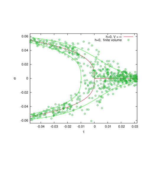
Figure 1: Scatter plot in the temperature-magnetization plane.

For a clearer explanation of our main assumption, let us consider a finite-volume ferromagnet as an example. One measures its magnetization $\sigma$ and temperature $\tau$ and marks each measurement by the respective point in the $\tau-\sigma$ plane (see green circles in Fig.1). However, in the infinite-volume limit, the distribution of such points shrinks to the red line corresponding to the critical behavior of the magnetization. Let us now consider some quantity $Q$ having a strong correlation with the magnetization (so that its temperature dependence is determined mainly by the magnetization) and then shift each point in the $\tau-\sigma-Q$ space along the abscissa $(\tau)$ axis so that its projection on the $\tau-\sigma$ plane gets into the red line. This results in only a little change of $Q$ because the magnetization remains unchanged. Now one is tempted to consider that the shifted (improved) data points make it possible to estimate $Q(\tau)$ in the infinite-volume limit using the data obtained in a relatively small volume. The additional information needed for such an estimate is provided by the knowledge of the infinite-volume behavior of the magnetization and the correlation between $Q$ and $\sigma$.

Since ${\cal P}$ and $-{\cal P}$ give the same temperature, the positive Polyakov-loop sector and the negative Polyakov loop sector should be treated separately - the more so the gluon propagators behave differently in different center sectors Silva:2016onh .

However, here we restrict our attention to the positive Polyakov-loop sector.

IV Decrease of finite-volume effects

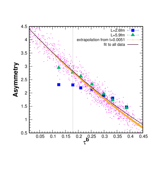
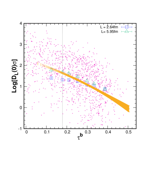
Figure 2: The results for the improvement procedure (yellow strips) are compared with the conventional averages obtained on the lattices of indicated sizes: squares are the small-size lattices and triangles — large-size lattices. Note that the extrapolation is performed using the data for smaller lattices. Vertical lines indicate the temperature from which the extrapolation was performed.

We rearrange the data obtained on a particular lattice (say, on that with $t=0.0051$ and $L=2.6fm$) using our improvement procedure in order to obtain the scatter plot in the asymmetry-temperature plane shown on the left panel of Fig.2. Then we perform regression analysis and employ the bootstrap technique in order to find the dependence of the average value of the asymmetry as the function of the temperature. The respective confidence corridor is shown by yellow strip.

Thus we perform extrapolation from a particular value of the temperature used in simulations to the range of temperature fluctuations associated with the Polyakov-loop fluctuations in the lattice volume under consideration. It is seen in Fig.2 that, in the critical domain, the range of temperature fluctuations is rather wide.

It is clearly seen that, at sufficiently small $\tau$ ($\tau\lesssim 0.02$), the improved data and, therefore, the improved average of the asymmetry is shifted to the values associated with substantially greater volumes. The significant deviation of the infinite-volume values of the asymmetry at $\tau\gtrsim 0.02$ can be explained by increasing role of the terms omitted in the approximate formula (11).

A similar procedure was performed with the data for the zero-momentum longitudinal propagator. We study the quantity ${\cal D}(\tau)=ln\Big{[}D_{L}(0)\sigma\Big{]}$ because the scatter in the data for $D_{L}(0)$ itself is so wide that it hinders statistical analysis (the width of the distribution in $D_{L}(0)$ depends severely on the temperature).

The results are shown on the right panel of Fig.2, we see the regularity similar to the case of the asymmetry. However, the difference between the asymmetry and the propagator is that the fraction of variance unexplained is much greater in the latter case.

In the case of asymmetry we also show the regression curve obtained from the regression with the bootstrap procedure for the combined data set (the data simulated at different lattices are mixed together). Justification of this operation is discussed below.

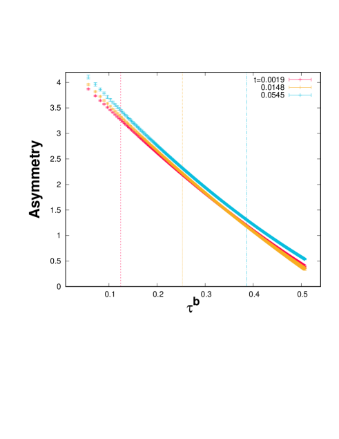
Figure 3: Confidence corridors for the extrapolations of the asymmetry from the data sets corresponding to the vertical dotted lines.

The confidence corridors for $f_{1}(t;\tau,V)$ (see formula (13) for a definition) at $t=0.0019$, $t=0.0148$ and $t=0.0545$ and $V=(2.6$ fm$)^{3}$ are shown in Fig.3. It is seen that the corridors for $t=0.0019$ and $t=0.0148$ are close to coincidence, whereas the corridor obtained for the $t=0.0545$ data deviates from the others. The confidence corridors for the other values of $t$ are not shown because it is difficult to present them in a common plot. However, our analysis reveals that the confidence corridors of the asymmetry values are substantially overlap for $t<0.02$ and begin to diverge from each other at greater values of $t$. Nevertheless, the divergence between the average asymmetries $\displaystyle|f_{t_{1},V}(\tau)-f_{t_{2},V}(\tau)|$ is more than order of magnitude smaller than the difference $\displaystyle|f_{t_{1},V}(t_{1})-f_{t_{1},V}(t_{2})|$ even in the worst case:

$$|f_{t_{1},V}(\tau)-f_{t_{2},V}(\tau)|<\!\!\!<|f_{t_{1},V}(t_{1})-f_{t_{1},V}(t_{2})|$$ (15)

$\forall\tau$ and $\forall t_{1},t_{2}$ under study. The latter quantity is related to the variation of the asymmetry owing to its temperature dependence through the Polyakov loop, the former — to its explicit temperature dependence. The data on $f_{t=0.0051,V}(\tau)$ are presented in the last column of Table 2.

Thus we conclude that the description of the temperature dependence of the asymmetry at the given volume in terms of its dependence on the Polyakov loop is reliable.

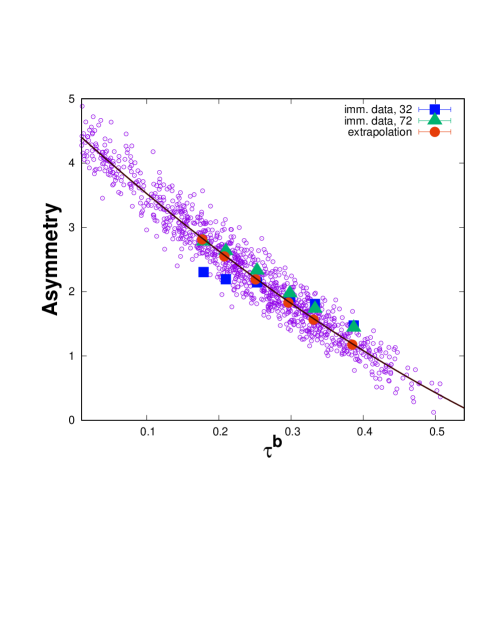
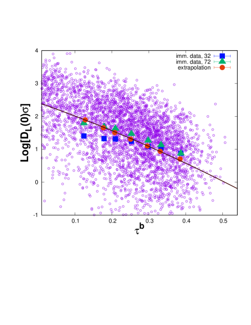
Figure 4: Asymmetry ${\cal A}(\tau)$ (left panel) and the logarithm of the zero-momentum longitudinal propagator ${\cal D}(\tau)$ (right panel) extrapolated from the temperature $t=-0.0013$ at $L=2.6$ fm are compared with the respective averages of the type (12): squares $L=2.6$ fm and triangles $L=6.0$ fm.

V An example of extrapolation from subcritical to supercritical temperatures

From the very beginning it should be emphasized that we rely on the knowledge of the critical behavior of the Polyakov loop, and work in a finite volume where temperature can fluctuate through the range under study. Therefore, such extrapolation is not forbidden by basic principles of theory.

We perform transformation of the data obtained on the lattice at $t=-0.0013$ and $L=2.6$ fm as follows:

$$(t,{\cal P},{\cal A},{\cal D})\to(\mathbf{p}_{V}^{-1}({\cal P}),{\cal P},{\cal A},{\cal D})\;.$$ (16)

and arrive at the scatter plot shown in Fig.4. The average values of the type (13) shown by solid curves are obtained by regression analysis with the use of the bootstrap technique (bootstrap errors within orange circles are not seen). It is demonstrated that the values extrapolated from the data for a small lattice size tend to approach the infinite-volume limit at $\tau<0.02$, deviations from this trend at larger values of $\tau$ can be explained by the need to take into account non-leading contributions in formula (11).

VI Conclusions

We have studied the temperature dependence of the chromoelectric-chromomagnetic asymmetry and the zero-momentum longitudinal gluon propagator at two different lattice sizes (2.6 fm and 6.0 fm) taking into account their correlation with the Polyakov loop.

Our estimates are approximate, however, they give clear evidence for the following:

• Finite-volume effects can be significantly decreased by performing data transformation (or improvement of the data) (16).

• The temperature dependence of the asymmetry ${\cal A}$ and the logarithm ${\cal D}$ of the dimensionless zero-momentum gluon propagator at the reduced temperature $\tau<0$.

• The data on the quantities under study at the reduced temperature $\tau<0$ involve information on their behavior at $\tau>0$. The extrapolation of the data related to a finite volume is possible through the range of temperature fluctuations.

• Correlations of fluctuating quantities and their consequences deserve more detailed studies with regard for finite-size scaling and corrections to the asymptotic critical behavior.

- (1) V. G. Bornyakov, V. V. Bryzgalov, V. K. Mitrjushkin and R. N. Rogalyov, Int. J. Mod. Phys. A 33 (2018) no.26, 1850151 doi:10.1142/S0217751X18501518 [arXiv:1801.02584 [hep-lat]].
- (2) V. G. Bornyakov, V. A. Goy, V. K. Mitrjushkin and R. N. Rogalyov, Phys. Rev. D 104 (2021) no.7, 074508 doi:10.1103/PhysRevD.104.074508 [arXiv:2101.03605 [hep-lat]].
- (3) M. N. Chernodub and E. M. Ilgenfritz, Phys. Rev. D 78 (2008), 034036 doi:10.1103/PhysRevD.78.034036 [arXiv:0805.3714 [hep-lat]].
- (4) V. G. Bornyakov, V. K. Mitrjushkin and R. N. Rogalyov, Phys. Rev. D 100 (2019) no.9, 094505 doi:10.1103/PhysRevD.100.094505 [arXiv:1609.05145 [hep-lat]].
- (5) B. Svetitsky and L. G. Yaffe, Nucl. Phys. B 210 (1982), 423-447 doi:10.1016/0550-3213(82)90172-9
- (6) F. Kos, D. Poland, D. Simmons-Duffin and A. Vichi, JHEP 08 (2016), 036 doi:10.1007/JHEP08(2016)036 [arXiv:1603.04436 [hep-th]].
- (7) J. Engels and T. Scheideler, Nucl. Phys. B 539 (1999), 557-576 doi:10.1016/S0550-3213(98)00781-0 [arXiv:hep-lat/9808057 [hep-lat]].
- (8) P.J. Silva and O. Oliveira, Phys. Rev. D 93 (2016), 114509; doi:10.1103/PhysRevD.93.114509”, arXiv:1601.01594 [hep-lat]