Pair Production in time-dependent Electric field at Finite times

I Introduction

A strong classical electromagnetic background can lead to vacuum instability and produce particle-antiparticle pairs. This process of particle creation from the quantum vacuum was first studied in 1951 by Schwinger under a constant electric field, and this phenomenon is known as the Schwinger effect PhysRev.82.664 .This particle creation paradigm has crucial importance for nonequilibrium processes in heavy-ion collisions24 ; 25 ; 26 as well as astrophysical phenomena27 and the search for nonlinear and nonperturbative effects in ultraintense laser systems12 ; 13 ; 14 .
Particle production is the process of evolving a quantum system from an initial equilibrium configuration to a new final equilibrium configuration via an intermediate non-equilibrium evolution caused by a strong field background. Such strong field QED pair production process has been investigated using scattering calculations Harvey:2009ry , exact solutions Dunne:1998ni , semi-classical techniques Kim:2000un ; DiPiazza:2004lsj , Monte Carlo simulations Gies:2005bz and quantum kinetic equations Alkofer:2001ik ; Blaschke:2005hs Quantitative description of particle production at all times in time-dependent electromagnetic field is not possible due to the absence of unique separation into positive and negative energy states at intermediate times and these positive and negative states are well-defined only at asymptotically early and late times where the field vanishes. A common approach is to define particle numbers in terms of an adiabatic basis using Bogoliubov transformation 2 ; 3 ; 4 ; 5 . In the adiabatic basis, we examine the problem of pair production in a time-varying spatially uniform Sauter electric field which has been studied by various authors 6 ; 44 . who calculated the number of particles created at the asymptotic time but the problem of particle production at the finite time is not studied for Sauter-Pulse electric field. We looking for the evolution of the quantum system at some initial time $t_{0}$ in the vacuum state but now what will be the properties of the quantum system at finite time $t$ ? What happens to the system properties at that non-asymptotic time? By finding the exact analytic solution of the mode function, which allows us to study the behaviour of the quantum vacuum during pair production at any instant of time for time-dependent Sauter pulsed electric fields in spinor quantum electrodynamics (QED). We use natural units and set $\hslash=c=m=1$ and express all variables in terms of the electron mass unit.

II Theory

Consider the creation of the electron-positron pair from vacuum by a linearly polarized time-dependent spatially uniform electric field along the $z$-axis which is characterized by the four-vector potential $A_{\mu}(t)=(0,0,0,A(t))$ with $E(t)=-\dot{A}(t).$ In our calculations, we choose the Sauter field in the direction of $z-$axis, which is given by

$$E(t)=-\dot{A}(t)=E_{0}sech^{2}(t/\tau)$$ (1)

and corresponding vector-potential

$$A(t)=-E_{0}\tau tanh(t/\tau).$$ (2)

where $E_{0}$ amplitude of the electric field and $\tau$ pulse duration of the electric field. The one-particle momentum distribution function $f(\textbf{p},t)$ is an important quantity in the description of the particle production process in the time-dependent electric field. As it was demonstrated in 41 ; 42 , f(p,t) can be written in terms of the mode solution as

$$f(\textbf{p},t)=\frac{{(\omega+\Pi)|\dot{\Psi}^{(\pm)}\pm i\omega\Psi^{(\pm)}|^{2}}}{2\omega}$$ (3)

where the mode equation 40 ; 43

$$\ddot{\Psi}^{(\pm)}+[\omega^{2}(t)\pm ie\dot{A}(t)]\Psi^{(\pm)}=0$$ (4)

with

$$\omega(t)^{2}=\Pi^{2}+\epsilon_{\perp}^{2},\quad\Pi=p_{z}+eA(t),\quad\epsilon_{\perp}^{2}=\textbf{p}_{\perp}^{2}+m^{2}.$$ (5)

For Sauter-Field, we are able to exactly solve the mode equation 4, which becomes the hyper-geometric differential equation and its solution is given in terms of hypergeometric functions. Using this solution, we calculate the one-particle distribution function in terms of hypergeometric functions. The time evolution of the particle distribution function $f(\textbf{p},t)$ in momentum space is studied for $E_{0}=0.2$ and $\tau=10.$

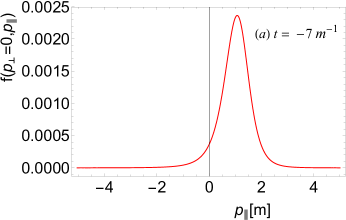
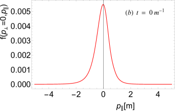
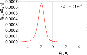
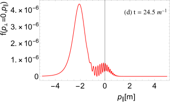
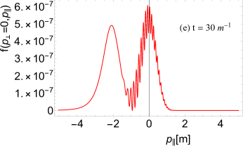
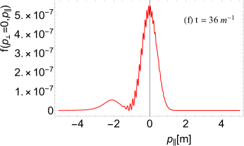
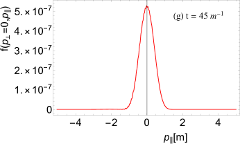
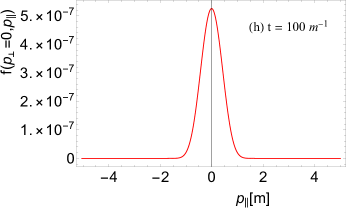
Figure 1: Time evolution of quasi-particle distribution function in the longitudinal momentum space $f(p_{\parallel},t)$ at different times. The transverse momentum is considered to zero, and all the units are taken in the electron mass units.The field parameters are $E_{0}=0.2E_{c}$ and $\tau=10.$

III Result

In this section, we discuss about both the longitudinal and transverse momentum spectrum of the created particle using the solution of the mode equation in 3 for $E_{0}=0.2$ and $\tau=10$.

III.1 Longitudinal momentum spectrum

In Figure 1, we show how the particle-creation proceeds. The produced electron is accelerated to the negative z-direction by the electric field. At early times (QEPP region 46 ) when electric field$E(t)$ is increasing, momentum distribution shows the smooth Gaussian-like structure and after reaching a maximum value at time $t=0$ electric field starts decaying, and we see the peak of the momentum distribution function is shifted as shown in figure 1(a),(b),(c). As time progresses, the distribution function tends to be peaked around the zero value of the longitudinal momentum as seen in figure 1(d). In this process, it shows a complex behavior of splitting and manifests oscillation arising at $t=3\tau$ (near REPP region ) where the electric field nearly vanished see figure 1(e),(f). These complex behavior disappear at the asymptotic time ( $t=10\tau$), and we see a smooth Gaussian-like structure 1(h).

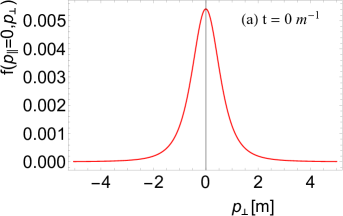
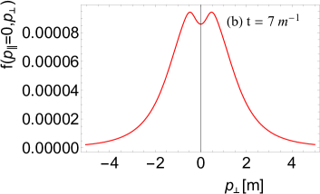
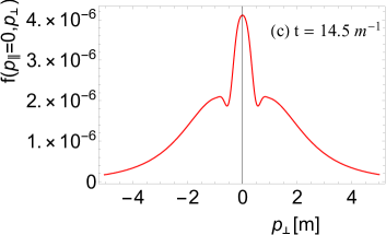
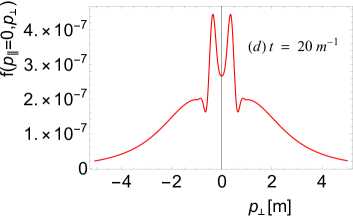
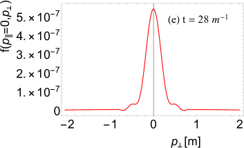
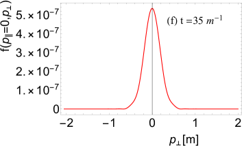
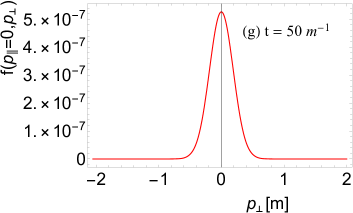
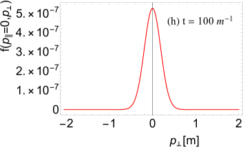
Figure 2: Time evolution of quasi-particle distribution function in the transverse momentum space $f(p_{\perp},t)$ at different times. The longitudinal momentum is considered to be zero, and all the units are taken in electron mass units.The field parameters are $E_{0}=0.2$ and $\tau=10.$

III.2 Transverse momentum spectrum

Time evolution of the transverse momentum spectrum of created quasi-particle pairs are depicted in the figure 2.The shape of the transverse momentum distribution is changed when the electric field is switched on. As we see in the figure 2(c),(d) at the transient stage the peak at $p_{\perp}=0$ splits into weakly pronounced peaks at $p_{\perp}\approx\pm 0.67m$ and $p_{\perp}\approx\pm 0.84m.$ At the asymptotic time (REPP stage 46 ), that splitting disappears and distribution function $f(p_{\perp})$ shows the smooth structure with a peak at zero transverse momentum as shown in figure 2(h).

IV Conclusion

We have analyzed the electron-positron pair creation from the vacuum by a time-like Sauter pulse electric field. We have seen that the particle Longitudinal momentum distributions exhibit the oscillating structure at a finite time where the electric field is nearly zero and this oscillating structure can be understood in the Dynamical Tunneling picture45 . Dynamical tunneling can be understood as the process that develops in time inter-band dynamics in momentum representation for particles. There are different possibilities of particle tunneling through different channels in momentum space( or momentum states). As time progresses, different possibilities can occur: (a) particle can tunnel at time $t$ with $p_{\parallel}^{\prime}-$value of momentum. (b)At early stage, particle with a lower momentum value ($p_{\parallel}<p_{\parallel}^{\prime}$) can tunnel and then be accelerated to momentum $p_{\parallel}^{\prime}$, (c)Particle with a higher momentum value ($p_{\parallel}>p_{\parallel}^{\prime}$) can tunnel at time, $t_{1}$, and is then decelerated to get that momentum $p_{\parallel}^{\prime}$ value. Finally, when the individual probability amplitudes of this process are added together, they result in quantum interference at time $t$.  At the asymptotic time, those processes do not share the same phase information and become random due to averaging over particle paths that do not show quantum interference effects, which leads to a smooth distribution function. However, multiphoton absorption is not seen for the value of the Keldysh parameter $\gamma<1,$ but it is believed to give a smaller contribution in comparison to what we get from tunneling. Since, in our calculation, it is not much less than one ($\gamma=0.5$). As a result, another process of particle creation with momentum $p_{\parallel}$, namely the multiphoton process, cannot be ruled out. These are possibilities, and extensive quantitative analyses of these processes are in progressDEEPAK:2023 . The transverse momentum distribution shows only the splitting of smooth structure and the absence of quantum interference, which is an obvious interference effect that occurs only in the direction of the electric field.
A more detailed investigation of the momentum distribution of created particles at the finite time is currently underway DEEPAK:2023 .

V Acknowledgments

DEEPAK gratefully acknowledge the financial support from Homi Bhabha National Institute (HBNI) for carrying out this research work. Deepak also thanks the organizers of the QED Laser Plasmas International Workshop 2022, Dresden for the possibility to present our work.

References

- (1) J. Schwinger, On gauge invariance and vacuum polarization, Phys. Rev. 82, 664 (1951).
- (2) F. Gelis and R. Venugopalan, Particle production in field theories coupled to strong external sources, I: Formalism and main results, Nucl. Phys. A776, 135 (2006).
- (3) D. Kharzeev and K. Tuchin, Multi-particle production and thermalization in high-energy QCD, Phys. Rev. C 75, 044903 (2007).
- (4) F. Gelis, E. Iancu, J. Jalilian-Marian, and R. Venugopalan, The color glass condensate, Annu. Rev. Nucl. Part. Sci. 60, 463 (2010).
- (5) R. Ruffini, G. Vereshchagin, and S. Xue, Electron-positron pairs in physics and astrophysics: From heavy nuclei to black holes, J. Phys. Rep. 487, 1 (2010).
- (6) M. Marklund and P. Shukla, Nonlinear collective effects in photon photon and photon plasma interactions, Rev. Mod. Phys. 78, 591 (2006).
- (7) A. Di Piazza, C. Muller, K. Z. Hatsagortsyan, and C. H. Keitel, Extremely high-intensity laser interactions with fundamental quantum systems, Rev. Mod. Phys. 84, 1177 (2012).
- (8) G. Mourou, T. Tajima, and S. Bulanov, Optics in the relativistic regime, Rev. Mod. Phys. 78, 309 (2006).
- (9) C. Harvey, T. Heinzl and A. Ilderton, “Signatures of High-Intensity Compton Scattering,” Phys. Rev. A 79 (2009), 063407
- (10) G. V. Dunne and T. Hall, “On the QED effective action in time dependent electric backgrounds,” Phys. Rev. D 58 (1998), 105022
- (11) S. P. Kim and D. N. Page, “Schwinger pair production via instantons in a strong electric field,” Phys. Rev. D 65 (2002), 105002
- (12) A. Di Piazza, “Pair production at the focus of two equal and oppositely directed laser beams: The effect of the pulse shape,” Phys. Rev. D 70 (2004), 053013
- (13) H. Gies and K. Klingmuller, “Pair production in inhomogeneous fields,” Phys. Rev. D 72 (2005), 065001
- (14) R. Alkofer, M. B. Hecht, C. D. Roberts, S. M. Schmidt and D. V. Vinnik, “Pair creation and an x-ray free electron laser,” Phys. Rev. Lett. 87 (2001), 193902 doi:10.1103/PhysRevLett.87.193902 [arXiv:nucl-th/0108046 [nucl-th]].
- (15) D. B. Blaschke, A. V. Prozorkevich, C. D. Roberts, S. M. Schmidt and S. A. Smolyansky, ‘Pair production and optical lasers,” Phys. Rev. Lett. 96 (2006), 140402 doi:10.1103/PhysRevLett.96.140402 [arXiv:nucl-th/0511085 [nucl-th]].
- (16) E. Brezin and C. Itzykson, Pair production in vacuum by an alternating field, Phys. Rev. D 2, 1191 (1970)
- (17) V. S. Popov, Pair production in a variable external field (quasiclassical approximation), Sov. Phys. JETP 34, 709 (1972); Pair production in a variable and homogeneous electric fields as an oscillator problem, Sov. Phys. JETP 35, 659 (1972).
- (18) D. Gitman and S. Gavrilov, Quantum processes in a strong electromagnetic field. Creating pairs, Izv. Vuz. Fiz. 1, 94 (1977).
- (19) F. Gelis and N. Tanji, Schwinger mechanism revisited, Prog. Part. Nucl. Phys. 87, 1 (2016).
- (20) S. P. Gavrilov and D. M. Gitman, Vacuum instability in external fields, Phys. Rev. D 53, 7162 (1996).
- (21) A. B. Balantekin, J. E. Seger and S. H. Fricke, Dynamical effects in pair production by electric fields, Int. J. Mod. Phys. A 6 (1991) 695.
- (22) Y. Kluger, J. M. Eisenberg, B. Svetitsky, F. Cooper and E. Mottola, “Pair production in a strong electric field”, Phys. Rev. Lett. 67, 2427 (1991).
- (23) Y. Kluger, J. M. Eisenberg, B. Svetitsky, F. Cooper and E. Mottola, “Fermion pair production in a strong electric field”, Phys. Rev. D 45, 4659 (1992).
- (24) A. M. Fedotov, E. G. Gelfer, K. Yu Korolev and S. A. Smolyansky, Kinetic equation approach to pair production by a time-dependent electric field, Phys. Rev. D, 83, 025011 (2011).
- (25) S. P. Kim and C. Schubert, “Nonadiabatic quantum Vlasov equation for Schwinger pair production,” Phys. Rev. D 84, 125028 (2011).
- (26) L.V. Keldysh, Dynamic Tunneling. Her. Russ. Acad. Sci. 86, 413–425 (2016).
- (27) D.B. Blaschke,S.A. Smolyansky, A.Panferov,L.Juchnowski,Particle production in strong time-dependent fields. In Proceedings of the Quantum Field Theory at the Limits: From Strong Fields to Heavy Quarks (HQ 2016), Dubna, Russia, 18–30 July 2016.
- (28) Deepak and Manoranjan P. Singh, Pair Production in time-dependent Electric field at Finite times, in preparation.