Sparsity based morphological identification of heartbeats

Abstract

Automation of heartbeat identification. Sparse representations. Greedy pursuit strategies. Computerised ECG interpretation.

1 Introduction

Cardiovascular diseases (CDVs) are a group of disorders of the heart and blood vessels, including coronary heart disease, cardiovascular disease, rheumatic heart disease and other conditions. These diseases are the leading cause of global death. The World Health Organisation (WHO) estimates that 32% of all deaths worldwide are caused by CDVs. In addition to preventing CDVs by maintaining a healthy lifestyle, early detection can curb mortality rates for heart disease patients and also for people with increased risk of this condition.

An electrocardiogram (ECG) is a safe and non-invasive procedure that detects cardiac abnormalities by measuring the electrical activity generated by the heart as it contracts. Sensors attached to the skin are used to detect the electrical signals produced by the heart each time it beats. These signals are analysed by a specialist to assess if they are unusual. Computerised ECG analysis plays a critical role in clinical ECG workflow. It is predicted that in the future full automated analysis of ECG may become more reliable than human analysis.

Automation of ECG interpretation has been successfully addressed by Artificial Intelligence (AI) methods which fall within the end-to-end deep learning framework [1, 2, 3, 4]. However, due to the over-parameterised black-box nature of this framework [5] it is difficult to understand how deep models make decisions. Besides, interpretation using Deep Neural Networks (DNN) has been shown to be susceptible to adversarial attacks [6, 7]. Automatic classification of heartbeats has also been addressed by different techniques of machine learning which rely on the ability to extract distinctive features of the beats in each class. Reviews and summaries of these techniques can be found in [8, 9, 10, 11].

In this work we present an alternative viewpoint for the specific task of morphological identification of heartbeats. We base the proposed method on the ability to model the morphology of a heartbeat as superposition of elementary components. We work under the assumption that there exits a set of elementary component which is better suited for representing heartbeats of certain morphology than others. Inspired by a previous work on face recognition [12], we consider that the sets of elementary components are redundant. However, we differ from [12] in the methodology and also in that here the redundant sets are to be learned from data. The common ground between the approaches is that both base the identification criterion on the concept of sparsity.

In the signal processing field, a signal approximation is said to be sparse if it belongs to a subspace of much smaller dimensionality than that of the space were the signal comes from. The search for the approximation subspace is carried out using a redundant set, called a ‘dictionary’. Only a few elements of the dictionary, called ‘atoms’, are finally used for constructing the signal approximation, called ‘atomic decomposition’. Sparse approximation of heartbeats is applied in [13] for classification using Gabor dictionaries. The particular Gabor’s atoms involved in the representation of the beats, as well as the coefficients in the atomic decomposition, are taken as features to feed machine learning classifiers. Contrarily, our proposal relies on the possibility of learning dictionaries, which play themselves a central role in the decision making process. To the best of our knowledge this setup has not been considered before. We focus on the layout of the approach and test it for binary classification.

The paper is organised as follows. Sec. 2 discuses the greedy algorithms to be considered, as well as the method for learning the dictionaries. The sparsity metrics supporting the discrimination criteria are also introduced in this section. The numerical tests illustrating the approach are placed in Sec. 3. The conclusions are drawn in Sec. 4.

2 Signal representation using dictionaries

We start this section by introducing some basic notation. Throughout the paper $\mathbb{R}$ represents the set of real numbers, and $\mathbb{N}$ and $\mathbb{Z}$ the sets of natural and integer numbers respectively. Boldface lower case letters indicate Euclidean vectors and boldface capital letters indicate matrices. The corresponding components are indicated using standard mathematical fonts e.g., $\mathbf{d}\in\mathbb{R}^{N}$ is a vector of components $d(i)\in\mathbb{R},\,i=1,\ldots,N$ and $\mathbf{G}\in\mathbb{R}^{N\times M}$ is a matrix of components $G(i,j),\ i=1,\ldots,N,\,j=1,\ldots,M$. The Euclidean inner product $\left\langle\cdot,\cdot\right\rangle$ between vectors in $\mathbb{R}^{N}$ is defined as

$$\left\langle\mathbf{d},\mathbf{g}\right\rangle=\sum_{i=1}^{N}d(i)g(i).$$

This definition induces the 2-norm $\|\mathbf{g}\|=\sqrt{\left\langle\mathbf{g},\mathbf{g}\right\rangle}$. The 1-norm of a vector $\mathbf{c}\in\mathbb{R}^{N}$, is indicated as $\|\mathbf{c}\|_{1}$ and calculated as $\|\mathbf{c}\|_{1}=\sum_{n=1}^{N}|c(n)|$.

The inner product between matrices in $\mathbb{R}^{N\times M}$ is the Frobenius inner product, which is defined as

$$\left\langle\mathbf{F},\mathbf{G}\right\rangle_{F}=\sum_{i=1}^{N}\sum_{j=1}^{M}F(i,j)G(i,j).$$

This definition induces the Frobenius norm $\|\mathbf{G}\|_{F}=\sqrt{\left\langle\mathbf{G},\mathbf{G}\right\rangle_{F}}.$ The transpose of a matrix $\mathbf{G}$ is indicated as $\mathbf{G}^{\top}$.

Given a signal $\mathbf{f}$ as a vector in $\mathbb{R}^{N}$, the $K$-term atomic decomposition for its approximation is of the form

$$\mathbf{f}^{K}=\sum_{n=1}^{K}c(n)\mathbf{d}_{\ell_{n}},$$ (1)

where the elements $\mathbf{d}_{\ell_{n}}$, called atoms, are chosen from a redundant set $\mathcal{D}=\{\mathbf{d}_{n},\in\mathbb{R}^{N},\|\mathbf{d}_{n}\|=1\}_{n=1}^{M}$, called dictionary. The set of all linear combination of elements in $\mathcal{D}$ is denoted as ${\mbox{\rm{span}}}\{\mathcal{D}\}$. The problem of how to select from $\mathcal{D}$ the $K$ elements $\mathbf{d}_{\ell_{n}},\,n=1\ldots,K$ such that $\|\mathbf{f}^{K}-\mathbf{f}\|$ is minimal is intractable (there are $\frac{N!}{(N-K)!K!}$ possibilities). In practical applications the problem is addressed by ‘tractable’ methods. For the most part these methods are realised by

• Expressing $\mathbf{f}^{K}=\sum_{n=1}^{M}c(n)\mathbf{d}_{n}$ using only $K$-nonzero coefficients minimising the 1-norm $\|\mathbf{c}\|_{1}=\sum_{n=1}^{M}|c(n)|$ [14].

• Using a greedy pursuit strategy for stepwise selection of the $K$ elements $\mathbf{d}_{\ell_{n}},\,n=1,\ldots,K$, for producing the approximation (1).

We restrict consideration to greedy pursuit algorithms, because for the application we are considering these types of methods are effective and faster that those based on minimisation of the 1-norm.

2.1 Pursuit Strategies

In the context of signal processing the simplest pursuit strategy is known under the name of Matching Pursuit (MP)[15]. Depending on their implementation and context of application variations of the MP approach can also be found under different names. We discuss here a refinement of MP known as Orthogonal Matching Pursuit (OMP) [16] as well as the stepped wise optimised version termed Optimised Orthogonal Matching Pursuit (OOMP) [17].

2.1.1 From MP to OMP

The MP algorithm evolves by successive approximations as follows: Setting $k=0$ and starting with an initial approximation $\mathbf{f}^{0}=0$ and residual $\mathbf{r}^{0}=\mathbf{f}$, the algorithm progresses by sub-decomposing the $k$-th order residual in the form

$$\mathbf{r}^{k}=\left\langle\mathbf{d}_{\ell_{k+1}},\mathbf{r}^{k}\right\rangle\mathbf{d}_{\ell_{k+1}}+\mathbf{r}^{k+1},$$ (2)

where $\mathbf{d}_{\ell_{k+1}}$ is the atom corresponding to the index selected as

$$\ell_{k+1}=\operatorname*{arg\,max}_{\begin{subarray}{c}n=1,\ldots,M\end{subarray}}|\left\langle\mathbf{d}_{n},\mathbf{r}^{k}\right\rangle|.$$ (3)

This atom is used to update the approximation $\mathbf{f}^{k}$ as

$$\mathbf{f}^{k+1}=\mathbf{f}^{k}+\left\langle\mathbf{d}_{\ell_{k+1}},\mathbf{r}^{k}\right\rangle\mathbf{d}_{\ell_{k+1}}.$$ (4)

From (2) it follows that $\|\mathbf{r}^{k+1}\|\leq\|\mathbf{r}^{k}\|$, since

$$\|\mathbf{r}^{k}\|^{2}=|\left\langle\mathbf{d}_{\ell_{k+1}},\mathbf{r}^{k}\right\rangle|^{2}+\|\mathbf{r}^{k+1}\|^{2}.$$ (5)

It is easy to prove that in the limit $k\rightarrow\infty$, the sequence $\mathbf{f}^{k}$ given in (4) converges to $\mathbf{f}$, if $\mathbf{f}\in V_{M}={\mbox{\rm{span}}}\{\mathcal{D}\}$, or to $\hat{P}_{V_{M}}\mathbf{f}$ the orthogonal projection of $\mathbf{f}$ onto $V_{M}$, if $\mathbf{f}\notin V_{M}$ (a pedagogical proof can be found on [18]). However, the method is not stepwise optimal because it does not yield an orthogonal projection at each step. Accordingly, the algorithm may select linearly dependent atoms, which is the main drawback of MP when applied with highly coherent dictionaries. A refinement to MP, which does yield an orthogonal projection approximation at each step is called OMP [16]. The method selects the atoms as in (3) but at each iteration produces a decomposition of the signal as given by:

$$\mathbf{f}^{k}=\sum_{n=1}^{k}c^{k}(n)\mathbf{d}_{\ell_{n}}+\tilde{\mathbf{r}}^{k},$$ (6)

where the coefficients $c^{k}(n)$ are computed in such a way that it is true that

$$\sum_{n=1}^{k}c^{k}(n)\mathbf{d}_{\ell_{n}}=\hat{P}_{\mathtt{V}_{k}}\mathbf{f},\quad{\text{with}}\quad V_{k}={\mbox{\rm{span}}}\{\mathbf{d}_{\ell_{n}}\}_{n=1}^{k}.$$

The superscript of $c^{k}(n)$ in (6) indicates the dependence of these quantities on the iteration step $k$. Thus, in addition to selecting linearly independent atoms, OMP yields the unique element $\mathbf{f}^{k}\in V_{k}$ minimising $\|\mathbf{f}^{k}-\mathbf{f}\|$. As discussed next, a further refinement to OMP, called OOMP [17], selects also the atoms in order to minimise in a stepwise manner the norm of the residual error.

2.1.2 The OOMP method

The OOMP approach iterates as follows. The algorithm is initialised by setting: $\mathbf{r}^{0}=\mathbf{f}$, $\mathbf{f}^{0}=0$, $\Gamma=\emptyset$ and $k=0$. The first atom is selected as the one corresponding to the index $\ell_{1}$ such that

$$\ell_{1}=\operatorname*{\,max}_{n=1,\ldots,M}\left|\left\langle\mathbf{d}_{n},\mathbf{r}^{0}\right\rangle\right|^{2}.$$ (7)

This first atom is used to assign $\mathbf{w}_{1}=\mathbf{d}_{\ell_{1}}=\boldsymbol{\beta}_{1}$, calculate $\mathbf{r}^{1}=\mathbf{f}-\mathbf{d}_{\ell_{1}}\left\langle\mathbf{d}_{\ell_{1}},\mathbf{f}\right\rangle$, and iterate as prescribed below.

• Upgrade the set $\Gamma\leftarrow\Gamma\cup\ell_{k+1}$, increase $k\leftarrow k+1$, and select the index of a new atom for the approximation as

  $$\ell_{k+1}=\operatorname*{\,max}_{\begin{subarray}{c}n=1,\ldots,M\\ n\notin\Gamma\end{subarray}}\frac{|\left\langle\mathbf{d}_{n},\mathbf{r}^{k}\right\rangle|^{2}}{1-\sum_{i=1}^{k}|\left\langle\mathbf{d}_{n},\tilde{\mathbf{w}}_{i}\right\rangle|^{2}},\quad\text{with}\quad\tilde{\mathbf{w}}_{i}=\frac{\mathbf{w}_{i}}{\|\mathbf{w}_{i}\|_{2}}.$$ (8)

• Compute the corresponding new vector $\mathbf{w}_{k+1}$ as

  $$\begin{split}\mathbf{w}_{k+1}=\mathbf{d}_{\ell_{k+1}}-\sum_{n=1}^{k}\frac{\mathbf{w}_{n}}{\|\mathbf{w}_{n}\|^{2}_{2}}\left\langle\mathbf{w}_{n},\mathbf{d}_{\ell_{k+1}}\right\rangle.\end{split}$$ (9)

  including, for numerical accuracy, the re-orthogonalisation step:

  $$\mathbf{w}_{k+1}\leftarrow\mathbf{w}_{k+1}-\sum_{n=1}^{k}\frac{\mathbf{w}_{n}}{\|\mathbf{w}_{n}\|_{2}^{2}}\left\langle\mathbf{w}_{n},\mathbf{w}_{k+1}\right\rangle.$$ (10)

• Upgrade vectors $\boldsymbol{\beta}_{n}^{k}$ as

  $$\boldsymbol{\beta}_{k+1}^{k+1}=\frac{\mathbf{w}_{k+1}}{\|\mathbf{w}_{k+1}\|^{2}},\quad\boldsymbol{\beta}_{n}^{k+1}=\boldsymbol{\beta}_{n}^{k}-\boldsymbol{\beta}_{k+1}^{k+1}\left\langle\mathbf{d}_{\ell_{k+1}},\boldsymbol{\beta}_{n}^{k}\right\rangle,\quad n=1,\ldots,k.$$ (11)

• Upgrade vector $\mathbf{r}^{k}$ as

  $$\mathbf{r}^{k+1} = \mathbf{r}^{k}-\left\langle\mathbf{w}_{k+1},\mathbf{f}\right\rangle\frac{\mathbf{w}_{k+1}}{\|\mathbf{w}_{k+1}\|^{2}}.$$ (12)

• If for a given $\rho$ value the condition $\|\mathbf{r}^{k+1}\|<\rho$ has been met stop the selection process. Otherwise repeat steps 1) - 5).

Calculate the coefficients in (1) as

$$\mathbf{c}=\left\langle\boldsymbol{\beta},\mathbf{f}\right\rangle.$$

Calculate the final approximation $\mathbf{f}^{k}$ as

$$\mathbf{f}^{k}=\mathbf{f}-\mathbf{r}^{k}.$$

Remark 1.

The difference between our implementations of OMP and OOMP is only that for OMP the denominator in (8) is eliminated. The selection is realised as in MP (c.f. (3)) which is not a stepwise optimal selection. Instead, (8) selects the atom $\mathbf{d}_{\ell_{k+1}}$ which, fixing the previously selected atoms $\mathbf{d}_{\ell_{i}},\,i=1,\ldots,k$, minimises the distance $\|\mathbf{f}^{k+1}-\mathbf{f}\|$. The proof can be found in [17].

2.2 Sparsity criterion for morphological feature extraction of heartbeats

A digital ECG signal is a sequence of heartbeats, each of which is characterised by a combination of three graphical deflections, known as QRS complex, and the so called P and T waves. An idealised illustration of these deflections are given in Fig. 1.

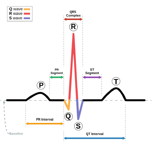
Figure 1: Public domain graph of the QRS complex and P and T waves representing a normal heartbeat.

However, as illustrated in Fig. 2, in real ECG records the shape of the beats in the same class may vary.

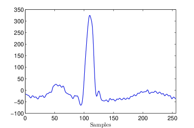
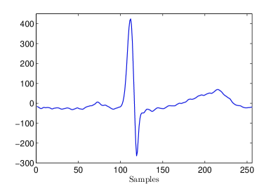
Figure 2: Two normal heartbeats from different ECG records

Approximation for morphological feature extraction of a heartbeat requires the segmentation of the QRS complex. In this work the segmentation is realised by taking a fixed number of samples to left and right of the location of the R-peak, to have beats of equal support, say $N_{q}$.

Assuming that one wishes to morphologically differentiate heartbeats of, say class $\mathtt{A}$, from heartbeats of class $\mathtt{B}$, and that a dictionary $\mathcal{D}_{\mathrm{a}}$, specially constructed to approximate a heartbeat of class $\mathtt{A}$, and a dictionary $\mathcal{D}_{\mathrm{b}}$, specially constructed to approximate a heartbeat of class $\mathtt{B}$, are given, we discuss next several possibilities of using sparsity as a distinguishability criterion.

In order to decide whether a heartbeat $\mathbf{f}\in\mathbb{R}^{N_{q}}$ belongs to class $\mathtt{A}$ or class $\mathtt{B}$ this beast is approximated, up to the same precision, using both dictionaries, i.e.

$$\mathbf{f}^{a}=\sum_{n=1}^{K_{a}}c^{a}(n)\mathbf{d}_{\ell_{n}^{a}},$$ (13)

where the atoms $\mathbf{d}_{\ell_{n}^{a}}$ are chosen from $\mathcal{D}_{\mathrm{a}}$ and

$$\mathbf{f}^{b}=\sum_{n=1}^{K_{b}}c^{b}(n)\mathbf{d}_{\ell_{n}^{b}},$$ (14)

where the atoms $\mathbf{d}_{\ell_{n}^{b}}$ are chosen from $\mathcal{D}_{\mathrm{b}}$.

Criterion I (a) and (b)

If $K_{a}<K_{b}$ the beat $\mathbf{f}_{q}$ is assigned to class $\mathtt{A}$.
If $K_{b}<K_{a}$ the beat $\mathbf{f}_{q}$ is assigned to class $\mathtt{B}$.
If $K_{a}=K_{b}$ the criterion does not make a decision.

In the event that $K_{a}=K_{b}$ a decision could still be made by recourse to a different metric.

(a) Smaller entropy criterion: Assigning $p^{a}(n)=\frac{|c^{a}(n)|}{\|\mathbf{c}^{a}\|_{1}}$ and $p^{b}(n)=\frac{|c^{b}(n)|}{\|\mathbf{c}^{b}\|_{1}}$ calculate the corresponding Shannon’s entropies

$$S^{a}=-\sum_{n=1}^{K_{a}}p^{a}(n)\ln(p^{a}(n)),$$

$$S^{b}=-\sum_{n=1}^{K_{b}}p^{b}(n)\ln(p^{b}(n)).$$

The entropy of, say $p^{a}(n),\,n=1,\ldots,K_{a}$, would be smaller if the components are fewer and the magnitude of some $p^{a}(n)$ much larger than others. In particular the minimum entropy value occurs if $p^{a}(n)=\frac{|c^{a}(n)|}{\|\mathbf{c}^{a}\|_{1}}=1$ for some $n$ and zero otherwise, in which case $S^{a}=0$. Accordingly, if $S_{a}<S_{b}$ the beat $\mathbf{f}$ might be assigned to class $\mathtt{A}$ and if $S_{b}<S_{a}$ the beat $\mathbf{f}$ might be assigned to class $\mathtt{B}$. Let us recall that the criterion of smaller entropy was introduced for basis selection in the context of wavelet packets [23].

(b) Smaller norm-1 criterion.
This criterion is in line with the basis pursuit approach [14] which adopts the minimisation of the norm-1 as a way of producing a tractable sparse solution from a given dictionary. Consequently, if $\|\mathbf{c}^{a}\|_{1}<\|\mathbf{c}^{b}\|_{1}$ the beat $\mathbf{f}$ is assigned to class $\mathtt{A}$ and if $\|\mathbf{c}^{b}\|_{1}<\|\mathbf{c}^{a}\|_{1}$ the beat $\mathbf{f}$ if be assigned to class $\mathtt{B}$.

Criterion II

Use always the smaller entropy criterion.

Criterion III

Use always the smaller norm-1 criterion.

2.3 Dictionary learning

So far we have assumed to know the dictionaries $\mathcal{D}_{\mathrm{a}}$ and $\mathcal{D}_{\mathrm{b}}$, best suited for each class of heartbeat. In this section we discuss how these dictionaries can be learnt from a data set of annotated heartbeats.

The adopted strategy to learn a dictionary, as a matrix $\mathbf{D}$, using the heartbeats placed in an array $\mathbf{F}\in\mathbb{R}^{N_{q}\times Q}$ proceed through a 2 step process.

Step 1

• Set $k=0$. Given an initial dictionary, as a matrix $\mathbf{D}^{k}\in\mathbb{R}^{N_{q}\times M}$, use a greedy algorithm to approximate each beat $\mathbf{f}_{q}\in\mathbb{R}^{N_{q}}$, for $q=1,\ldots,Q$, as in (13) or (14) and collect the vectors of coefficients $\mathbf{c}_{q}^{k}\in\mathbb{R}^{K_{q}}$.

• Place each vector $\mathbf{c}_{q}^{k}$ as a column of a matrix $\mathbf{C}^{k}\in\mathbb{R}^{M\times Q}$ having nonzero elements $C{({\ell_{n}^{q}},q)}^{k}={c_{q}(n)}^{k},\,n=1,\ldots,{K_{q}}^{k},\,q=1,\ldots,Q$ and set all the other elements equal to zero.

• Using matrix $\mathbf{C}^{k}$ and dictionary $\mathbf{D}^{k}$ calculate the approximation $\tilde{\mathbf{F}}$ of $\mathbf{F}$ as

  $$\tilde{\mathbf{F}}^{k}=\mathbf{D}^{k}\mathbf{C}^{k}$$

Step 2

• Using the approximation $\tilde{\mathbf{F}}^{k}$ find the updated dictionary $\mathbf{D}^{k+1}$ minimising $\|\tilde{\mathbf{F}}-\tilde{\mathbf{F}}^{k}\|_{F}^{2}$. Thus,

  $$\mathbf{D}^{k+1}=\operatorname*{arg\,min}_{\begin{subarray}{c}\mathbf{D}\end{subarray}}\|{\tilde{\mathbf{F}}}-{\mathbf{D}}\mathbf{C}^{k}\|_{F}^{2}={\tilde{\mathbf{F}}}{\mathbf{C}^{k}}^{\top}(\mathbf{C}^{k}{\mathbf{C}^{k}}^{\top})^{-1}.$$ (15)

• Given a maximum number of iterations, $\operatorname*{MaxIt}$ say, and a tolerance $\mathrm{tol}$ for the error norm, if $\|\mathbf{D}^{k+1}-\mathbf{D}^{k}\|_{F}<\mathrm{tol}$ or $k+1>\operatorname*{MaxIt}$ stop. Otherwise set $k\to k+1$ and repeat Steps 1 and 2.

Remark 2.

The dictionary updating equation (15) requires that matrix $\mathbf{C}^{k}{\mathbf{C}^{k}}^{\top}$ should have an inverse. This would not be true if some elements in the dictionary were not chosen in the previous step. In that case, the unselected atoms should be removed from the dictionary before implementing equation (15). In practice, as long as $Q$ is significantly larger than $M$ and the examples are independent, matrix $\mathbf{C}^{k}{\mathbf{C}^{k}}^{\top}$ has an inverse.

Remark 3.

The problems of determining matrix $\mathbf{C}^{k}$ at Step 1 and matrix $\mathbf{D}$ at Step 2 are convex problems with unique solution. However, the combined problem of determining matrix $\mathbf{C}^{k}$ and $\mathbf{D}$ is not jointly convex. Thus, the solution depends on the initial dictionary. As will be demonstrated by the simulations, this in not crucial within the context of the proposed approach.

3 Binary morphological differentiation of heartbeats

In this section we test the proposal by differentiating the classes ${\tt{N}}$ (Normal) and ${\tt{V}}$ (Ventricular Ectopic) in the MIT-BIH Arrhythmia data set [19, 20]. As per the recommendations given by the Advancement of Medical Instrumentation (AAMI) the MIT-BIH Arrhythmia database is projected into five classes. Within these classes the ${\tt{N}}$ beats considered here include: The normal beats N, the Left Bundle Branch Block Beats (LBB) and the Right Bundle Branch Block Beats (RBB). The ${\tt{V}}$ class comprises: the Premature Ventricular Contraction (PVC) and Ventricular Escape Beats (VEB). While the number of ${\tt{V}}$ beats is much less than the number of ${\tt{N}}$ beats, the former are still enough to learn the corresponding dictionary. The locations of the R-peaks are retrieved from the annotations provided with the dataset, using the Matlab software [21] available on [19]. The peaks are then segmented by taking $145$ samples to the right and 110 samples to the left of the R-peak location. Before learning the dictionary a quick check of the training set is realised, in order to find out if there are some peaks that would not qualify as ‘good’ examples. For this end we proceed as explained below.

Screening the data training sets

For automatic screening of a set the segmented beats of the same class are approximated, up to the same quality, using a greedy algorithm and a general wavelet dictionary. We illustrate the process by giving the details for screening the training set for the numerical Test I.

Wavelet dictionaries arise from translations, by a parameter $b=2^{-l},\,l\in\mathbb{N}$ of scaling prototypes [24, 25]

$$\phi_{j_{0},k,b}\left(x\right)=\phi\left(2^{j_{0}}x-bk\right),\quad k\in\mathbb{Z},$$ (16)

and wavelet prototypes at different scales

$$\psi_{j,k,b}\left(x\right)=\psi\left(2^{j}x-bk\right),\quad k\in\mathbb{Z},\quad j\geq j_{0}.$$ (17)

For screening of the training set we have used the 9$/$7 Cohen-Daubechies-Feauveau (cbf97) wavelet family with $b=0.25$, $j_{0}=2$ and $j=3,4,5,6$, which introduces a redundancy factor of 2.67. This dictionary was generated with the software described in [26] available on [27]. The scaling and wavelet prototypes for the cbf97 wavelet family are shown in Fig. 3.

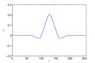
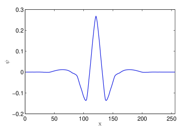
Figure 3: Graph of the scaling prototype $\phi(x)$ (left) and wavelet prototype $\psi(x)$ (right) for the cbf97 family.

The quality in the approximation of each beat is fixed using the ${\mathrm{prdn}}$ metric as defined by

$${\mathrm{prdn}}(q)=\frac{\|\mathbf{f}_{q}-\mathbf{f}_{q}^{k}\|}{\|\mathbf{f}_{q}-\overline{\mathbf{f}}_{q}\|}\times 100\%,\quad q=1,\ldots,Q,$$

where each $\mathbf{f}_{q}$ is a heartbeat, $\mathbf{f}_{q}^{k}$ its corresponding approximation by $k$ atoms, and $\overline{\mathbf{f}}_{q}$ the mean value of $\mathbf{f}_{q}$. The approximation of different beasts, up to the same ${\mathrm{prdn}}$, is achieved for different values of $k$. The left graph of Fig.4 shows the histograms of $k$ values obtained when approximating, up to ${\mathrm{prdn}}=9$, the ${\tt{N}}$ beats in the training set of the numerical Test I (c.f. Sec. 3.1).

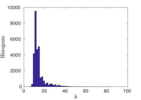
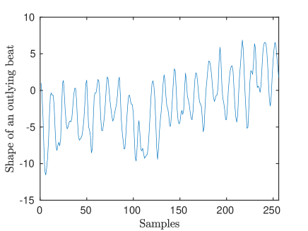
Figure 4: Histogram of $k$ values for approximating (up to ${\mathrm{prdn}}=9$) the ${\tt{N}}$-signals in the training set (left graph). Signal corresponding to the outlying value $k=63$ (right graph).

Even if not very noticeable in the histogram there are a few values of $k$ very far from the main support. These values are from ‘rare’ signals that should be investigated. In this set they are just signals looking as pure noise, e.g. the signal in the right graph of Fig 4 corresponds to $k=61$, very far from the mean value, $\overline{k}=14.31$ with standard deviation ${\mathrm{std}}=5.90$. When learning the dictionary for classification of ${\tt{N}}$ beats we disregard beats in the training set producing values of $k$ outside the range $(\overline{k}-3\,{\mathrm{std}},\overline{k}+3\,{\mathrm{std}})$. This amounts to disregarding $2.58\%$ of the total ${\tt{N}}$ beats in the training set set.

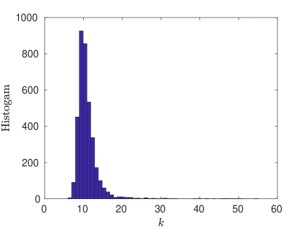
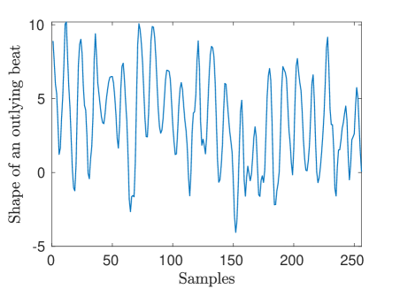
Figure 5: Histogram of $k$ values for approximating (up to ${\mathrm{prdn}}=9$) the ${\tt{V}}$-signals in the training set (left graph). Signal corresponding the outlying value $k=41$ (right graph).

The left graph of Fig.4 shows the histograms of $k$ values obtained when approximating, up to ${\mathrm{prdn}}=9$, the ${\tt{V}}$ beats in the training set of the numerical Test I. For this class $\overline{k}=10.61$ with ${\mathrm{std}}=3.28$. Because the data set of ${\tt{V}}$ beats is smaller than the previous one, when learning the dictionary for classification of ${\tt{V}}$ beats we disregard beats in the training set outside the range $(\overline{k}-2\,{\mathrm{std}},\overline{k}+2\,{\mathrm{std}})$. This amounts to disregarding $2.65\%$ of the ${\tt{V}}$ beats in the training set.

3.1 Numerical Test I

The purpose of this test is to assess the suitability of binary morphological differentiation of heartbeats using dictionaries learned from examples of ${\tt{N}}$ and ${\tt{V}}$ shapes in the dataset. For this end we randomly split the $Q=89840$ ${\tt{N}}$ beats into two groups: 35% of the ${\tt{N}}$ beats, are used for training the dictionary, $\mathbf{D}_{n}$ say. The remaining 65% of the ${\tt{N}}$ beats are reserved for testing. Since the ${\tt{V}}$ beats are much less than the ${\tt{N}}$ ones, $50\%$ of the ${\tt{V}}$ beats are used for training the dictionary $\mathbf{D}_{v}$, and the remaining $50\%$ for testing (c.f. Table 1)

Sets	Training		Testing
Class	${\tt{N}}$	${\tt{V}}$	${\tt{N}}$	${\tt{V}}$
Number of beats	30000	3359	57277	3359

Table 1: Number of heartbeats of classes ${\tt{N}}$ and ${\tt{V}}$ in the training and testing sets for Test I.

The dictionaries are learned to have redundancy two, i.e. each dictionary is a matrix of real numbers of size $256\times 512$. We test the method against:
(i) The initial dictionary.
(ii) The different greedy algorithms considered in this work: MP, OMP, OOMP.

For this test we randomly take 512 beats from the $30000$ ${\tt{N}}$ heartbeats in the training set to construct a matrix $\mathbf{D}_{n}$ of size $256\times 512$, which is used as initial dictionary. The learning curves for the dictionary $\mathbf{D}_{n}$ with the 3 greedy algorithms are shown in left graph of Fig.6. We repeat the process but taking the 512 dictionary atoms randomly from the $3358$ ${\tt{V}}$ beats in the training set. The learning curves for this dictionary are shown in the right graph of Fig.6.

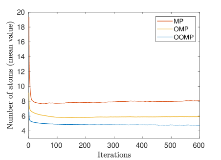
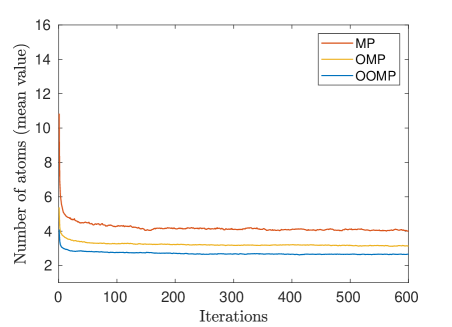
Figure 6: Dictionary learning curves with the tree greedy algorithms. The left graph corresponds to dictionary $\mathbf{D}_{n}$ and the right graph to dictionary $\mathbf{D}_{v}$.

The classification performance is assessed by means of the true positive (TP), false positive (FP), and false negative (FN) outcomes. These values are used to calculate the following statistics metrics for each class.

Sensitivity ($\mathrm{SE}$): Number of correctly classified heartbeats among the total number of beats in the set, i.e.

$$\mathrm{SE}=\frac{\mathrm{TP}}{\mathrm{TP}+\mathrm{FN}}.$$

Positive predictivity (PP): Ratio of correctly classified heartbeats to all the beats classified in that class.

$$\mathrm{PP}=\frac{\mathrm{TP}}{\mathrm{TP}+\mathrm{FP}}.$$

Additionally, the total accuracy ($\mathrm{AC}$) of the classification is calculated as the fraction of correctly classified heartbeats in both classes

$$\mathrm{AC}=\frac{\text{Correctly classified beats in both classes}}{\text{Total number of beats}}.$$

In Table 2 these scores are given as the mean value of 5 realisations corresponding to 5 random initialisations in the dictionary learning process. The standard deviations (std) are shown in rows 4,6,8,10, and 12 of Table 2. The Matlab codes for implementing the approach with the all the tree greedy algorithms have been made available on [28].

	MP				OMP				OOMP
Crit.	I (a)	I (b)	II	III	I (a)	I (b)	II	III	I (a)	I (b)	II	III
$\mathrm{SE}_{{\tt{N}}}$ (%)	99.7	99.7	99.7	99.7	99.1	99.1	99.3	99.4	98.8	98.8	98.5	97.4
std	0.05	0.05	0.04	0.03	0.09	0.09	0.01	0.04	0.14	0.13	0.16	0.45
$\mathrm{SE}_{{\tt{V}}}$ (%)	95.7	95.7	96.9	97.6	96.5	96.5	96.7	97.0	97.6	97.6	97.3	95.3
std	0.65	0.63	0.45	0.34	0.24	0.18	0.27	0.25	0.35	0.21	0.47	1.17
$\mathrm{PP}_{{\tt{N}}}$ (%)	99.7	99.7	99.8	99.9	99.8	99.8	99.8	99.8	99.9	99.9	99.8	99.7
std	0.04	0.04	0.03	0.02	0.01	0.01	0.02	0.01	0.02	0.01	0.03	0.07
$\mathrm{PP}_{{\tt{V}}}$ (%)	94.9	94.9	94.6	94.1	86.4	86.6	88.6	90.4	82.5	82.5	79.5	68.4
std	0.71	0.71	0.55	0.48	1.27	1.27	0.17	0.55	1.56	1.72	1.72	3.48
$\mathrm{AC}$ (%)	99.5	99.5	99.5	99.5	99.0	99.0	99.1	99.3	98.7	98.7	98.5	97.3
std	0.03	0.03	0.02	0.03	0.01	0.01	0.02	0.05	0.12	0.13	0.12	0.38

Table 2: Average statistics scores (of 5 different initialisations in the dictionary learning procedure) for classes ${\tt{N}}$ and ${\tt{V}}$, obtained with MP, OMP, and OOMP, and the sparsity criteria discussed in Sec. 2.2. std indicates the corresponding standard deviations and $\mathrm{AC}$ the average accuracy.

Discussion of results

i) The high accuracy and $\mathrm{SE}$ values for both classes, indicates that: 35% of the whole ${\tt{N}}$ beats in the data set and 50% of the whole ${\tt{V}}$ beats in the data set provide enough examples in the training set to learn dedicated dictionaries for each class.

ii) From Table I we can assert that each of the greedy algorithms performs better with a particular decision criterion.

iii) MP, combined with the decision Criterion II (norm-1), produces the highest statistics scores.

iv) For most of the scores, the random initialisation of the learning process does not change the results in any significant manner (low std values).

v) The comparatively much lower values of $\mathrm{PP}_{{\tt{V}}}$ reflex the enormous difference of the number of ${\tt{N}}$ and ${\tt{V}}$ beats in the testing sets (57277 vs 3359 beats). Hence, even if the percentage of incorrectly classified ${\tt{N}}$ beats is small, the classification being binary implies that the number of incorrectly classified ${\tt{N}}$ beats count as false positive ${\tt{V}}$. This causes the low $\mathrm{PP}_{{\tt{V}}}$ values in comparison to the other statistics metrics.

vi) Even if the OOMP approach secures the least number of atoms in th learning process (c.f. Fig.6) it is not the approach rendering the highest classification scores. This is because what matters for classification is the relative sparsity with respect to the 2 dictionaries. It is not surprising, though, that OOMP is the only approach that works better with Criterion I.

Remark 4.

Accuracy of 99% for differentiating classes in the whole MIT-BIH Arrhythmia data set is state of the art result obtainable from other features and other machine learning classifiers. See for instance

• $\mathrm{AC}\,\,99\%$for classification of 2 classes,

• $\mathrm{AC}\,\,99\%$ for classification of 5 classes,

• $\mathrm{AC}\,\,99.2\%$ for classification of 16 classes,

• $\mathrm{AC}\,\,99.3\%$ for classification of 16 classes.

Although results are not strictly comparable, because the number of classes are different, we believe it appropriate to highlight that the 99.5% accuracy attained in this work achieves equivalent values as other approaches do for binary and multi classification.

3.2 Test II

We test now the proposal in a more challenging situation. Because the morphology of ${\tt{N}}$ and ${\tt{V}}$ depends on the particular ECG signal, a realistic test is carried out by taking the training set and testing set from different records (corresponding to different patients).

Following previous publications [22, 13] the data are divided for training and testing as below.

The training set is taken only from the 21 records below in the the MIT-BIH Arrhythmia data set.

101, 106, 108, 112, 114, 115, 118, 119, 122, 124, 201, 203, 205, 207, 208, 209, 215, 220, 223, 230.

The remaining 21 records provide the testing set. These are the records

100, 103, 105, 111, 113, 117, 121, 123, 200, 202, 210, 212, 213, 214, 219, 221, 222, 231, 232, 233, 234 in the MIT-BIH Arrhythmia data set.

	MP				OMP				OOMP
Crit.	I (a)	I (b)	II	III	I (a)	I (b)	II	III	I (a)	I (b)	II	III
$\mathrm{SE}_{{\tt{N}}}$ (%)	89.8	89.9	90.5	91.8	88.8	89.5	88.8	92.5	88.7	89.0	85.7	81.5
std	1.43	1.39	1.38	1.26	1.39	1.28	1.48	1.19	0.92	0.87	0.98	2.10
$\mathrm{SE}_{{\tt{V}}}$ (%)	87.6	87.6	90.2	91.0	89.8	89.5	90.5	88.9	92.3	92.6	89.6	84.7
std	1.57	1.64	0.75	1.14	1.40	1.24	1.46	1.14	0.76	0.94	1.15	2.83
$\mathrm{PP}_{{\tt{N}}}$ (%)	99.0	99.0	99.2	99.3	99.2	99.2	99.2	99.1	99.4	99.4	99.1	98.7
std	0.11	0.12	0.05	0.08	0.11	0.09	0.11	0.08	0.06	0.07	0.10	0.22
$\mathrm{PP}_{{\tt{V}}}$	38.8	39.1	41.1	45.1	37.1	38.5	37.3	46.6	37.5	38.2	31.5	25.2
std	3.01	2.96	3.30	3.56	2.70	2.70	2.73	4.10	1.96	1.85	1.47	1.69
$\mathrm{AC}$	89.7	89.8	90.4	91.8	88.9	89.5	88.9	92.2	89.0	89.3	86.0	81.7
std	1.25	1.21	1.24	1.10	1.24	1.14	1.33	1.08	0.84	0.79	0.91	1.81

Table 3: Same description as in Table 2 but for the numerical Test II, in which training and testing sets correspond to different records.

Discussion of results

i) As expected, the classifications scores are lower than in Test I. This is because not all the shapes of the beats in the testing set bears similarity with shapes present in the training set.

ii) Also in this test each of the greedy algorithms performs better with a particular decision criterion.

iii) The greedy algorithm OOMP is the only one that performs better with Criterion I.

iv) Clearly MP works best with Criterion III and for most scores OMP as well.

v) The low values of $\mathrm{PP}_{{\tt{V}}}$ have the same cause as in Test I. Here all values are even lower because the incorrectly classified ${\tt{N}}$ beats are more than in Test I.

Remark 5.

In order to put the results into context we give here some indication of other technique performance. Nonetheless, it should be stressed once again that scores are not strictly comparable due to difference in the number of classes and, for the binary case, the classes and records for learning and testing.

• $\mathrm{AC}\,\,97\%$ for binary classification with 37 records for training and 11 records for testing, two of which are from a different data set.

• $\mathrm{AC}\,\,86.7\%$ for classification of 4 classes.

• $\mathrm{AC}\,\,89.18\%$ for classification of 5 classes.

• $\mathrm{AC}\,\,89.93\%$ classification in of 5 classes.

4 Conclusions

A set up for binary morphological identification of heartbeats on the basis of sparsity metrics has been laid out. The proposal was tested for identification of ${\tt{N}}$ and ${\tt{V}}$ beats in the MIT-BIH Arrhythmia data set, achieving state of the art scores.

Because the number of ${\tt{N}}$ and ${\tt{V}}$ beats in the MIT-BIH Arrhythmia are unbalanced, the $\mathrm{AC}$ score is not reliable for assessment. Nevertheless, the percentage of correctly classified ${\tt{N}}$ and ${\tt{V}}$ are similar to the $\mathrm{AC}$ score in both numerical tests.

The results are encouraging because the proposed binary identification is realised outside the usual machine leaning framework, using sparsity as a single parameter for making a decision. Thus, extensions of the approach to allow for combination with other features and other machine leaning techniques are readily foreseen.

The possibility of implementing the technique depends on the availability of ‘enough’ examples to learn the corresponding dictionaries. In the numerical tests realised here, for instance, 3359 examples for beats ${\tt{V}}$ were enough to learn the dictionary $\mathbf{D}_{v}\in\mathbb{R}^{256\times 512}$.

References

- [1] U. R. Acharya, Shu Lih Oh, Y. Hagiwara, Jen Hong Tan, M. Adam, A. Gertych, Ru San Tan, “A deep convolutional neural network model to classify heartbeats”, Computers in Biology and Medicine, 89 389–396 (2017).
- [2] A. Mincholé and B. Rodriguez, “Artificial intelligence for the electrocardiogram” Nature Medicine, 25, 22–23 (2019) https://doi.org/10.1038/s41591-018-0306-1
- [3] A. Y. Hannun, P. Rajpurkar, M. Haghpanahi, G. H. Tison, C. Bourn, M. P. Turakhia, and A. Y. Ng, “Cardiologist-level arrhythmia detection and classification in ambulatory electrocardiograms using a deep neural network”, Nature Medicine, 25, 65–69 (2019).
- [4] A. H. Ribeiro, M. H. Ribeiro, G. M. M. Paixão, D. M. Oliveira, P. R. Gomes, J. A. Canazart, M. P. S. Ferreira, C. R. Andersson, P. W. Macfarlane, W Meira Jr., T. B. Schön, and A. L. P. Ribeiro, “Automatic diagnosis of the 12-lead ECG using a deep neural network”, Nature Communications, 11, 1760 (2020) https://doi.org/10.1038/s41591-018-0268-3.
- [5] Y. LeCun, Y. Bengio, and G. Hinton, , “Deep learning”. Nature 521, 436–444 (2015).
- [6] X. Han, Y. Hu, L. Foschini, L. Chinitz, L. Jankelson, and R. Ranganath, “ Deep learning models for electrocardiograms are susceptible to adversarial attack Nature Medicine, 26,360–363 (2020).
- [7] L. Ma and L. Liang, “A regularization method to improve adversarial robustness of neural networks for ECG signal classification”, Computers in Biology and Medicine 144, (2020) https://doi.org/10.1016/j.compbiomed.2022.105345.
- [8] E. J. Luz, W. R. Schwartz, G. Cámara-Chávez, and, D. Mennotti, ECG-based heartbeat classification for arrhythmia detection: A survey, Computer Methods and Programs in Biomedicine 127, 144–164 (2016) doi: https://doi.org/10.1016/j.cmpb.2015.12.008.
- [9] U.R. Acharya, H. Fujita, M. Adam, S.L. Oh, K.V. Sudarshan, J.H. Tan, J.E.W. Koh, Y. Hagiwara, C.K. Chua, C.K. Poo, and R.S. Tan, Automated characterization and classification of coronary artery disease and myocardial infarction by decomposition of ECG signals: A comparative study, Information Sciences, 377 (2017) 17–29. doi:https://doi.org/10.1016/j.ins.2016.10.013.
- [10] A. Lyon , A. Mincholé, J. P. Martínez, P. Laguna, B. Rodriguez, Computational techniques for ECG analysis and interpretation in light of their contribution to medical advances, Journal of the Royal Society of Interface,15 (2018), article No. 20170821 https://doi.org/10.1098/rsif.2017.0821.
- [11] E. Merdjanovska and A. Rashkovska, “Comprehensive survey of computational ECG analysis: Databases, methods and applications”, Expert Systems With Applications 203, 117206 (2022).
- [12] J. Wright, A. Y. Yang, A. Ganesh, S. S, Sastry, and Yi Ma, “Robust Face Recognition via Sparse Representation”, IEEE Trans. on Pattern Analysis and Machine Intelligence, 31, 210–227 (2008).
- [13] S. Raj and K. Ch. Ray, “Sparse representation of ECG signals for automated recognition of cardiac arrhythmias”, Expert Systems with Applications, 105, 49–65 (2018).
- [14] S.S. Chen, D.L. Donoho, and M.A. Saunders. Atomic decomposition by basis pursuit. SIAM Journal on Scientific Computing, 20, 33–61 (1998).
- [15] S. G. Mallat and Z. Zhang, “Matching Pursuits with Time-Frequency Dictionaries”, IEEE Trans. on Signal Processing, 41, 3397–3415 (1993).
- [16] Y.C. Pati, R. Rezaiifar, and P.S. Krishnaprasad, “Orthogonal matching pursuit: recursive function approximation with applications to wavelet decomposition,” Proceedings of the 27th Annual Asilomar Conference in Signals, System and Computers, 1, 40–44, (1993).
- [17] L. Rebollo-Neira and D. Lowe, “Optimised orthogonal matching pursuit approach”, IEEE Signal Process. Letters, 9, 137–140 (2002).
- [18] L. Rebollo-Neira, M. Rozložník, and P. Sasmal, “Analysis of the Self Projected Matching Pursuit Algorithm”, Journal of The Franklin Institute, 357, 8980–8994 (2020).
- [19] https://physionet.org/physiobank/database/mitdb/ (Last access Jan 2023).
- [20] G. B. Moody, R. G. Mark, “The impact of the MIT-BIH Arrhythmia Database”, IEEE Eng in Med and Biol, 20, 45–50 (2001)..
- [21] A. Goldberger, L. Amaral, L. Glass, J. Hausdorff, P. C. Ivanov, R. Mark, J.E. Mietus, G. B. Moody, C. K. Peng, and H. E. Stanley, “PhysioBank, PhysioToolkit, and PhysioNet: Components of a new research resource for complex physiologic signals.” Circulation [Online]. 101 e215–-e220 (2000).
- [22] P. de Chazal, M. O’Dwyer and R. B. Reilly, “Automatic Classification of Heartbeats Using ECG Morphology and Heartbeat Interval Features”, IEEE Trans. on Biomedical Engineering, 51, 1196–1206 (2004)
- [23] R. R. Coifman and M. V. Wickerhauser, “Entropy-based algorithms for best basis selection”, IEEE Trans. on Information Theory 38, 713 –718 (1992).
- [24] M. Andrle and L. Rebollo-Neira, From cardinal spline wavelet bases to highly coherent dictionaries, Journal of Physics A 41 (2008), article No. 172001. doi:10.1088/1751-8113/41/17/172001.
- [25] L. Rebollo-Neira, D. Černá, “Wavelet based dictionaries for dimensionality reduction of ECG signals”, Biomedical Signal Processing and Control, 54 (2019), article No. 101593. doi:https://doi.org/10.1016/j.bspc.2019.101593.
- [26] D. Černá and L. Rebollo-Neira, “Construction of wavelet dictionaries for ECG modeling” MethodsX, 8, 101314 (2021).
- [27] http://www.nonlinear-approx.info/examples/node013.html
- [28] http://www.nonlinear-approx.info/examples/node016.html
- [29] R. J. Martis, U. R. Acharya, H. Prasad, K. C. Chua, and C. M. Lim, “Automated detection of atrial fibrillation using Bayesian paradigm,” Knowledge-Based Syst., 54, 269–275 (2013).
- [30] E. Alickovic and A. Subasi, “Effect of Multiscale PCA De-noising in ECG Beat Classification for Diagnosis of Cardiovascular Diseases”, Circuits, Systems, and Signal Processing, 34 513–533 (2015).
- [31] S. Raj, K. C. Ray, and O. Shankar, “Cardiac arrhythmia beat classification using DOST and PSO tuned SVM”, Computer Methods and Programs in Biomedicine, 136, 163–177 (2016).
- [32] F. I. Alarsan and M. Younes, “Analysis and classification of heart diseases using heartbeat features and machine learning algorithms”, Journal of Big Data, (2019) https://doi.org/10.1186/s40537-019-0244-x.
- [33] Z. Zhang, J. Dong, X. Luo, Kup-Sze Choi, X. Wu, “Heartbeat classification using disease-specific feature selection”, Computers in Biology and Medicine, 46, 79–89 (2014).