Inference via robust optimal transportation: theory and methods

Abstract

Optimal transport (OT) theory and the related $p$-Wasserstein distance ($W_{p}$, $p\geq 1$) are widely-applied in statistics and machine learning. In spite of their popularity, inference based on these tools is sensitive to outliers or it can perform poorly when the underlying model has heavy-tails. To cope with these issues, we introduce a new class of procedures. (i) We consider a robust version of the primal OT problem (ROBOT) and show that it defines the robust Wasserstein distance, $W^{(\lambda)}$, which depends on a tuning parameter $\lambda>0$. (ii) We illustrate the link between $W_{1}$ and $W^{(\lambda)}$ and study its key measure theoretic aspects. (iii) We derive some concentration inequalities for $W^{(\lambda)}$. (iii) We use $W^{(\lambda)}$ to define minimum distance estimators, we provide their statistical guarantees and we illustrate how to apply concentration inequalities for the selection of $\lambda$. (v) We derive the dual form of the ROBOT and illustrate its applicability to machine learning problems (generative adversarial networks and domain adaptation). Numerical exercises provide evidence of the benefits yielded by our methods.

Keywords: Minimum distance estimation, Robust Wasserstein distance, Robust generative adversarial networks

1 Introduction

1.1 Related literature

OT formulation dates back to the early work of Monge (1781) , who considered the problem of finding the optimal way to move given piles of sand to fill up given holes of the same total volume. Monge’s problem remained open until the 1940s, when it was revisited and solved by Kantorovich, in relation to the economic problem of optimal allocation of resources. We refer to Villani (2009), Santambrogio (2015) for a book-length presentation in mathematics, to Peyré and Cuturi (2019) for a data science view, and to Panaretos and Zemel (2020) for a statistical perspective.

Within the OT setting, the Wasserstein distance ($W_{p},p\geq 1$) is defined as the minimum cost of transferring the probability mass from a source distribution to a target distribution, for a given transfer cost function. Nowadays, OT theory and $W_{p}$ are of fundamental importance for many scientific areas, including statistics, econometrics, information theory and machine learning. For instance, in machine learning, OT based inference is a popular tool in generative models; see e.g. Arjovsky et al. (2017), Genevay et al. (2018), Nietert et al. (2022) and references therein. Similarly, OT techniques are widely-applied for problems related to domain adaptation; see Courty et al. (2014) and Balaji et al. (2020). In statistics and econometrics, estimation methods based on $W_{p}$ are related to minimum distance estimation (MDE); see Bassetti et al. (2006) and Bernton et al. (2019). MDE is a research area in continuous development and the estimators based on this technique are called minimum distance estimators. They are linked to M-estimators and may be robust. We refer to Hampel et al. (1986), Van der Vaart (2000) and Basu et al. (2011) for a book-length statistical introduction. As far as econometrics is concerned, we refer to Kitamura and Stutzer (1997) and Hayashi (2011). The extant approaches for MDE are usually defined via Kullback-Leibler (KL) divergence, Cressie-Read power divergence, Jensen-Shannon distance, total variation (TV) distance, Kolmogorov-Sminrov distance, Hellinger distance, to mention a few. Some of those approaches (e.g. Hellinger distance) require kernel density estimation of the underlying probability density function (pdf). Some of others (e.g. KL divergence) have poor performance when the considered distributions do not have a common support. Compared to other notions of distance or divergence, $W_{p}$ avoids the mentioned drawbacks, e.g. it can be applied when the considered distributions do not share the same support and inference is conducted in a generative fashion—namely, a sampling mechanism is considered, in which non-linear functions map a low dimensional latent random vector to a larger dimensional space; see Genevay et al. (2018). This explains why $W_{p}$ is becoming a popular inference tool; see e.g. Courty et al. (2014); Frogner et al. (2015); Kolouri et al. (2017); Carriere et al. (2017); Peyré and Cuturi (2019) and Hallin (2022); La Vecchia et al. (2022) for an overview of technology transfers among different areas.

In spite of their appealing theoretical properties, OT and $W_{p}$ have two important inference aspects to deal with: (i) implementation cost and (ii) lack of robustness. (i) The computation of the solution to OT problem and of the $W_{p}$ can be demanding. To circumvent this problem, Cuturi (2013) proposes the use of an entropy regularized version of the OT problem. The resulting divergence is called Sinkhorn divergence; see Amari et al. (2018) for further details. Genevay et al. (2018) illustrate the use of this divergence for inference in generative models, via MDE. The proposed estimation method is attractive in terms of performance and speed of computation. However (to the best of our knowledge) the statistical guarantees of the minimum Sinkhorn divergence estimators have not been provided. (ii) Robustness is becoming a crucial aspect for many complex statistical and machine learning applications. The reason is essentially two-fold. First, large datasets (e.g. records of images or large-scale data collected over the internet) can be cluttered with outlying values (e.g. due to measurement errors or recording device failures). Second, every statistical model represents only an approximation to reality. Thus, one needs to devise inference procedures that remain informative even in the presence of small deviations from the assumed statistical (generative) model. Robust statistics deals with this problem. We refer to Hampel et al. (1986) and Ronchetti and Huber (2009) for a book-length discussion on robustness principles.

Other papers have already mentioned the robustness issues of $W_{p}$ and OT; see e.g. Alvarez-Esteban et al. (2008), Hallin et al. (2020), del Barrio et al. (2022), Mukherjee et al. (2021), Yatracos (2022) and Ronchetti (2022). In the OT literature, Chizat (2017) proposes to deal with outliers via unbalanced OT, namely allowing the source and target distribution to be non-standard probability distributions. Working along the lines of unbalanced OT theory, Balaji et al. (2020) define a robust optimal transportation (ROBOT) problem, which is based on the solution of a penalized OT problem. Similarly, starting from OT formulation with a regularization term, Mukherjee et al. (2021) derive a novel robust OT problem, that they label as ROBOT. Moreover, building on the Minimum Kantorovich Estimator (MKE) of Bassetti et al. (2006), Mukherjee et al. propose a class of estimators obtained through minimizing the ROBOT and illustrate numerically their performance. Finally, we mention that Nietert et al. (2022) recently defined a notion of outlier-robust Wasserstein distance which allows for a percentage of outlier mass to be removed from contaminated distributions.

1.2 Our contributions

Working at the intersection between of the mentioned streams of literature, we study the theoretical, methodological and computational aspects of ROBOT. Our contributions can be summarized as follows.

We prove that the primal ROBOT problem of Mukherjee et al. (2021) defines a robust distance that we call robust Wasserstein distance $W^{(\lambda)}$, which depends on a tuning parameter $\lambda$ controlling the level of robustnes. We study the measure theoretic properties of $W^{(\lambda)}$, proving that it induces a metric space whose separability and completeness are proved. Moreover, we derive concentration inequalities for the robust Wasserstein distance and illustrate their practical applicability for the selection of $\lambda$ in the presence of outliers.

These theoretical findings are instrumental to another contribution of this paper: the development of a novel inferential theory based on robust Wasserstein distance. Hinging on convex analysis (Rockafellar and Wets, 2009) and using the techniques of Bernton et al. (2019), we prove that the minimum robust Wasserstein distance estimators exist (almost surely) and are consistent (at the reference model, possibly misspecified). Numerical experiments show that the robust Wasserstein distance estimators remain reliable even in the presence of local departures from the postulated statistical model. These results complete the methodological investigations already available in the literature on MKE (Bassetti et al. (2006) and Bernton et al. (2019)) and on ROBOT (Balaji et al. (2020) and Mukherjee et al. (2021)). Indeed, beside the numerical evidence, in the literature there are (to the best of our knowledge) no statistical guarantees on the estimators obtained by the method of Mukherjee et al. (2021) and Balaji et al. (2020). As far as the approach in Nietert et al. (2022) is concerned, we remark that their notion of robust Wasserstein distance has a similar spirit to our $W^{(\lambda)}$ (both are based on a total variation penalization of the original OT problem, but yield different duality forumulations) and, similarly to our results in §5.3, it is proved to be useful in generative adversarial network (GAN). In spite of these similarities, our investigation goes deeper in the inferential aspects and statistical use of $W^{(\lambda)}$. Indeed, Nietert et al. do study concentration inequalities for their distance and not define the estimators related to the minimization of their outlier-robust Wasserstein distance.

Another contribution of our paper is the derivation of the dual form of ROBOT for application to machine learning problems. This result not only completes the theory available in Mukherjee et al. (2021), but also provides the stepping stone for the implementation of ROBOT. We explain how our duality can be applied to define robust Wasserstein Generative Adversarial Networks (RWGAN). Numerical exercises illustrate that RWGAN have better performance than the routinely-applied Wasserstein GAN (WGAN) models; see Algorithm 2 in Appendix C.2 for the computational details. Moreover, we illustrate how to use ROBOT for outlier detection in domain adaptation, another machine learning problem; see Appendix E for the algorithm (Algorithm 3) and for numerical experiments.

1.3 Structure of the paper

We organize our material as follows. In Section 2, we review briefly the classical OT and introduce ROBOT (in its primal and dual formulation). In Section 3, based on ROBOT, we define $W^{(\lambda)}$, we study its relevant theoretical properties and we derive concentration inequalities. In Section 4, we define minimum robust Wasserstein distance estimators and we establish their asymptotics. Monte Carlo experiments and real data analysis, illustrating the applicability of the ROBOT to statistical inference and machine learning problems, are given in Section 5. In Section 6 we discuss a selection procedure for the tuning parameter controlling ROBOT. The Supplementary Material contains several appendices which include some key results on optimal transport, proofs, algorithms needed to implement our methods, additional Monte Carlo exercises and details about the $\lambda$ selection procedure. The codes to reproduce our results are available at the Authors GitHub space.

2 Optimal transport

We recall the fundamental notions of OT as in Villani (2009) and of ROBOT, as defined in Mukherjee et al. (2021). Throughout this paper, $\mathcal{X}$ and $\mathcal{Y}$ denote two Polish spaces, and $\mathcal{P}(\mathcal{X})$ represents the set of all probability measures on $\mathcal{X}$.

2.1 Classical OT

Let $\Pi(\mu,\nu)$ denote the set of all joint probability measures of $\mu\in\mathcal{P(X)}$ and $\nu\in\mathcal{P(Y)}$. Kontorovich’s problem aims at finding a joint distribution $\pi\in\Pi(\mu,\nu)$ which minimizes the expectation of the coupling between $X$ and $Y$ in terms of the cost function $c$. This problem can be formulated as

$$\inf\left\{\int_{\mathcal{X\times Y}}c(x,y)d\pi(x,y):\pi\in\Pi(\mu,\nu)\right\}.$$ (1)

A solution to Kantorovich’s problem (KP) (1) is called an optimal transport plan. Note that Kantorovich’s problem is convex, and the solution to (1) exists under some mild assumptions on $c$, e.g., lower semicontinuous; see e.g. Villani (2009, Chapter 4).

KP as in (1) has a dual form, which is related to solving the Kantorovich dual (KD) problem

$$\sup\left\{\int_{\mathcal{Y}}\phi d\nu-\int_{\mathcal{X}}\psi d\mu:\phi\in C_{b}(\mathcal{Y}),\psi\in C_{b}(\mathcal{X})\right\}\quad\text{s.t.}\quad\phi(y)-\psi(x)\leq c(x,y),\enspace\forall(x,y),$$

where $C_{b}(\mathcal{X})$ is the set of bounded continuous functions on $\mathcal{X}$—additional details are available in the Supplementary Material. According to Th. 5.10 in Villani (2009), if function $c$ is lower semicontinuous, there exists a solution to the dual problem such that the solutions to KD and KP coincide (no duality gap). In this case, the solution takes the form

$$\phi(y)=\inf\limits_{x\in\mathcal{X}}[\psi(x)+c(x,y)]\quad\text{and}\quad\psi(x)=\sup\limits_{y\in\mathcal{Y}}[\phi(y)-c(x,y)],$$

where the functions $\phi$ and $\psi$ are called $c$-concave and $c$-convex, respectively, and $\phi$ (resp. $\psi$) is called the $c$-transform of $\psi$ (resp. $\phi$). A special case is that when $c$ is a metric on $\mathcal{X}$, thus OT problem becomes $\sup\left\{\int_{\mathcal{X}}\psi d\nu-\int_{\mathcal{X}}\psi d\mu:\psi\,\text{is 1-Lipschitz continuous}\right\}.$ This case is commonly known as Kantorovich-Rubenstein duality.

Let $(\mathcal{X},d)$ denote a complete metric space equipped with a metric $d:\mathcal{X}\times\mathcal{X}\rightarrow\mathbb{R}$, and let $\mu$ and $\nu$ be two probability measures on $\mathcal{X}$. Solving the optimal transport problem in (1), with the cost function $c(x,y)=d^{p}(x,y)$, introduces a distance, called Wasserstein distance, between $\mu$ and $\nu$. More specifically, the Wasserstein distance of order $p$ $(p\geq 1)$ is

$$W_{p}(\mu,\nu) =\left(\inf\int_{\mathcal{X\times X}}(d(x,y))^{p}d\pi(x,y)\right)^{1/p}.$$ (2)

For the interested reader, Appendix A recalls some key results on optimal transport.

Remark. The ability to lift the ground distance $d(x,y)$ is one of the perks of $W_{p}$ and it makes it a suitable tool in statistics and machine learning; see Remark 2.18 in Peyré and Cuturi (2019). Interestingly, this desirable feature becomes a negative aspect as far as robustness is concerned. Intuitively, OT embeds the distributions geometry: when the underlying distribution is contaminated by outliers, the marginal constraints force OT to transport outlying values, inducing an undesirable extra cost, which in turns entails large changes in the $W_{p}$. More in detail, let $\delta_{x_{0}}$ be point mass measure centered at $x_{0}$ (a point in the sample space), and $d(x,y)$ be the ground distance. Then, we introduce the $O\cup I$ framework, in which the majority of the data $(X_{i})_{i\in I}$ are inliers, that is i.i.d. informative data with distribution $\mu$, whilst a few data $(X_{i})_{i\in O}$ are outliers, meaning that they are not i.i.d. with distribution $\mu$. We refer to Lecué and Lerasle (2020) (and references therein) for more detail on $O\cup I$ and for discussion on its connection to Huber gross-error neighbourhood. Thus, for $\varepsilon>0$, we have $W_{p}({\rm\mu},(1-\varepsilon){\rm\mu}+\varepsilon\delta_{x_{0}})\rightarrow\infty$, as $x_{0}\rightarrow\infty$. Thus, $W_{p}$ can be arbitrarily inflated by a small number of large observations and it is sensitive to outliers. For instance, let us consider $W_{p}$, with $p=1,2$. In Figure 1(a) and 1(b), we display the scatter plot for two bivariate distributions: the distribution in panel (b) has some abnormal points (contaminated sample) compared to the distribution in panel (a) (clean sample). Although only a small fraction of the sample data is contaminated, both $W_{1}$ and $W_{2}$ display a large increase. Anticipating some of the results that we will derive in the next pages, we compute our $W^{(\lambda)}$ (see §3.1) and we notice that its value remains roughly the same in both panels.

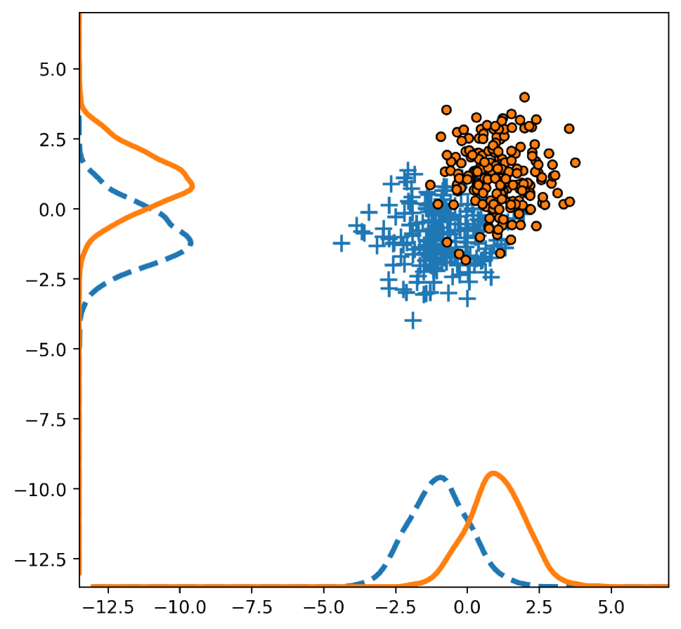
(a) $W_{1}=3.0073$, $W_{2}=3.0247$ and $W^{(\lambda)}=2.9324(\lambda=3)$

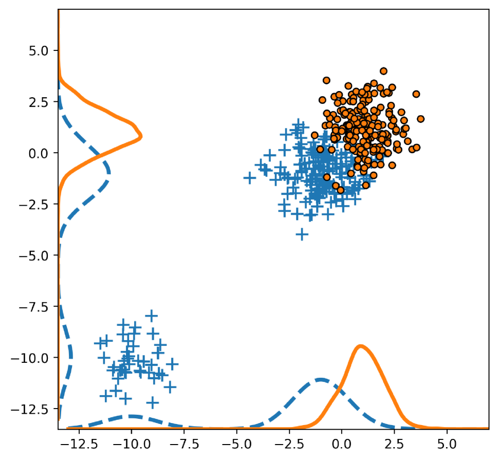
(b) $W_{1}=5.32491$, $W_{2}=6.6215$ and $W^{(\lambda)}=3.3142(\lambda=3)$

Figure 1: Wasserstein distance ($W_{1}$ and $W_{2}$) and robust Wasserstein distance ($W^{(\lambda)}$) between two bivariate distributions. The scatter plot of data in panel (a) represents a sample from the reference model: cross points (blue) are generated from $\mathcal{N}\left(\binom{-1}{-1},I_{2}\right)$, points (orange) are generated from $\mathcal{N}\left(\binom{1}{1},I_{2}\right)$; whilst the plot in panel (b) contains some outliers: cross points (blue) are generated from $0.8\mathcal{N}\left(\binom{-1}{-1},I_{2}\right)+0.2\mathcal{N}\left(\binom{-9}{-9},I_{2}\right)$, points (orange) are generated from $\mathcal{N}\left(\binom{1}{1},I_{2}\right)$. The marginal distributions are on the $x$- and $y$-axis.

2.2 Robust OT (ROBOT)

2.2.1 Primal formulation

We recall the ROBOT problem as defined in Mukherjee et al. (2021), who introduce a modified version of Monge-Kantorovich OT problem. Mukherjee et al. work on the notion of unbalanced OT: they consider a TV-regularized OT re-formulation

$$\begin{array}[]{ll}&\min_{\pi,s}\iint c(x,y)\pi(x,y)dxdy+\lambda\|s\|_{\mathrm{TV}}\\ \text{s.t.}&\int\pi(x,y)dy=\mu(x)+s(x)\geq 0\\ &\int\pi(x,y)dx=\nu(y)\\ &\int s(x)dx=0,\end{array}$$ (3)

where $\lambda>0$ is a regularization parameter. In (3), the original source measure $\mu$ is modified by adding $s$ (nevertheless, the first and last constraints ensure that $\mu+s$ is still a valid probability measure). Intuitively, having $\mu(x)+s(x)=0$ means that $x\in{\cal X}$ has strong impact on the OT problem and hence can be labelled as an outlier. The outlier is eliminated from the sample, since the probability measure $\mu+s$ at this point is zero.

Mukherjee et al. (2021) prove that a simplified, computationally efficient formulation equivalent to (3) is

$$\inf\left\{\int_{\mathcal{X\times X}}c_{\lambda}(x,y)d\pi(x,y):\pi\in\Pi(\mu,\nu)\right\},$$ (4)

which has a functional form similar to (1), but the cost function $c$ is replaced by the trimmed cost function $c_{\lambda}=\min\left\{c,2\lambda\right\}$ that is bounded from above by $2\lambda$. Following Mukherjee et al. (2021), we call formulations (3) and (4) ROBOT.

2.2.2 Dual formulation

In this section, we drive the dual form of the ROBOT, which is not available in Mukherjee et al. (2021).

Theorem 1.

Let $\mu,\nu$ be probability measures in $\mathcal{P(X)}$, with $c_{\lambda}(x,y)$ as in (6). Then the c-transform of a c-convex function $\psi(x)$ is itself, i.e. $\psi^{c}(x)=\psi(x)$. Moreover, the dual form of ROBOT is related to the Kantorovich potential $\psi$, which is a solution to

$$\sup\left\{\int_{\mathcal{X}}\psi d\mu-\int_{\mathcal{X}}\psi d\nu:\psi\in C_{b}(\mathcal{X})\right\},$$ (5)

where $\psi$ satisfies $|\psi(x)-\psi(y)|\leq d(x,y)$ and $\mathrm{range}(\psi)\leq 2\lambda$.

Note that the difference between the dual form of OT and that of ROBOT is that the latter imposes a restriction on the range of $\psi$. Thanks to this, we may think of using the ROBOT in theoretical proofs and inference problems where the dual form of OT is already applied, with the advantage that ROBOT remains stable even in the presence of outliers. In the next sections, we illustrate these ideas.

3 Robust Wasserstein distance $W^{(\lambda)}$

We are now ready to define a novel concept of distance based on ROBOT.

3.1 Key notions

Setting $c(x,y)=d(x,y)$, (2) implies that the corresponding minimal cost $W_{1}(\mu,\nu)$ is a metric between two probability measures $\mu$ and $\nu$. A similar result can be obtained also in the ROBOT setting of (4), if the modified cost function takes the form

$$c_{\lambda}(x,y):=\min\left\{d(x,y),2\lambda\right\}.$$ (6)

Lemma 1.

Let $d(\cdot,\cdot)$ denote a metric on ${\cal X}$. Then $c_{\lambda}(x,y)$ in (6) is also a metric on ${\cal X}$.

Based on Lemma 1, we define the robust Wasserstein distance and prove that it is a metric on $\mathcal{P(X)}$.

Theorem 2.

For $c_{\lambda}(x,y),x,y\in{\cal X},$ defined in (6),

$$W^{(\lambda)}(\mu,\nu):=\inf\limits_{\pi\in\Pi(\mu,\nu)}\left\{\int_{\mathcal{X\times X}}c_{\lambda}(x,y)d\pi(x,y)\right\}$$ (7)

is a metric on $\mathcal{P(X)}$, and we call it robust Wasserstein distance.

It is worth noting that $W_{p}$ is well defined only if probability measures have finite $p$-th order moments. In contrast, thanks to the boundedness of the $c_{\lambda}$, our $W^{(\lambda)}$ in (7) can be applied to all probability measures, even those with infinite moments of any order. Making use of $W^{(\lambda)}$ we introduce the following

Definition 1 (Robust Wasserstein space).

A robust Wasserstein space is an ordered pair $(\mathcal{P(X)},W^{(\lambda)})$, where $\mathcal{P(X)}$ is the set of all probability measures on a complete separable metric space $\mathcal{X}$, and $W^{(\lambda)}$ defined in Theorem 2 is a (finite) distance on $\mathcal{P(X)}$.

3.2 Some measure theoretic properties

Equipped with Th. 2 and Definition 1, it is interesting to connect $W_{1}$ to $W^{(\lambda)}$, via the characterization of its limiting behavior as $\lambda\rightarrow\infty$. Since $W^{(\lambda)}$ is continuous and monotonically increasing with respect to $\lambda$, one can prove (via dominated convergence theorem) that its limit coincides with the Wasserstein distance of order $p=1$. Thus:

Theorem 3.

For any probability measures $\mu$ and $\nu$ in ${\cal P}({\cal X})$, $W^{(\lambda)}$ is continuous and monotonically non-decreasing with respect to $\lambda\in[0,\infty)$. Moreover, if $W_{1}(\mu,\nu)$ exists, we have $\lim_{\lambda\rightarrow\infty}W^{(\lambda)}(\mu,\nu)=W_{1}(\mu,\nu).$

Th. 3 has a two-fold implication: first, it shows that the $W^{(\lambda)}\leq W_{1}$; second, for large values of the regularization parameter, $W^{(\lambda)}$ and $W_{1}$ behave similarly. Another important property of $W^{(\lambda)}$ is that weak convergence is entirely characterized by convergence in the robust Wasserstein distance. More precisely, we have

Theorem 4.

Let $\left(\mathcal{X},d\right)$ be a Polish space. Then $W^{(\lambda)}$ metrizes the weak convergence in $\mathcal{P({X})}$. In other words, if $\left(\mu_{k}\right)_{k\in\mathbb{N}}$ is a sequence of measures in $\mathcal{P(X)}$ and $\mu$ is another measure in $\mathcal{P(X)}$, then the statements $\left(\mu_{k}\right)_{k\in\mathbb{N}}\,\,\text{converges weakly in}\,\,\mathcal{P(X)}\,\,\text{to}\,\,\mu$ and $W^{(\lambda)}\left(\mu_{k},\mu\right)\rightarrow 0$ are equivalent.

The next result follows immediately from Theorem 4.

Corollary 1 (Continuity of $W^{(\lambda)}$).

For a Polish space $(\mathcal{X},d)$, suppose that $\mu_{k}\,(resp.\,\nu_{k})$ converges weakly to $\mu\,(resp.\,\nu)$ in $\mathcal{P(X)}$ as $k\rightarrow\infty$. Then $W^{(\lambda)}(\mu_{k},\nu_{k})\rightarrow W^{(\lambda)}(\mu,\nu).$

Finally, we prove the separability and completeness of robust Wasserstein space, when $\mathcal{X}$ is separable and complete. To this end, we state

Theorem 5.

Let $\mathcal{X}$ be a complete separable metric space. Then the space $\mathcal{P(X)}$, metrized by the robust Wasserstein distance $W^{(\lambda)}$, is complete and separable. Moreover, the set of finitely supported measures with rational coefficients is dense in $\mathcal{P(X)}$.

3.3 Probabilistic aspects

3.3.1 Transportation inequalities: a Sanov’s type theorem

The previous results offer the toolkit needed to derive some concentration inequalities for $W^{(\lambda)}$ building on the extant results for $W_{1}$. To illustrate this aspect, let us consider the case of Talagrand transportation inequality. We recall that using $W_{p}$ as a distance between probability measures, transportation inequalities state that, given $\alpha>0$, a probability measure $\mu$ on $X$ satisfies $T_{p}(\alpha)$ if the inequality $W_{p}(\mu,\nu)\leq\sqrt{{2}H(\mu|\nu)/{\alpha}}$ holds for any probability measure $\nu$, with $H(\mu|\nu)$ being the Kullback-Leibler divergence. For $p=1$, it has been proven that $T_{1}(\alpha)$ is equivalent to the existence of a square-exponential moment; see e.g. Bolley et al. (2007). Now, note that, from Theorem 3, we have $W^{(\lambda)}\leq W_{1}$: we can immediately claim that if $T_{1}(\alpha)$ holds, then we have $W^{(\lambda)}(\mu,\nu)\leq\sqrt{{2}H(\mu\mid\nu)/{\alpha}}$. Thanks to this consideration, we state

Theorem 6.

Let $\mu$ be a probability measure on $\mathbb{R}^{d}$, which satisfies a $T_{1}(\alpha)$ inequality, and $\{X_{1},...,X_{n}\}$ be a random sample of independent variables, all distributed according to $\mu$; let also $\hat{\mu}_{n}:=n^{-1}\sum_{i=1}^{n}\delta_{X_{i}}$ be the associated empirical measure, where $\delta_{x}$ is the Dirac distribution with mass on $x\in\mathbb{R}^{d}$. Then, for any $d^{\prime}>d$ and $\alpha^{\prime}<\alpha$, there exists some constant $n_{0}$, depending only on $\alpha^{\prime},d^{\prime}$ and some square-exponential moment of $\mu$, such that for any $\varepsilon>0$ and $n\geq n_{0}\max\left(\varepsilon^{-\left(d^{\prime}+2\right)},1\right)$, we have ${\rm P}\left[W^{(\lambda)}\left(\mu,\hat{\mu}_{n}\right)>\varepsilon\right]\leq\exp\{-\frac{\alpha^{\prime}}{2}n\varepsilon^{2}\}.$

The proof follows along the lines as the proof of Th. 2.1 in Bolley et al. combined with Theorem 1 which yields

$$\mathrm{exp}\{-\frac{\alpha^{\prime}}{2}n\varepsilon^{2}\}\geq{\rm P}\left[W_{1}\left(\mu,\hat{\mu}_{n}\right)>\varepsilon\right]\geq{\rm P}\left[W^{(\lambda)}(\mu,\hat{\mu}_{n})>\varepsilon\right].$$ (8)

A remark is in order. The condition $n\geq n_{0}\max\left(\varepsilon^{-\left(d^{\prime}+2\right)},1\right)$ implies that Th. 6 has asymptotic nature. Nevertheless, Bolley et al. prove that ${\rm P}\left[W_{1}\left(\mu,\hat{\mu}_{n}\right)>\varepsilon\right]\leq C(\epsilon)\exp\{-\frac{\alpha^{\prime}}{2}n\varepsilon^{2}\}$ hods for any $n$ with $C(\epsilon)$ being a (large) constant depending on $\epsilon$. The argument in (8) implies ${\rm P}\left[W^{(\lambda)}\left(\mu,\hat{\mu}_{n}\right)>\varepsilon\right]\leq C(\epsilon)\mathrm{e}^{-\frac{\alpha^{\prime}}{2}n\varepsilon^{2}}$ for any $n\in\mathbb{N}$.

3.3.2 Concentration inequalities for $W^{(\lambda)}(\mu,\hat{\mu}_{n})$

The results of the previous section are obtained using an upper bound on $W_{1}$: for the inequalities to hold, the underlying measure $\mu$ needs to satisfy some conditions based on $W_{1}$, like e.g. some moment restrictions. The goal of this section is to derive novel non asymptotic upper bounds working directly on $W^{(\lambda)}$ and without imposing stringent moment conditions.To stress the generality of the bounds that we are going to obtain and to put uder the spotlight the role of $\lambda$ to control the concentration, we consider the $O\cup I$ framework, in which the majority of the data $(X_{i})_{i\in I}$ are inliers, that is i.i.d. informative data with distribution $\mu$, whilst a few data $(X_{i})_{i\in O}$ are outliers, meaning that they are not i.i.d. with distribution $\mu$; see Lecué and Lerasle (2020). Then we state

Theorem 7.

Assume that $X_{1},\ldots,X_{n}$ are generated according to the $O\cup I$ setting and let $\mu$ denote the common distribution of the inliers. Let $\hat{\mu}_{n}^{(I)}=|I|^{-1}\sum_{i\in I}\delta_{X_{i}}$ denote the empirical distribution based on inliers. Then, for any $t>0$ an, when $O=\varnothing$, we have

$$\mathbb{P}\bigg{(}|W^{(\lambda)}(\mu,\hat{\mu}^{(I)}_{n})-{\rm E}[W^{(\lambda)}(\mu,\hat{\mu}^{(I)}_{n})]|>\sigma\sqrt{\frac{2t}{|I|}}+\frac{4\lambda t}{|I|}\bigg{)}\leqslant 2\exp\big{(}-t\big{)}\enspace,$$ (9)

where the variance term is $\sigma^{2}=|I|^{-1}\sum_{i\in I}{\rm E}[\min(d^{2}(X_{i},X_{i}^{\prime}),(2\lambda)^{2})]$ and $X_{i}^{\prime}$ is an independent copy of $X_{i}$. When $O\neq\varnothing$, we have that, for any $t>0$,

$$\mathbb{P}\bigg{(}\bigg{|}W^{(\lambda)}(\mu,\hat{\mu}_{n})-\frac{|I|}{n}{\rm E}[W^{(\lambda)}(\mu,\hat{\mu}^{(I)}_{n})]\bigg{|}>\sigma\sqrt{\frac{|I|}{n}}\sqrt{\frac{2t}{n}}+\frac{4\lambda t}{n}+\frac{2\lambda|O|}{n}\bigg{)}\leqslant 2\exp\big{(}-t\big{)}\enspace.$$ (10)

Some remarks are in order. (i) In the case where $O=\varnothing$, (9) holds without any assumptions on $\mu$ as the variance term $\sigma^{2}$ is always bounded, even without assuming a finite second moment of $X_{i}$. This strongly relaxes the exponential square moment assumption required for $W_{1}(\mu,\hat{\mu}_{n})$ in Theorem 6. (ii) (10) illustrates that the presence of contamination entails the extra term $2\lambda|O|/n$: one can always use the tuning parameter $\lambda$ to mitigate the influence of outlying values. (iii) In (10), it is always possible to replace the term $\frac{|I|}{n}{\rm E}[W^{(\lambda)}(\mu,\hat{\mu}^{(I)}_{n})]$ by either ${\rm E}[W^{(\lambda)}(\mu,\hat{\mu}_{n})]$ or ${\rm E}[W^{(\lambda)}(\mu,\hat{\mu}^{\prime}_{n})]$, where $\mu_{n}^{\prime}=n^{-1}\sum_{i=1}^{n}\delta_{X_{i}^{\prime}}$ and $X_{1}^{\prime},\ldots,X_{n}^{\prime}$ are i.i.d. with common distribution $\mu$. This can be proved noticing that it is possible to bound $W^{(\lambda)}(\mu,\hat{\mu}_{n})$ exploiting the fact that $c_{\lambda}$ is bounded by $2\lambda$, so Theorem 1 implies

$$\frac{|I|}{n}W^{(\lambda)}(\mu,\hat{\mu}_{n}^{(I)})-\frac{2\lambda|O|}{n}\leqslant W^{(\lambda)}(\mu,\hat{\mu}_{n})\leqslant\frac{|I|}{n}W^{(\lambda)}(\mu,\hat{\mu}_{n}^{(I)})+\frac{2\lambda|O|}{n}\enspace,$$ (11)

where, here and in the following, we denote by $\hat{\mu}_{n}^{(I)}$ the empirical measure based on inliers, that is $\hat{\mu}_{n}^{(I)}=\frac{1}{|I|}\sum_{i\in I}\delta_{X_{i}}$. Now, combining (10) and (11), we obtain

$$\mathbb{P}\bigg{(}\big{|}W^{(\lambda)}(\mu,\hat{\mu}_{n})-{\rm E}[W^{(\lambda)}(\mu,\hat{\mu}_{n})]\big{|}>\sigma\sqrt{\frac{|I|}{n}}\sqrt{\frac{2t}{n}}+\frac{4\lambda t}{n}+\frac{4\lambda|O|}{n}\bigg{)}\leqslant 2\exp\big{(}-t\big{)}\enspace.$$ (12)

3.3.3 Mean rate of convergence

In the concentration inequality literature an interesting task is related to providing an upper bound on ${\rm E}[W^{(\lambda)}(\mu,\hat{\mu}_{n}^{(I)})]$: following Boissard and Le Gouic (2014), we call this quantity the mean rate of convergence and we study it. Without loss of generality, we assume that all data are inliers, that is $X_{1},\ldots,X_{n}$ are i.i.d. with common distribution $\mu$—the case with outliers can be obtained using (11). As in Th. 6, we notice that it is always possible to use $W^{(\lambda)}\leqslant W_{1}$ from Th. 3 and derive bounds for ${\rm E}[W^{(\lambda)}(\mu,\hat{\mu}_{n}^{(I)})]$ applying the results for ${\rm E}[W_{1}(\mu,\hat{\mu}_{n})]$; see e.g. Boissard and Le Gouic (2014), Fournier and Guillin (2015); Lei (2020); Fournier (2022). Beside this option, here we derive novel results for ${\rm E}[W^{(\lambda)}(\mu,\hat{\mu}_{n})]$. In what follows, we assume that $\mu$ is supported in $B(0,K)$, the ball in Euclidean distance of $\mathbb{R}^{d}$ with radius $K$ and that the reference distance is the Euclidean distance in $\mathbb{R}^{d}$. Then:

Theorem 8.

Let $\mu$ denote a measure on $B(0,K)$, the ball in Euclidean distance of $\mathbb{R}^{d}$ with radius $K$. Let $X_{1},\ldots,X_{n}$ denote an i.i.d. sample of $\mu$ and $\hat{\mu}_{n}$ denote the empirical measure. Then, we have

$${\rm E}[W^{(\lambda)}(\mu,\hat{\mu}_{n})]\leqslant\begin{cases}C\sqrt{\frac{K(K\wedge\lambda)}{n}}&\text{ when }d=1\enspace,\\ \frac{CK}{\sqrt{n}}\log\bigg{(}\frac{\sqrt{n}}{K}\bigg{)}&\text{ when }d=2\enspace,\\ \frac{CK}{n^{1/d}}&\text{ when }d\geqslant 3\enspace.\end{cases}$$

The bound is obtained using (i) the duality formula derived in Th. 1, (ii) an extension of Dudley’s inequality in the spirit of Boissard and Le Gouic (2014), and (iii) a computation of the entropy number of a set of $1$-Lipschitz functions defined on the ball $B(0,K)$ and taking value in $[-\lambda,\lambda]$. The technical details are available in Appendix B. Here, we remark the key role of $\lambda$ when $d=1$ (univariate case), which allows to bound the mean rate of convergence. For $d\geq 2$, our bounds could have been obtained also from Boissard and Le Gouic (2014). However, the obtained results can be substantially larger than our upper bounds when $\lambda\ll K$: Th. 8 provides a refinement (related to the boundedness of $c_{\lambda}$) of the extant bounds; see also Proposition 9 in Nietert et al. (2022).

4 Inference via minimum $W^{(\lambda)}$ estimation

We propose a new class of estimators based on $W^{(\lambda)}$: the theoretical properties established in Section 3 justify the introduction a novel inference procedure based on the minimization of $W^{(\lambda)}$. We prove that the resulting estimators exist and are consistent (at the reference model). Moreover, when compared to the estimators which minimize $W_{p}$, the boundedness of $c_{\lambda}$ implies that our novel estimators are no longer limited to those random variables having finite $p$-th ($p\geq 1$) moments. Always thanks to the boundedness of $c_{\lambda}$, our novel estimators are also outlier-resistant.

4.1 Estimation method

Let us consider a probability space $(\Omega,\mathcal{F},{\rm P})$. On this probability space, we define random variables taking values on $\mathcal{X}\subset\mathbb{R}^{d},d\geq 1$ and endowed with the Borel $\sigma$-algebra. We observe $n\in\mathbb{N}$ i.i.d. data points $\{X_{1},\ldots,X_{n}\}$, which are distributed according to $\mu_{\star}^{(n)}\in\mathcal{P}\left(\mathcal{X}^{n}\right)$. A parametric statistical model on $\mathcal{X}^{n}$ is denoted by $\{\mu_{\theta}^{(n)}\}_{\theta\in\Theta}$ and it is a collection of probability distributions indexed by a parameter $\theta$ of dimension $d_{\theta}$. The parameter space is $\Theta\subset\mathbb{R}^{d_{\theta}},d_{\theta}\geq 1$, which is equipped with a distance $\rho_{\Theta}$. We let $Z_{1:n}$ represent the observations from $\mu_{\theta}^{(n)}$. For every $\theta\in$ $\Theta$, the sequence $\left(\hat{\mu}_{\theta,n}\right)_{n\geq 1}$ of random probability measures on $\mathcal{X}$ converges (in some sense) to a distribution $\mu_{\theta}\in\mathcal{P}(\mathcal{X})$, where $\hat{\mu}_{\theta,n}=n^{-1}\sum_{i=1}^{n}\delta_{Z_{i}}$ with $Z_{1:n}\sim\mu_{\theta}^{(n)}$. Similarly, we will assume that the empirical measure $\hat{\mu}_{n}$ converges (in some sense) to some distribution $\mu_{\star}\in\mathcal{P}(\mathcal{X})$ as $n\rightarrow\infty$. We say that the model is well-specified if there exists $\theta_{\star}\in\Theta$ such that $\mu_{\star}\equiv\mu_{\theta_{\star}}$; otherwise, it is misspecified. Parameters are identifiable: $\theta_{1}=\theta_{2}$ is implied by $\mu_{\theta_{1}}=\mu_{\theta_{2}}$.

Our estimation method relies on selecting a parametric model in $\{\mu_{\theta}^{(n)}\}_{\theta\in\Theta}$, which is the closest, in robust Wasserstein distance, to the true model $\mu_{\star}$. Thus, minimum $W^{(\lambda)}$ estimation refers to the minimization, over the parameter $\theta\in\Theta$, of the robust Wasserstein distance between the empirical distribution $\hat{\mu}_{n}$ and the reference model distribution $\mu_{\theta}$. This is similar to the approach described in Bassetti et al. (2006) and Bernton et al. (2019), who derive minimum Kantorovich estimators by making use of $W_{p}$. More formally, denoted by $W^{(\lambda)}$ the Wasserstein distance on $\mathcal{P}(\mathcal{X})$, the associated minimum robust Wasserstein estimator (MRWE) is defined as $\hat{\theta}_{n}^{\lambda}=\underset{\theta\in\Theta}{\operatorname{argmin}}W^{(\lambda)}\left(\hat{\mu}_{n},\mu_{\theta}\right)$. When there is no explicit expression for the probability measure characterizing the parametric model (e.g. in complex generative models, see Genevay et al. (2018) and § 5.2.1 for some examples), the computation of MRWE can be difficult. To cope with this issue, we propose using the minimum expected robust Wasserstein estimator (MERWE) defined as

$$\hat{\theta}_{n,m}^{\lambda}=\underset{\theta\in\Theta}{\operatorname{argmin}}{\rm E}_{m}\left[W^{(\lambda)}\left(\hat{\mu}_{n},\hat{\mu}_{\theta,m}\right)\right].$$ (13)

where the expectation $\mathrm{E}_{m}$ is taken over the distribution $\mu^{(m)}_{\theta}$. To implement the MERWE one can rely on Monte Carlo methods and approximate numerically ${\rm E}_{m}[W^{(\lambda)}\left(\hat{\mu}_{n},\hat{\mu}_{\theta,m}\right)]$. Replacing the robust Wasserstein distance with the classical Wasserstein distance in the definition of the MRWE, one obtains the minimum Wasserstein estimator (MWE) and the minimum expected Wasserstein estimator (MEWE), studied in Bernton et al. (2019).

4.2 Statistical guarantees

Intuitively, the consistency of the MRWE and MERWE can be conceptualized as follows. We expect that the empirical measure converges to $\mu_{\star}$, in the sense that $W^{(\lambda)}(\hat{\mu}_{n},\mu_{\star})\rightarrow 0$ as $n\rightarrow\infty$; see Th. 4. Therefore, the $\arg\min$ of $W^{(\lambda)}(\hat{\mu}_{n},\mu_{\star})$ should converge to the $\arg\min$ of $W^{(\lambda)}(\mu_{\star},\mu_{\theta})$, which is denoted by $\theta_{\star}$, assuming its existence and unicity. The same can be said for the minimum of the MERWE, provided that $m\rightarrow\infty$. If the reference parametric model is correctly specified (e.g. no data contamination), $\theta_{\star}$ is the limiting object of interest and it is the minimizer of $W^{(\lambda)}(\mu_{\star},\mu_{\theta})$. In the case of model misspecification (e.g. wrong parametric form of $\mu_{\theta}$ and/or presence of data contamination), $\theta_{\star}$ is not necessarily the parameter that minimizes the KL divergence between the empirical measure and the measure characterizing the reference model. We emphasize that this is at odd with the standard misspecification theory (see e.g. White (1982)) and it is due to the fact that we replace the KL divergence (which yields non robust estimators) with our novel robust Wasserstein distance.

To formalize these arguments, we introduce the following set of assumptions, which are standard in the literature on MKE; see Bernton et al. (2019).

Assumption 1.

The data-generating process is such that $W^{(\lambda)}\left(\hat{\mu}_{n},\mu_{\star}\right)\rightarrow 0,{\rm P}$-almost surely as $n\rightarrow\infty$.

Assumption 2.

The map $\theta\mapsto\mu_{\theta}$ is continuous in the sense that $\rho_{\Theta}\left(\theta_{n},\theta\right)\rightarrow 0$ implies that $\mu_{\theta_{n}}$ convergences to $\mu_{\theta}$ weakly as $n\rightarrow\infty$.

Assumption 3.

For some $\varepsilon>0$, $B_{\star}(\varepsilon)=\left\{\theta\in\Theta:W^{(\lambda)}\left(\mu_{\star},\mu_{\theta}\right)\leq\varepsilon_{\star}+\varepsilon\right\}$, with $\varepsilon_{\star}=\inf_{\theta\in\Theta}W^{(\lambda)}\left(\mu_{\star},\mu_{\theta}\right)$, is a bounded set.

Then we state the following

Theorem 9 (Existence of MRWE).

Under Assumptions 1,2 and 3, there exists a set ${\cal A}\subset\Omega$ with ${\rm P}({\cal A})=1$ such that, for all $\omega\in{\cal A}$, $\inf_{\theta\in\Theta}W^{(\lambda)}\left(\hat{\mu}_{n}(\omega),\mu_{\theta}\right)\rightarrow\inf_{\theta\in\Theta}W^{(\lambda)}\left(\mu_{\star},\mu_{\theta}\right)$ and there exists $n(\omega)$ such that, for all $n\geq n(\omega)$, the sets $\operatorname{argmin}_{\theta\in\Theta}W^{(\lambda)}\left(\hat{\mu}_{n}(\omega),\mu_{\theta}\right)$ are non-empty and form a bounded sequence with $\limsup_{n\rightarrow\infty}\underset{\theta\in\Theta}{\operatorname{argmin}}W^{(\lambda)}\left(\hat{\mu}_{n}(\omega),\mu_{\theta}\right)\subset\underset{\theta\in\Theta}{\operatorname{argmin}}W^{(\lambda)}\left(\mu_{\star},\mu_{\theta}\right).$

To prove Th. 9 we need to show that the sequence of functions $\theta\mapsto W^{(\lambda)}\left(\hat{\mu}_{n}(\omega),\mu_{\theta}\right)$ epi-converges (see Definition 2 in Appendix B) to $\theta\mapsto W^{(\lambda)}\left(\mu_{\star},\mu_{\theta}\right)$. The result follows from Rockafellar and Wets (2009).

Remark. Th. 9 generalizes the results of Bassetti et al. (2006) and Bernton et al. (2019), where the model is assumed to be well specified (Bassetti et al. (2006)) and moments of order $p\geq 1$ are needed (Bernton et al. (2019)).

Moving along the same lines as in Th. 2.1 in Bernton et al. (2019), we may prove the measurability of MRWE; see Th. 13 in Appendix A. These results for the MRWE provide the stepping stone to derive similar theorems for the MERWE $\hat{\theta}_{n,m}^{\lambda}$. To this end, the following assumptions are needed.

Assumption 4.

For any $m\geq 1$, if $\rho_{\Theta}\left(\theta_{n},\theta\right)\rightarrow 0$, then $\mu_{\theta_{n}}^{(m)}$ converges to $\mu_{\theta}^{(m)}$ weakly as $n\rightarrow\infty$.

Assumption 5.

If $\rho_{\Theta}\left(\theta_{n},\theta\right)\rightarrow 0$, then ${\rm E}_{n}W^{(\lambda)}\left(\mu_{\theta_{n}},\hat{\mu}_{\theta_{n},n}\right)\rightarrow 0$ as $n\rightarrow\infty$.

Theorem 10 (Existence of MERWE).

Under Assumptions 1,2,3,4 and 5, there exists a set ${\cal A}\subset\Omega$ with ${\rm P}({\cal A})=1$ such that, for all $\omega\in{\cal A}$,

$$\inf_{\theta\in\Theta}{\rm E}_{m(n)}\left[W^{(\lambda)}\left(\hat{\mu}_{n}(\omega),\hat{\mu}_{\theta,m(n)}\right)\right]\rightarrow\inf_{\theta\in\Theta}W^{(\lambda)}\left(\mu_{\star},\mu_{\theta}\right)$$

and there exists $n(\omega)$ such that, for all $n\geq n(\omega)$, the sets $\operatorname{argmin}_{\theta\in\Theta}W^{(\lambda)}\left(\hat{\mu}_{n}(\omega),\hat{\mu}_{\theta,m(n)}\right)$ are non-empty and form a bounded sequence with

$$\limsup_{n\rightarrow\infty}\underset{\theta\in\Theta}{\operatorname{argmin}}{\rm E}_{m(n)}\left[W^{(\lambda)}\left(\hat{\mu}_{n}(\omega),\hat{\mu}_{\theta,m(n)}\right)\right]\subset\underset{\theta\in\Theta}{\operatorname{argmin}}W^{(\lambda)}\left(\mu_{\star},\mu_{\theta}\right).$$

For a generic function $f$, let us define $\varepsilon\text{-}\operatorname{argmin}_{x}f:=\left\{x:f(x)\leq\varepsilon+\inf_{x}f\right\}$. Then, we state the following

Theorem 11 (Measurability of MERWE).

Suppose that $\Theta$ is a $\sigma$-compact Borel measurable subset of $\mathbb{R}^{d_{\theta}}$. Under Assumption 4, for any $n\geq 1$ and $m\geq 1$ and $\varepsilon>0$, there exists a Borel measurable function $\hat{\theta}_{n,m}:\Omega\rightarrow\Theta$ that satisfies $\hat{\theta}_{n,m}^{\lambda}(\omega)\in\operatorname{argmin}_{\theta\in\Theta}{\rm E}_{m}\left[W^{(\lambda)}\left(\hat{\mu}_{n}(\omega),\hat{\mu}_{\theta,m}\right)\right],$ if this set is non-empty. Otherwise, $\hat{\theta}_{n,m}^{\lambda}(\omega)\in\varepsilon\text{-}\operatorname{argmin}_{\theta\in\Theta}{\rm E}_{m}\left[W^{(\lambda)}\left(\hat{\mu}_{n}(\omega),\hat{\mu}_{\theta,m}\right)\right].$

Considering the case where the data and $n$ are fixed, the next result shows that the MERWE converges to the MRWE, as $m\rightarrow\infty$. In the next assumption, the observed empirical distribution is kept fix and $\varepsilon_{n}=\inf_{\theta\in\Theta}W^{(\lambda)}\left(\hat{\mu}_{n},\mu_{\theta}\right)$.

Assumption 6.

For some $\varepsilon>0$, the set $B_{n}(\varepsilon)=\left\{\theta\in\Theta:W^{(\lambda)}\left(\hat{\mu}_{n},\mu_{\theta}\right)\leq\varepsilon_{n}+\varepsilon\right\}$ is bounded.

Theorem 12 (MERWE converges to MRWE as $m\rightarrow\infty$).

Under Assumptions 2,4,5 and 6,

$$\inf_{\theta\in\Theta}{\rm E}_{m}\left[W^{(\lambda)}\left(\hat{\mu}_{n},\hat{\mu}_{\theta,m}\right)\right]\rightarrow\inf_{\theta\in\Theta}W^{(\lambda)}\left(\hat{\mu}_{n},\mu_{\theta}\right),$$

and there exists a $\tilde{m}$ such that, for all $m\geq\tilde{m}$, the sets $\operatorname{argmin}_{\theta\in\Theta}{\rm E}_{m}W^{(\lambda)}\left(\hat{\mu}_{n},\hat{\mu}_{\theta,m}\right)$ are non-empty and form a bounded sequence with

$$\limsup_{m\rightarrow\infty}\underset{\theta\in\Theta}{\operatorname{argmin}}{\rm E}_{m}\left[W^{(\lambda)}\left(\hat{\mu}_{n},\hat{\mu}_{\theta,m}\right)\right]\subset\underset{\theta\in\Theta}{\operatorname{argmin}}W^{(\lambda)}\left(\hat{\mu}_{n},\mu_{\theta}\right).$$

5 Numerical experiments

5.1 Sensitivity to outliers

To complement the insights obtained looking at Figure 1, we resort on the sensitive curve, which is an empirical tool that illustrates the stability of statistical functionals; see Tukey (1977) and Hampel et al. (1986) for a book-length presentation.

We consider a similar tool to study the sensitivity of $W_{1}$ and $W^{(\lambda)}$ in finite samples, both interpreted as functions of the empirical measure. More in detail, we fix the standard normal distribution as a reference model (for this distribution both $W^{(\lambda)}$ and $W_{1}$ are well-defined) and we use it to generate a sample of size $n=1000$. We denote the resulting sample $\mathbf{X}_{n}:=(X_{1},\ldots,X_{n})$, whose empirical measure is $\hat{\mu}_{n}$. Then, we replace $X_{n}$ with a value $x\in\mathbb{R}$ and form a new set of sample points, denoted by $\mathbf{X}_{n}(x)$, whose empirical measure is $\hat{\mu}^{(x)}_{n}$. We let $T_{n}$ represent the robust Wasserstein distance between an $n$-dimensional sample and $\mathbf{X}_{n}$. So, $T_{n}(\mathbf{X}_{n})$ is the empirical robust Wasserstein distance between $\mathbf{X}_{n}$ and its self, thus it is equal to $0$, while $T_{n}(\mathbf{X}_{n}(x))$ is the empirical robust Wasserstein distance between $\mathbf{X}_{n}(x)$ and $\mathbf{X}_{n}$. Finally, for different values of $x$ and $\lambda$, we compute (numerically) $\Delta(x,W^{(\lambda)})=n\left[T_{n}\left(X_{1},\ldots,X_{n-1},x\right)-T_{n}\left(X_{1},\ldots,X_{n}\right)\right]=nW^{(\lambda)}(\hat{\mu}_{n},\hat{\mu}^{(x)}_{n}).$ A similar procedure is applied to obtain $\Delta(x,W_{1})$. We display the results in Figure 2. For each value of $\lambda$, the plots illustrate that $\Delta(x,W^{(\lambda)})$ first grows and then remains flat (at the value of $2\lambda$) even for very large values of $|x|$. In contrast, for $|x|\to\infty$, $\Delta(x,W_{1})$ diverges, in line with the evidence from (and the comments on) Figure 1. In addition, we notice that as $\lambda\rightarrow\infty$, the plot of $\Delta(x,W^{(\lambda)})$ becomes more and more similar to the one of $\Delta(x,W_{1})$: this aspect is in line with Th. 3 and it is reminiscent of the behavior of the Huber loss function (Huber (1992)) for location estimation, which converges to the quadratic loss (maximum likelihood estimation), as the constant tuning the robustness goes to infinity. However, an important remark is order: the cost $c_{\lambda}$ yields, in the language of robust statistics, the so-called “hard rejection”: it bounds the influence of outlying values (to be contrasted with the behavior of Huber loss, which downweights outliers to preserve efficiency at the reference model); see Ronchetti (2022) for a similar comment.

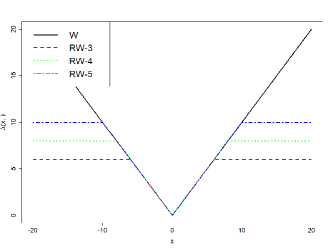
Figure 2: The continuous line represents $\Delta(x,W_{1})$. The dashed (red), dot-dashed (blue) and dotted (green) line represents $\Delta(x,W^{(\lambda)})$ with $\lambda=3,4,5$ respectively.

5.2 Estimation of location

Let us consider problem of inference on univariate location models. We study the robustness of MERWE, comparing its performance to the one of MEWE, under different degrees of data contamination and for different underlying data generating models (with finite and infinite moments). Before delving into the numerical exercise, let us give some numerical details. We recall that the MERWE aims at minimizing the function $\theta\mapsto{\rm{E}}_{m}\left[W^{(\lambda)}\left(\hat{\mu}_{n},\hat{\mu}_{\theta,m}\right)\right].$ With the same notation as in Section 4.1, suppose we generate $k$ replications $Z_{1:m}^{(i)},i=1,\ldots,k,$ independently from a reference model $\mu_{\theta}^{(m)}$, and let $\hat{\mu}_{\theta,m}^{(i)}$ denote the empirical probability measure of $Z_{1:m}^{(i)}$. Then the loss function $L_{\text{MERWE}}=k^{-1}\sum_{i=1}^{k}W^{(\lambda)}\left(\hat{\mu}_{n},\hat{\mu}_{\theta,m}^{(i)}\right)$ is a natural estimator of ${\rm E}_{m}[W^{(\lambda)}\left(\hat{\mu}_{n},\hat{\mu}_{\theta,m}\right)]$, since the former converges almost surely to the latter as $k\rightarrow\infty$. We note that the algorithmic complexity in $m$ is super-linear while the complexity in $k$ is linear: the incremental cost of increasing $k$ is lower than that one of increasing $m$. Moreover, an important aspect for the implementation of our estimator is related to the need for specifying a value of $\lambda$. In the next numerical exercises we set $\lambda=5$: this value yields a good performance (in terms of Mean-Squared Error, MSE) of our estimators across the Monte Carlo settings, which consider different models and different levels of contamination. In Section 6, we describe a selection procedure of $\lambda$.

5.2.1 Finite moments

We consider a reference model which is the sum of log-normal random variables. For a given $L\geq 1$, $\gamma\in\mathbb{R}$ and $\sigma>0$, we have $X=\sum_{l=1}^{L}\exp\left(Z_{l}\right),$ where $Z_{1},\ldots,Z_{L}$ are sampled from $\mathcal{N}\left(\gamma,\sigma^{2}\right)$ independently. Suppose we are interested in estimating the location parameter $\gamma$. We investigate the performance of MERWE and MEWE, under different scenarios: namely, in presence of outliers, for different sample sizes and contamination values. Specifically, we consider the model $X_{i}^{(n)}=\sum_{l=1}^{L}\exp(Z_{i_{l}}^{(n)}),l=1,\ldots,L,i=1,\ldots,n,$ where $Z_{i_{l}}^{(n)}\sim\mathcal{N}(\gamma,\sigma)$ for $i=1,\ldots,n_{1}$ (clean part of the sample) and $Z_{i_{l}}^{(n)}\sim\mathcal{N}(\gamma+\eta,\sigma)$ for $i=n_{1}+1,\ldots,n$ (contaminated part of the sample). Therefore, in each sample, there are $n-n_{1}$ outliers of size $\eta$. In our simulation experiments, we set $L=10$, $\gamma=0$ and $\sigma=1$. To implement the MERWE and MEWE of $\gamma$, we choose $m=1000$, $k=20$ and $\lambda=5$. The bias and MSE, based on $1000$ replications, of the estimators are displayed in Table 1, for various sample sizes $n$, different contamination size $\eta$ and proportion of contamination $\varepsilon$. The table illustrates the superior performance (both in terms of bias and MSE) of the MERWE with respect to the MEWE. In small samples ($n=100$), the MERWE has smaller bias and MSE than the MEWE, in all settings. Similar results are available in moderate and large sample size $(n=200$ and $n=1000$). Interestingly, for $n=1000$, MERWE and MEWE have similar performance when $\varepsilon=0$ (no contamination), whilst the MERWE still has smaller MSE for $\varepsilon>0$. This implies that the MERWE maintains good efficiency with respect to MEWE at the reference model.

SETTINGS	$n=100$				$n=200$				$n=1000$
	BIAS		MSE		BIAS		MSE		BIAS		MSE
	MERWE	MEWE	MERWE	MEWE	MERWE	MEWE	MERWE	MEWE	MERWE	MEWE	MERWE	MEWE
$\varepsilon=0.1,\eta=1$	0.049	0.092	0.003	0.010	0.042	0.093	0.002	0.012	0.037	0.086	0.002	0.008
$\varepsilon=0.1,\eta=4$	0.035	0.090	0.002	0.012	0.029	0.097	0.001	0.016	0.013	0.100	$\approx 0$	0.018
$\varepsilon=0.2,\eta=1$	0.071	0.157	0.008	0.028	0.086	0.178	0.009	0.033	0.081	0.172	0.007	0.031
$\varepsilon=0.2,\eta=4$	0.046	0.204	0.003	0.045	0.035	0.203	0.002	0.043	0.017	0.195	$\approx 0$	0.038
$\varepsilon=0$	0.036	0.034	0.002	0.002	0.022	0.022	0.001	0.001	0.012	0.010	$\approx 0$	$\approx 0$

Table 1: The biases and MSEs of the MERWE and MEWE of $\gamma$ for different $n$, $\varepsilon$ and $\eta$.

5.2.2 Infinite moments

Yatracos (2022) recently illustrates that minimum Wasserstein distance estimators do not perform well for heavy-tailed distributions and suggests to avoid the use of minimum Wasserstein distance inference when the underlying distribution has infinite $p$-th moment, with $p\geq 1$. The theoretical developments of Section 3.1 show that our MERWE does not suffer from the same criticism. In the next MC experiment, we illustrate the good performance of MERWE when the data generating process does not admit finite first moment. We consider the problem of estimating the location parameters for a symmetric $\alpha$-stable distribution; see e.g. Samorodnitsky and Taqqu (2017) for a book-length presentation. A stable distribution is characterized by four parameter $(\alpha,\beta,\gamma,\delta)$: $\alpha$ is the index parameter, $\beta$ is the skewness parameter, $\gamma$ is the scale parameter and $\delta$ is the location parameter. It is worth noting that stable distributions have undefined variance for $\alpha<2$, and undefined mean for $\alpha\leq 1$. We consider three parameters setting: (1) $(\alpha,\beta,\gamma,\delta)=(0.5,0,1,0)$, which represents a heavy-tailed distribution without defined mean; (2) $(\alpha,\beta,\gamma,\delta)=(1,0,1,0)$ which is the standard Cauchy distribution, having undefined moment of order $p\geq 1$; (3) $(\alpha,\beta,\gamma,\delta)=(1.1,0,1,0)$ representing a distribution having a finite mean. In each MC experiment, we estimate the location parameter, while the other parameters are supposed to be known. In addition, we consider contaminated heavy-tailed data, where $1-\varepsilon$ proportion of $n$ observations is generated from $\alpha$-stable distribution with parameter $(\alpha,\beta,\gamma,\delta)$ and the other $\varepsilon$ proportion (outliers) comes from the distribution with parameter $(\alpha,\beta,\gamma,\delta+\eta)$ ($\eta$ is the size of outliers). We set $m=1000$, $n=100$ and $k=20$ and repeat the experiment 1000 times for each distribution and estimator, and $\lambda=5$. We display the results in Table 2. For the stable distributions, the MEWE has larger bias and MSE than the ones yielded by the MERWE. This aspect is particularly evident for the distributions with undefined first moment, namely the Cauchy distribution and the stable distribution with $\alpha=0.5$. These experiments, complementing the ones available in Yatracos (2022), illustrate that while MEWE (which is not well-defined in the considered setting) entails large bias and MSE values, MERWE is well-defined and performs well even for stable distributions with infinite moments.

SETTINGS	Cauchy				Stable ($\alpha=0.5$)				Stable ($\alpha=1.1$)
	BIAS		MSE		BIAS		MSE		BIAS		MSE
	MERWE	MEWE	MERWE	MEWE	MERWE	MEWE	MERWE	MEWE	MERWE	MEWE	MERWE	MEWE
$\varepsilon=0.1,\eta=1$	0.084	1.531	0.011	3.628	0.088	3.179	0.011	13.731	0.090	0.658	0.011	1.030
$\varepsilon=0.1,\eta=4$	0.205	1.529	0.047	3.656	0.164	3.174	0.034	13.706	0.207	0.746	0.048	1.051
$\varepsilon=0.2,\eta=1$	0.181	1.502	0.038	3.602	0.171	3.155	0.037	12.840	0.181	0.676	0.038	0.942
$\varepsilon=0.2,\eta=4$	0.459	1.820	0.224	4.691	0.384	3.140	0.166	12.713	0.485	1.072	0.245	1.802
$\varepsilon=0$	0.046	1.551	0.003	3.740	0.045	3.118	0.003	12.600	0.042	0.613	0.003	0.894

Table 2: The biases and MSEs of the MERWE and MEWE of location parameter for various contaminated $\alpha$-stable distributions. Simulation setting: $m=1000$, $k=20$.

5.3 Generative Adversarial Networks (GAN)

We propose two RWGAN deep learning models: both approaches are based on ROBOT. The first one is derived directly from the dual form in Th. 1, while the second one is derived from (3). We compare these two methods with routinely-applied Wasserstein GAN (WGAN) and with the robust WGAN introduced by Balaji et al. (2020).

5.3.1 Robust GAN: sketch of the methodology

GAN is a deep learning method, first proposed by Goodfellow et al. (2014). It is one of the most popular machine learning approaches for unsupervised learning on complex distributions. GAN includes a generator and a discriminator that are both neural networks and the procedure is based on mutual game learning between them. The generator creates fake samples as well as possible to deceive the discriminator, while the discriminator needs to be more and more powerful to detect the fake samples. The ultimate goal of this procedure is to produce a generator with a great ability to produce high-quality samples just like the original sample.

To illustrate the connections with the ROBOT, let us consider the following GAN architecture; more details are available in the Supplementary Material (Appendix C.2). Let ${X}\sim{\rm P_{r}}$ and ${Z}\sim{\rm P}_{z}$, where $\rm P_{r}$ and ${\rm P}_{z}$ denote the distribution of the reference sample and of a random sample which is the input for the generator. Then, denote by $G_{\theta}$ the function applied by generator (it transforms $Z$ to create fake samples, which are the output of a statistical model ${\rm P}_{\theta}$, indexed by the finite dimensional parameter $\theta$) and by $D_{\vartheta}$ the function applied by the discriminator (it is indexed by a finite dimensional parameter $\vartheta$, which outputs the estimate of the probability that the sample is true). The objective function is

$$\min_{\theta}\max_{\vartheta}\left\{{\rm E}[\log D_{\vartheta}({X})]+{\rm E}[\log(1-D_{\vartheta}(G_{\theta}{(Z)}))]\right\},$$ (14)

where $D_{\vartheta}(X)$ represents the probability that $X$ came from the data rather than $P_{\theta}$. The GAN mechanism trains $D_{\vartheta}$ to maximize the probability of assigning the correct label to both training examples and fake samples. Simultaneously, it trains $G_{\theta}$ to minimize $\log(1-D(G(z)))$. In other words, we would like to train $G_{\theta}$ such that $\mathrm{P_{\theta}}$ is very close (in some distance or divergence) to $\mathrm{P_{r}}$.

Despite its popularity, GAN has some inference issues. For instance, during the training, the generator may collapse to a setting where it always produces the same samples or fast vanishing gradient. Thus, training GANs is a delicate and unstable numerical and inferential task; see Arjovsky et al. (2017). To overcome these problems, Arjovsky et al. propose the so-called Wasserstein GAN (WGAN) based on Wasserstein distance. The main idea is still based on mutual learning, but rather than using a discriminator to predict the probability of generated images as being real or fake, the WGAN replaces $D_{\vartheta}$ with a function $f_{\xi}$ (it corresponds to $\psi$ in Kantorovich-Rubenstein duality), indexed by parameter $\xi$, which is called “a critic”, namely a function that evaluates the realness or fakeness of a given sample. In mathematical form, the WGAN objective function is

$$\min_{\theta}\sup_{\|f_{\xi}\|_{L}\leq 1}\left\{{\rm E}[f_{\xi}({X})]-{\rm E}[f_{\xi}(G_{\theta}({Z}))]\right\},$$ (15)

Also in this new formulation, the task $G_{\theta}$ is still to train $G_{\theta}$ such that $\mathrm{P_{\theta}}$ is very close (now, in Wasserstein distance) to $\mathrm{P_{r}}$. Arjovsky et al. (2017) explain how the WGAN is connected to minimum distance estimation. Following the results in Arjovsky et al., we remark that (15) has the same form as the Kantorovich-Rubenstein duality. Therefore, we apply our dual form of ROBOT in Th. 1 to the WGAN to obtain a new objective function

$$\min_{\theta}\sup_{\|f_{\xi}\|_{L}\leq 1,{\rm range}(f_{\xi})\leq 2\lambda}\left\{{\rm E}[f_{\xi}({X})]-{\rm E}[f_{\xi}(G_{\theta}({Z}))]\right\}.$$ (16)

The central idea is to train a RWGAN by minimizing the robust Wasserstein distance (actually, using the dual form) between real and generative data. To this end, we define a novel RWGAN model based on (16). The algorithm for training this RWGAN model is very similar to the one for WGAN available in Arjovsky et al. (2017), to which we refer for the implementation. We label this robust GAN model as RWGAN-1. Besides this model, we propose another approach derived from (3), where we use a new neural network to represent the modified distribution and add a penalty term to (15) in order to control modification. Because of space constraint, the details of this procedure are provided in Algorithm 2 in Appendix C.2. We label this new RWGAN model as RWGAN-2. Different from Balaji et al. (2020)’s robust GAN, which uses $\chi_{2}$-divergence to constrain the modification of distribution, our RWGAN-2 does this by making use of the TV. In the sequel, we will write RWGAN-B for the robust GAN of Balaji et al. (2020). We remark that the RWGAN-1 is less computationally complex than RWGAN-2 and RWGAN-B. Indeed, RWGAN-2 and RWGAN-B make use of some regularized terms, thus an additional neural network is needed to represent the modification of the distribution. In contrast, RWGAN-1 has a simpler structure: for its implementation, it requires only a small modification of the activation function in the generator network; see Appendix C.2.

5.3.2 Synthetic data

We investigate, via simulated data, the robustness of RWGAN-1 and RWGAN-2. We consider reference samples generated from a simple model, where $n$ points, including $n-n_{1}$ outliers,

$$\begin{array}[]{cc}&X_{i_{1}}^{(n)}\sim\mathrm{U}(0,1),X_{i_{2}}^{(n)}=X_{i_{1}}^{(n)}+1,\\ &{X}_{i}^{(n)}=(X_{i_{1}}^{(n)},X_{i_{2}}^{(n)}),i=1,2,\ldots,n_{1},\\ &{X}_{i}^{(n)}=(X_{i_{1}}^{(n)},X_{i_{2}}^{(n)}+\eta),i=n_{1}+1,n_{1}+2,\ldots,n,\end{array}$$ (17)

with $\eta$ representing the size of outliers. We set $n=1000$ and try four different settings by changing values of $\varepsilon=(n-n_{1})/n$ and $\eta$. As it is common in the GAN literature, our generative adversarial models are obtained using the Python library Pytorch; see Appendix C.2. We display the results in Figure 3, where we compare WGAN, RWGAN-1, RWGAN-2 and RWGAN-B. To measure the distance between the data simulated by the generator and the input data, we report the Wasserstein distance of order 1. The plots reveal that WGAN is greatly affected by outliers. Differently, RWGAN-2 and RWGAN-B are able to generate data roughly consistent with the uncontaminated distribution in most of the settings. Nevertheless, they still produce some obvious abnormal points, especially when the proportion and size of outliers increase. In a very different way, RWGAN-1 performs better than its competitors and generates data that agree with the uncontaminated distribution, even when the proportion and size of outliers are large. Several repetitions of the experiment lead to the same conclusions.

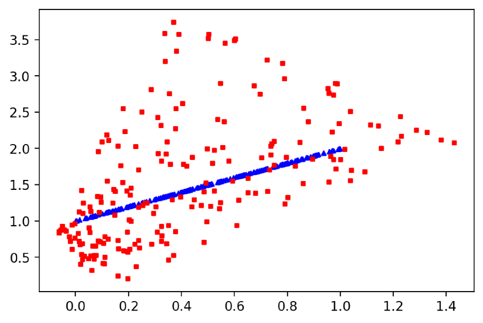
(a) $W^{1}=$ 0.5864

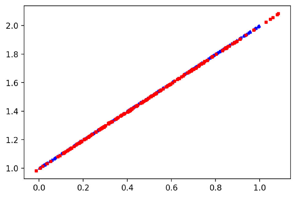
(b) $W^{1}=$ 0.0514

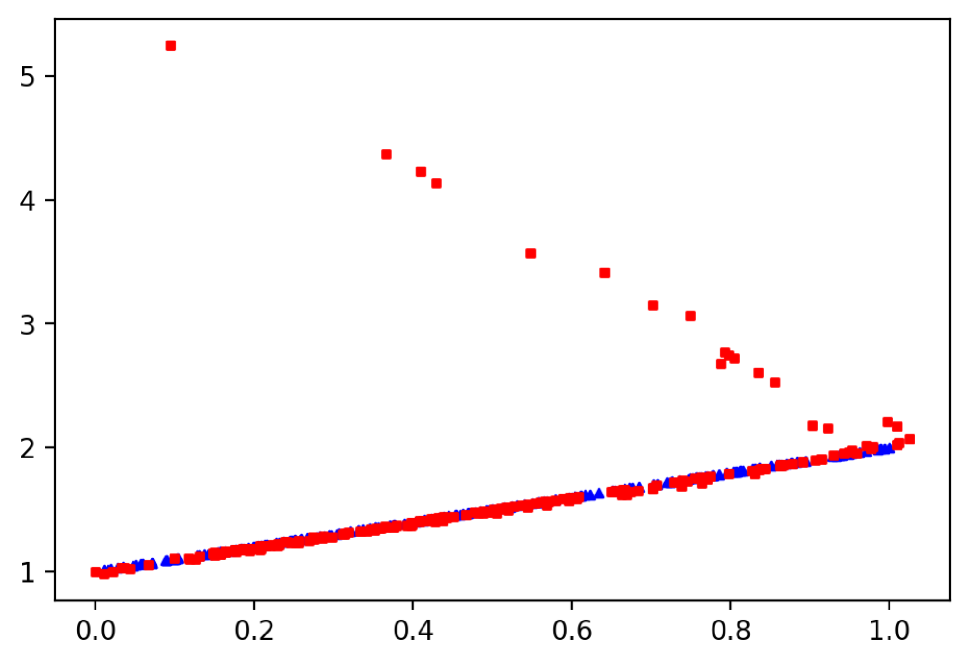
(c) $W^{1}=$ 0.1560

(d) $W^{1}=$ 0.1771

(e) $W^{1}=$ 0.5229

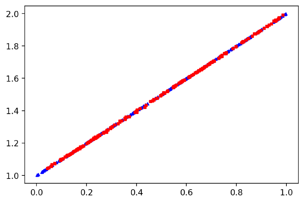
(f) $W^{1}=$ 0.0495

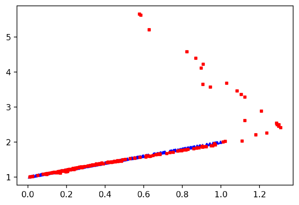
(g) $W^{1}=$ 0.2312

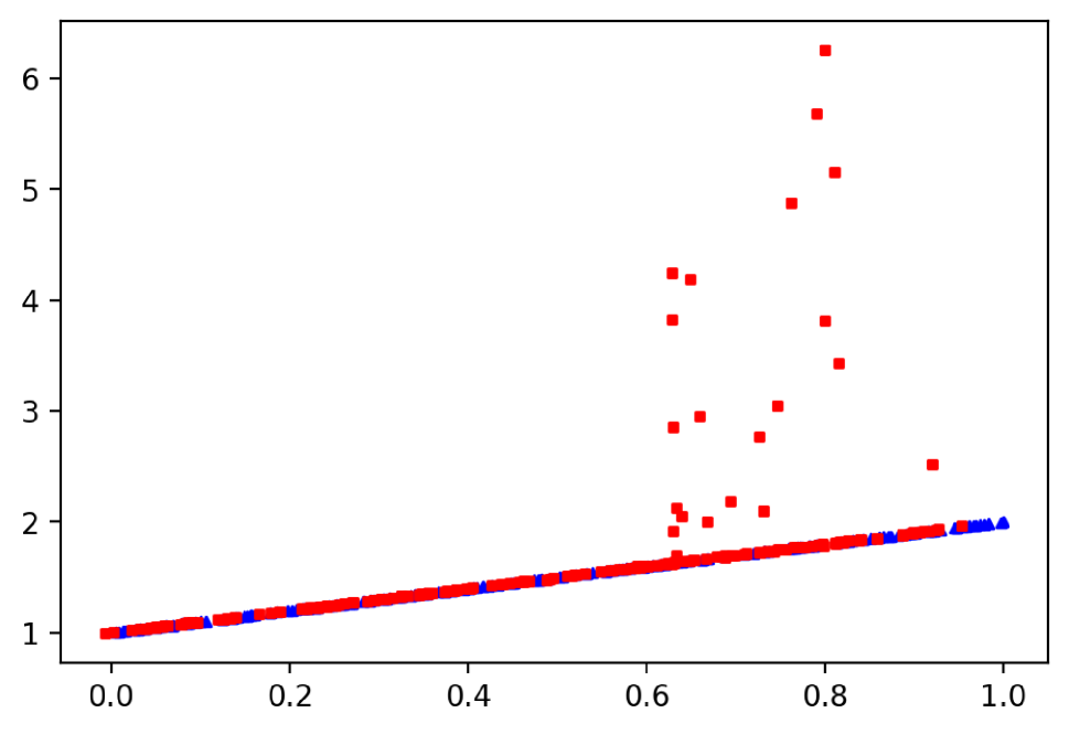
(h) $W^{1}=$ 0.1803

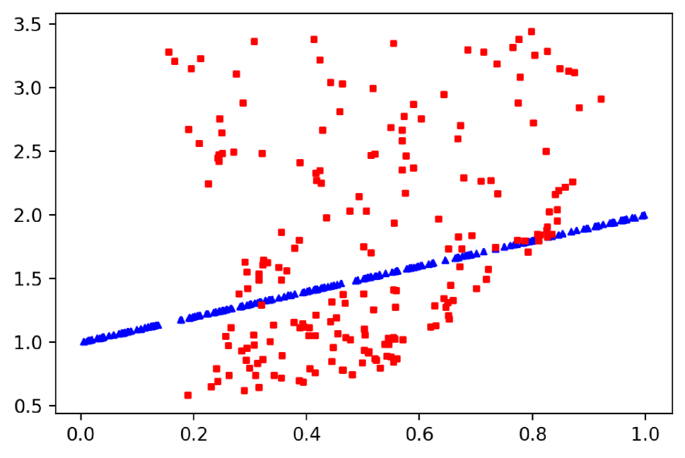
(i) $W^{1}=$ 0.5646

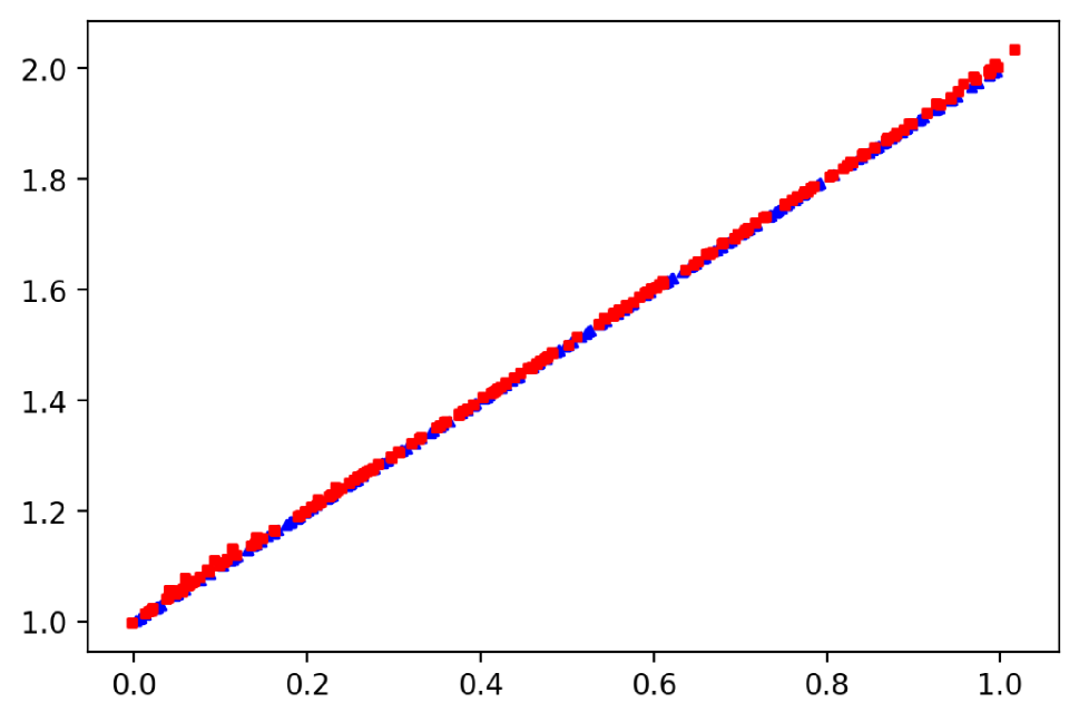
(j) $W^{1}=$ 0.0470

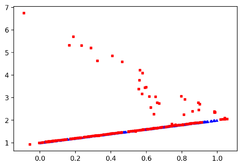
(k) $W^{1}=$ 0.2938

(l) $W^{1}=$ 0.3229

(m) $W^{1}=$ 0.6518

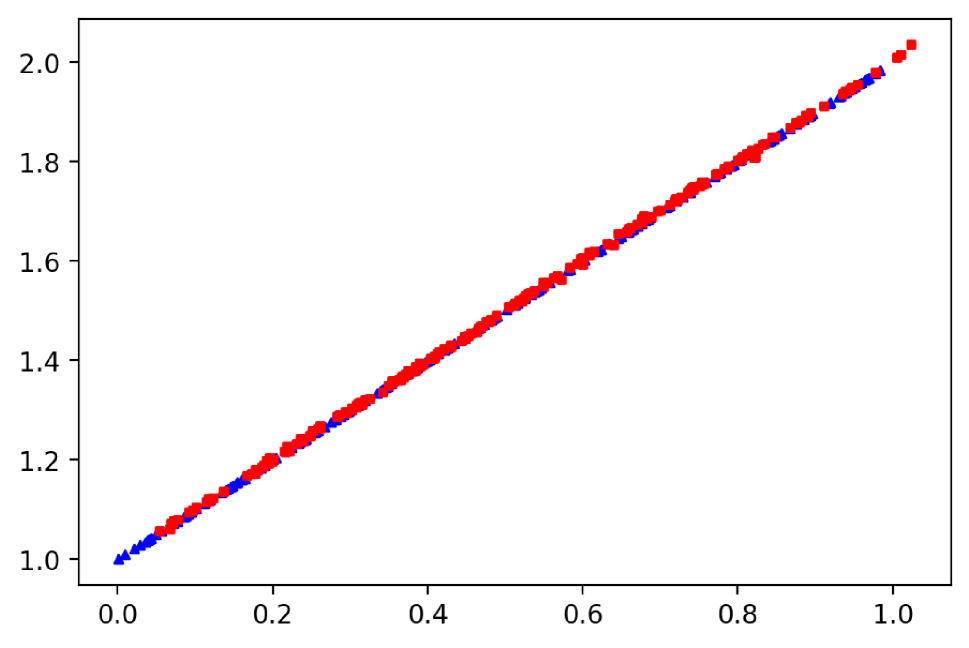
(n) $W^{1}=$ 0.0471

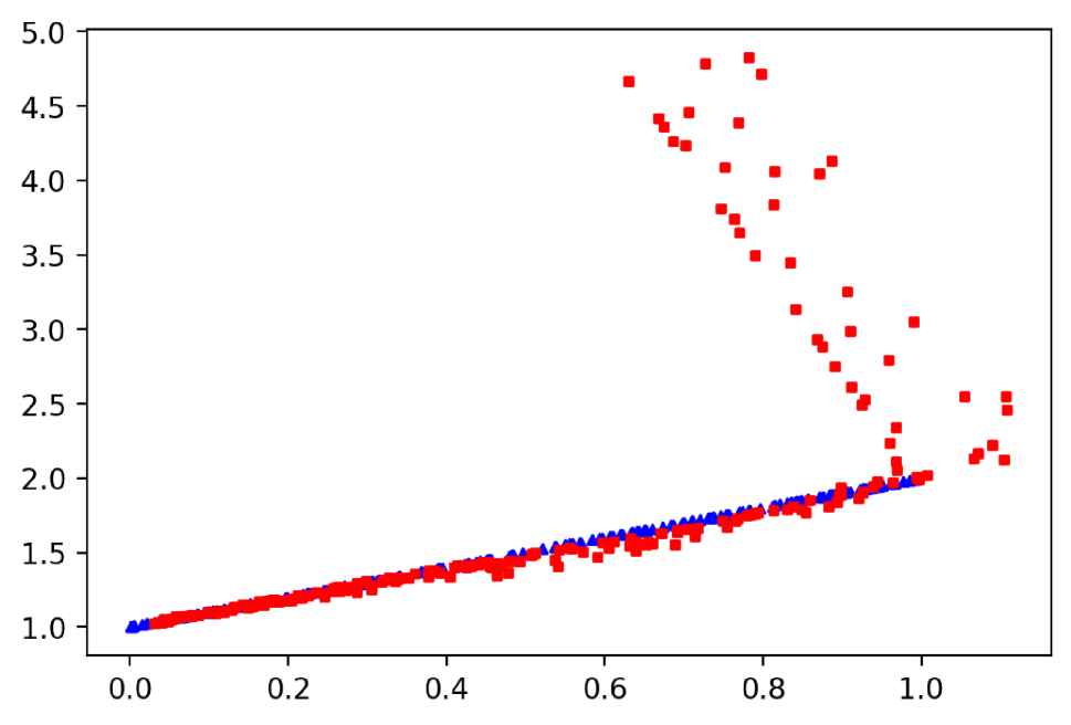
(o) $W^{1}=$ 0.3954

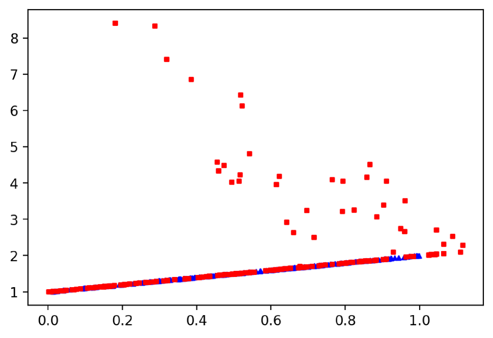
(p) $W^{1}=$ 0.4674

Figure 3: Blue triangles: 200 data points sampled from the reference distribution (uncontaminated observations). Red squares: 200 data points generated from WGAN (1st column), RWGAN-1 (2nd column), RWGAN-2 (3rd column) and RWGAN-B (4th column). Empirical Wasserstein distance $p=1$ between triangles and squares is provided. (1st row: $\varepsilon=0.1$,$\eta=2$; 2nd row: $\varepsilon=0.1$,$\eta=3$; 3rd row: $\varepsilon=0.2$,$\eta=2$; 4th row: $\varepsilon=0.2$,$\eta=3$).

5.3.3 Fashion-MNIST real data example

We illustrate the performance of the RWGAN-1 and RWGAN-2 through comparing them with the WGAN and RWGAN-B in analysing the Fashion-MNIST dataset, which contains 70000 grayscale images of apparels, including T-shirt, jeans, pullover, skirt, coat, etc. Each image is of $28\times 28$ pixels, and each pixel gets value from 0 to 255, indicating the darkness or lightness. We generate outlying images by taking the negative effect of images already available in the dataset—a negative image is a total inversion, in which light areas appear dark and vice versa; in the Fashion-MNIST dataset, for each pixel of a negative image, it takes 255 minus the value of the pixel corresponding to the normal picture. By varying the number of negative images we define different levels of contamination: we consider 0, 3000, and 6000 outlying images. For the sake of visualization, in Figure 4(a) and 4(b) we show normal and negative images, respectively. Our goal is to obtain a generator which can produce images of the same style as Figure 4(a), even if it is trained on sample containing normal images and outliers. A more detailed explanation on how images generation works via Pythorc is available in Appendix C.2. In Figure 5, we display images generated by the WGAN, RWGAN-1, RWGAN-2 and RWGAN-B under the different levels of contamination—we select $\lambda$ making use of the data driven procedure described in Section 6. We see that all of the GANs generate similar images when there are no outliers in the reference sample (1st row). When there are 3000 outliers in the reference sample (2nd row), the GANs generate some negative images. However, by a simple eyeball search on the plots, we notice that WGAN produces many obvious negative images, while RWGAN-B, RWGAN-1 and RWGAN-2 generate less outlying images than WGAN. Remarkably, RWGAN-1 produces the smaller number of negative images among the considered methods. Similar conclusions holds for the higher contamination level with 6000 outlying images.

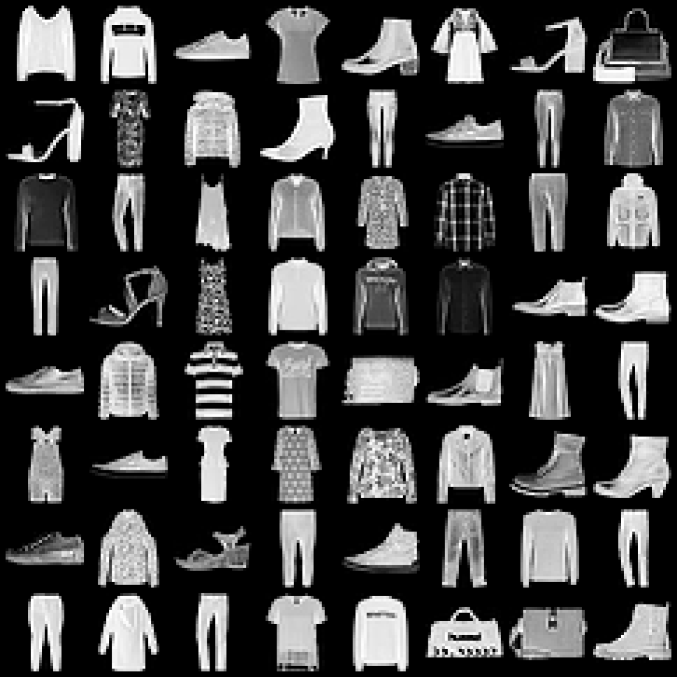
(a) normal image

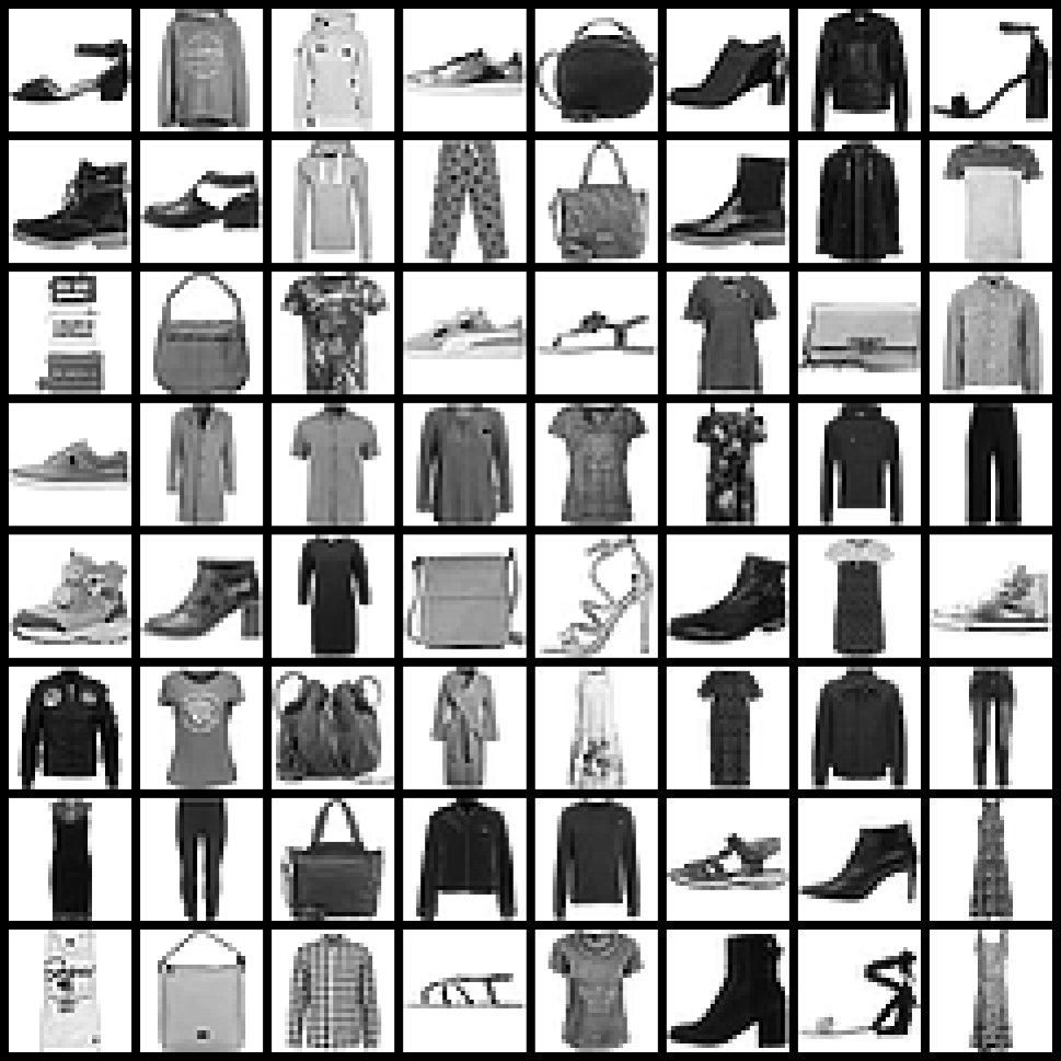
(b) outlying image

Figure 4: Style of clean reference sample images and outlier images. Panel (a) contains pictures that are regarded as the right style. Panel (b) contains negative pictures (outliers).

To quantify the accuracy of these GANs, we train a convolutional neural network (CNN) to classify normal images and negative images, using a training set of 60000 normal images and 60000 negative images. The resulting CNN is 100% accurate on a test set of size 20000. Then, we use this CNN to classify 1000 images generated by the four GANs. In Table 3, we report the frequencies of normal images detected by the CNN. The results are consistent with the eyeball analysis of Figure 5: the RWGAN-1 produces the smaller numbers of negative images at different contamination levels.

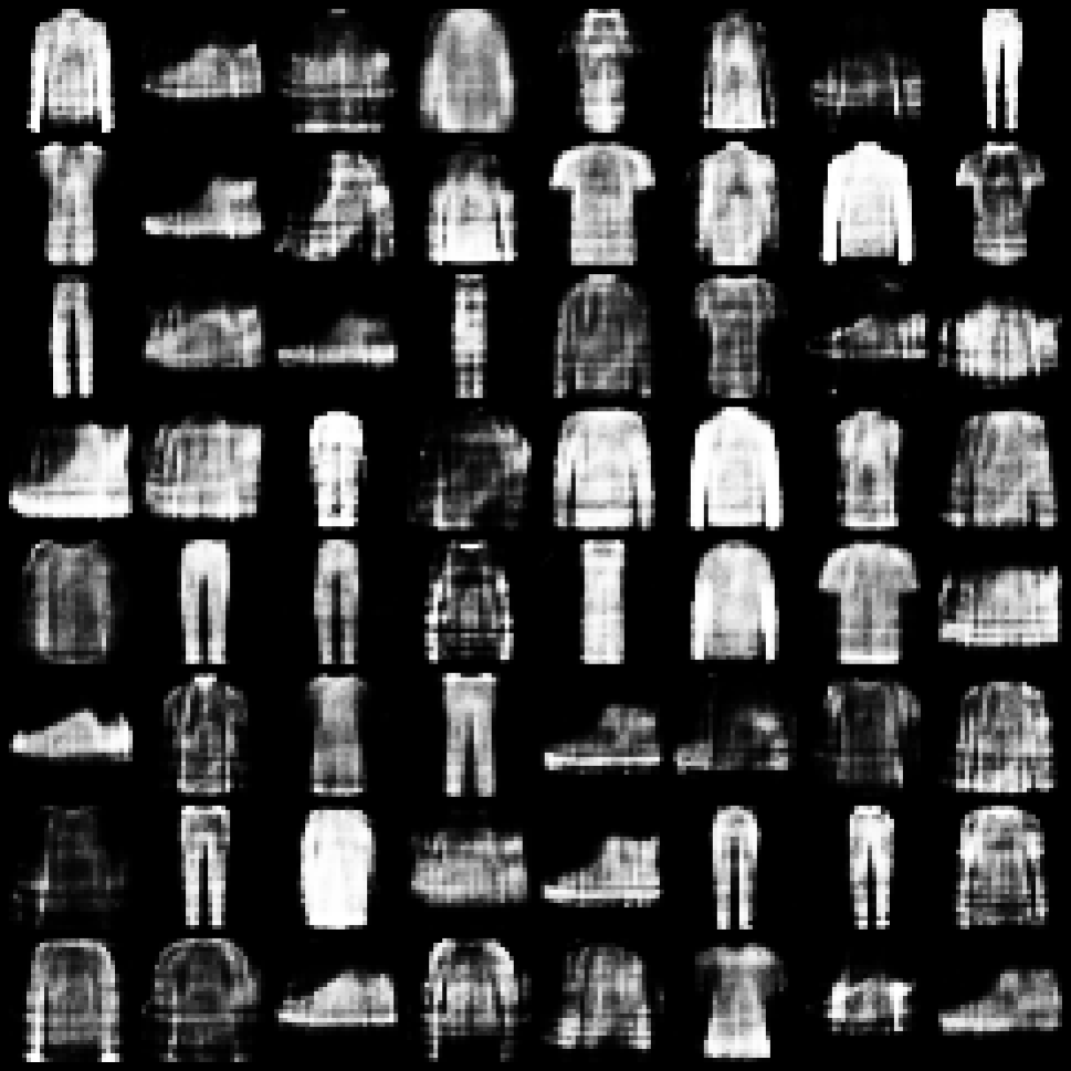
(a)

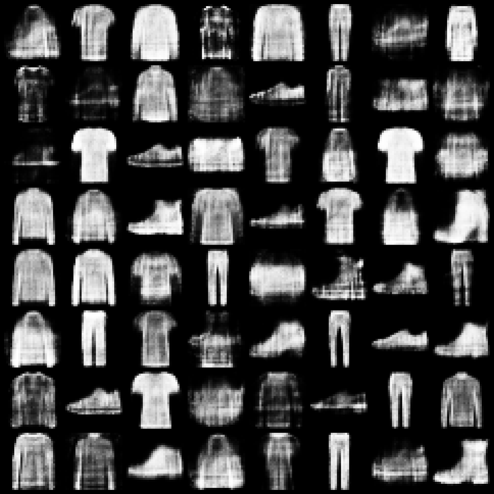
(b)

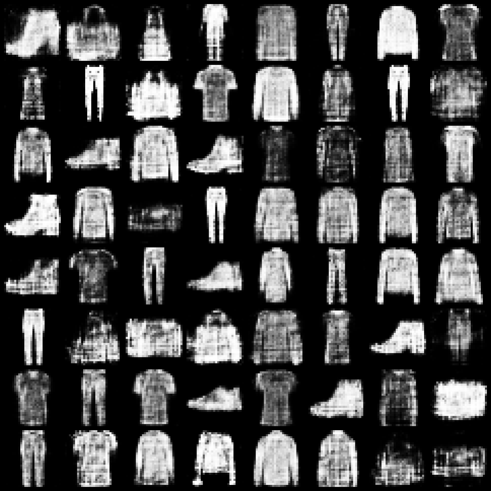
(c)

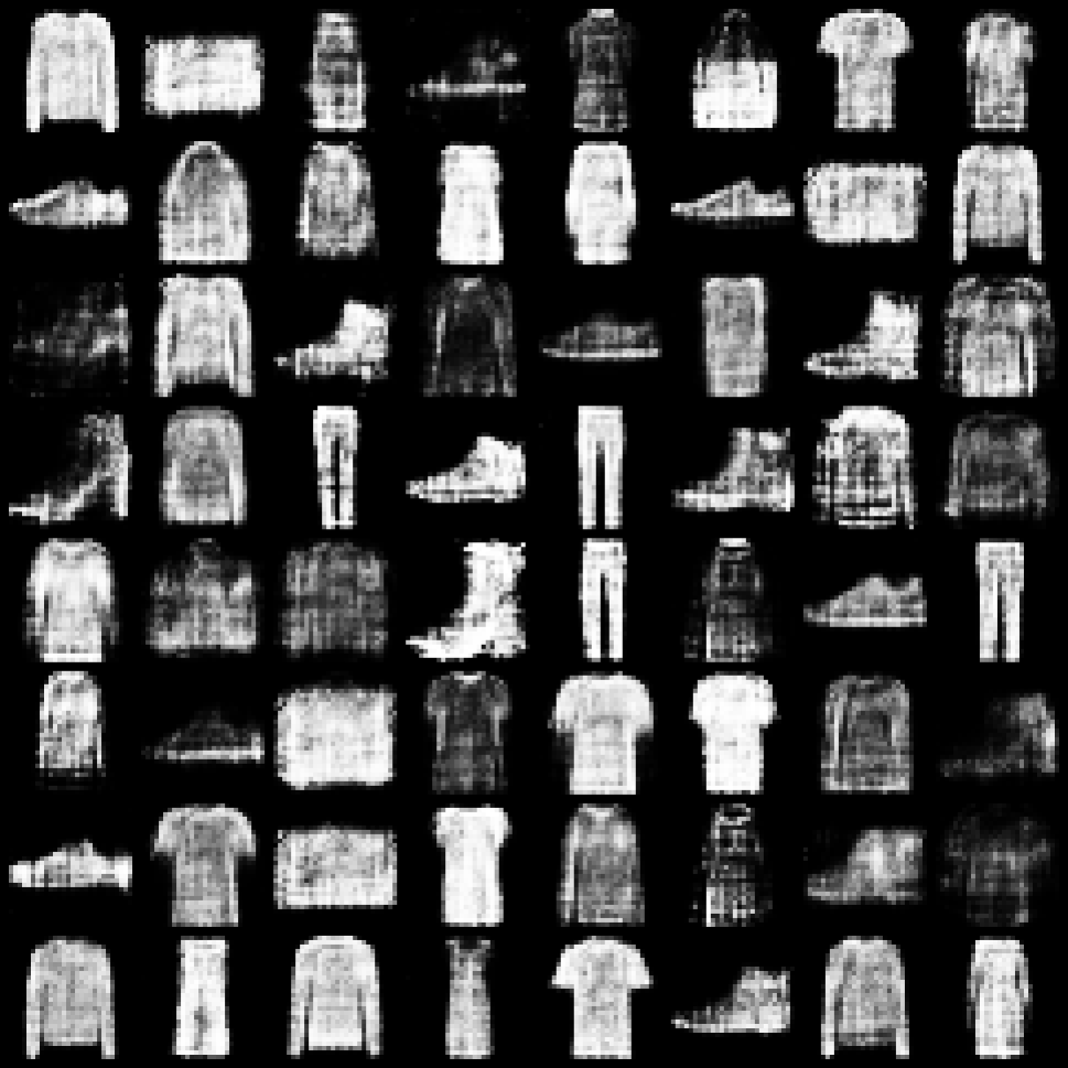
(d)

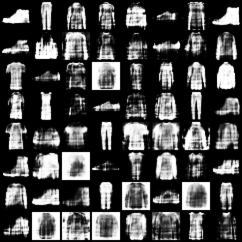
(e)

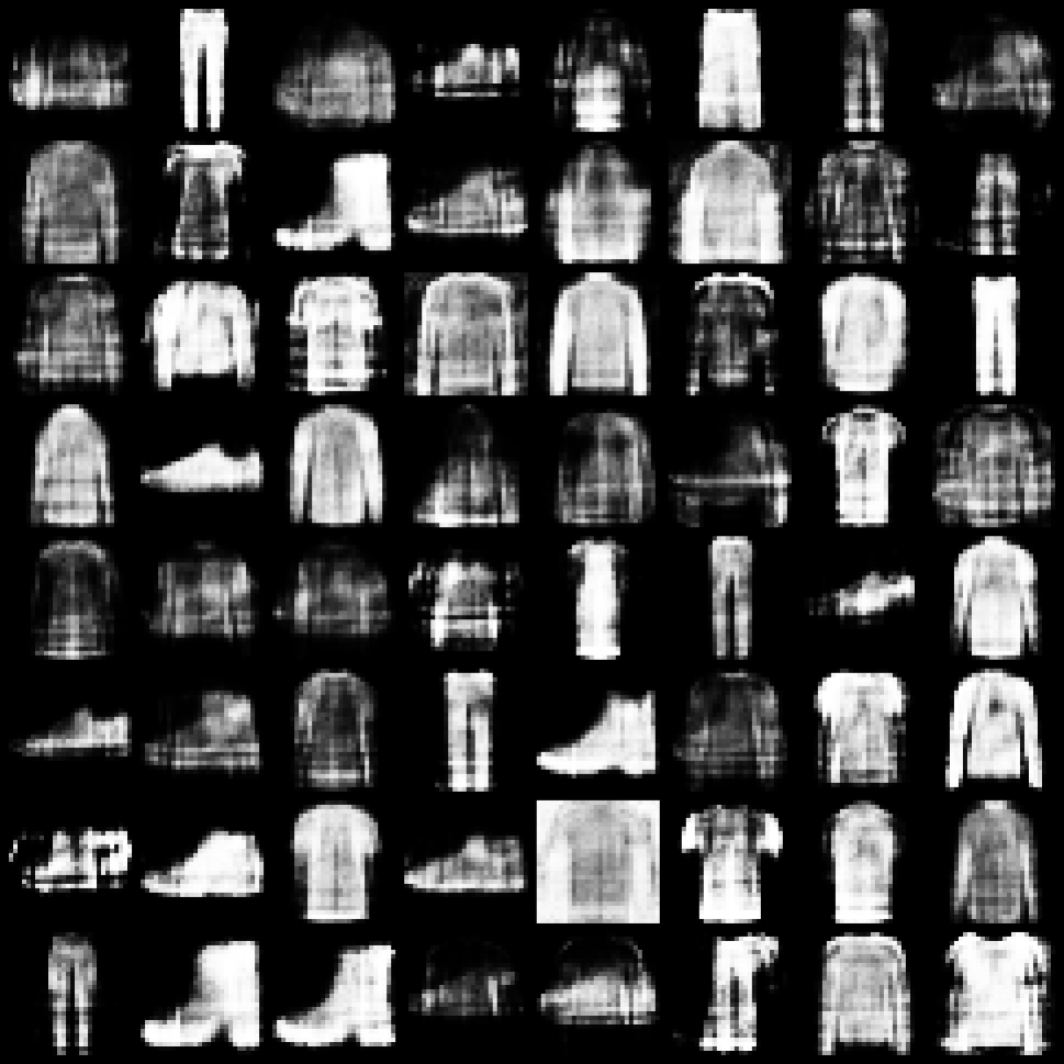
(f)

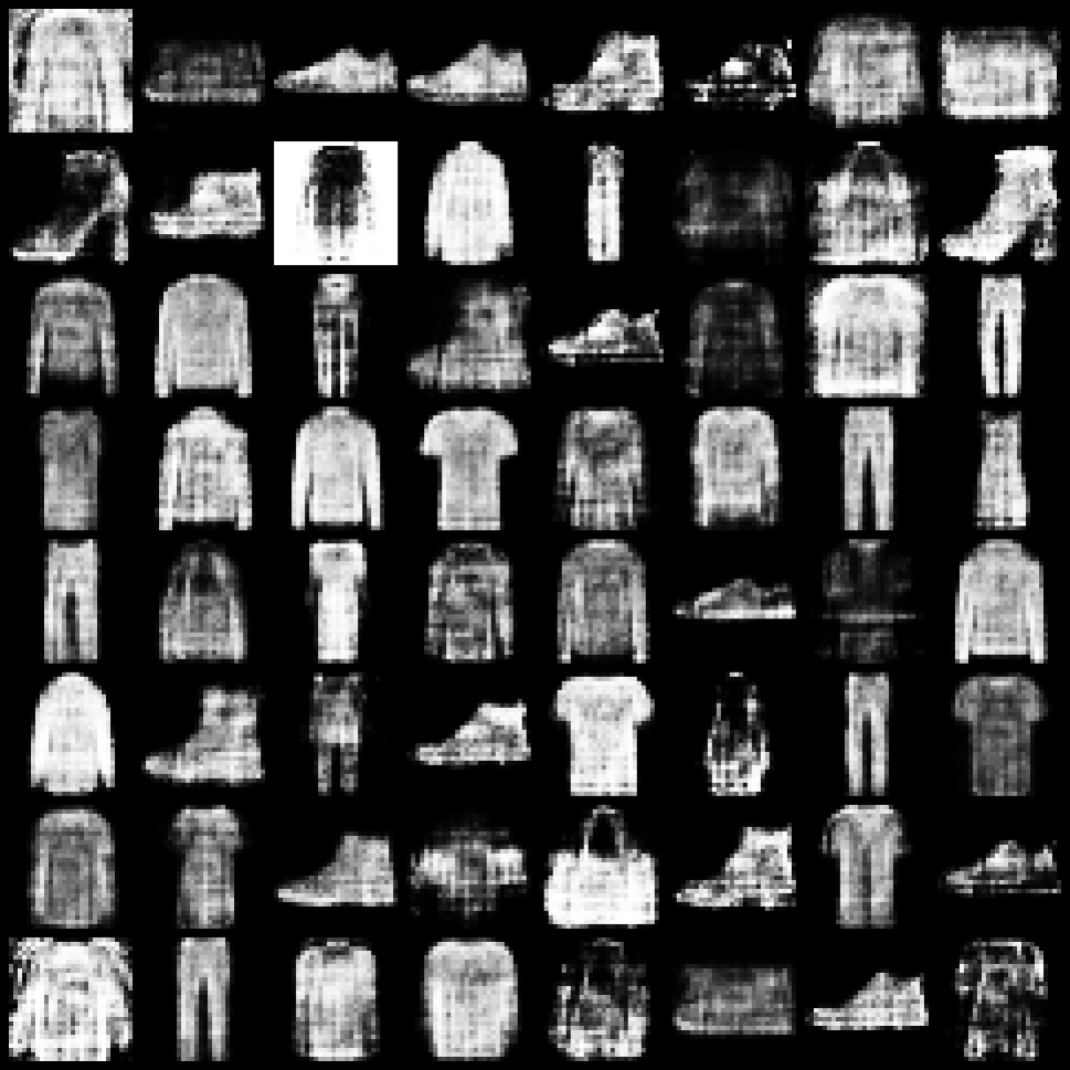
(g)

(h)

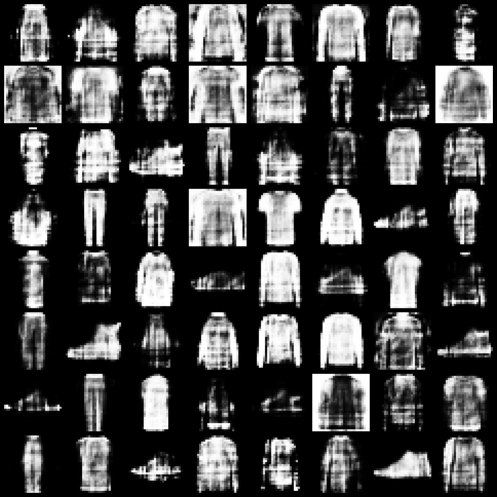
(i)

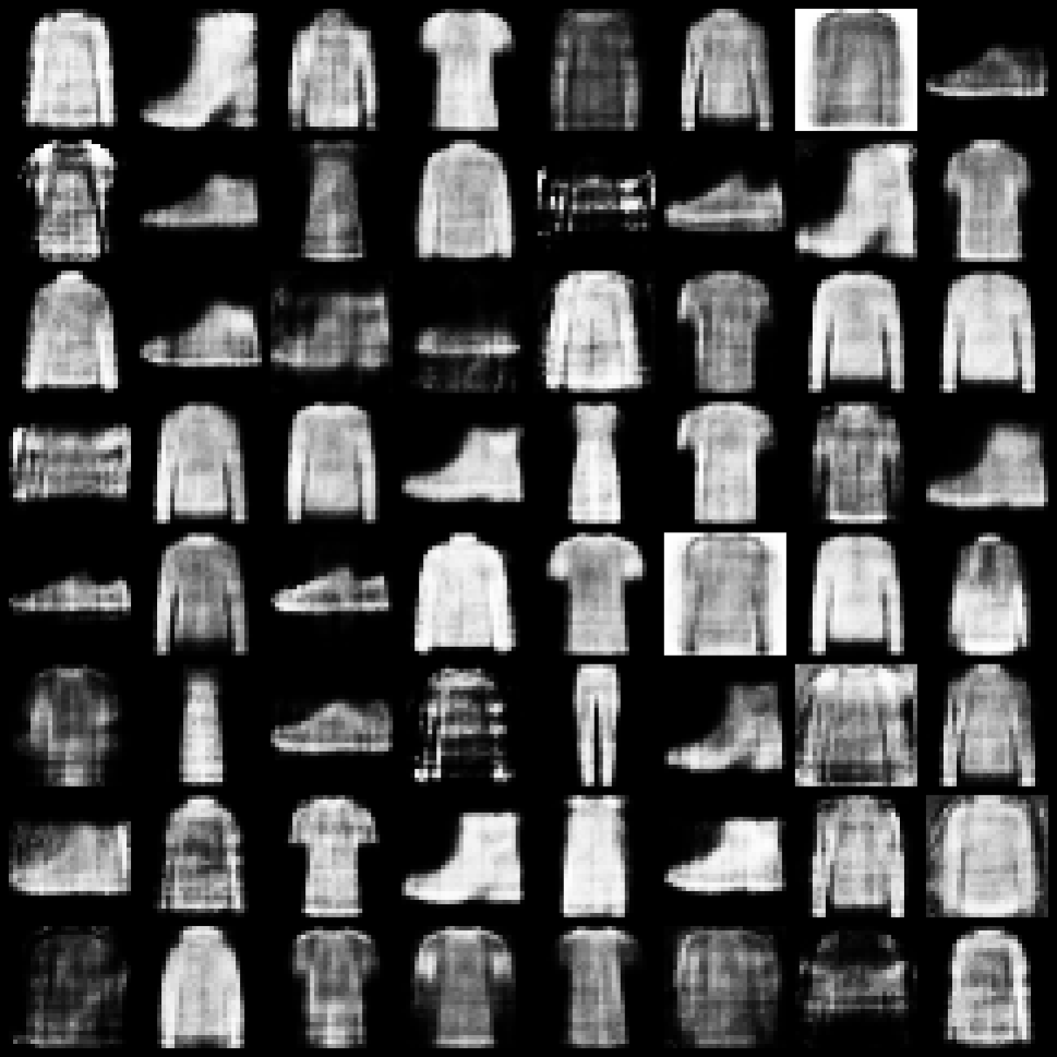
(j)

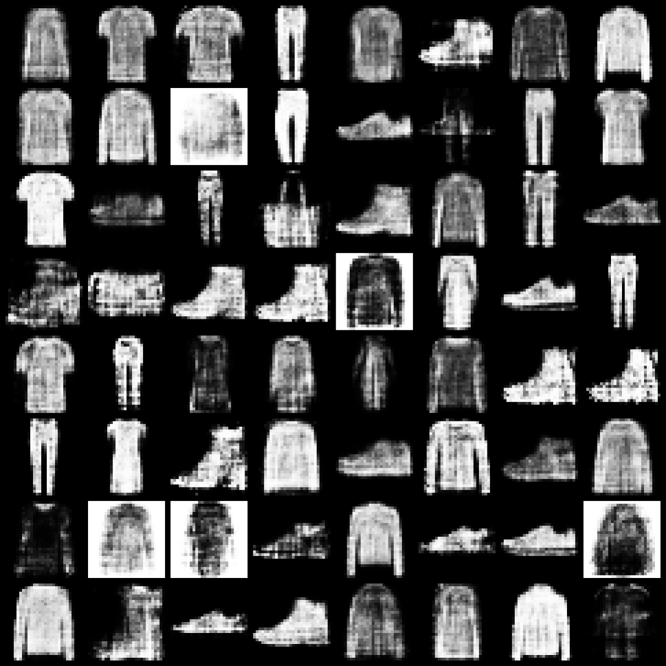
(k)

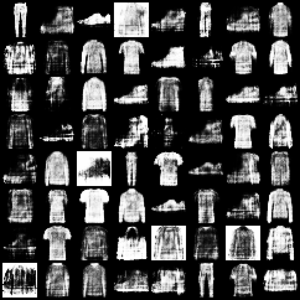
(l)

Figure 5: 64 images generated from WGAN (1st column), RWGAN-1 (2nd column), RWGAN-2 (3rd column) and RWGAN-B (4th column). (1st row: no outliers; 2nd row: 3000 outliers; 3rd row: 6000 outliers).

	WGAN	RWGAN-1	RWGAN-2	RWGAN-B
0 outliers	1.000	1.000	1.000	1.000
3000 outliers	0.941	0.982	0.953	0.945
6000 outliers	0.890	0.975	0.913	0.897

Table 3: Frequency of normal images output for each GAN model, under different contamination levels (the results are based on the classification by a trained CNN model).

6 Choice of $\lambda$ via concentration inequalities

The application of $W^{(\lambda)}$ requires the specification of $\lambda$. In the literature of robust statistics, many selection criteria are based on first-order asymptotic theory: for instance, Mancini et al. (2005) and La Vecchia et al. (2012) propose to select the tuning constant for Huber-type M-estimators achieving a given asymptotic efficiency at the reference model (namely, without considering the contamination). Unfortunately, these type of criteria hinge on the asymptotic notion of influence function, which is not available for our estimators defined in Section 4; see Bassetti and Regazzini (2006) for a related discussion on MKE. Mukherjee et al. (2021) propose a criterion which needs access to a clean data set and do not develop its theoretical underpinning. To fill this gap in the literature, we introduce a selection criterion of $\lambda$ that does not have an asymptotic nature and is data-driven. Moreover, it does not need the computation of $\hat{\theta}^{\lambda}_{n}$ for each $\lambda$, that makes its implementation fast.

To start with, let us call $\theta^{*}\in\arg\min_{\theta}W^{(\lambda)}(\mu_{\theta},\mu_{\star})$. Repeated applications of the triangle inequality yield

$$W^{(\lambda)}(\mu_{\hat{\theta}^{\lambda}_{n}},\mu_{\star}) \leq W^{(\lambda)}(\mu_{\hat{\theta}^{\lambda}_{n}},\hat{\mu}_{n})+W^{(\lambda)}(\hat{\mu}_{n},\mu_{\star})\leq W^{(\lambda)}(\mu_{\theta^{*}},\mu_{\star})+2W^{(\lambda)}(\hat{\mu}_{n},\mu_{\star})$$

$$\leq W^{(\lambda)}(\mu_{\theta^{*}},\mu_{\star})+2{\rm E}[W^{(\lambda)}(\hat{\mu}_{n},\mu_{\star})]+2|W^{(\lambda)}(\hat{\mu}_{n},\mu_{\star})-{\rm E}[W^{(\lambda)}(\hat{\mu}_{n},\mu_{\star})]|,$$

which suggests that $|W^{(\lambda)}(\hat{\mu}_{n},\mu_{\star})-{\rm E}[W^{(\lambda)}(\hat{\mu}_{n},\mu_{\star})]|$ has an influence on the behavior of $W^{(\lambda)}(\mu_{\hat{\theta}},\mu_{\star})$. Heuristically, small values of $\left|W^{(\lambda)}(\hat{\mu}_{n},\mu_{\star})-{\rm E}[W^{(\lambda)}(\hat{\mu}_{n},\mu_{\star})]\right|$ yield a control on the robust Wasserstein distance between the fitted model $\mu_{\hat{\theta}}$ and the actual data generating measure $\mu_{\star}$. This consideration suggests that to control the behavior of $\hat{\theta}^{\lambda}_{n}$ we need to focus on the concentration of $W^{(\lambda)}(\hat{\mu}_{n},\mu)$ about its mean. To study this quantity, we make use of (9) and (10): we define a data driven (i.e. depending on $n$, on the estimated $\sigma$ and on the guessed $|O|$) selection criterion for $\lambda$. The central idea hinges on the fact that $\lambda$ controls the impact that the outliers have on the concentration bounds. Given a user-specified value for the percentage of outliers (this value does not necessarily needs to coincide with the actual percentage of contaminated data, see Appendix D.2), the resulting criterion allows to identify a range of sensible values of $\lambda$, which are not too close to zero and not too large either. This is a suitable and sensible achievement. Indeed, on the one hand, values of $\lambda$ too close to zero imply that $W^{(\lambda)}$ trims too many observations which likely include inliers and most outliers. On the other hand too large values of $\lambda$ imply that $W^{(\lambda)}$ trims a very limited number of outliers; see Appendix D.1 for a numerical illustration of this aspect in terms of MSE as a function of $\lambda$. Due to space constraints, the methodological aspects of the selection procedure and its numerical illustration are deferred to Appendix D.2. In Appendix D.1, we make use of RWGAN to provide some considerations on the role of $\lambda$.

SUPPLEMENTARY MATERIAL

Appendix A provides some key theoretical results of optimal transport. All proofs are collected in Appendix B. Appendix C, as a complement to Section 5, provides more details and additional numerical results of a few applications of ROBOT—see Appendix C.1 for an application of ROBOT to detect outliers in the context of parametric estimation in a linear regression model. Appendix D contains the methodological aspects of $\lambda$ selection. In Appendix E, we consider an application of ROBOT to domain adaptation.

Appendix A Some key theoretical details about optimal transport

This section is a supplementary to Section 2.1. For deep details about optimal transport, we refer the reader to Villani (2003, 2009).

Measure transportation theory dates back to the celebrated work Monge (1781), in which Monge formulated a mathematical problem that in modern language can be expressed as follows. Given two probability measures $\mu\in\mathcal{P(X)}$, $\nu\in\mathcal{P(Y)}$ and a cost function $c:\mathcal{X\times Y}\rightarrow[0,+\infty]$, Monge’s problem is to solve the minimization equation

$$\inf\left\{{\int_{\mathcal{X}}c(x,\mathcal{T}(x))d\mu(x):\mathcal{T}\#\mu=\nu}\right\}$$ (18)

(in the measure transportation terminology, $\mathcal{T}\#\mu=\nu$ means that $\mathcal{T}$ is pushing $\mu$ foward to $\nu$). The solution to the Monge’s problem (MP) (18) is called optimal transport map. Informally, one says that $\mathcal{T}$ transports the mass represented by the measure $\mu$ to the mass represented by the measure $\nu$. The optimal transport map which solves problem (18) (for a given $c$) hence naturally yields minimal cost of transportation.

It should be stressed that Monge’s formulation has two undesirable prospectives. First, for some measures, no solution to (18) exists. Considering, for instance, the case that $\mu$ is a Dirac measure while $\nu$ is not, there is no transport map which transport mass between $\mu$ and $\nu$. Second, since the set $\{\mu,{\cal T}(\nu)\}$ of all measurable transport map is non-convex, solving problem (18) is algorithmically challenging.

Monge’s problem was revisited by Kantorovich (1942), in which a more flexible and computationally feasible formulation was proposed. The intuition behind the the Kantorovich’s problem is that mass can be disassembled and combined freely. Let $\Pi(\mu,\nu)$ denote the set of all joint probability measures of $\mu\in\mathcal{P(X)}$ and $\nu\in\mathcal{P(Y)}$. Kontorovich’s problem aims at finding a joint distribution $\pi\in\Pi(\mu,\nu)$ which minimizes the expectation of the coupling between $X$ and $Y$ in terms of the cost function $c$, and it can be formulated as

$$\inf\left\{\int_{\mathcal{X\times Y}}c(x,y)d\pi(x,y):\pi\in\Pi(\mu,\nu)\right\}.$$ (19)

A solution to Kantorovich’s problem (KP) (19) is called an optimal transport plan. Note that Kantorovich’s problem is more general than Monge’s one, since it allows for mass splitting. Moreover, unlike $\{\mu,{\cal T}(\nu)\}$, the set $\Pi(\mu,\nu)$ is convex, and the solution to (19) exists under some mild assumptions on $c$, e.g., lower semicontinuous (see Villani (2009, Chapter 4)). Brenier (1987) established the relationship between optimal transport plan and optimal transport map when the cost function is the squared Euclidean distance. More specifically, the optimal transport plan $\pi$ can be expressed as $(\mathrm{Id},\mathcal{T})_{\#}\mu$.

The dual form (KD) of Kantorovich’s primal minimization problem (19) is to solve the maximization problem

$$\begin{array}[]{ll}&\sup\left\{\int_{\mathcal{Y}}\phi d\nu-\int_{\mathcal{X}}\psi d\mu:\phi\in C_{b}(\mathcal{Y}),\psi\in C_{b}(\mathcal{X})\right\}\\ &{\rm s.t.}\quad\phi(y)-\psi(x)\leq c(x,y),\enspace\forall(x,y),\end{array}$$ (20)

where $C_{b}(\mathcal{X})$ is the set of bounded continuous functions on $\mathcal{X}$. According to Theorem 5.10 in Villani (2009), if the cost function $c$ is a lower semicontinuous, there exists a solution to the dual problem such that the solutions to KD and KP coincide, namely there is no duality gap. In this case, the solution takes the form

$$\phi(y)=\inf\limits_{x\in\mathcal{X}}[\psi(x)+c(x,y)]\quad\text{and}\quad\psi(x)=\sup\limits_{y\in\mathcal{Y}}[\phi(y)-c(x,y)],$$ (21)

where the functions $\phi$ and $\psi$ are called $c$-concave and $c$-convex, respectively, and $\phi$ (resp. $\psi$) is called the $c$-transform of $\psi$ (resp. $\phi$). A special case is that when $c$ is a metric on $\mathcal{X}$, equation (20) simplifies to

$$\sup\left\{\int_{\mathcal{Y}}\psi d\nu-\int_{\mathcal{X}}\psi d\mu:\psi\,\text{is 1-Lipschitz continuous}\right\},$$ (22)

This case is commonly known as Kantorovich-Rubenstein duality.

Another important concept in measure transportation theory is Wasserstein distance. Let $(\mathcal{X},d)$ denote a complete metric space equipped with a metric $d:\mathcal{X}\times\mathcal{X}\rightarrow\mathbb{R}$, and let $\mu$ and $\nu$ be two probability measures on $\mathcal{X}$. Solving the optimal transport problem in (19), with the cost function $c(x,y)=d^{p}(x,y)$, would introduce a distance, called Wasserstein distance, between $\mu$ and $\nu$. More specifically, the Wasserstein distance of order $p$ $(p\geq 1)$ is defined by (2).

Appendix B Proofs

Proof of Theorem 1. First, if $\psi(y)-\psi(x)\leq c(x,y)$, then $\psi(y)-c(x,y)\leq\psi(x)$ and hence

$$\sup\limits_{y\in\mathcal{X}}(\psi(y)-c(x,y))\leq\psi(x),$$

where the supremum of the left-hand side is reached when $y=x$. Therefore, $\psi(x)$ is c-convex and $\psi(x)=\psi^{c}(x)$.

Combined with Theorem 5.10 in Villani (2009), the proof can be completed. ∎

Proof of Lemma 1. We will prove that $c_{\lambda}$ satisfies the axioms of a distance. Let $x,y,z$ be three points in the space $\mathcal{X}$. First, the symmetry of $c_{\lambda}(x,y)$, that is, $c_{\lambda}(x,y)=c_{\lambda}(y,x)$, follows immediately from $\min\{c(x,y),2\lambda\}=\min\{c(y,x),2\lambda\}$.

Next, it is obvious that $c_{\lambda}(x,x)=0$. Assuming that $c_{\lambda}(x,y)=0$, then

$$\min\{c(x,y),2\lambda\}=c(x,y)=0,$$

which entails that $x=y$ since $c(x,y)$ is a metric. By definition, we also have $c_{\lambda}(x,y)\geq 0$ for all $x,y\in\mathcal{X}$.

Finally, note that

$$c_{\lambda}(x,z)+c_{\lambda}(y,z)>2\lambda\geq\min\{c(x,y),2\lambda\}=c_{\lambda}(x,y)$$

when $c(x,z)$ or $c(y,z)>2\lambda$, and

$$c_{\lambda}(x,z)+c_{\lambda}(y,z)=c(x,z)+c(y,z)\geq c(x,y)\geq c_{\lambda}(x,y)$$

when $c(x,z)\leq 2\lambda$ and $c(y,z)\leq 2\lambda$.

In summary, $c_{\lambda}$ is a metric on $\mathcal{X}$. ∎

Proof of Theorem 2. We prove that $W^{(\lambda)}$ satisfies the axioms of a distance. First, $W^{(\lambda)}(\mu,\nu)\geq 0$ is obvious. Conversely, letting $\mu,\nu$ be two probability measures such that $W^{(\lambda)}(\mu,\nu)=0$, then there exists at least an optimal transport plan $\pi$ (Villani, 2003). It is clear that the support set of $\pi$ is the diagonal $(y=x)$. Thus, for all continuous and bounded functions $\psi$,

$$\int\psi d\mu=\int\psi(x)d\pi(x,y)=\int\psi(y)d\pi(x,y)=\int\psi d\nu,$$

which implies $\mu=\nu$.

Next, let $\mu_{1},\mu_{2}$ and $\mu_{3}$ be three probability measures on $\mathcal{X}$, and let $\pi_{12}\in\Pi(\mu_{1},\mu_{2})$, $\pi_{23}\in\Pi(\mu_{2},\mu_{3})$ be optimal transport plans. By the Gluing Lemma (Villani, 2003), there exist a probability measure $\pi$ in $\mathcal{P}(\mathcal{X}\times\mathcal{X}\times\mathcal{X})$ with marginals $\pi_{12}$, $\pi_{23}$ and $\pi_{13}$ on $\mathcal{X}\times\mathcal{X}$. Use the triangle inequality in Lemma 1, we obtain

$$W^{(\lambda)}(\mu_{1},\mu_{3}) \leq\int_{\mathcal{X}\times\mathcal{X}}c_{\lambda}(x_{1},x_{3})d\pi_{13}(x_{1},x_{3})$$

$$=\int_{\mathcal{X}\times\mathcal{X}\times\mathcal{X}}c_{\lambda}(x_{1},x_{3})d\pi(x_{1},x_{2},x_{3})$$

$$\leq\int_{\mathcal{X}\times\mathcal{X}\times\mathcal{X}}[c_{\lambda}(x_{1},x_{2})+c_{\lambda}(x_{2},x_{3})]d\pi(x_{1},x_{2},x_{3})$$

$$=\int_{\mathcal{X}\times\mathcal{X}}c_{\lambda}(x_{1},x_{2})d\pi_{12}(x_{1},x_{2})+\int_{\mathcal{X}\times\mathcal{X}}c_{\lambda}(x_{2},x_{3})d\pi_{13}(x_{2},x_{3})$$

$$=W^{(\lambda)}(\mu_{1},\mu_{2})+W^{(\lambda)}(\mu_{2},\mu_{3})$$

Moreover, the symmetry is obvious since $W^{(\lambda)}(\mu,\nu)=\inf\limits_{\pi\in\Pi(\mu,\nu)}\left(\int c_{\lambda}(x,y)d\pi(x,y)\right)=W^{(\lambda)}(\nu,\mu)$.

Finally, note that $W^{(\lambda)}$ is finite since

$$W^{(\lambda)}(\mu,\nu)=\inf\limits_{\pi\in\Pi(\mu,\nu)}\int c_{\lambda}(x,y)d\pi(x,y)\leq\inf\limits_{\pi\in\Pi(\mu,\nu)}\int 2\lambda d\pi(x,y)\leq+\infty.$$

In conclusion, $W^{(\lambda)}$ is a finite distance on $\mathcal{P(X)}$. ∎

Proof of Theorem 3. First, we prove that $W^{(\lambda)}$ is monotonically increasing with respect to $\lambda$. Assuming that $\lambda_{2}>\lambda_{1}>0$, then $c_{\lambda_{2}}\geq c_{\lambda_{1}}$. Suppose that there is an optimal transport plan $\pi_{\lambda_{\ell}},\ell=1,2$ such that $\int c_{\lambda_{\ell}}d\pi_{\lambda_{\ell}}$ reaches its minimum. Then $\pi_{\lambda_{2}}$ is not necessarily the optimal transport plan when the cost function is $c_{\lambda_{1}}$. We therefore have $\int c_{\lambda_{2}}d\pi_{\lambda_{2}}>\int c_{\lambda_{1}}d\pi_{\lambda_{2}}\geq\int c_{\lambda_{1}}d\pi_{\lambda_{1}}$.

Then we prove the continuity of $W^{(\lambda)}$. Fixing $\varepsilon>0$ and letting $2\lambda_{2}-2\lambda_{1}<\varepsilon$, we have

$$\left|W^{(\lambda_{2})}-W^{(\lambda_{1})}\right| =\left|\int c_{\lambda_{2}}d\pi_{\lambda_{2}}-\int c_{\lambda_{1}}d\pi_{\lambda_{1}}\right|$$

$$\leq\left|\int c_{\lambda_{2}}d\pi_{\lambda_{1}}-\int c_{\lambda_{1}}d\pi_{\lambda_{1}}\right|$$

$$=\left|\int(c_{\lambda_{2}}-c_{\lambda_{1}})d\pi_{\lambda_{1}}\right|$$

$$\leq 2\lambda_{2}-2\lambda_{1}\leq\varepsilon.$$

Therefore, $W^{(\lambda)}$ is continuous.

Now we turn to the last part of Theorem 3. Note that if $W_{1}$ exists, we have $W^{(\lambda)}\leq W_{1}$ for any $\lambda\in[0,\infty)$. Since $W^{(\lambda)}$ is increasing with respect to $\lambda$, its limit $W^{*}:=\lim_{\lambda\rightarrow\infty}W^{(\lambda)}(\mu,\nu)$ exists. It remains to prove $W^{*}=W_{1}$. Since $W_{1}<+\infty$, for any fixing $\varepsilon>0$, there exists a number $R$ such that $\int_{c>R}cd\pi<\varepsilon,$ where $\pi$ is the optimal transport plan corresponding to the cost function $c$. Let $2\lambda>R$, then $W^{(\lambda)}>\int_{c\leq R}cd\pi$ and $|W^{(\lambda)}-W_{1}|<\varepsilon$. Finally, since $\varepsilon$ is arbitrarily small, we have $W^{*}=W_{1}$. ∎

In order to prove Theorem 4, we need a lemma which shows that a Cauchy sequence in robust Wasserstein distance is tight.

Lemma 2.

Let $\mathcal{X}$ be a Polish space and $(\mu_{k})_{k\in\mathbb{N}}$ be a Cauchy sequence in $(\mathcal{P(X)},W^{(\lambda)})$. Then $(\mu_{k})_{k\in\mathbb{N}}$ is tight.

Proof of Lemma 2. Because $(\mu_{k})_{k\in\mathbb{N}}$ is a Cauchy sequence, we have $W^{(\lambda)}(\mu_{k},\mu_{l})\rightarrow 0$ as $k,l\rightarrow\infty.$ Hence, for $\varepsilon>0$, there is a $N$ such that

$$W^{(\lambda)}(\mu_{k},\mu_{l})\leq\varepsilon\quad\text{for}\ \ k,l\geq N$$ (23)

Then for any $k\in\mathbb{N}$, there is a $j$ such that $W^{(\lambda)}(\mu_{k},\mu_{j})<\varepsilon^{2}$ (if $k>N$, this is (23); if $k\leq N$, we just let $j=k$).

Since the finite set $\left\{\mu_{1},\mu_{2},\dots,\mu_{N}\right\}$ is tight, there is a compact set $K$ such that $\mu_{j}[\mathcal{X}\backslash K_{\varepsilon}]<\varepsilon$ for all $j\in\left\{1,\dots,N\right\}$. By compactness, $K_{\varepsilon}$ can be covered by a finite number of small balls, that is, $K_{\varepsilon}\subset B(x_{1},\varepsilon)\cup\dots\cup B(x_{m},\varepsilon)$ for a fixed integer $m$.

Now write

$$\begin{array}[]{cc}U_{\varepsilon}:=B(x_{1},\varepsilon)\cup\dots\cup B(x_{m},\varepsilon),\\ \tilde{U}_{\varepsilon}:=\left\{x\in\mathcal{X}:d(x,U)<\varepsilon\right\}\subset B(x_{1},2\varepsilon)\cup\dots\cup B(x_{m},2\varepsilon),\\ \phi(x):=\left(1-\dfrac{d(x,U)}{\varepsilon}\right)_{+}.\end{array}$$

Note that $\mathbbm{1}_{U_{\varepsilon}}\leq\phi\leq\mathbbm{1}_{\tilde{U}_{\varepsilon}}$ and $\phi$ is $(1/\varepsilon)$-Lipschitz. By Theorem 1, we find that for $j\leq N$, $\dfrac{2\lambda}{\varepsilon}\geq 1$ (this is reasonable because we need $\varepsilon$ as small as possible) and $k$ arbitrary,

$$\mu_{k}\left[\tilde{U}_{\varepsilon}\right] \geq\int\phi d\mu_{k}$$

$$=\int\phi d\mu_{j}+\left(\int\phi d\mu_{k}-\int\phi d\mu_{j}\right)$$

$$\mathop{\geq}\limits_{(*)}\int\phi d\mu_{j}-\frac{W^{(\lambda)}\left(\mu_{k},\mu_{j}\right)}{\varepsilon}$$

$$\geq\mu_{j}[U_{\varepsilon}]-\frac{W^{(\lambda)}\left(\mu_{k},\mu_{j}\right)}{\varepsilon}.$$

Inequality $(*)$ holds for

$$\int\phi d\mu_{k}-\int\phi d\mu_{j}\leq \sup_{\mathrm{range}(f)\leq 1\atop|f(x_{1})-f(x_{2})|\leq\frac{1}{\epsilon}d(x_{1},x_{2})}\left\{\int fd\mu_{k}-\int fd\mu_{j}\right\}$$

$$\leq \sup_{\mathrm{range}(f)\leq\frac{2\lambda}{\epsilon}\atop|f(x_{1})-f(x_{2})|\leq\frac{1}{\epsilon}d(x_{1},x_{2})}\left\{\int fd\mu_{k}-\int fd\mu_{j}\right\}$$

$$= \sup_{\mathrm{range}(f)\leq 2\lambda\atop|f(x_{1})-f(x_{2})|\leq d(x_{1},x_{2})}\frac{1}{\epsilon}\left\{\int fd\mu_{k}-\int fd\mu_{j}\right\}= \frac{W^{(\lambda)}\left(\mu_{k},\mu_{j}\right)}{\varepsilon}.$$

Note that $\mu_{j}[U_{\varepsilon}]\geq\mu_{j}[K_{\varepsilon}]\geq 1-\varepsilon$ if $j\leq N$, and, for each $k$, we can find $j=j(k)$ such that $W_{1}\left(\mu_{k},\mu_{j}\right)\leq\varepsilon^{2}$. We therefore have

$$\mu_{k}\left[\tilde{U}_{\varepsilon}\right]\geq 1-\varepsilon-\frac{\varepsilon^{2}}{\varepsilon}=1-2\varepsilon.$$

Now we have shown the following: For each $\varepsilon>0$ there is a finite family $\left(x_{i}\right)_{1\leq i\leq m}$ such that all measures $\mu_{k}$ give mass at least $1-2\varepsilon$ to the set $Z_{\varepsilon}:=\cup B\left(x_{i},2\varepsilon\right)$.

For $\ell\in\mathbb{N}$, we can find $\left(x_{i}\right)_{1\leq i\leq m(\ell)}$ such that

$$\mu_{k}\left[\mathcal{X}\backslash\bigcup_{1\leq i\leq m(\ell)}B\left(x_{i},2^{-\ell}\varepsilon\right)\right]\leq 2^{-\ell}\varepsilon.$$

Now we let

$$S_{\varepsilon}:=\bigcap_{1\leq p\leq\infty}\bigcup_{1\leq i\leq m(p)}\overline{B\left(x_{i},2^{-p}\varepsilon\right)}.$$

It is clear that $\mu_{k}[\mathcal{X}\backslash S_{\varepsilon}]\leq\varepsilon$.

By construction, $S_{\varepsilon}$ is closed and it can be covered by finitely many balls of arbitrarily small radius, so it is also totally bounded. We note that in complete metric space, a closed totally bounded set is equivalent to a compact set. In conclusion, $S_{\varepsilon}$ is compact. The result then follows. ∎

Proof of Theorem 4. First, we prove that $\mu_{k}$ converges to $\mu$ in ${\cal P}(\mathcal{X})$ if $W^{(\lambda)}\left(\mu_{k},\mu\right)\rightarrow 0$. By Lemma 2, the sequence $\left(\mu_{k}\right)_{k\in\mathbb{N}}$ is tight, so there is a subsequence $\left(\mu_{k^{\prime}}\right)$ such that $\mu_{k^{\prime}}$ converges weakly to some probability measure $\widetilde{\mu}$. Let $h$ be the solution of the dual form of ROBOT for $\widetilde{\mu}$ and $\mu$. Then, by Theorem 1,

$$W^{(\lambda)}(\widetilde{\mu},\mu) =\int hd\widetilde{\mu}-\int hd\mu$$

$$\mathop{=}\limits_{(*)}\lim\limits_{k^{\prime}\rightarrow\infty}\left\{\int hd\mu_{k^{\prime}}-\int hd\mu\right\}$$

$$\leq\lim\limits_{k^{\prime}\rightarrow\infty}\sup_{\mathrm{range}(f)\leq 2\lambda\atop|f(x_{1})-f(x_{2})|\leq d(x_{1},x_{2})}\left\{\int fd\mu_{k^{\prime}}-\int fd\mu\right\}$$

$$=\lim\limits_{k^{\prime}\rightarrow\infty}W^{(\lambda)}(\mu,\mu_{k^{\prime}})$$

$$\mathop{=}\limits_{(**)}\lim\limits_{k\rightarrow\infty}W^{(\lambda)}(\mu,\mu_{k})=0,$$

where $(*)$ holds since the subsequence $(\mu_{k^{\prime}})$ converges weakly to $\tilde{\mu}$ and $(**)$ holds since $(\mu_{k^{\prime}})$ is a subsequence of $(\mu_{k})$. Therefore, $\tilde{\mu}=\mu$, and the whole sequence $\left(\mu_{k}\right)_{k\in\mathbb{N}}$ has to converge to $\mu$ weakly.

Conversely, suppose $\left(\mu_{k}\right)_{k\in\mathbb{N}}$ converges to $\mu$ weakly. By Prokhorov’s theorem, $\left(\mu_{k}\right)$ forms a tight sequence; also, $\mu$ is tight. Let $(\pi_{k})$ be a sequence representing the optimal plan for $\mu$ and $\mu_{k}$. By Lemma 4.4 in Villani (2009), the sequence $\left(\pi_{k}\right)$ is tight in $P(\mathcal{X}\times\mathcal{X})$. So, up to the extraction of a subsequence, denoted by $\left(\pi_{k_{1}}\right)$, we may assume that $\pi_{k_{1}}$ converges to $\pi$ weakly in $P(\mathcal{X}\times\mathcal{X})$. Since each $\pi_{k_{1}}$ is optimal, Theorem $5.20$ in Villani (2009) guarantees that $\pi$ is an optimal coupling of $\mu$ and $\mu$, so this is the coupling $\pi=(\mathrm{Id},\mathrm{Id})_{\#}\mu$. In fact, this is independent of the extracted subsequence. So $\pi_{k}$ converges to $\pi$ weakly. Finally,

$$\lim\limits_{k\rightarrow\infty}W^{(\lambda)}(\mu,\mu_{k})=\lim\limits_{k\rightarrow\infty}\int c_{\lambda}d\pi_{k}=\int c_{\lambda}d\pi=0.$$

∎

Proof of Theorem 5. First, we prove completeness. Let $(\mu_{k})_{k\in\mathbb{N}}$ be a Cauchy sequence. By Lemma 2, $(\mu_{k})_{k\in\mathbb{N}}$ is tight and there is a subsequence $(\mu_{k^{\prime}})$ which convergence to a measure $\mu$ in $\mathcal{P(X)}$. Therefore, the continuity of $W^{(\lambda)}$ (Corollary 1) entails that

$$\lim\limits_{l\rightarrow\infty}W^{(\lambda)}(\mu,\mu_{l})=\lim\limits_{k^{\prime},l\rightarrow\infty}W^{(\lambda)}(\mu_{k^{\prime}},\mu_{l})=0.$$

The result of the completeness follows.

Then, we complete the proof of separability by using a rational step function approximation. We notice that $\mu$ lies in $\mathcal{P(X)}$ and is integrable. So for $\varepsilon>0$, we can find a compact set $\mathcal{K}_{\varepsilon}\subset\mathcal{X}$ such that $\int_{\mathcal{X\textbackslash K_{\varepsilon}}}2\lambda d\mu\leq\varepsilon.$ Letting $\mathcal{D}$ be a countable dense set in $\mathcal{X}$, we can find a finite family of balls $(B(x_{k},\varepsilon))_{1\leq k\leq N},x_{k}\in\mathcal{D}$, which cover $\mathcal{K}_{\varepsilon}$. Moreover, by letting

$$B_{k}=B(x_{k},\varepsilon)\text{\textbackslash}\cup_{j<k}B(x_{j},\varepsilon),$$

then $\cup_{1\leq k\leq N}{B_{k}}$ still covers the $\mathcal{K}_{\varepsilon}$, and $B_{k}$ and $B_{\ell}$ are disjoint for $k\neq\ell$. Then by defining a step function $f(x):=\sum_{k=1}^{N}x_{k}\mathbbm{1}_{x\in B_{k}}$, we can easily find

$$\int c_{\lambda}(x,f(x))d\mu(x)\leq\varepsilon\int_{\mathcal{K}_{\varepsilon}}d\mu(x)+\int_{\mathcal{X\textbackslash K_{\varepsilon}}}2\lambda d\mu(x)\leq 2\varepsilon.$$

Moreover, $f_{\#}\mu$ can be written as $\sum_{j=1}^{N}a_{j}\delta_{x_{j}}$. Next, we prove that $\sum_{j=1}^{N}a_{j}\delta_{x_{j}}$ can be approximated to arbitrary accuracy by another step function $\sum_{j=1}^{N}b_{j}\delta_{x_{j}}$ with rational coefficients $(b_{j})_{1\leq j\leq N}$. Specifically,

$$W^{(\lambda)}\left(\sum_{j=1}^{N}a_{j}\delta_{x_{j}},\sum_{j=1}^{N}b_{j}\delta_{x_{j}}\right)$$

$$\leq \int\left[\mathop{\max}\limits_{k,l}d(x_{k},x_{l})\right]d(\sum_{j=1}^{N}a_{j}\delta_{x_{j}})+\int\left[\mathop{\max}\limits_{k,l}d(x_{k},x_{l})\right]d(\sum_{j=1}^{N}b_{j}\delta_{x_{j}})$$

$$\leq 4\lambda\mathop{\sum_{j=1}^{N}}|a_{j}-b_{j}|$$

Therefore, we can replace $a_{j}$ with some well-chosen rational coefficients $b_{j}$, and $\mu$ can be approximated by $\sum b_{j}\delta_{x_{j}},\,0\leq j\leq N$ with arbitrary precision. In conclusion, the set of finitely supported measures with rational coefficients is dense in $\mathcal{P(X)}$. ∎

Proof of Theorem 7. The proof derives from Lei (2020, Theorem 5.1). To apply this result, we have to check that Condition (11) p 779 in Lei (2020) holds. For this, let $X_{1}^{\prime},\ldots,X_{n}^{\prime}$ denote i.i.d. data with common distribution $\mu$, independent from $X_{1},\ldots,X_{n}$. Denote by $I=\{i_{1},\ldots,i_{|I|}\}$, fix $j\in\{1,\ldots,|I|\}$ and let $X=(X_{j})_{j\in I}$, $X^{\prime}=(X_{i_{1}},\ldots,X_{i_{j}}^{\prime},\ldots,X_{i_{|I|}})$ (the data $X_{i_{j}}$ in the original dataset of inliers has been replaced by an independent copy $X_{i_{j}}^{\prime}$). Let $\tilde{\mu}_{n}^{(I)}=|I|^{-1}(\sum_{i\in I\setminus\{i_{j}\}}\delta_{X_{i}}+\delta_{X_{i_{j}}^{\prime}})$ denote the associated empirical measure. Let us define the function $f(X)=W^{(\lambda)}(\mu,\hat{\mu}_{n}^{(I)})$. We have, by the triangular inequality established in Theorem 2:

$$|f(X)-f(X^{\prime})|\leqslant W^{(\lambda)}(\hat{\mu}^{(I)}_{n},\tilde{\mu}^{(I)}_{n})\enspace.$$

By the duality formula given in Theorem 1, we have moreover

$$W^{(\lambda)}(\hat{\mu}^{(I)}_{n},\tilde{\mu}^{(I)}_{n})\leqslant\sup_{\psi\in\Psi}\frac{\psi(X_{i_{j}})-\psi(X_{i_{j}}^{\prime})}{|I|}\leqslant\frac{\min(d(X_{i_{j}},X_{i_{j}}^{\prime}),2\lambda)}{|I|}\enspace.$$

Therefore, we deduce that, for any $k\geqslant 2$,

$${\rm E}[W^{(\lambda)}(\hat{\mu}^{(I)}_{n},\tilde{\mu}^{(I)}_{n})^{k}]\leqslant\frac{(2\lambda)^{k-2}}{|I|^{k}}{\rm E}[\min(d^{2}(X_{i_{j}},X_{i_{j}}^{\prime}),(2\lambda)^{2})]\enspace.$$

Thus, the function $f$ satisfies Condition (11) p 779 in Lei (2020) with $M=2\lambda/|I|$ and $\sigma_{j}^{2}=\sqrt{{\rm E}[\min(d^{2}(X_{i_{j}},X_{i_{j}}^{\prime}),(2\lambda)^{2})]}/|I|$, thus by Theorem 5.1 in Lei (2020), we deduce that, for any $t>0$,

$$\mathbb{P}(W^{(\lambda)}(\hat{\mu}^{(I)}_{n},\mu^{*})-{\rm E}[W^{(\lambda)}(\hat{\mu}^{(I)}_{n},\mu^{*})]>t)\leqslant\exp\bigg{(}-\frac{|I|t^{2}}{2\sigma^{2}+4\lambda t}\bigg{)}\enspace.$$

Next, letting

$$f(X)=-W^{(\lambda)}(\mu,\hat{\mu}_{n}^{(I)})$$

and repeating the above arguments yield

$$\mathbb{P}(W^{(\lambda)}(\hat{\mu}^{(I)}_{n},\mu^{*})-{\rm E}[W^{(\lambda)}(\hat{\mu}^{(I)}_{n},\mu^{*})]<-t)\leqslant\exp\bigg{(}-\frac{|I|t^{2}}{2\sigma^{2}+4\lambda t}\bigg{)}\enspace.$$

Inequality (9) then follows from piecing together the above two inequalities.

Inequality (10) is obtained by plugging the first inequality into inequality (11). ∎

Proof of Theorem 8. The proof is divided into three steps. We start by using the duality formula derived in Theorem 1 and prove a slight extension of Dudley’s inequality in the spirit of Boissard and Le Gouic (2014) to reduce the bound to the computation of the entropy numbers of the $\Psi$ of $1$-Lipschitz functions defined on $B(0,K)$ and taking values in $[-\lambda,\lambda]$. Then we compute these entropy numbers using a slight extension of the computation of these numbers done, for example in Vershynin (2018, Exercise 8.2.8). Finally, we put together all these ingredients to derive our final results.

Step 1: Reduction to bounding entropy. Using the dual formulation of $W^{(\lambda)}$, we get that

$$W^{(\lambda)}(\mu,\hat{\mu}_{n})=\sup_{\psi\in\Psi}\frac{1}{n}\sum_{i=1}^{n}\psi(X_{i})-{\rm E}[\psi(X_{i})]\enspace.$$

Fix first $\psi$ and $\psi^{\prime}$ in $\Psi$. The random variables

$$Y_{i}(\psi,\psi^{\prime})=\psi(X_{i})-{\rm E}[\psi(X_{i})]-\{\psi^{\prime}(X_{i})-{\rm E}[\psi^{\prime}(X_{i})]\}$$

are independent, centered and take values in $[-4\lambda\wedge 4K\wedge 2\|\psi-\psi^{\prime}\|_{\infty},4\lambda\wedge 4K\wedge 2\|\psi-\psi^{\prime}\|_{\infty}]$ and therefore by Hoeffding’s inequality, the process $(Y_{\psi})_{\psi\in\Psi}$, where the variables $Y_{\psi}=\frac{1}{n}\sum_{i=1}^{n}\psi(X_{i})-{\rm E}[\psi(X_{i})]$, has increments $Y_{\psi}-Y_{\psi^{\prime}}$ satisfying

$$\forall s\in\mathbb{R},\qquad{\rm E}\big{[}\exp\big{(}s(Y_{\psi}-Y_{\psi^{\prime}})\big{)}\big{]}\leqslant\exp\bigg{(}\frac{s^{2}(\gamma^{2}\wedge\|\psi-\psi^{\prime}\|_{\infty}^{2})}{n}\bigg{)}\enspace,$$ (24)

where, here and in the rest of the proof $\delta=\sqrt{2}(\lambda\wedge K)$. Introduce the truncated sup-distance $d_{\infty,\delta}(f,g)=\|f-g\|_{\infty}\wedge\delta$, we just proved that the process $Y_{\psi}$ has sub-Gaussian increments with respect to the distance $d_{\infty,\delta}$.

At this point, we will use a chaining argument to bound the expectation ${\rm E}[\sup_{\psi\in\Psi}Y_{\psi}]$. Let $k_{0}$ denote the largest $k$ such that $2^{-k}\geqslant\sqrt{2}\delta$. As $2^{-k_{0}}$ is larger than the diameter of $\Psi$ w.r.t. $d_{\infty,\delta}$, we define $\Psi_{k_{0}}=\{0\}$ and all functions $\psi\in\Psi$ satisfy $d_{\infty,\delta}(\psi,0)=d_{\infty,\delta}(\psi,\Psi_{0})\leqslant 2^{-k_{0}}$. For any $k\geqslant k_{0}$ denote by $\Psi_{k}$ a sequence of $2^{-k}$ nets of $\Psi$ with minimal cardinality, so $|\Psi_{k}|\leqslant|\Psi_{k+1}|$. For any $k\geqslant k_{0}$ and $\psi\in\Psi$, let $\pi_{k}(\psi)\in\Psi_{k}$ be such that $\|\psi-\pi_{k}(\psi)\|_{\infty}\leqslant 2^{-k}$. We have $\pi_{k_{0}}(\psi)=0$ for any $\psi\in\Psi$, so we can write, for any $k>k_{0}$,

$$\psi=\psi-\pi_{k_{0}}(\psi)=\psi-\pi_{k}(\psi)+\sum_{\ell=k_{0}+1}^{k}\pi_{\ell}(\psi)-\pi_{\ell-1}(\psi)\enspace.$$ (25)

Write $\alpha_{n}(\psi)=\int\psi{\rm d}\hat{\mu}_{n}-\int\psi{\rm d}\mu$, we have thus

$$\alpha_{n}(\psi)=\alpha_{n}(\psi-\pi_{k}(\psi))+\sum_{\ell=k_{0}+1}^{k}\alpha_{n}(\pi_{\ell}(\psi)-\pi_{\ell-1}(\psi))\enspace.$$ (26)

We bound both terms separately. For any function $g$, $|\alpha_{n}(g)|\leqslant 2\|g\|_{\infty}$, so $\sup_{\psi\in\Psi}|\alpha_{n}(\psi-\pi_{k}(\psi))|\leqslant 2^{1-k}$. On the other hand, for any $\psi$ and $\ell$, by (24),

$$\forall s\in\mathbb{R},\qquad{\rm E}\bigg{[}\exp\big{(}s\alpha_{n}(\pi_{\ell}(\psi)-\pi_{\ell-1}(\psi))\big{)}\bigg{]}\leqslant\exp\bigg{(}\frac{s^{2}(\delta^{2}\wedge\|\pi_{\ell}(\psi)-\pi_{\ell-1}(\psi)\|_{\infty}^{2}}{n}\bigg{)}\enspace.$$

For any $\ell>k_{0}$,

$$\|\pi_{\ell}(\psi)-\pi_{\ell-1}(\psi)\|_{\infty}\leqslant\|\pi_{\ell}(\psi)-\psi\|_{\infty}+\|\psi-\pi_{\ell-1}(\psi)\|_{\infty}\leqslant 2^{2-\ell}\enspace,$$

we deduce that

$$\forall s\in\mathbb{R},\qquad{\rm E}\bigg{[}\exp\big{(}s\alpha_{n}(\pi_{\ell}(\psi)-\pi_{\ell-1}(\psi))\big{)}\bigg{]}\leqslant\exp\bigg{(}\frac{16s^{2}}{n2^{2\ell}}\bigg{)}\enspace.$$ (27)

Now we use the following classical result.

Lemma 3.

If $Z_{1},\ldots,Z_{m}$ are random variables satisfying

$$\forall s\in\mathbb{R},\qquad{\rm E}[\exp(sZ_{i})]\leqslant\exp(s^{2}\kappa^{2})\enspace,$$ (28)

then

$${\rm E}[\max_{i}Z_{i}]\leqslant 2\kappa\sqrt{\log m}\enspace.$$

We apply Lemma 3 to the random variable $Z_{\psi,\psi^{\prime}}=\alpha_{n}(\pi_{\ell}(\psi)-\pi_{\ell-1}(\psi))\big{)}$. There are less than $|\Psi_{\ell}||\Psi_{\ell-1}|$ such variables, and all of them satisfy Assumption 28 with $\kappa=4/(\sqrt{n}2^{\ell})$ thanks to (27). Therefore, Lemma 3 and $|\Psi_{\ell-1}|\leqslant|\Psi_{\ell}|$ imply that

$${\rm E}\bigg{[}\sup_{\psi\in\Psi}\alpha_{n}(\pi_{\ell}(\psi)-\pi_{\ell-1}(\psi))\big{)}\bigg{]}\leqslant\frac{8}{\sqrt{n}2^{\ell}}\sqrt{\log\big{(}|\Psi_{\ell}||\Psi_{\ell-1}|\big{)}}\leqslant\frac{8}{\sqrt{n}2^{\ell}}\sqrt{2\log\big{(}|\Psi_{\ell}|\big{)}}\enspace.$$

We conclude that, for any $k>k_{0}$, it holds that

$${\rm E}[W^{(\lambda)}(\mu,\hat{\mu}_{n})]\leqslant 2^{1-k}+\frac{8\sqrt{2}}{\sqrt{n}}\sum_{\ell=k_{0}+1}^{k}\frac{\sqrt{\log\big{(}|\Psi_{\ell}|\big{)}}}{2^{\ell}}\enspace.$$ (29)

To exploit this bound, we have now to bound from above the entropy numbers $|\Psi_{\ell}|$ of $\Psi$.

Step 2: Bounding the entropy of $\Psi$. Let $\epsilon\in(0,K\wedge\lambda)$ and let $N$ denote an $\epsilon$-net of $B(0,K)$ with size $|N|\leqslant(3K/\epsilon)^{d}$ (for a proof that such nets exist, we refer for example to (Vershynin, 2018, Corollary 4.2.13): For any $x\in B(0,K)$, there exists $y\in N$ such that $\|x-y\|\leqslant\epsilon$. Let also $G$ denote an $\epsilon$-grid of $[-\lambda,\lambda]$ with step size $\epsilon$ and $|G|\leqslant 3\lambda/\epsilon$. We define the set $\mathcal{F}$ of all functions $f:B(0,K)\to[-\lambda,\lambda]$ such that

$$\forall x,y\in N,\qquad f(x)\in G,\qquad|f(x)-f(y)|\leqslant\|x-y\|\enspace,$$

and $f$ linearly interpolates between points in $N$. Starting from $f(0)$ and moving recursively to its neighbors, we see that

$$|\mathcal{F}|\leqslant\frac{3\lambda}{\epsilon}3^{|N|}\enspace,$$

where the first term counts the number of choices for $f(0)$ and $3$ is an upper bound on the number of choices for $f(x)$ given the value of its neighbor $f(x^{\prime})$ due to the constraint $|f(x)-f(y)|\leqslant\|x-y\|$. This shows that there exists a numerical constant $C$ such that

$$|\mathcal{F}|\leqslant\frac{3\lambda}{\epsilon}\exp\bigg{(}\bigg{(}\frac{CK}{\epsilon}\bigg{)}^{d}\bigg{)}\enspace.$$

By construction, $\mathcal{F}\subset\Psi$. Fix now $\psi\in\Psi$. By construction of $\mathcal{F}$, there exists $f\in\mathcal{F}$ such that $|f(x)-\psi(x)|\leqslant\epsilon$ for any $x\in N$. Moreover, for any $y\in B(0,K)$, there exists $x\in N$ such that $\|x-y\|\leqslant\epsilon$. As both $\psi$ and $f$ are $1$-Lipschitz, we have therefore that

$$|f(y)-\psi(y)|\leqslant|f(y)-f(x)|+|f(x)-\psi(x)|+|\psi(x)-\psi(y)|\leqslant 3\epsilon\enspace.$$

We have thus established that there exists a numerical constant $C$ such that

$$\forall\epsilon\leqslant K\wedge\lambda,\qquad N(\Psi,d_{\infty},\epsilon)\leqslant\frac{9\lambda}{\epsilon}\exp\bigg{(}\bigg{(}\frac{CK}{\epsilon}\bigg{)}^{d}\bigg{)}\enspace.$$ (30)

Step 3: Conclusion of the proof. Plugging the estimate (30) into the chaining bound (29) yields, for any $k>k_{0}$,

$${\rm E}[W^{(\lambda)}(\mu,\hat{\mu}_{n})] \leqslant 2^{1-k}+\frac{8\sqrt{2}}{\sqrt{n}}\sum_{\ell=k_{0}+1}^{k}\frac{\sqrt{\log\big{(}9*2^{\ell}\lambda\big{)}}+\big{(}C2^{\ell}K\big{)}^{d/2}}{2^{\ell}}$$

$$\leqslant 2^{1-k}+\frac{C}{\sqrt{n}}\bigg{(}\delta+(CK)^{d/2}\sum_{\ell=k_{0}+1}^{k}2^{\ell(d-2)/2}\bigg{)}\enspace.$$

Here, the behavior of the last sum is different when $d=1$ and $d\geqslant 1$.

When $d=1$, the sum is convergent, so we can choose $k=+\infty$ and the bound becomes

$${\rm E}[W^{(\lambda)}(\mu,\hat{\mu}_{n})] \leqslant\frac{C}{\sqrt{n}}\big{(}\delta+(CK)^{1/2}2^{-k_{0}/2}\big{)}$$

$$\leqslant C\sqrt{\frac{K\delta}{n}}\enspace.$$

When $d\geqslant 2$, the sum is no longer convergent. For $d=2$, we have

$${\rm E}[W^{(\lambda)}(\mu,\hat{\mu}_{n})] \leqslant 2^{1-k}+\frac{C}{\sqrt{n}}\big{(}\delta+Kk\big{)}\enspace.$$

Taking $k$ such that $2^{-k}\asymp K/\sqrt{n}$ yields, as $\delta/\sqrt{n}\leqslant K/\sqrt{n}$,

$${\rm E}[W^{(\lambda)}(\mu,\hat{\mu}_{n})] \leqslant\frac{CK}{\sqrt{n}}\log\bigg{(}\frac{\sqrt{n}}{K}\bigg{)}\enspace.$$ (31)

Finally, for any $d\geqslant 3$, we have

$${\rm E}[W^{(\lambda)}(\mu,\hat{\mu}_{n})]\leqslant 2^{1-k}+\frac{C}{\sqrt{n}}\bigg{(}\delta+(CK)^{d/2}2^{k(d/2-1)}\bigg{)}\enspace.$$

Optimizing over $k$ yields the choice $2^{k}=n^{1/d}/(CK)$ and thus, as $\delta/\sqrt{n}\leqslant K/n^{1/d}$,

$${\rm E}[W^{(\lambda)}(\mu,\hat{\mu}_{n})]\leqslant\frac{CK}{n^{1/d}}\enspace.$$ (32)

∎

Proof of Theorem 9. Before we prove Theorem 9, we prove the following two lemmas.

Lemma 4.

Let $(\theta_{n})_{n\geq 1}$ be a sequence in $\Theta$ and $\theta\in\Theta$. Suppose $\rho_{\Theta}(\theta_{n},\theta)$ $\rightarrow$ 0 implies that $\mu_{\theta_{n}}$ convergence weakly to $\mu_{\theta}$. Then the map $(\theta,\mu)\mapsto W^{(\lambda)}(\mu_{\theta},\mu)$ is continuous, where $(\theta,\mu)\in\Theta\times\mathcal{P(X)}$.

Proof.

The result follows directly from Corollary 1. ∎

Lemma 5.

The function $\left(\nu,\mu^{(m)}\right)\mapsto{\rm E}W^{(\lambda)}\left(\nu,\hat{\mu}_{m}\right)$ is continuous with respect to weak convergence. Furthermore, if $\rho_{\Theta}\left(\theta_{n},\theta\right)\rightarrow 0$ implies that $\mu_{\theta_{n}}^{(m)}$ converges weakly to $\mu_{\theta}^{(m)}$, then the map $(\nu,\theta)\mapsto$ ${\rm E}W^{(\lambda)}\left(\nu,\hat{\mu}_{\theta,m}\right)$ is continuous.

Proof.

The proof moves along the same lines as the proof of Lemma A2 in Bernton et al. (2019). It is worth noting that $0\leq W^{(\lambda)}\leq 2\lambda$, so we can use dominated convergence theorem instead of Fatou’s lemma. Because of the continuity of robust Wasserstein distance, we have

$${\rm E}W^{(\lambda)}\left(\nu,\hat{\mu}_{m}\right)={\rm E}\lim_{k\rightarrow\infty}W^{(\lambda)}\left(\nu_{k},\hat{\mu}_{k,m}\right)=\lim_{k\rightarrow\infty}{\rm E}W^{(\lambda)}\left(\nu_{k},\hat{\mu}_{k,m}\right).$$

This implies $\left(\nu,\theta\right)\mapsto{\rm E}W^{(\lambda)}\left(\nu,\hat{\mu}_{\theta,m}\right)$ is continuous. ∎

In order to prove Theorem 9, we introduce the concept of the epi-converge as follows.

Definition 2.

We call a sequence of functions $f_{n}:\Theta\rightarrow\mathbb{R}$ epi-converge to $f:\Theta\rightarrow\mathbb{R}$ if for all $\theta\in\Theta$,

$$\begin{cases}\liminf_{n\rightarrow\infty}f_{n}\left(\theta_{n}\right)\geq f(\theta)&\text{ for every sequence }\theta_{n}\rightarrow\theta\\ \limsup_{n\rightarrow\infty}f_{n}\left(\theta_{n}\right)\leq f(\theta)&\text{ for some sequence }\theta_{n}\rightarrow\theta\end{cases}$$

For any $\nu\in\mathcal{P}(\mathcal{X})$, the continuity of the map $\theta\mapsto$ $W^{(\lambda)}\left(\nu,\mu_{\theta}\right)$ follows from Lemma 4, via Assumption 2. Next, by definition of the infimum, the set $B_{\star}(\varepsilon)$ with the $\varepsilon$ of Assumption 3 is non-empty. Moreover, since $\theta\mapsto W^{(\lambda)}\left(\mu_{\star},\mu_{\theta}\right)$ is continuous, the set $\operatorname{argmin}_{\theta\in\Theta}W^{(\lambda)}\left(\mu_{\star},\mu_{\theta}\right)$ is non-empty and the set $B_{\star}(\varepsilon)$ is closed. Then, by Assumption 3, $B_{\star}(\varepsilon)$ is a compact set.

The next step is to prove the sequence of functions $\theta\mapsto W^{(\lambda)}\left(\hat{\mu}_{n}(\omega),\mu_{\theta}\right)$ epi-converges to $\theta\mapsto W^{(\lambda)}\left(\mu_{\star},\mu_{\theta}\right)$ by applying Proposition 7.29 of Ramponi and Plank (2020). Then we can obtain the results by Proposition 7.29 and Theorem 7.31 of  Ramponi and Plank (2020). These steps are similar to Bernton et al. (2019) and are hence omitted.∎

Moreover, we state

Theorem 13 (Measurability of MRWE).

Suppose that $\Theta$ is a $\sigma$-compact Borel measurable subset of $\mathbb{R}^{d_{\theta}}$. Then under Assumption 2, for any $n\geq 1$ and $\varepsilon>0$, there exists a Borel measurable function $\hat{\theta}_{n}^{\lambda}:\Omega\rightarrow\Theta$ that satisfies $\hat{\theta}_{n}^{\lambda}(\omega)\in\operatorname{argmin}_{\theta\in\Theta}W^{(\lambda)}\left(\hat{\mu}_{n}(\omega),\mu_{\theta}\right),$ if this set is non-empty, otherwise, $\hat{\theta}_{n}^{\lambda}(\omega)\in\varepsilon\text{-}\operatorname{argmin}_{\theta\in\Theta}W^{(\lambda)}\left(\hat{\mu}_{n}(\omega),\mu_{\theta}\right)$.

Th. 13 implies that, for any $n\geq 1$, there is a measurable function $\hat{\theta}_{n}^{\lambda}$ that coincides (or it is very close) to the minimizer of $W^{(\lambda)}\left(\hat{\mu}_{n}(\omega),\mu_{\theta}\right)$.

Proofs of Theorems 10, 11, 12 and 13. The proofs of these theorems follow by moving along the same lines as the proofs of Theorems 2.4, 2.5, 2.6 and 2.2 in Bernton et al. (2019). ∎

Appendix C Additional numerical exercises

This section, as a compliment to Section 5, provides more details and additional numerical results of a few applications of ROBOT in statistical estimation and machine learning tasks.

C.1 ROBOT-based estimation via outlier detection (pre-processing)

Methodology. Many routinely-applied methods of model estimation can be significantly affected by outliers. Here we show how ROBOT can be applied for robust model estimation. Recall that formulation (3) is devised in order to detect and remove outliers. Then, one may exploit this feature and estimate in a robust way the model parameter. Hereunder, we explain in detail the outlier detection procedure.

Before delving into the details of the procedure, we give a cautionary remark. Although theoretically possible and numerically effective, the use of ROBOT for pre-processing does not give the same statistical guarantees for the parameter estimations as the ones yielded by MRWE and MERWE (see §4). With this regard we mention two key inference issues. (i) There is the risk of having a masking effect: one outlier may hide another outlier, thus if one is removed another one may appear. As a result, it becomes unclear and really subjective when to stop the pre-processing procedure. (ii) Inference obtained via M-estimation on the cleaned sample is conditional to the outlier detection: the distribution of the resulting estimates is unknown. For further discussion see Maronna et al. (2006, Section 4.3). Because of these aspects, we prefer the use of MERWE, which does not need any (subjective) pre-processing and it is an estimator defined by an automatic procedure, which is, by design, resistant to outliers and whose statistical properties can be studied.

Assume we want to estimate data distribution through some parametric model $g_{\theta}$ indexed by a parameter $\theta$. For the sake of exposition, let us think of a regression model, where $\theta$ characterizes the conditional mean to which we add an innovation term. Now, suppose the innovations are i.i.d. copies of a random variable having normal distribution. The following ROBOT-based procedure can be applied to eliminate the effect of outliers: (i) estimate $\theta$ based on the observations and compute the variance $\tilde{\sigma}^{2}$ of the residual term; (ii) solve the ROBOT problem between the residual term and a normal distribution whose variance is $\tilde{\sigma}^{2}$ to detect the outliers; (iii) remove the detected outliers and update the estimate of $\theta$; (iv) calculate the variance $\tilde{\sigma}^{2}$ of the updated residuals; (v) repeat (ii) and (iii) until $\theta$ converges or the number of iterations is reached. More details are given in Algorithm 1. For convenience, we still denote the output of Algorithm 1 as $g_{\theta}$.

Algorithm 1 ROBOT ESTIMATION VIA PRE-PROCESSING

0:  observations $\{(X_{i},Y_{i})\}_{i=1}^{n}$, robust regularization parameter $\lambda$, number of iterations $M$, number of generated sample $n$, parametric model $g_{\theta}$ (indexed by a parameter $\theta$)

1:  estimate $\theta$ based on the observations and compute the residuals and their sample standard deviation $\tilde{\sigma}$.

2:  while $\ell\leq M$ do

3:     generate samples $\tilde{\mathbf{Z}}^{(n)}=\{\tilde{Z}_{j}\}_{j=1}^{n}$ from $\mathcal{N}(0,\tilde{\sigma}^{2})$, and let $\hat{\mathbf{Z}}^{(n)}=\left\{\hat{Z_{i}};1\leq i\leq n\right\}$, where $\hat{Z_{i}}=Y_{i}-g_{\theta}(X_{i})$;

4:     calculate the cost matrix $\mathbf{C}:=(C_{ij})_{1\leq i,j\leq n}$ between $\hat{\mathbf{Z}}^{(n)}$ and $\tilde{\mathbf{Z}}^{(n)}$;

5:     collect all the indices $\mathcal{I}=\{(i,j):C_{ij}\geq 2\lambda\}$, and let $C^{(\lambda)}_{ij}=2\lambda$ for $(i,j)\in\mathcal{I}$ and $C^{(\lambda)}_{ij}=C_{ij}$ otherwise;

6:     calculate the transport matrix $\mathbf{\Pi}^{(n,n)}$ between $\hat{\mathbf{Z}}^{(n)}$ and $\tilde{\mathbf{Z}}^{(n)}$ based on the modified cost matrix $\mathbf{C}^{(\lambda)}:=(C^{(\lambda)}_{ij})_{1\leq i,j\leq n}$;

7:     set $s(i)=-\sum_{j=1}^{n}\mathbf{\Pi}^{(n,n)}(i,j)\mathbbm{1}_{(i,j)\in\mathcal{I}}$;

8:     find $\mathcal{H}$, the set of all the indices where $s(i)+1/n=0$;

9:     use $\{(X_{i},Y_{i})\}_{i\notin\mathcal{H}}$ to update $\theta$ and the residuals;

10:     update the sample standard deviation $\tilde{\sigma}$ of the residuals;

11:     $\ell\leftarrow\ell+1$.

12:  end while

12:  Model $g_{\theta}$

Monte Carlo experiments. In order to illustrate the ROBOT-based estimation procedure, consider the following linear regression model

$$\begin{array}[]{cc}&X\sim\mathrm{U}(0,10),\\ &Y=\alpha X+\beta+Z,\ Z\sim\mathcal{N}(0,\sigma^{2}).\end{array}$$ (33)

The observations are contaminated by additive outliers and are generated from the model

$$\begin{array}[]{cc}&X_{i}^{(n)}\sim\mathrm{U}(0,10),\\ &Y_{i}^{(n)}=\alpha X_{i}^{(n)}+\beta+Z_{i}^{(n)}+\mathbbm{1}_{(i=h)}\epsilon_{i}^{(n)},\\ &Z_{i}^{(n)}\sim\mathcal{N}(0,\sigma^{2})\text{\> and \>}\epsilon_{i}^{(n)}\sim\mathcal{N}(\eta+X_{i}^{(n)},1),\end{array}$$

with $i=1,2,\ldots,n$, where $h$ is the location of the additive outliers, $\eta$ is a parameter to control the size of contamination, and $\mathbbm{1}_{(.)}$ denotes the indicator function. We consider the case that outliers are added at probability $\varepsilon$.

In this toy experiment, we set $n=1000$, $\sigma=1$, $\alpha=1$ and $\beta=1$, and we change the value of $\eta$ and the proportion $\varepsilon$ of abnormal points to all points to investigate the impact of the size and proportion of the outliers on different methodologies. Each experiment is repeated 100 times. We combine the ordinary least square (OLS) with ROBOT (we set $\lambda=1$) through Algorithm 1 to get a robust estimation of $\alpha$ and $\beta$, and we will compare this robust approach with the OLS. Boxplots of slope estimates and intercept estimates based on the OLS and ROBOT, for different values $\eta$ and $\varepsilon$, are demonstrated in Figures 6(a) and 6(b), respectively.

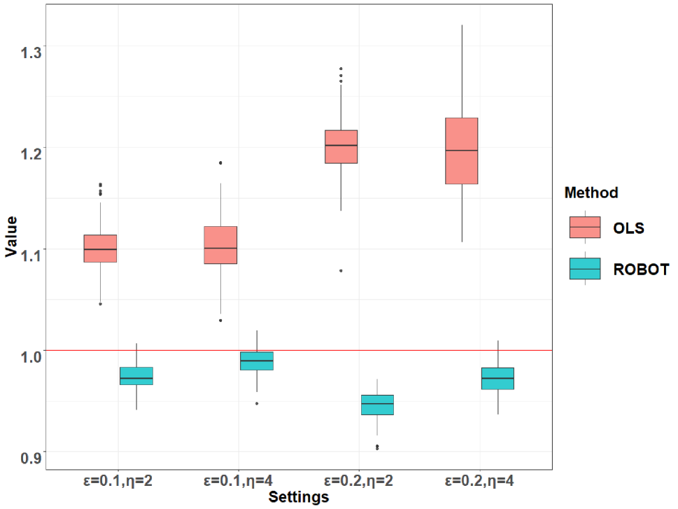
(a) boxplots of slope ($\alpha$) estimates in different situation

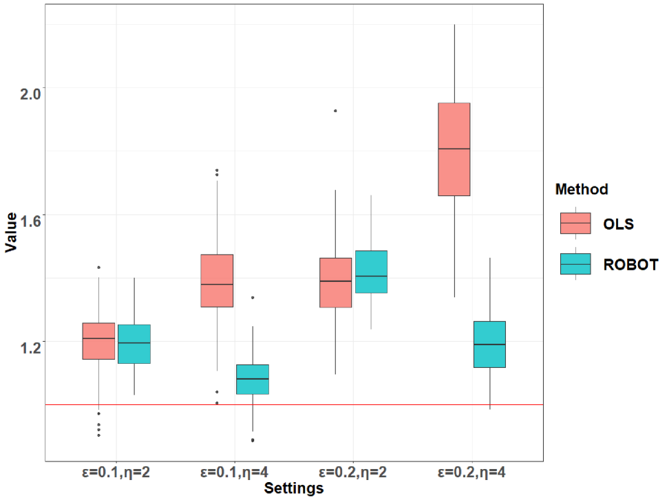
(b) boxplots of intercept ($\beta$) estimates in different situation

Figure 6: We show the estimated effect of parameters through boxplots. The red lines represent the true values of the model parameters.

For the estimation of $\alpha$, Figure 6(a) shows that the OLS is greatly affected by the outliers: both the bias and variance increase rapidly with the size and proportion of the outliers. The ROBOT, on the contrary, shows great robustness against the outliers, with much smaller bias and variance. For the estimation of $\beta$ (Figure 6(b)), ROBOT and OLS have similar performance for $\eta=2$, but ROBOT outperforms OLS when the contamination size is large.

The purpose of our construction of outlier robust estimation is to let the trained model close to the uncontaminated model (33), hence it can fit better the data generated from (33). We, therefore, consider calculating mean square error (MSE) with respect to the data generated from (33), in order to compare the performance of the OLS and ROBOT.

In simulation, we set $n=1000$, $\sigma=1$, $\alpha=1$, $\beta=1$ and change the contamination size $\eta$. Each experiment is repeated $100$ times. In Figures 7(a) and 7(b), we plot the averaged MSE of the OLS and ROBOT against $\eta$ for $\varepsilon=0.1$ and $\varepsilon=0.2$, respectively. Even a rapid inspection of Figures 7(a) and 7(b) demonstrates the better performance of ROBOT than the OLS. Specifically, in both figures, OLS is always above ROBOT, and the latter yields much smaller MSE than the former for a large $\eta$. After careful observation, it is found that when the proportion of outliers is small, the MSE curve of ROBOT is close to 1, which is the variance of the data itself. The results show that ROBOT has good robustness against outliers of all sizes.

ROBOT, with the ability to detect outliers, hence fits the uncontaminated distribution better than OLS. Next, we use Figure 8(a) and Figure 8(b) to show Algorithm 1 enables us to detect outliers accurately and hence makes the estimation procedure more robust. More specifically, we can see there are many points in Figure 8(a) (after 1 iteration) classified incorrectly; after 10 iterations (Figure 8(b)), only a few outliers close to the uncontaminated distribution are not detected.

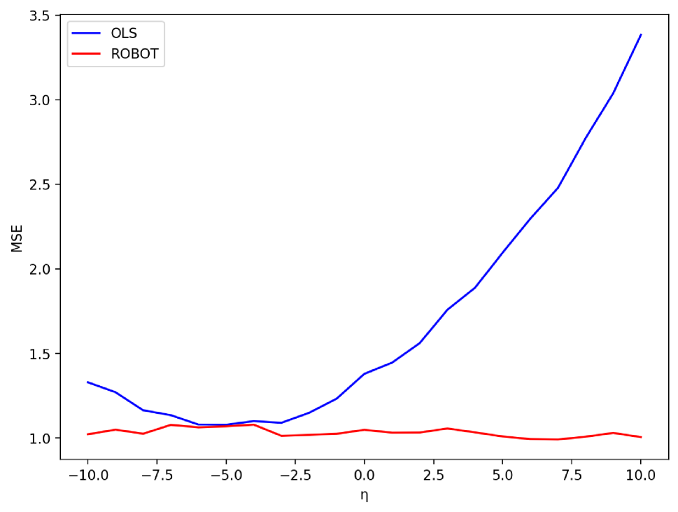
(a) MSE ($p=0.1$)

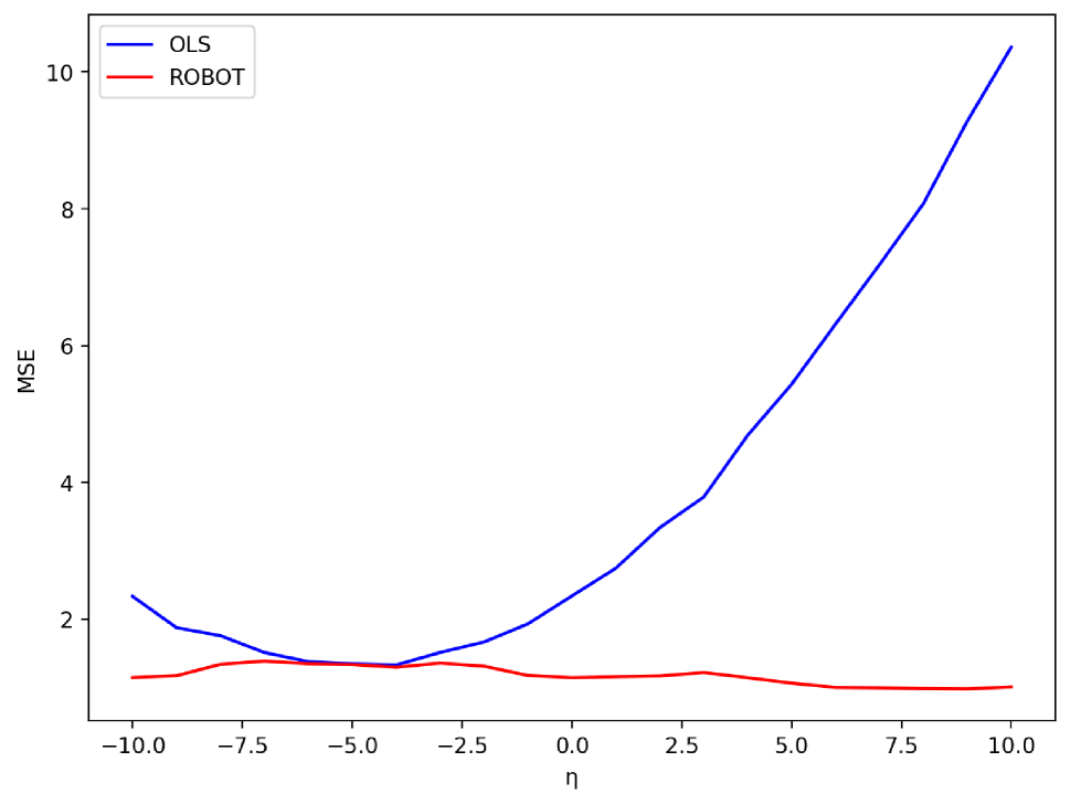
(b) MSE ($p=0.2$)

Figure 7: We consider using MSE based on the uncontaminated data to show how well the estimate fits the real distribution. The left picture is the MSE corresponding to different scale parameter $\eta$ when the proportion of outliers is 0.1. The red line represents ROBOT-based estimation while the blue line represents OLS. On the right is the result when $\varepsilon=0.2$.

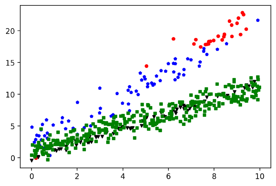
(a) iteration=1

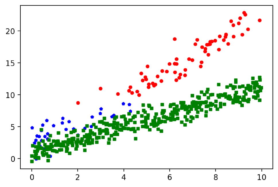
(b) iteration=10

Figure 8: Outlier detection for ROBOT-based estimation: the left panel is the result after 1 iteration in Algorithm 1, and the right panel is the result after 10 iterations. Circle points (red) and square points (green) represent the outliers and uncontaminated points correctly detected respectively; pentagon points (blue) and inverted triangle (black) represent the outliers and uncontaminated points incorrectly detected. (Simulation settings: $n=500$, $\varepsilon=0.2$ and $\eta=1$).

C.2 RWGAN

RWGAN-2 Here we provide the key steps needed to implement the RWGAN-2, which is derived directly from (3). Noticing that (3) allows the distribution of reference samples to be modified, and there is a penalty term to limit the degree of the modification, the RWGAN-2 can thus be implemented as follows.

Letting ${X}^{\prime}\sim\mathrm{P}_{{\rm r}^{\prime}}$, where $\mathrm{P}_{{\rm r}^{\prime}}$ is the modified reference distribution, and other notations be the same as in (15), the objective function of the RWGAN-2 is defined as

$$\min_{\theta}\min_{\mathrm{P}_{{\rm r}^{\prime}}}\sup_{\|f_{\xi}\|_{L}\leq 1,{\rm range}(f_{\xi})\leq 2\lambda}\left\{{\rm E}[f_{\xi}({X}^{\prime})]-{\rm E}[f_{\xi}(G_{\theta}({Z}))]+\lambda_{\rm m}\|\mathrm{P}_{{\rm r}}-\mathrm{P}_{{\rm r}^{\prime}}\|_{\rm TV}\right\},$$ (34)

where $\lambda_{\rm m}$ is the penalty parameter to control the modification. The algorithm for implementing the RWGAN-2 is summarized in Algorithm 2. Note that in Algorithm 2, we consider introducing a new neural network $U_{\omega}$ to represent the modified reference distribution, which corresponds to $\mathrm{P_{r^{\prime}}}$ in the objective function (34). Then we can follow (34) and use standard steps to update generator, discriminator and modified distribution in turn. Here are a few things to note: (i) from the objective function, we know that the loss function of discriminator is ${\rm E}[f_{\xi}(G_{\theta}({Z}))]-{\rm E}[f_{\xi}({X}^{\prime})]$, the loss function of modified distribution is ${\rm E}[f_{\xi}({X}^{\prime})]+\lambda_{\rm m}\|\mathrm{P}_{{\rm r}}-\mathrm{P}_{{\rm r}^{\prime}}\|_{\rm TV}$ and the loss function of generator is $-{\rm E}[f_{\xi}(G_{\theta}({Z}))]$; (ii) we truncate the absolute values of the discriminator parameter $\xi$ to no more than a fixed constant $c$ on each update: this is a simple and efficient way to satisfy the Lipschitz condition in WGAN; (iii) we adopt Root Mean Squared Propagation (RMSProp) optimization method which is recommended by Arjovsky et al. (2017) for WGAN.

Algorithm 2 RWGAN-2

0:  observations $\{{X}_{1},{X}_{2},\ldots,{X}_{n}\}$, critic $f_{\xi}$ (indexed by a parameter $\xi$), generator $G_{\theta}$ (indexed by a parameter $\theta$), modified distribution $U_{\omega}$ (indexed by a parameter $\omega$), learning rate $\alpha$, modification penalty parameter $\lambda_{\rm m}$, batch size $N_{\rm batch}$, number of iterations $N_{\rm iter}$, noise distribution $\mathrm{P}_{{z}}$, clipping parameter $c$.

1:  while $i\leq N_{\rm iter}$ do

2:     sample a batch of reference samples $\{{X}_{i}\}_{i=1}^{N_{\rm batch}}$;

3:     sample a batch of i.i.d. noises $\{{Z}_{i}\}_{i=1}^{N_{\rm batch}}\sim\mathrm{P}_{{z}}$;

4:     let ${L}_{\xi}=\frac{1}{N_{\rm batch}}\sum_{i}f_{\xi}(G_{\theta}({Z}_{i}))-\sum_{i}U_{\omega}({X}_{i})f_{\xi}({X}_{i})$;

5:     update $\xi\xleftarrow{}\xi-\alpha\cdot RMSProp(\xi,\nabla_{\xi}{L}_{\xi})$;

6:     $\xi\xleftarrow{}\mathrm{clip}(\xi,-c,c)$;

7:     let ${L}_{\theta}=-\frac{1}{N_{\rm batch}}\sum_{i}f_{\xi}(G_{\theta}({Z}_{i}))$;

8:     update $\theta\xleftarrow{}\theta-\alpha\cdot RMSProp(\theta,\nabla_{\theta}{L}_{\theta})$;

9:     let ${L}_{\omega}=\sum_{i}U_{\omega}({X}_{i})f_{\xi}({X}_{i})+\lambda_{\rm m}\sum_{i}|U_{\omega}({X}_{i})-1/N_{\rm batch}|$;

10:     update $\omega\xleftarrow{}\omega-\alpha\cdot RMSProp(\omega,\nabla_{\omega}{L}_{\omega})$.

11:  end while

11:  generation model $G_{\theta}$

Some details. If we assume that the reference sample is $m$-dimensional, the generator is a neural network with $m$ input nodes and $m$ output nodes; the critic is a neural network with $m$ input nodes and $1$ output node. Also, in RWGAN-2 and RWGAN-B, we need an additional neural network (it has $m$ input nodes and $1$ output node) to represent the modified distribution. In both the synthetic data example and Fashion-MNIST example, all generative adversarial models are implemented based on $\mathsf{Pytorch}$ (an open source Python machine learning library https://pytorch.org/) to which we refer for additional computational details.

In RWGAN-1, as in the case of WGAN, we also only need two neural networks representing generator and critic, but we need to make a little modification to the activation function of the output node of critic: (i) choose a bounded activation function (ii) add a positional parameter to the activation function. This is for $f_{\xi}$ to satisfy the condition $\mathrm{range}(f_{\xi})\leq 2\lambda$ in (16). So RWGAN-1 has a simple structure similar to WGAN, but still shows good robustness to outliers. We can also see this from the objective functions of RWGAN-1 ((16)) and RWGAN-2 ((34)): RWGAN-2 needs to update one more parameter $\omega$ than RWGAN-1. This means more computational complexity.

In addition, we make use of Fashion-MNIST to provide an example of how generator $G_{\theta}$ works on real-data. We choose a standard multivariate normal random variable (with the same dimension as the reference sample) to obtain the random input sample. An image in Fashion-MNIST is of $28\times 28$ pixels, and we think of it as a 784-dimensional vector. Hence, we choose a $784$-dimensional standard multidimensional normal random variable $Z$ as the random input of the generator $G_{\theta}$, from which we output a vector of the same 784 dimensions (which corresponds to the values of all pixels in a grayscale image) to generate one fake image. To understand it in another way, we can regard each image as a sample point, so all the images in Fashion-MNIST constitute an empirical reference distribution $\hat{\mathrm{P}}_{\rm r}$, thus our goal is to train $G_{\theta}$ such that $\mathrm{P}_{\theta}$ is very close to $\hat{\mathrm{P}}_{\rm r}$.

Appendix D The choice of $\lambda$

D.1 Some considerations based on RWGAN

Here we focus on the applications of RWGAN and MERWE and illustrate, via Monte Carlo experiments, how $\lambda$ would affect the results. First, we recall the experiment in § 5.2.1: MERWE of location for sum of log-normal. We keep other conditions unchanged, and just change the parameter $\lambda$ to see how the estimated value changes. We set $n=200$, $\varepsilon=0.1$ and $\eta=4$ and other parameters are still set as in § 5.2.1. The result is shown in Figure 9. We can observe that the MSE is large when $\lambda$ is small. The reason for this is that we truncate the cost matrix prematurely at this time, making robust Wasserstein distance unable to distinguish the differences between distributions. When $\lambda$ is large, there is negligible difference between Wasserstein distance and robust Wasserstein distance, resulting in almost the same MSE estimated by MERWE and MEWE. When $\lambda$ is moderate, within a large range (e.g., from $\exp(2)$ to $\exp(5.5)$), the MERWE outperforms the MEWE.

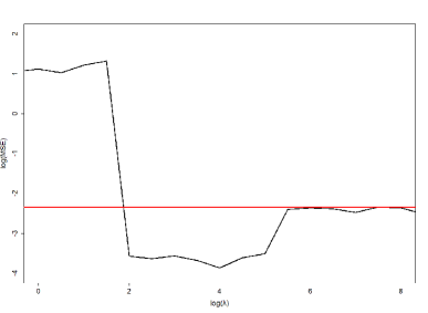
Figure 9: $\log(\rm MSE)$ of MERWE based on 1000 times experiment for different values of $\log(\lambda)$. The horizontal (red) line represents $\log(\rm MSE)$ of MEWE.

We consider a novel way to study parameter selection based on our Theorem 1, which implies that modifying the constraint on $\mathrm{range}(\psi)$ is equivalent to changing the parameter $\lambda$ in equation (4). This reminds us that we can use RWGAN-1 to study how to select $\lambda$.

We consider the same synthetic data as in § C.2 and set $n=1000,\varepsilon=0.1$ and $\eta=2$. To quantify training quality of RWGAN-1, we take the Wasserstein distance of order 1 between the clean data and data generated from RWGAN-1. Specifically, we draw 1000 samples from model (17) and generate 1000 samples from the model trained by RWGAN-1 with different parameter $\lambda$. Then, we calculate the empirical Wasserstein distance of order 1 between them. The plot of the empirical Wasserstein distance against $\log(\lambda)$ is shown in Figure 10. The Wasserstein distance has a trend of decreasing first and increasing later on: it reaches the minimum at $\log(\lambda)=-2$. Also, we notice that over a large range of $\lambda$ values (i.e. from $\exp(-4)$ to $\exp(0)$), the Wasserstein distance is small: this illustrates that RWGAN-1 has a good outlier detection ability for a choice of the penalization parameter within this range.

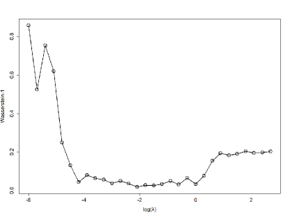
Figure 10: Plot of the empirical Wasserstein distance of order 1 between the clean data and data generated from RWGAN-1 for different values of $\log(\lambda)$.

Heuristically, a large $\lambda$ means the truncated cost function is just slightly different from the non-truncated one. Therefore, RWGAN-1 will be greatly affected by outliers. When $\lambda$ is small, the cost function is severely truncated, which means that we are modifying too much of the distribution. This deviates from our main purpose of GAN (i.e., $\mathrm{P_{r}}\approx\mathrm{P_{\theta}}$). Hence, the distribution of final outputs generated from RWGAN-1 becomes very different from the reference one.

Both experiments suggest that to achieve good performance of ROBOT, one could choose a moderate $\lambda$ within a large range. Actually, the range of a “good” $\lambda$ depends on the size and proportion of outliers: When the size and proportion are close to zero, both moderate and large $\lambda$ will work well, since only slight or no truncation of the cost function is needed; when the size and proportion are large, a large truncation is needed, so this range becomes smaller. Generally, we prefer to choose a slightly larger $\lambda$, as we found in the experiment that when we use a larger $\lambda$, the performance of ROBOT is at least no worse than that using OT.

D.2 Selection based on concentration inequality

Methodology. In the Monte Carlo setting of Section 5.2.1, Figure 9 in Appendix D.1 illustrates that MERWE has good performance (in terms of MSE) when $\lambda$ is within the range $[\exp(2),\exp(5)]$. The estimation of the MSE represents, in principle, a valuable criterion that one can apply to select $\lambda$. However, while this idea is perfectly fine in the case of synthetic data, its applicability seems to be hard in real data examples, where the true underling parameter is not known. To cope with this issue, Warwick and Jones (2005) propose to use a pilot estimators which can yield an estimated MSE. The same argument can be considered also for the our estimator, but this entails the need for selecting a pilot estimator: a task that cannot be easy for some complex models and for the models considered in this paper. Therefore, we propose and investigate the use of an alternative approach, which yields a range of values of $\lambda$ similar to the one obtained computing the MSE but it does not need to select such a pilot estimator.

To start with, let us consider that Th. 7 yields that $\left|W^{\lambda}(\hat{\mu}_{n},\mu^{\ast})-{\rm E}[W^{\lambda}(\hat{\mu}_{n},\mu^{\ast})]\right|$ exceeds, in the presence of contamination, the threshold

$$\sigma\sqrt{\frac{|I|}{n}}\sqrt{\frac{2t}{n}}+\frac{4\lambda t}{n}+\frac{4\lambda|O|}{n}$$ (35)

with probability bounded by $2\exp(-t)$. Moreover, in the absence of contamination ($|O|=0$ and $|I|=n$), the mean concentration in (9) implies that $\left|W^{\lambda}(\hat{\mu}_{n},\mu^{\ast})-{\rm E}[W^{\lambda}(\hat{\mu}_{n},\mu^{\ast})]\right|$ takes on values larger than the threshold

$$\sigma\sqrt{\frac{2t}{n}}+\frac{4\lambda t}{n}.$$ (36)

with the same probability upper bound.

Then, to select $\lambda$ we propose to set up the following criterion, which compares the changes in (35) and (36) due to different values of $\lambda$. More in detail, for a fixed $t>0$, we assume a contamination level $\tau$ which represents a guess that the statistician does about the actual level of data contamination. Then we compare the thresholds of the uncontaminated and contaminated data at different values of $\lambda$. To this end, we compute the ratio between the thresholds in (36) and (35) and define

$$\mathcal{Q}(n,\tau,\lambda,t):=\frac{\sigma\sqrt{\frac{2t}{n}}+\frac{4\lambda t}{n}}{\sigma\sqrt{1-\tau}\sqrt{\frac{2t}{n}}+\frac{4\lambda t}{n}+4\tau\lambda}.$$

Assuming that $\sigma$ is a twice differentiable function of $\lambda$, one can check that $\mathcal{Q}$ decreases monotonically in $\lambda$. Next we explain how ${\partial\mathcal{Q}}/{\partial\lambda}$ can be applied to define a data driven criterion for the selection of $\lambda$.

We remark that for most models, the computation of $\mathcal{Q}$ and of ${\partial\mathcal{Q}}/{\partial\lambda}$ need to be performed numerically. To illustrate this aspect and to elaborate further on the selection of $\lambda$, we consider the same Monte Carlo setting of Section 5.2.1, where $\varepsilon={|O|}/{n}$ is the actual contamination level. In Appendix D.1, we found through numerical experiments that MERWE has good performance for $\lambda$ within the $[\exp(2),\exp(5)]$. Hence, in our numerical analysis, we consider this range as a benchmark for evaluating the $\lambda$ selection procedure based on $\mathcal{Q}(n,\tau,\lambda,t)$. Moreover, we need to specify a value for the contamination level and fix $t$. In our numerical analysis we set $\tau=0.1$ and $t=1$—we remark that the specified $\tau$ coincides with the percentage of outliers $\varepsilon$: later on we discuss the case when $\tau\neq\varepsilon$. In Figure 11, we display the plot of $\mathcal{Q}$ with respect to $\lambda$: $\mathcal{Q}$ decreases monotonically, with slope which decreases as $\lambda\to\infty$. The plot suggests that, when $\lambda$ is small, $\mathcal{Q}$ decreases fast for small increments in the value of $\lambda$. This is due to the fact that, for $\lambda$ small, a small change of $\lambda$ has a large influence on the transport cost $c^{(\lambda)}$ and hence on the values of $W^{(\lambda)}$. On the contrary, when $\lambda$ is sufficiently large, larger values of the trimming parameter do not have large influence on the transport cost $c^{(\lambda)}$. As a result, looking at the (estimated) slope of (estimated) $\mathcal{Q}$ allows to identify a range of $\lambda$ values which avoids the small values (for which $W^{(\lambda)}$ trims too many observations and it is maximally concentrated about its mean) and large values (for which $W^{(\lambda)}$ trims too few observations and it is minimally concentrated about its mean). This is the same information available in Figure 9, but differently from the computation which yields the MSE in that figure, our method does not entail either the need for knowing the true value of the model parameter or the need for a pilot estimator.

Implementation. Operationally, to obtain the desired range of $\lambda$ values, one needs to create a sequence of $\{\lambda_{k}\}$ with $0<\lambda_{1}<\lambda_{2}<\ldots<\lambda_{N},\,N>1$. Then, one computes the sequence of absolute slopes

$$\mathrm{AS}{(n,\tau,\lambda_{k},t)}=\frac{|{\mathcal{Q}}{(n,\tau,\lambda_{k+1},t)}-{\mathcal{Q}}{(n,\tau,\lambda_{k},t)}|}{\lambda_{k+1}-\lambda_{k}},k\geq 1,$$

at different values of $\lambda_{k}$. We remark that to compute $\mathrm{AS}$, we need to estimate $\sigma^{2}$. To this end, a robust estimator of the variance should be applied. In our numerical exercises, we find numerically convenient to fix $X_{i}^{\prime}$ to $\bar{X}_{\mathrm{rob}}$ which represents the geometric median for real-valued variable $X$. Then, we replace $\rm{E}\left[\min\left(d^{2}\left(X_{i},X_{i}^{\prime}\right),(2\lambda)^{2}\right)\right]$ by $({1}/{n})\sum_{i=1}^{n}\min\left\{d^{2}\left(X_{i},\bar{X}_{\mathrm{rob}}\right),(2\lambda)^{2}\right\}$.

Once the different values of AV are available, one needs to make use of them to select $\lambda$. To this end, we propose to follow the idea of Algorithm 1 in La Vecchia et al. (2015) and choose $\lambda^{\star}:=\min\left\{\lambda_{k}:{\mathrm{AS}}{(n,\tau,\lambda_{i},t)}\leq\iota,\text{for all }\lambda_{i}\geq\lambda_{k}\right\}$, where $\iota$ is a user-specified value. According to our numerical experience it is sensible to specify values of $\iota$ which are close to zero: they typically define estimators having a performance that remains stable across different Monte Carlo settings, while avoiding to trim too many observations. For the sake of illustration, in Figure 12 we display the estimated AS related to $\mathcal{Q}$ as in Figure 11: we see that its maximum value is around 0.05. We propose to set $\iota=0.001$: this value is slightly larger than zero (namely, the value that $\mathrm{AS}$ has when $\lambda$ is large). This yields $\lambda^{\star}\approx 26$ ($\ln\lambda\approx 3.25$), which is within the range $[\exp(2),\exp(5)]$ where MERWE produces small MSE as displayed in Figure 9. A reassuring aspect emerges from Figure 12: in case one decides to set slightly larger values of $\iota$ (e.g. values between $0.008$ and $0.001$), the selection procedure is still able to provide a value of $\lambda^{\star}$ within the benchmark $[\exp(2),\exp(5)]$. Essentially, we conclude that any value of $\iota$ which is greater than zero and smaller than the max of AS selects a $\lambda^{\star}$ which in turns yields a good performance (in terms of MSE) of our estimator.

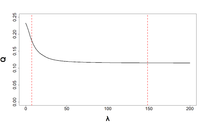
Figure 11: The curve (black) of $\mathcal{Q}$ with respect to $\lambda$. The coordinates of the vertical dashed lines (red) are $\exp(2)$ and $\exp(5)$, respectively.

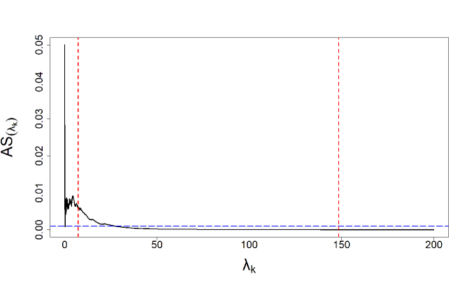
Figure 12: Plot of the $\mathrm{AS}$ curve (black) as a function of $\lambda$. The coordinates of the vertical dashed lines (red) are $\exp(2)$ and $\exp(5)$, respectively, and the coordinate of horizontal dashed line (blue) is $0.001$.

Remark. We mention three interesting methodological aspects related to this selection procedure. First, the proposed criterion is based on the computation of $\mathrm{AS}$ for different $\lambda_{k}$ and it does not entail the need for computing the corresponding MDE $\hat{\theta}^{\lambda}_{n}$. This aspect makes our criterion easy-to-implement and fast. Second, one may wonder what is the distribution of $\lambda^{\ast}$ when many samples from the same $O\cup I$ setting are available. Put it in another way, given many samples and selecting in each sample $\lambda$ by the aforementioned procedure how does $\lambda^{\ast}$ change? Third, an interesting question related to the proposed criterion is: what happens to $\lambda^{\ast}$ if the statistician specifies a contamination level $\tau$ that is different from the true contamination level $\varepsilon$? As far as the last two questions are concerned, we remark that Figure 12 is based on one sample and it cannot answer these questions. Thus, to gain deeper understanding, we keep the same setting as in the Monte Carlo experiment (which yielded Figure 12) and we simulate 1000 samples, specifying $\tau=0.05,0.1,0.2$ and selecting $\lambda^{\star}$ by the aforementioned procedure. In Figure 13 we display the kernel density estimates of the selected values. The plots illustrate that, for each $\tau$ value, the kernel density estimate is rather concentrated: for instance, if $\tau=0.1$ the support of the estimated density goes from about 3 to about 3.4. Moreover, looking at the estimated densities when $\tau=0.005$ (underestimation of the number of outliers) and $\tau=0.2$ (overestimation of the number of outliers), we see that, even if $\tau\neq\varepsilon$, the selection criterion still yields values of $\lambda$ which are within the benchmark range $[\exp(2),\exp(5)]$.

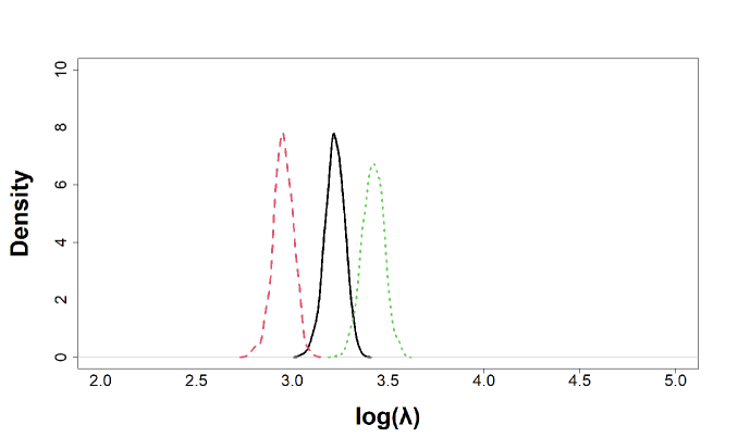
Figure 13: Dashed line (red), solid line (black), dotted line (green) represent the Gaussian kernel density functions (bandwidth = $0.0167$) of $\log(\lambda^{\star})$ for $\tau=0.05,0.1,0.2$, respectively.

Appendix E Domain adaptation

Methodology. Domain adaptation is a fundamental problem in machine learning and has attracted extensive attention in the past decade. Domain adaptive learning aims at solving the learning problem of the inconsistent probability distribution of training samples and test samples. It has a wide range of applications in natural language processing (Ramponi and Plank (2020)), text analysis (Daumé III (2009)) and medical data analysis (Hu et al. (2020)). Some effective works based on OT approach have recently been proposed. For instance, Kersting and Železnỳ (2013) assume that there exists a transformation between the source and target distributions and they use an entropy-regularized optimal transport to find this transformation.

The domain adaptation problem can be stated as follows. Let $\{({X}_{i}^{\rm s},Y_{i}^{\rm s});1\leq i\leq N_{\rm s}\}$ denote an i.i.d. sequence of source samples and $\{({X}_{j}^{\rm t},Y_{j}^{\rm t});1\leq j\leq N_{\rm t}\}$ denote an i.i.d. sequence of target samples, which have joint distributions ${\rm P_{s}}$ and ${\rm P_{t}}$ (${\rm P_{s}}$ and ${\rm P_{t}}$ are possibly different), respectively. In the context of domain adaptation, we are interested in estimating the label $Y_{j}^{\rm t},j=1,\ldots,N_{\rm t},$ from observations $\{({X}_{i}^{\rm s},Y_{i}^{\rm s});1\leq i\leq N_{\rm s}\}$ and $\{{X}_{j}^{\rm t};1\leq j\leq N_{\rm t}\}$. Therefore, the aim is to find a function $f$ that predicts the target label values. Courty et al. (2017) assume that there is a transformation $\mathcal{T}$ between ${\rm P}_{\rm s}$ and ${\rm P}_{\rm t}$, which can be estimated by OT.

In practice, since the population distribution of the source sample is unknown, it is usually estimated by its empirical counterpart $\widehat{\rm P}_{\rm s}^{(N_{\rm s})}={N_{\rm s}}^{-1}\sum_{i=1}^{N_{\rm s}}\delta_{{X}_{i}^{\rm s},Y_{i}^{\rm s}}.$ On the target domain, supposing we can obtain a function $f$ to predict the unobserved response variable $Y^{\rm t}$, then the empirical distribution of the target sample is $\widehat{{\rm P}}_{{\rm t};f}^{(N_{\rm t})}=N_{\rm t}^{-1}\sum_{j=1}^{N_{\rm t}}\delta_{{{X}}_{j}^{\rm t},f({{X}}_{j}^{\rm t})}.$ The original problem then becomes finding a function $f$ that minimizes the transport cost between the joint source distribution $\widehat{\rm P}_{\rm s}^{(N_{\rm s})}$ and an estimated joint target distribution $\widehat{{\rm P}}_{{\rm t};f}^{(N_{\rm t})}$.

Courty et al. (2017) define the cost function ${D}\left({X}_{1},Y_{1};{X}_{2},Y_{2}\right)=\alpha{d}\left({X}_{1},{X}_{2}\right)+{L}\left(Y_{1},Y_{2}\right),$ where ${L}$ is a loss function that measures the discrepancy between $Y_{1}$ and $Y_{2}$ and $\alpha$ is a positive parameter that balances the metric $d$ in the feature space and the loss ${L}$. We want to reduce the spatial distance between the source and target domains. Thus, the optimization problem becomes

$$\min_{f}W\left(\hat{\mathrm{P}}_{\rm s}^{(N_{\rm s})},\hat{\mathrm{P}}_{{\rm t};f}^{(N_{\rm t})}\right)\equiv\min_{f,\mathbf{\Pi}}\sum_{ij}{D}\left({X}_{i}^{\rm s},Y_{i}^{\rm s};{X}_{j}^{\rm t},f({X}_{j}^{\rm t})\right)\mathbf{\Pi}_{ij}^{(N_{\rm s},N_{\rm t})}$$ (37)

Courty et al. (2014) propose that if optimal transport matrix $\mathbf{\Pi}^{(N_{\rm s},N_{\rm t})}$ between $\widehat{\rm P}_{\rm s}^{(N_{\rm s})}$ and $\widehat{{\rm P}}_{{\rm t};f}^{(N_{\rm t})}$ is fixed, and ${L}$ is the squared-loss, the learning problem (37) for regression boils down to

$$\min_{f}N_{\rm t}^{-1}\sum_{j=1}^{N_{\rm t}}\left\|\hat{Y}_{j}-f(X_{j}^{\rm t})\right\|^{2}$$ (38)

where $\hat{Y}_{j}=N_{\rm t}\sum_{i=1}^{N_{\rm s}}\mathbf{\Pi}_{ij}^{(N_{\rm s},N_{\rm t})}Y_{i}^{\rm s}$. Courty et al. (2014) propose to update $f$ and $\mathbf{\Pi}^{(N_{\rm s},N_{\rm t})}$ in turn to obtain the $f$ that minimizes (37).

Given that ROBOT is a robust version of OT, it can naturally be applied to this domain adaptation problem. In particular, we use ROBOT instead of OT to get the transport matrix, and at the same time use ROBOT to detect outliers. Specific details are given in Algorithm 3.

Algorithm 3 ROBUST DOMAIN ADAPTATION

0:  source sample $\{({X}_{i}^{\rm s},Y_{i}^{\rm s}),1\leq i\leq N_{\rm s}\}$, target features $\{{X}_{j}^{\rm t},1\leq j\leq N_{\rm t}\}$, robust regularization parameter $\lambda$, parametric model $f_{\theta}$ (index by a parameter $\theta$).

1:  estimate $\theta$ using the source sample;

2:  while ${\theta}$ does not convergence do

3:     let $C^{(\lambda,N_{\rm s},N_{\rm t})}_{ij}=\min\left\{{D}\left({X}_{i}^{\rm s},Y_{i}^{\rm s};{X}_{j}^{\rm t},f_{\theta}\left({X}_{j}^{\rm t}\right)\right),2\lambda\right\}$;

4:     based on the cost matrix $(C^{(\lambda,N_{\rm s},N_{\rm t})}_{ij})_{1\leq i\leq N_{\rm s},1\leq j\leq N_{\rm t}}$, compute the optimal transport plan matrix $\mathbf{\Pi}^{(N_{\rm s},N_{\rm t})}$, and collect the set of all indices

$$\mathcal{I}=\{(i,j):{D}\left({X}_{i}^{\rm s},Y_{i}^{\rm s};{X}_{j}^{\rm t},f_{\theta}\left({X}_{j}^{\rm t}\right)\right)\geq 2\lambda,1\leq i\leq N_{\rm s},1\leq j\leq N_{\rm t}\}.$$

5:     set $s(i)=-\sum_{j=1}^{N_{\rm t}}\mathbf{\Pi}^{(N_{\rm s},N_{\rm t})}_{ij}\mathbbm{1}_{(i,j)\in\mathcal{I}}$, and find $\mathcal{H}$, the set of all the indices where $s(i)+1/N_{\rm s}=0$;

6:     remove $\ell$-th row of $\mathbf{\Pi}^{(N_{\rm s},N_{\rm t})}$ for all $\ell\in\mathcal{H}$ and normalize the matrix over columns to form a new matrix $\mathbf{\Pi}^{(N^{\prime}_{\rm s},N_{\rm t})}$;

7:     let ${L}_{\theta}=N_{\rm t}^{-1}\sum_{j=1}^{N_{\rm t}}\left\|\hat{Y}_{j}-f_{\theta}(X_{j}^{\rm t})\right\|^{2}$, where $\hat{Y}_{j}=N_{\rm t}\sum_{i=1}^{N^{\prime}_{\rm s}}\mathbf{\Pi}_{ij}^{(N^{\prime}_{\rm s},N_{\rm t})}Y_{i}^{\rm s}$;

8:     update $\theta$, which minimizes ${L}_{\theta}$.

9:  end while

9:  Model $f_{\theta}$

Monte Carlo experiments. We consider the setting where the $N_{\rm s}$ source samples are generated from

$$\begin{array}[]{cc}&X_{i}^{(N_{\rm s})}\sim\mathcal{N}(-2,1),i=1,2,\ldots,[N_{\rm s}/2],\\ &X_{i}^{(N_{\rm s})}\sim\mathcal{N}(2,1),i=[N_{\rm s}/2]+1,[N_{\rm s}/2]+2,\ldots,N_{\rm s},\\ &Y_{i}^{(N_{\rm s})}=\sin(X_{i}^{(N_{\rm s})}/2)+Z_{i}^{(N_{\rm s})},i=1,2,\ldots,[9N_{\rm s}/10],\\ &Y_{i}^{(N_{\rm s})}=\sin(X_{i}^{(N_{\rm s})}/2)+2+Z_{i}^{(N_{\rm s})},i=[9n/10]+1,[9N_{\rm s}/10]+2,\ldots,N_{\rm s},\\ &Z_{i}^{(N_{\rm s})}\sim\mathcal{N}(0,0.1^{2})\\ \end{array}$$ (39)

and the $N_{\rm t}$ target samples are generated from

$$\begin{array}[]{cc}&X_{j}^{(N_{\rm t})}\sim\mathcal{N}(-1,1),j=1,2,\ldots,[N_{\rm t}/2],\\ &X_{j}^{(N_{\rm t})}\sim\mathcal{N}(2,1),j=[N_{\rm t}/2]+1,[N_{\rm t}/2]+2,\ldots,N_{\rm t},\\ &Y_{j}^{(N_{\rm t})}=\sin((X_{i}^{(N_{\rm t})}-2)/2)+Z_{i}^{(N_{\rm t})},j=1,2,\ldots,N_{\rm t},\\ &Z_{j}^{(N_{\rm t})}\sim\mathcal{N}(0,0.1^{2}).\\ \end{array}$$ (40)

Since $Y_{j}^{(N_{\rm t})},j=1,2,\ldots,N_{\rm t},$ is unknown, we need to estimate the relationship $f$ between $X$ and $Y$ on the target domain as accurately as possible. In simulation, we set $N_{\rm s}=200$ and $N_{\rm t}=200$. We compare three methods for estimating $f$: the first one is the Kernel Ridge Regression (KRR); the second one proposed by Courty et al. (2017) is a combination of OT and KRR; the third one is the revision of the second method, using ROBOT instead of OT.

Figure 14 shows that the source samples and target samples have a similar type of distribution but there is a drift between them. Also, there are some obvious outliers in the source samples. We find the curve yielded by KRR, which uses only the source samples information and hence fits nicely the source samples, looks far away from the target samples. This is due to the drift between the target and source distributions. The result given by the method in Courty et al. (2017) is closer to the target data, but because of outliers, it does not perform well in the tails. Our method yields estimates that fit the target distribution significantly better than the other competitors.

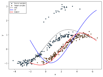
Figure 14: Scatter plots of the source and target samples, and functions estimated by different approaches. The grey-blue points represent the source samples (Some outliers appear in source samples) and the orange points represent the target samples. The gray, blue and red curves are the estimates of the KRR, the method of Courty et al. (2017) and our method, respectively.

References

- Alvarez-Esteban et al. (2008) Alvarez-Esteban, P. C., E. Del Barrio, J. A. Cuesta-Albertos, and C. Matran (2008). Trimmed comparison of distributions. Journal of the American Statistical Association 103(482), 697–704.
- Amari et al. (2018) Amari, S.-i., R. Karakida, and M. Oizumi (2018). Information geometry connecting Wasserstein distance and Kullback–Leibler divergence via the entropy-relaxed transportation problem. Information Geometry 1(1), 13–37.
- Arjovsky et al. (2017) Arjovsky, M., S. Chintala, and L. Bottou (2017). Wasserstein generative adversarial networks. In International conference on machine learning, pp. 214–223. PMLR.
- Balaji et al. (2020) Balaji, Y., R. Chellappa, and S. Feizi (2020). Robust optimal transport with applications in generative modeling and domain adaptation. Advances in Neural Information Processing Systems 33, 12934–12944.
- Bassetti et al. (2006) Bassetti, F., A. Bodini, and E. Regazzini (2006). On minimum Kantorovich distance estimators. Statistics & probability letters 76(12), 1298–1302.
- Bassetti and Regazzini (2006) Bassetti, F. and E. Regazzini (2006). Asymptotic properties and robustness of minimum dissimilarity estimators of location-scale parameters. Theory of Probability & Its Applications 50(2), 171–186.
- Basu et al. (2011) Basu, A., H. Shioya, and C. Park (2011). Statistical inference: the minimum distance approach. CRC press.
- Bernton et al. (2019) Bernton, E., P. E. Jacob, M. Gerber, and C. P. Robert (2019). On parameter estimation with the Wasserstein distance. Information and Inference: A Journal of the IMA 8(4), 657–676.
- Boissard and Le Gouic (2014) Boissard, E. and T. Le Gouic (2014). On the mean speed of convergence of empirical and occupation measures in wasserstein distance. 50(2), 539–563.
- Bolley et al. (2007) Bolley, F., A. Guillin, and C. Villani (2007). Quantitative concentration inequalities for empirical measures on non-compact spaces. Probability Theory and Related Fields 137(3), 541–593.
- Brenier (1987) Brenier, Y. (1987). Décomposition polaire et réarrangement monotone des champs de vecteurs. CR Acad. Sci. Paris Sér. I Math. 305, 805–808.
- Carriere et al. (2017) Carriere, M., M. Cuturi, and S. Oudot (2017). Sliced Wasserstein kernel for persistence diagrams. In International conference on machine learning, pp. 664–673. PMLR.
- Chizat (2017) Chizat, L. (2017). Unbalanced optimal transport: Models, numerical methods, applications. Ph. D. thesis, Université Paris sciences et lettres.
- Courty et al. (2017) Courty, N., R. Flamary, A. Habrard, and A. Rakotomamonjy (2017). Joint distribution optimal transportation for domain adaptation. Advances in Neural Information Processing Systems 30.
- Courty et al. (2014) Courty, N., R. Flamary, and D. Tuia (2014). Domain adaptation with regularized optimal transport. In Joint European Conference on Machine Learning and Knowledge Discovery in Databases, pp. 274–289. Springer.
- Cuturi (2013) Cuturi, M. (2013). Sinkhorn distances: lightspeed computation of optimal transport. Advances in neural information processing systems 26.
- Daumé III (2009) Daumé III, H. (2009). Frustratingly easy domain adaptation. arXiv preprint arXiv:0907.1815.
- del Barrio et al. (2022) del Barrio, E., A. G. Sanz, and M. Hallin (2022). Nonparametric multiple-output center-outward quantile regression. arXiv preprint arXiv:2204.11756.
- Fournier (2022) Fournier, N. (2022). Convergence of the empirical measure in expected Wasserstein distance: non asymptotic explicit bounds in rd. arXiv preprint arXiv:2209.00923.
- Fournier and Guillin (2015) Fournier, N. and A. Guillin (2015). On the rate of convergence in Wasserstein distance of the empirical measure. Probability theory and related fields 162(3-4), 707–738.
- Frogner et al. (2015) Frogner, C., C. Zhang, H. Mobahi, M. Araya, and T. A. Poggio (2015). Learning with a Wasserstein loss. Advances in neural information processing systems 28.
- Genevay et al. (2018) Genevay, A., G. Peyré, and M. Cuturi (2018). Learning generative models with sinkhorn divergences. In International Conference on Artificial Intelligence and Statistics, pp. 1608–1617. PMLR.
- Goodfellow et al. (2014) Goodfellow, I., P.-A. Jean, M. Mehdi, X. Bing, W.-F. David, O. Sherjil, and C. Courville Aaron (2014). Generative adversarial networks. In Proceedings of the 27th international conference on neural information processing systems, Volume 2, pp. 2672–2680.
- Hallin (2022) Hallin, M. (2022). Measure transportation and statistical decision theory. Annual Review of Statistics and Its Application 9, 401–424.
- Hallin et al. (2020) Hallin, M., D. La Vecchia, and H. Liu (2020). Center-outward R-estimation for semiparametric VARMA models. Journal of the American Statistical Association, 1–14.
- Hampel et al. (1986) Hampel, F. R., E. M. Ronchetti, P. Rousseeuw, and W. A. Stahel (1986). Robust statistics: the approach based on influence functions. Wiley-Interscience; New York.
- Hayashi (2011) Hayashi, F. (2011). Econometrics. Princeton University Press.
- Hu et al. (2020) Hu, Y., J. Jacob, G. J. Parker, D. J. Hawkes, J. R. Hurst, and D. Stoyanov (2020). The challenges of deploying artificial intelligence models in a rapidly evolving pandemic. Nature Machine Intelligence 2(6), 298–300.
- Huber (1992) Huber, P. J. (1992). Robust estimation of a location parameter. In Breakthroughs in statistics, pp. 492–518. Springer.
- Kantorovich (1942) Kantorovich, L. V. (1942). On the translocation of masses. In Dokl. Akad. Nauk. USSR (NS), Volume 37, pp. 199–201.
- Kersting and Železnỳ (2013) Kersting, H. B. K. and S. N. F. Železnỳ (2013). Machine learning and knowledge discovery in databases.
- Kitamura and Stutzer (1997) Kitamura, Y. and M. Stutzer (1997). An information-theoretic alternative to generalized method of moments estimation. Econometrica, 861–874.
- Kolouri et al. (2017) Kolouri, S., S. R. Park, M. Thorpe, D. Slepcev, and G. K. Rohde (2017). Optimal mass transport: Signal processing and machine learning applications. IEEE signal processing magazine 34(4), 43–59.
- La Vecchia et al. (2015) La Vecchia, D., L. Camponovo, and D. Ferrari (2015). Robust heart rate variability analysis by generalized entropy minimization. Computational statistics & data analysis 82, 137–151.
- La Vecchia et al. (2022) La Vecchia, D., E. Ronchetti, and A. Ilievski (2022). On some connections between Esscher’s tilting, saddlepoint approximations, and optimal transportation: A statistical perspective. Statistical Science 1(1), 1–22.
- La Vecchia et al. (2012) La Vecchia, D., E. Ronchetti, and F. Trojani (2012). Higher-order infinitesimal robustness. Journal of the American Statistical Association 107(500), 1546–1557.
- Lecué and Lerasle (2020) Lecué, G. and M. Lerasle (2020). Robust machine learning by median-of-means: Theory and practice. The Annals of Statistics 48(2), 906 – 931.
- Lei (2020) Lei, J. (2020). Convergence and concentration of empirical measures under Wasserstein distance in unbounded functional spaces. Bernoulli 26(1), 767 – 798.
- Mancini et al. (2005) Mancini, L., E. Ronchetti, and F. Trojani (2005). Optimal conditionally unbiased bounded-influence inference in dynamic location and scale models. Journal of the American Statistical Association 100(470), 628–641.
- Maronna et al. (2006) Maronna, R. A., D. R. Martin, and V. J. Yohai (2006). Robust statistics: theory and methods. Wiley, New York.
- Monge (1781) Monge, G. (1781). Mémoire sur la théorie des déblais et des remblais. Mem. Math. Phys. Acad. Royale Sci., 666–704.
- Mukherjee et al. (2021) Mukherjee, D., A. Guha, J. M. Solomon, Y. Sun, and M. Yurochkin (2021). Outlier-robust optimal transport. In International Conference on Machine Learning, pp. 7850–7860. PMLR.
- Nietert et al. (2022) Nietert, S., Z. Goldfeld, and R. Cummings (2022). Outlier-robust optimal transport: Duality, structure, and statistical analysis. In International Conference on Artificial Intelligence and Statistics, pp. 11691–11719. Proceedings of The 25th International Conference on Artificial Intelligence and Statistics.
- Panaretos and Zemel (2020) Panaretos, V. M. and Y. Zemel (2020). An invitation to statistics in Wasserstein space. Springer Nature.
- Peyré and Cuturi (2019) Peyré, G. and M. Cuturi (2019). Computational optimal transport: With applications to data science. Foundations and Trends® in Machine Learning 11(5-6), 355–607.
- Ramponi and Plank (2020) Ramponi, A. and B. Plank (2020). Neural unsupervised domain adaptation in NLP—a survey. arXiv preprint arXiv:2006.00632.
- Rockafellar and Wets (2009) Rockafellar, R. T. and R. J.-B. Wets (2009). Variational analysis, Volume 317. Springer Science & Business Media.
- Ronchetti (2022) Ronchetti, E. (2022). Robustness aspects of optimal transport. Draft Paper.
- Ronchetti and Huber (2009) Ronchetti, E. M. and P. J. Huber (2009). Robust statistics. John Wiley & Sons.
- Samorodnitsky and Taqqu (2017) Samorodnitsky, G. and M. S. Taqqu (2017). Stable Non-Gaussian Random Processes: Stochastic Models with Infinite Variance. Routledge.
- Santambrogio (2015) Santambrogio, F. (2015). Optimal transport for applied mathematicians. Birkäuser, NY 55(58-63), 94.
- Tukey (1977) Tukey, J. (1977). Exploratory data analysis (1970–71: preliminary edition). Massachasetts: Addison-Wesley.
- Van der Vaart (2000) Van der Vaart, A. W. (2000). Asymptotic statistics, Volume 3. Cambridge university press.
- Vershynin (2018) Vershynin, R. (2018). High-dimensional probability: An introduction with applications in data science, Volume 47. Cambridge university press.
- Villani (2003) Villani, C. (2003). Topics in optimal transportation, Volume 58. American Mathematical Soc.
- Villani (2009) Villani, C. (2009). Optimal transport: old and new, Volume 338. Springer.
- Warwick and Jones (2005) Warwick, J. and M. Jones (2005). Choosing a robustness tuning parameter. Journal of Statistical Computation and Simulation 75(7), 581–588.
- White (1982) White, H. (1982). Maximum likelihood estimation of misspecified models. Econometrica, 1–25.
- Yatracos (2022) Yatracos, Y. G. (2022). Limitations of the Wasserstein MDE for univariate data. Statistics and Computing 32(6), 1–11.