First Constraints on Growth Rate from Redshift-Space Ellipticity Correlations of SDSS Galaxies at $0.16<z<0.70$

Abstract

We report the first constraints on the growth rate of the universe, $f(z)\sigma_{8}(z)$, with intrinsic alignments (IAs) of galaxies. We measure the galaxy density-intrinsic ellipticity cross-correlation and intrinsic ellipticity autocorrelation functions over $0.16<z<0.7$ from luminous red galaxies (LRGs) and LOWZ and CMASS galaxy samples in the Sloan Digital Sky Survey (SDSS) and SDSS-III BOSS survey. We detect clear anisotropic signals of IA due to redshift-space distortions. By combining measured IA statistics with the conventional galaxy clustering statistics, we obtain tighter constraints on the growth rate. The improvement is particularly prominent for the LRG, which is the brightest galaxy sample and known to be strongly aligned with underlying dark matter distribution; using the measurements on scales above $10\,h^{-1}\,{\rm Mpc}$, we obtain $f\sigma_{8}=0.5196^{+0.0352}_{-0.0354}$ (68% confidence level) from the clustering-only analysis and $f\sigma_{8}=0.5322^{+0.0293}_{-0.0291}$ with clustering and IA, meaning $19\%$ improvement. The constraint is in good agreement with the prediction of general relativity, $f\sigma_{8}=0.4937$ at $z=0.34$. For LOWZ and CMASS samples, the improvement of constraints on $f\sigma_{8}$ is found to be $10\%$ and $3.5\%$, respectively. Our results indicate that the contribution from IA statistics for cosmological constraints can be further enhanced by carefully selecting galaxies for a shape sample.

1 Introduction

Cosmological parameters have been precisely determined via various observations: cosmic microwave background (Planck Collaboration et al., 2020), large-scale structure of the universe (Alam et al., 2017), and gravitational lensing (Hikage et al., 2019). However, the origin of the accelerating expansion of the universe, namely, dark energy or/and modification of Einstein’s gravity theory, is still a complete mystery in fundamental physics. Thus, deeper and wider galaxy surveys are ongoing to better understand the expansion and growth history of the universe (Takada et al., 2014; DESI Collaboration et al., 2016).

In parallel, we need to keep exploring methods that maximize the use of cosmological information encoded in given observations. There is a growing interest in using intrinsic alignment (IA) of galaxy shapes (Croft & Metzler, 2000; Heavens et al., 2000; Hirata & Seljak, 2004) as a geometric and dynamical probe of cosmology complimentary to galaxy clustering. Although there are various observational studies of IA, they mainly focused on the contamination to weak gravitational-lensing measurements (e.g., Mandelbaum et al., 2006; Okumura et al., 2009; Joachimi et al., 2011; Li et al., 2013; Singh et al., 2015; Tonegawa & Okumura, 2022). The anisotropy of three-dimensional IA statistics has been detected by Singh & Mandelbaum (2016). The full cosmological information of IA, however, had not been investigated at that time.

To fully exploit cosmological information encoded in anisotropic IA, theoretical modeling of the three-dimensional IA correlations has been developed (Okumura & Taruya, 2020; Okumura et al., 2020; Kurita et al., 2021). A series of our papers (Taruya & Okumura, 2020; Chuang et al., 2022; Okumura & Taruya, 2022) has also shown that the three-dimensional IA statistics in redshift space provide additional constraints on the linear growth rate of the universe, $f=d\ln{\delta_{m}}/d\ln{a}$ ($a$ and $\delta_{m}$ being the scale factor and matter density perturbation), which is used to test modified gravity models. Furthermore, recent studies showed that IA can be used as probes of not only modified gravity models but also other effects such as primordial non-Gaussianity, neutrino masses, and gravitational redshifts (Schmidt et al., 2015; Lee et al., 2023; Zwetsloot & Chisari, 2022; Saga et al., 2023).

In this paper, besides conventional galaxy density correlation functions, we measure intrinsic ellipticity correlation functions from various galaxy samples in the Sloan Digital Sky Survey (SDSS) and SDSS-III Baryon Oscillation Spectroscopic Survey (BOSS). We then present the first joint constraints on the growth rate from the galaxy IA and clustering. Otherwise stated, we assume a flat $\Lambda$CDM model determined by Planck Collaboration et al. (2020) as our fiducial cosmology throughout this paper.

2 SDSS Galaxy Samples

We analyze the galaxy distribution over $0.16\leq z\leq 0.70$ from the SDSS-II (Eisenstein et al., 2001) and SDSS-III BOSS (Reid et al., 2016). First, we use the luminous red galaxy (LRG) sample ($0.16\leq z\leq 0.47$) from the SDSS Data Release 7 (DR7). Galaxies in the sample have rest-frame $g$-band absolute magnitudes, $-23.2<M_{g}<-21.2$ ($H_{0}=100\,{\rm km}~{}{\rm s}^{-1}~{}{\rm Mpc}^{-1}$) with $K+E$ corrections of passively evolved galaxies to a fiducial redshift of 0.3. The components of the ellipticity are defined as

$$\left(\begin{array}[]{c}\gamma_{+}\\ \gamma_{\times}\end{array}\right)(\boldsymbol{x})=\frac{1-q^{2}}{1+q^{2}}\left(\begin{array}[]{c}\cos{(2\beta_{x})}\\ \sin{(2\beta_{x})}\end{array}\right)$$ (5)

where $q$ is the minor-to-major-axis ratio ($0\leq q\leq 1$) and $\beta_{x}$ is the position angle of the ellipticity from the north celestial pole to east. We use the ellipticity of LRG defined by the $25~{}{\rm mag}~{}{\rm arcsec}^{-2}$ isophote in the $r$ band. This LRG sample is similar to that used in Okumura et al. (2009) and Okumura & Jing (2009) but slightly extended from DR6 to DR7, with the total number of the LRG used being $105,334$.

We also use $353,804$ LOWZ ($0.16\leq z\leq 0.43$) and $761,567$ CMASS ($0.43\leq z\leq 0.70$) galaxy samples from the BOSS DR12. For these samples, we adopt the ellipticity defined by the adaptive moment (Bernstein & Jarvis, 2002). While this method optimally corrects for the point-spread function (PSF) in the determined ellipticity, it is found to result in a small bias (Hirata & Seljak, 2003). The residual PSF remains in the shape autocorrelation function at large scales (Singh & Mandelbaum, 2016). As we show below, the correlation functions of these samples are very noisy, and they do not contribute to cosmological constraints below.

As in our earlier studies, we set the axis ratio in Equation (5) to $q=0$ (Okumura & Jing, 2009; Okumura et al., 2009, 2019, 2020). We are not interested in the amplitude of IA and marginalize it over. This simplification will not affect results below.

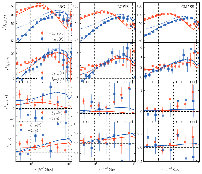
Figure 1: Monopole and quadrupole correlation functions of SDSS galaxies in redshift space, $\xi_{gg,\ell}^{s}$, $\xi_{g+,\ell}^{s}$, $\xi_{+,\ell}^{s}$, and $\xi_{-,\ell}^{s}$ from top to bottom panels. The results for LRG, LOWZ, and CMASS samples are shown from the left to right panels, respectively. The error bars are estimated from jackknife resampling. The solid curves are the best-fit nonlinear alignment and RSD models jointly fitted for these four statistics, where the data points enclosed by the vertical lines are used. The dotted curves are the linear predictions as references.

3 Measurement of correlation functions

In this section, we measure the redshift-space correlation functions of galaxy density and IA from the SDSS samples, and estimate their covariance matrix.

As a conventional clustering analysis, we use a galaxy autocorrelation (GG) function in redshift space, $\xi_{gg}^{s}(\boldsymbol{r})=\left\langle\delta_{g}^{s}(\boldsymbol{x}_{1})\delta_{g}^{s}(\boldsymbol{x}_{2})\right\rangle$, where superscript $s$ denotes the quantity defined in redshift space, $\boldsymbol{r}=\boldsymbol{x}_{2}-\boldsymbol{x}_{1}$, and $\delta_{g}^{s}(\boldsymbol{x})$ is the galaxy number density fluctuation. We adopt the Landy & Szalay (1993) estimator to measure it,

$$\xi_{gg}^{s}(\boldsymbol{r})=\frac{(D-R)^{2}}{RR}=\frac{DD-2DR+RR}{RR},$$ (6)

where $DD$, $RR$, and $DR$ are the normalized counts of galaxy–galaxy, random–random, and galaxy–random pairs, respectively. We then obtain the multipole moments,

$$\xi_{gg,\ell}^{s}(r)=(2\ell+1)\int^{1}_{0}d\mu~{}\xi_{gg}^{s}(r,\mu_{\boldsymbol{r}}){\cal L}_{\ell}(\mu_{\boldsymbol{r}}),$$ (7)

where $r=|\boldsymbol{r}|$, $\mu_{\boldsymbol{r}}$ is the direction cosine between the line of sight and $\boldsymbol{r}$, and ${\cal L}_{\ell}$ is the $\ell$th-order Legendre polynomials. To obtain the multipoles via Eq. (7), we estimate $\xi_{gg}^{s}(r,\mu_{\boldsymbol{r}})$ with the angular bin size of $\Delta\mu_{\boldsymbol{r}}=0.1$ in Eq. (6) and take the sum over $\mu_{\boldsymbol{r}}$.

The first row of Figure 1 shows multipole moments of the GG correlation functions. The first, second, and third columns show the results from the LRG, LOWZ, and CMASS samples, respectively. Since the hexadecapole is noisy, we analyze only the monopole and quadrupole moments (Kaiser, 1987). These correlation functions have been measured in various previous works (e.g., Samushia et al., 2012; Alam et al., 2017) and our measurements are consistent with theirs.

Next, we introduce intrinsic alignment statistics, which are density-weighted quantities. The galaxy position–intrinsic ellipticity (GI) correlation, $\xi_{g+}^{s}$, and intrinsic ellipticity–ellipticity (II) correlations, $\xi_{+}^{s}$ and $\xi_{-}^{s}$, are defined by

$$\xi_{X}^{s}(\boldsymbol{r})=\left\langle\left[1+\delta_{g}(\boldsymbol{x}_{1})\right]\left[1+\delta_{g}(\boldsymbol{x}_{2})\right]W_{X}(\boldsymbol{x}_{1},\boldsymbol{x}_{2})\right\rangle,$$ (8)

where $W_{g+}(\boldsymbol{x}_{1},\boldsymbol{x}_{2})=\gamma_{+}(\boldsymbol{x}_{2})$ and $W_{\pm}(\boldsymbol{x}_{1},\boldsymbol{x}_{2})=\gamma_{+}(\boldsymbol{x}_{1})\gamma_{+}(\boldsymbol{x}_{2})\pm\gamma_{\times}(\boldsymbol{x}_{1})\gamma_{\times}(\boldsymbol{x}_{2})$. For the II correlations, we label $\xi_{+}^{s}$ and $\xi_{-}^{s}$ individually as II$(+)$ and II($-$) correlations, respectively. The GI correlation function is estimated as (Mandelbaum et al., 2006),

$$\xi_{g+}(\boldsymbol{r})=\frac{S_{+}(D-R)}{RR}=\frac{S_{+}D-S_{+}R}{RR}\ ,$$ (9)

where $S_{+}D$ is the sum over all pairs with separation $\boldsymbol{r}$ of the $+$ component of the ellipticity, $S_{+}D=\sum_{i\neq j|\boldsymbol{r}}{\gamma_{+}(j|i)}$, with $\gamma_{+}(j|i)$ being the ellipticity of galaxy $j$ measured relative to the direction to galaxy $i$, and $S_{+}R$ is defined similarly. The II correlation functions are estimated as

$$\xi_{\pm}(\boldsymbol{r})=\frac{S_{+}S_{+}\pm S_{\times}S_{\times}}{RR}\ ,$$ (10)

where $S_{+}S_{+}=\sum_{i\neq j|\boldsymbol{r}}{\gamma_{+}(j|i)\gamma_{+}(i|j)}$ and similarly for $S_{\times}S_{\times}$. Finally, multipole moments for the IA correlations, $\xi_{g+,\ell}^{s}$ and $\xi_{\pm,\ell}^{s}$, are obtained via the same equation as Equation (7). Again, since the hexadecapole is noisy, we analyze only the $\ell=0$ and $\ell=2$ moments.

The second, third, and bottom rows of Figure 1 respectively present redshift-space multipole moments of the GI, II($+$) and II($-$) correlation functions. Both the monopole and quadrupole of the GI correlation are clearly detected in all the three samples. Particularly, LRG are the brightest galaxy sample and shows the strongest signal because IA has a strong luminosity dependence. Though LOWZ has a redshift range similar with LRG, it targets fainter galaxies and thus has higher number density. Therefore, the LOWZ sample shows lower GI amplitude, confirming the earlier detection by Singh & Mandelbaum (2016). We find even a lower GI signal in the CMASS sample. The monopole of the II correlation is clearly detected for the LRG sample, as in Okumura et al. (2009), while the newly measured quadrupole is noisier and consistent with zero. Those for the LOWZ and CMASS samples have much lower amplitude, and are somewhat consistent with zero. Furthermore, their shapes are determined by the adaptive moment and have nonzero correlation due to the PSF at $r>30\,h^{-1}\,{\rm Mpc}$ (Singh & Mandelbaum, 2016).

We estimate the covariance matrix for the measured correlation functions, ${\rm C}_{ij}^{X_{\ell}X^{\prime}_{\ell^{\prime}}}\equiv{\rm C}\left[\xi_{X,\ell}(r_{i}),\xi_{X^{\prime},\ell^{\prime}}(r_{j})\right]$, with $X=\{gg,g+,+,-\}$ and $\ell=\{0,2\}$, using the jackknife resampling method. While jackknife is not an unbiased error estimator, it provides reliable error bars for the statistics whose error is dominated by the shape noise (Mandelbaum et al., 2006). The error bars shown in Figure 1 are the square root of the diagonal components of the covariance matrix.

4 Theoretical prediction

Here we present theoretical models to interpret the measured correlation functions. Since theoretical models are naturally provided in Fourier space, we first present models for the power spectra, $P_{X}^{s}$, perform the Fourier transform,

$$\xi_{X}^{s}(\boldsymbol{r})=\int\frac{d^{3}\boldsymbol{k}}{(2\pi)^{3}}P_{X}^{s}(\boldsymbol{k})e^{i\boldsymbol{k}\cdot\boldsymbol{r}},$$ (11)

where $X=\{gg,g+,+,-\}$, and obtain the multipole moments $\xi_{X,\ell}^{s}$ via Equation (7).

4.1 Galaxy correlations

For the galaxy power spectrum, we adopt nonlinear redshift-space distortion (RSD) model proposed by (Scoccimarro, 2004; Taruya et al., 2010),

$$P_{gg}^{s}(\boldsymbol{k})=\left[b^{2}P_{\delta\delta}(k)+2bf\mu_{\boldsymbol{k}}^{2}P_{\delta\Theta}\right. (k)$$

$$\left.+f^{2}\mu_{\boldsymbol{k}}^{4}P_{\Theta\Theta}(k)\right] D_{\rm FoG}^{2}(k\mu_{\boldsymbol{k}}\sigma_{v}),$$ (12)

where $k=|\boldsymbol{k}|$, $\mu_{\boldsymbol{k}}$ is the direction cosine between the observer’s line of sight and the wavevector $\boldsymbol{k}$, and $b$ the galaxy bias. The quantities $P_{\delta\delta}$ and $P_{\Theta\Theta}$ are the nonlinear autopower spectrum of density and velocity fields, respectively, and $P_{\delta\Theta}$ is the their cross-power spectrum. We adopt the revised Halofit model to compute $P_{\delta\delta}$ (Takahashi et al., 2012), and then $P_{\delta\Theta}$ and $P_{\Theta\Theta}$ are computed using the fitting formulae derived by Hahn et al. (2015). The function $D_{\rm FoG}$ is a damping function due to the Finger-of-God (FoG) effect characterized by the nonlinear velocity dispersion parameter $\sigma_{v}$. We adopt a simple Gaussian function, $D_{\rm FoG}(k\mu_{\boldsymbol{k}}\sigma_{v})=\exp{\left(-k^{2}\mu_{\boldsymbol{k}}^{2}\sigma_{v}^{2}/2\right)}$. With this Gaussian function, the nonlinear multipoles are expressed analytically by a simple Hankel transform (Taruya et al., 2009). In the linear-theory limit, $P_{\delta\delta}=P_{\delta\Theta}=P_{\Theta\Theta}$ and $D_{\rm FoG}=1$, and hence Equation (12) converges to the original Kaiser formula. Since $P_{\delta\delta}$, $P_{\delta\Theta}$ and $P_{\Theta\Theta}$ are proportional to the square of the normalization parameter of the density fluctuation, $\sigma_{8}^{2}(z)$, free parameters for this model are ${\boldsymbol{\theta}}=(b\sigma_{8},f\sigma_{8},\sigma_{v})$.

4.2 Intrinsic alignment correlations

To quantify the cosmological information encoded in the IA statistics, we consider the LA model, which assumes a linear relation between the intrinsic ellipticity and tidal field (Catelan et al., 2001). In Fourier space, the ellipticity projected along the line of sight ($z$-axis) is given by

$$\left(\begin{array}[]{c}\gamma_{+}\\ \gamma_{\times}\end{array}\right)(\boldsymbol{k})=b_{K}\left(\begin{array}[]{c}(k_{x}^{2}-k_{y}^{2})/k^{2}\\ 2k_{x}k_{y}/k^{2}\end{array}\right)\delta_{m}(\boldsymbol{k}),$$ (17)

where $b_{K}$ represents the redshift-dependent coefficient of the intrinsic alignments, which we refer to as the shape bias. We adopt the nonlinear alignment (NLA) model, which replaces the linear matter density field $\delta_{m}$ by the nonlinear one (Bridle & King, 2007). Furthermore, the redshift-space shape field is multiplied by the damping function due to the FoG effect.

Adopting also the nonlinear RSD model in Equation (12), the GI and II power spectra are expressed as

$$P_{g+}^{s}(\boldsymbol{k}) =b_{K}k^{-2}(k_{x}^{2}-k_{y}^{2})\left\{bP_{\delta\delta}(k)+f\mu_{\boldsymbol{k}}^{2}P_{\delta\theta}(k)\right\}$$

$$\qquad\qquad\qquad\qquad\qquad\times D_{\rm FoG}^{2}(k\mu_{\boldsymbol{k}}\sigma_{v}),$$ (18)

$$P_{\pm}^{s}(\boldsymbol{k}) =b_{K}^{2}k^{-4}\left[(k_{x}^{2}-k_{y}^{2})^{2}\pm(2k_{x}k_{y})^{2}\right]P_{\delta\delta}(k)$$

$$\qquad\qquad\qquad\qquad\qquad\times D_{\rm FoG}^{2}(k\mu_{\boldsymbol{k}}\sigma_{v})~{}.$$ (19)

Note that Singh et al. (2015) showed that the shape field is insensitive to RSD. While it is true in the linear RSD model, the FoG effect comes into IA power spectra in the same way as the GG spectrum because it is caused purely by a coordinate transform from real to redshift space (T. Okumura et al. 2023, in preparation).

Similarly to $\xi_{gg,\ell}^{s}$, multipole moments of the IA correlations, $\xi_{g+,\ell}^{s}$ and $\xi_{\pm,\ell}^{s}$, can be expressed by a Hankel transform. Since correlation functions of the projected shape are naturally expressed by the associated Legendre polynomial basis (Kurita & Takada, 2022), the nonlinear model of $\xi_{g+,\ell}^{s}$ and $\xi_{-,\ell}^{s}$ involving the FoG factor produces infinite series for each Legendre multipole. We computed the expansion up to the 12th order and confirmed the convergence of the formula. The nonlinear model of $\xi_{+,\ell}^{s}$ has a form similar with $\xi_{gg,\ell}^{s}$. We have four free parameters for the IA statistics, ${{\boldsymbol{\theta}}}=(b\sigma_{8},b_{K}\sigma_{8},f\sigma_{8},\sigma_{v})$. Taking the linear-theory limit of the GI and II correlation functions, namely $\sigma_{v}\to 0$ limit in Equations (18) and (19), leads to the formulas presented in Okumura & Taruya (2020). We will present the full expressions of IA statistics with the Gaussian damping factor in our upcoming paper.

5 Constraints on growth rate

We perform the likelihood analysis and constrain the growth rate parameter $f\sigma_{8}$ from the three SDSS galaxy samples. Particularly, we show how well the constraints are improved by combining IA statistics with the conventional galaxy clustering statistics. We compare the measured statistics, $\xi_{X,\ell}^{s}$, where $X=\{gg,g+,+,-\}$ and $\ell=\{0,2\}$, to the corresponding predictions. The $\chi^{2}$ statistic is given by

$$\chi^{2}({\boldsymbol{\theta}})=\sum_{i,j,\ell,\ell^{\prime},X,X^{\prime}}{\Delta_{i}^{X_{\ell}}\left({\bf C}^{-1}\right)_{ij}^{X_{\ell}X^{\prime}_{\ell^{\prime}}}\Delta_{j}^{X^{\prime}_{\ell^{\prime}}}},$$ (20)

where $\Delta_{i}^{X_{\ell}}=\xi_{X,\ell}^{s,{\rm obs}}(r_{i})-\xi_{X,\ell}^{s,{\rm th}}(r_{i};{\boldsymbol{\theta}})$ is the difference between the observed correlation function and theoretical prediction with ${\boldsymbol{\theta}}$ being a parameter set to be constrained. The analysis is performed over the scales adopted, $r_{\rm min}\leq r_{i}\leq r_{\rm max}$. Since the jackknife method underestimates the covariance at large scales, we set the maximum separation $r_{\rm max}=100\,h^{-1}\,{\rm Mpc}$. Moreover, as described in Sec. 2, the II correlation functions of LOWZ and CMASS are affected by the residual PSF at $r>30\,h^{-1}\,{\rm Mpc}$ (Singh & Mandelbaum, 2016). We thus set $r_{\rm max}=25\,h^{-1}\,{\rm Mpc}$ for the II correlations of these samples. In Appendix A, we investigate how our constraints change with $r_{\rm min}$, and we adopt $r_{\rm min}=10\,h^{-1}\,{\rm Mpc}$. In Appendix B, we provide further argument that our cosmological constraints are not biased by the effect of the uncorrected PSF. For the clustering-only analysis, the covariance is a $20\times 20$ matrix, while for the full analysis of clustering and IA, it is a $60\times 60$ matrix for LRG and $48\times 48$ for LOWZ and CMASS. The data points used for the analysis are enclosed by the vertical lines in Figure 1.

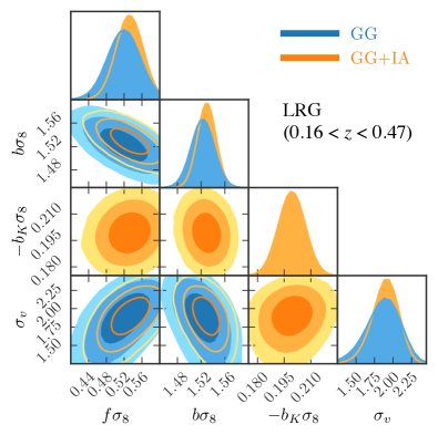
Figure 2: Constraints on $(f\sigma_{8},b\sigma_{8},b_{K}\sigma_{8},\sigma_{v})$ obtained from clustering-only analysis and combined analysis of clustering and IA, determined by the correlation functions of LRG sample at $10\leq r\leq 100\,h^{-1}\,{\rm Mpc}$. The contours show the $68\%,95\%$, and $99\%$ C. L. from inward.

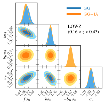
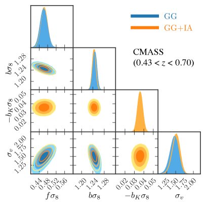
Figure 3: Same as Figure 2, but for LOWZ (top) and CMASS (bottom) samples. For these samples, the II correlations only at $10\leq r\leq 25\,h^{-1}\,{\rm Mpc}$ are used, and the GG and GI correlations at $10\leq r\leq 100\,h^{-1}\,{\rm Mpc}$ are used.

Figure 2 shows the parameter constraints obtained from the LRG sample. The blue and orange contours are results with the clustering-only analysis and its combination with IA statistics, respectively. For the clustering-only analysis, after marginalizing over $b\sigma_{8}$ and $\sigma_{v}$, we obtain the constraint as $f\sigma_{8}=0.5196^{+0.0352}_{-0.0354}$ ($68\%$ confidence level). For the combined analysis of clustering and IA, we obtain $f\sigma_{8}=0.5322^{+0.0293}_{-0.0291}$ by further marginalizing over the shape bias parameter $b_{K}$. Namely, the constraint on $f\sigma_{8}$ is improved by $19\%$ by adding the IA statistics. Note that, as we set $q=0$ in Equation (5), the definition of $b_{K}$ here is different from literature and one cannot directly compare the values.

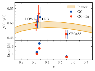
Figure 4: Upper panel: Constraints on growth rate $f(z)\sigma_{8}(z)$ from three SDSS galaxy samples compared to the best-fitting $\Lambda$CDM model from the Planck experiment. We adopt $r_{\rm min}=10\,h^{-1}\,{\rm Mpc}$. Lower panel: $1\sigma$ error of the growth rate constraints, $\Delta(f\sigma_{8})/f\sigma_{8}$.

The left and right panels of Figure 3 show results similar to Figure 2 but for LOWZ and CMASS, respectively. Using LOWZ, we obtain $f\sigma_{8}=0.5043^{+0.0226}_{-0.0229}$ (GG only), and $f\sigma_{8}=0.4937^{+0.0201}_{-0.0201}$ (GG$+$IA). The LOWZ is a denser sample than the LRG by targeting fainter galaxies, and thus, even the galaxy clustering alone puts tighter constraints. However, combining the IA statistics, LRG provides almost as a strong constraint as LOWZ. CMASS is also a fainter population at higher redshift, $0.43<z<0.70$. With the GG-only analysis, we obtain $f\sigma_{8}=0.4614^{+0.0156}_{-0.0154}$, and with the GG+IA analysis, $f\sigma_{8}=0.4628^{+0.0149}_{-0.0151}$. Our analysis of these three galaxy samples demonstrates that the contribution of IA to cosmological constraints can be enhanced by adopting an optimal weighting to brighter galaxies (Seljak et al., 2009). Exploring such an optimization is our future work.

The best-fit nonlinear models jointly fitted for the clustering and IA statistics are shown by the solid curves in Figure 1. Reduced $\chi^{2}$ values obtained for LRG, LOWZ, and CMASS samples are $\chi^{2}/\nu=1.85,1.14$, and $2.42$, respectively, where $\nu$ is the degree of freedom, $\nu=56$ for LRG and $\nu=44$ for LOWZ and CMASS. The large $\chi^{2}$ value for the CMASS sample is due to small error bars in the GG correlation. If we adopt $r_{\rm min}=15\,h^{-1}\,{\rm Mpc}$, the minimum $\chi^{2}$ is reduced to $\chi^{2}/\nu=1.68$. Accordingly, the best-fitting value of $f\sigma_{8}$ is shifted (see Figure 5 in Appendix A).

Finally, Figure 4 summarizes the constraints on $f\sigma_{8}$ from the three galaxy samples we considered. As shown in the lower panel, the constraint gets tighter by adding IA statistics to the galaxy clustering statistics. Overall, the derived results are consistent with the prediction of $\Lambda$CDM determined from the Planck satellite experiment (Planck Collaboration et al., 2020). It indicates that combining IA and clustering statistics enables us to obtain robust and tight constraints.

6 conclusions

We have presented the first cosmological constraints using IA of the SDSS galaxies. We have measured the redshift-space GI and II correlation functions of LRG, LOWZ, and CMASS galaxy samples. By comparing them with the models of nonlinear alignment and RSD effects, we have constrained the growth rate of the density perturbation, $f(z)\sigma_{8}(z)$. We found that combining IA with clustering enhances the growth rate constraint by $\sim 19\%$ compared to the clustering-only analysis for the LRG sample. This improved constraint on $f\sigma_{8}$ is only slightly worse than that obtained from the LOWZ, which is a much denser sample by targeting fainter galaxies. This indicates a potential that the contribution of the IA statistics can be further enhanced by adopting an optimal weighting to brighter galaxies.

In this work we considered only the dynamical constraint via RSD. However, baryon acoustic oscillations (BAOs) observed in the galaxy distributions (Eisenstein et al., 2005) were shown to be also encoded in galaxy IA statistics and thus useful to tighten geometric constraints (Chisari & Dvorkin, 2013; Okumura et al., 2019). The cosmological analysis of IA simultaneously using RSD and BAO will be shown in our future work.

The benefits of using IA can be further enhanced by improving the model. In this paper we worked with a simple extension of the NLA model to include partly the FoG effect (T. Okumura et al. 2023, in preparation). However, more sophisticated nonlinear models of IA statistics have been proposed recently (Blazek et al., 2019; Vlah et al., 2020; Akitsu et al., 2021; Matsubara, 2022). These models enable us to use the measured IA correlation functions down to smaller scales, which will enhance the science return from IA of galaxies.

Appendix A Scale dependence of parameter constraints

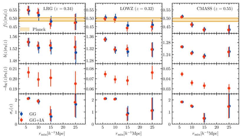
Figure 5: Constraints on model parameters as a function of the minimum separation, $r_{\rm min}$, obtained from clustering-only analysis and combined analysis of clustering and IA for LRG (left), LOWZ (middle) and CMASS (right) samples. We show the results for $f\sigma_{8}$, $b\sigma_{8}$, $b_{K}\sigma_{8}$, and $\sigma_{v}$ from the top to bottom rows. Theoretical prediction with 68% C. L. based on the Planck experiment is shown as the yellow regions in the top row.

In this appendix, we examine how cosmological constraints vary with the scales used in the likelihood analysis. It is important because the growth rate constraint is prone to have scale-dependence due to various nonlinear effects (e.g., Okumura & Jing, 2011). The left column of Figure 5 shows the constraints on parameters for the LRG sample as a function of the minimum separation $r_{\rm min}$ after other three are marginalized over. The constraint on $f\sigma_{8}$ with the clustering-only analysis shows a strong scale dependence, with the same trend as the simulation result (Okumura & Jing, 2011). The combined analysis of clustering and IA shows the same tendency. Since the combined analysis with the scale cut of $r_{\rm min}=10\,h^{-1}\,{\rm Mpc}$ gives the best-fitting value of $f\sigma_{8}$ expected at the large scale limit ($25<r<100~{}[\,h^{-1}\,{\rm Mpc}\ ]$), we present it as the main result of this paper. The middle and right columns of Figure 5 show the scale dependence of parameter constraints obtained from the LOWZ and CMASS samples, respectively. The overall tendency of the constraints on $f\sigma_{8}$ is similar to that for the LRG sample. For consistency, we also adopt $r_{\rm min}=10\,h^{-1}\,{\rm Mpc}$ for the analysis of the LOWZ and CMASS samples. However, as mentioned in Sec. 5, small error bars in the GG correlation of the CMASS sample result in the large $\chi^{2}$ value when we choose $r_{\rm min}=10\,h^{-1}\,{\rm Mpc}$ ($\chi^{2}/\nu=2.42$). If we adopt $r_{\rm min}=15\,h^{-1}\,{\rm Mpc}$, the minimum $\chi^{2}$ is reduced to $\chi^{2}/\nu=1.68$. Accordingly, the best-fitting value of $f\sigma_{8}$ is shifted.

Appendix B Effect of PSF on parameter constraints

As described in Sec. 2, the ellipticity of LRG is defined by the isophote of the light profile while that of LOWZ and CMASS galaxies is by the adaptive moment. Singh & Mandelbaum (2016) constructed the shape catalog for the LRG and LOWZ samples using a re-Gaussianization technique, which is based on the adaptive moment but involves additional steps to correct for non-Gaussianity of both the PSF and galaxy surface brightness profile (Hirata & Seljak, 2003). Utilizing it, Singh & Mandelbaum (2016) found that while the isophotal shape is not corrected for the PSF, the measured IA statistics are not so biased because the method uses the outer shape of the galaxies. Eventually, the uncorrected PSF affects only the amplitude of the measured IA statistics, not the shape, which has already been confirmed by our earlier work (Okumura et al., 2009). Furthermore, Okumura & Jing (2009) showed that the amplitude of IA, namely the shape bias $b_{K}$, determined by the GI and II correlations is fully consistent with each other. Therefore, while the constraint on $b_{K}$ can be different from the true value, that on the growth rate $f$ is not expected to be biased after $b_{K}$ is marginalized over. While the adaptive moment corrects for the PSF in the ellipticity, it results in a small bias (Hirata & Seljak, 2003). However, it is a constant bias, and thus it affects the amplitude of $b_{K}$, similarly to the isophotal shape definition but the effect is smaller. To be conservative, we exclude the II correlation at $r>25\,h^{-1}\,{\rm Mpc}$ which is affected if we adopt the less accurate, de Vaucouleurs model fit(Singh & Mandelbaum, 2016). Namely, the constraints from LOWZ and CMASS samples on $f\sigma_{8}$ with $r_{\rm min}=25\,h^{-1}\,{\rm Mpc}$ in Fig. 5 do not use the data of the II correlation., Nevertheless, the constraints are almost equivalent to those with $r_{\rm min}=15\,h^{-1}\,{\rm Mpc}$. It implies that the bias which arises from the uncorrected PSF is negligible for the shape definition of LOWZ and CMASS galaxies.

For all the three galaxy samples, constrained values of the model parameters do not change significantly by combining the IA statistics with the clustering statistics but shrink the error bars. It demonstrates that systematic effects associated with the shape measurement do not contribute to biases in the parameter constraints. More concrete discussion of uncorrected PSF effects on cosmological constraints requires the construction of shape catalogs in which the systematic effects are fully corrected for (Hirata & Seljak, 2003; Singh & Mandelbaum, 2016). It will be investigated in future work.

References

- Akitsu et al. (2021) Akitsu, K., Li, Y., & Okumura, T. 2021, J. Cosmology Astropart. Phys, 2021, 041
- Alam et al. (2017) Alam, S., Ata, M., Bailey, S., et al. 2017, MNRAS, 470, 2617
- Bernstein & Jarvis (2002) Bernstein, G. M., & Jarvis, M. 2002, AJ, 123, 583
- Blazek et al. (2019) Blazek, J. A., MacCrann, N., Troxel, M. A., & Fang, X. 2019, Phys. Rev. D, 100, 103506
- Bridle & King (2007) Bridle, S., & King, L. 2007, New Journal of Physics, 9, 444
- Catelan et al. (2001) Catelan, P., Kamionkowski, M., & Blandford, R. D. 2001, MNRAS, 320, L7
- Chisari & Dvorkin (2013) Chisari, N. E., & Dvorkin, C. 2013, J. Cosmology Astropart. Phys, 12, 029
- Chuang et al. (2022) Chuang, Y.-T., Okumura, T., & Shirasaki, M. 2022, MNRAS, 515, 4464
- Croft & Metzler (2000) Croft, R. A. C., & Metzler, C. A. 2000, ApJ, 545, 561
- DESI Collaboration et al. (2016) DESI Collaboration, Aghamousa, A., Aguilar, J., et al. 2016, arXiv e-prints, arXiv:1611.00036
- Eisenstein et al. (2001) Eisenstein, D. J., Annis, J., Gunn, J. E., et al. 2001, AJ, 122, 2267
- Eisenstein et al. (2005) Eisenstein, D. J., Zehavi, I., Hogg, D. W., et al. 2005, ApJ, 633, 560
- Hahn et al. (2015) Hahn, O., Angulo, R. E., & Abel, T. 2015, MNRAS, 454, 3920
- Heavens et al. (2000) Heavens, A., Refregier, A., & Heymans, C. 2000, MNRAS, 319, 649
- Hikage et al. (2019) Hikage, C., Oguri, M., Hamana, T., et al. 2019, PASJ, 71, 43
- Hirata & Seljak (2003) Hirata, C., & Seljak, U. 2003, MNRAS, 343, 459
- Hirata & Seljak (2004) Hirata, C. M., & Seljak, U. 2004, Phys. Rev. D, 70, 063526
- Joachimi et al. (2011) Joachimi, B., Mandelbaum, R., Abdalla, F. B., & Bridle, S. L. 2011, A&A, 527, A26
- Kaiser (1987) Kaiser, N. 1987, MNRAS, 227, 1
- Kurita & Takada (2022) Kurita, T., & Takada, M. 2022, Phys. Rev. D, 105, 123501
- Kurita et al. (2021) Kurita, T., Takada, M., Nishimichi, T., et al. 2021, MNRAS, 501, 833
- Landy & Szalay (1993) Landy, S. D., & Szalay, A. S. 1993, ApJ, 412, 64
- Lee et al. (2023) Lee, J., Ryu, S., & Baldi, M. 2023, ApJ, 945, 15
- Li et al. (2013) Li, C., Jing, Y. P., Faltenbacher, A., & Wang, J. 2013, ApJ, 770, L12
- Mandelbaum et al. (2006) Mandelbaum, R., Hirata, C. M., Ishak, M., Seljak, U., & Brinkmann, J. 2006, MNRAS, 367, 611
- Matsubara (2022) Matsubara, T. 2022, arXiv e-prints, arXiv:2210.10435
- Okumura & Jing (2009) Okumura, T., & Jing, Y. P. 2009, ApJ, 694, L83
- Okumura & Jing (2011) —. 2011, ApJ, 726, 5
- Okumura et al. (2009) Okumura, T., Jing, Y. P., & Li, C. 2009, ApJ, 694, 214
- Okumura & Taruya (2020) Okumura, T., & Taruya, A. 2020, MNRAS, 493, L124
- Okumura & Taruya (2022) —. 2022, Phys. Rev. D, 106, 043523
- Okumura et al. (2019) Okumura, T., Taruya, A., & Nishimichi, T. 2019, Phys. Rev. D, 100, 103507
- Okumura et al. (2020) —. 2020, MNRAS, 494, 694
- Planck Collaboration et al. (2020) Planck Collaboration, Aghanim, N., Akrami, Y., et al. 2020, A&A, 641, A6
- Reid et al. (2016) Reid, B., Ho, S., Padmanabhan, N., et al. 2016, MNRAS, 455, 1553
- Saga et al. (2023) Saga, S., Okumura, T., Taruya, A., & Inoue, T. 2023, MNRAS, 518, 4976
- Samushia et al. (2012) Samushia, L., Percival, W. J., & Raccanelli, A. 2012, MNRAS, 420, 2102
- Schmidt et al. (2015) Schmidt, F., Chisari, N. E., & Dvorkin, C. 2015, J. Cosmology Astropart. Phys, 10, 032
- Scoccimarro (2004) Scoccimarro, R. 2004, Phys. Rev. D, 70, 083007
- Seljak et al. (2009) Seljak, U., Hamaus, N., & Desjacques, V. 2009, Physical Review Letters, 103, 091303
- Singh & Mandelbaum (2016) Singh, S., & Mandelbaum, R. 2016, MNRAS, 457, 2301
- Singh et al. (2015) Singh, S., Mandelbaum, R., & More, S. 2015, MNRAS, 450, 2195
- Takada et al. (2014) Takada, M., Ellis, R. S., Chiba, M., et al. 2014, PASJ, 66, 1
- Takahashi et al. (2012) Takahashi, R., Sato, M., Nishimichi, T., Taruya, A., & Oguri, M. 2012, ApJ, 761, 152
- Taruya et al. (2010) Taruya, A., Nishimichi, T., & Saito, S. 2010, Phys. Rev. D, 82, 063522
- Taruya et al. (2009) Taruya, A., Nishimichi, T., Saito, S., & Hiramatsu, T. 2009, Phys. Rev. D, 80, 123503
- Taruya & Okumura (2020) Taruya, A., & Okumura, T. 2020, ApJ, 891, L42
- Tonegawa & Okumura (2022) Tonegawa, M., & Okumura, T. 2022, ApJ, 924, L3
- Vlah et al. (2020) Vlah, Z., Chisari, N. E., & Schmidt, F. 2020, J. Cosmology Astropart. Phys, 1, 025
- Zwetsloot & Chisari (2022) Zwetsloot, K., & Chisari, N. E. 2022, MNRAS, 516, 787