An Efficient Approach for Discovering Graph Entity Dependencies (GEDs)

Abstract

Graph entity dependencies (GEDs) are novel graph constraints, unifying keys and functional dependencies, for property graphs. They have been found useful in many real-world data quality and data management tasks, including fact checking on social media networks and entity resolution. In this paper, we study the discovery problem of GEDs – finding a minimal cover of valid GEDs in a given graph data. We formalise the problem, and propose an effective and efficient approach to overcome major bottlenecks in GED discovery. In particular, we leverage existing graph partitioning algorithms to enable fast GED-scope discovery, and employ effective pruning strategies over the prohibitively large space of candidate dependencies. Furthermore, we define an interestingness measure for GEDs based on the minimum description length principle, to score and rank the mined cover set of GEDs. Finally, we demonstrate the scalability and effectiveness of our GED discovery approach through extensive experiments on real-world benchmark graph data sets; and present the usefulness of the discovered rules in different downstream data quality management applications.

[ci]organization=College of Informatics, addressline=Huazhong Agric. University, city=Wuhan, state=Hubei, country=China

[cd]organization=AI & Cyber Futures Institute, addressline=Charles Sturt University, city=Bathurst, state=NSW, country=Australia

[scm]organization=School of Computing & Mathematics, addressline=Charles Sturt University, city=Wagga Wagga, state=NSW, country=Australia

[sc]organization=School of Computer, addressline=Wuhan University, city=Wuhan, state=Hubei, country=China

]Zaiwen.Feng@mail.hzau.edu.cn

A study of the discovery problem of Graph Entity Dependencies (GEDs).

A new and efficient approach for the discovery of GEDs in property graphs.

A minimum description length inspired definition of interestingness of GEDs to rank discovered rules.

A thorough empirical evaluation of the proposed technique, with examples of useful rules (mined) that are relevant in data quality/management applications.

1 Introduction

In recent years, integrity constraints (e.g., keys [1] and functional dependencies (FDs) [2]) have been proposed for property graphs to enable the specification of various data semantics, and tackling of graph data quality and management problems. Graph entity dependencies (GEDs) [4, 5] are new fundamental constraints unifying keys and FDs for property graphs.

A GED $\varphi$ over a graph $G$ is a pair, $\varphi=(Q[\bar{u}],X\to Y)$, specifying the dependency $X\to Y$ over homomorphic matches of the graph pattern $Q[\bar{u}]$ in $G$. Intuitively, since graphs are schemaless, the graph pattern $Q[\bar{u}]$ identifies which the set of entities in $G$ on which the dependency $X\to Y$ should hold. In general, GEDs are capable of expressing and encoding the semantics of relational FDs and conditional FDs (CFDs), as well as subsume other graph integrity constraints (e.g., GKeys [1] and GFDs [2]).

GEDs have numerous real-world data quality and data management applications (cf. [4, 5] for more details). For example, they have been extended and used for: fact checking in social media networks [20], entity resolution in graphs and relations [3, 6, 22], consistency checking [21], knowledge graph generation [51], amongst others.

In this work, motivated by the expressivity and usefulness of GEDs in many downstream applications, we study the problem of automatically learning GEDs from a given property graph. To the best of our knowledge, at the moment, no discovery algorithm exists in the literature for GEDs, albeit discovery solutions have been proposed for graph keys and GFDs in [12] and [16] respectively. However, the GFD mining solutions in [16] mine a special class of GEDs (without any id-literals, using isomorphic matching semantics). Further, [16, 12] considers the discovery of key constraints in RDFs. Thus, the need for effective and efficient techniques for mining rules that capture the full GED semantics still exists.

Discovering data dependencies is an active and long-standing research problem within the database and data mining communities. Indeed, the problem is well-studied for the relational data setting, with volumes of contributions for functional dependencies (FDs) [8, 19, 44, 18] and its numerous extensions (e.g., conditional FDs [7, 26, 24], distance-based FDs [10, 9, 14, 15, 13], etc).

The general goal in data dependency mining is to find an irreducible set (aka. minimal cover set) of valid dependencies (devoid of all implications and redundancies) that hold over the given input data. This is a challenging and often intractable problem for most dependencies, and GEDs are not an exception. In fact, the problem is inherently more challenging for GEDs than it is for other graph constraints (e.g. GFDs and GKeys) and traditional relational dependencies. The reason is three-fold: a) the presence of graph pattern as topological constraints (unseen in relational dependencies); b) the attribute sets of GED dependency have three possible literals (e.g., GFDs have 2, GKeys have 1, CFDs have 2); c) the implication and validation analyses—key tasks in the discovery process—of GEDs are shown NP-complete and co-NP-complete respectively (see [5] for details).

This paper proposes an efficient and effective GED mining solution. We observe that, two major efficiency bottlenecks in mining GEDs are on pattern discovery in large graphs, traversal of the prohibitively large search space of candidate dependencies. Thus, we leverage existing graph partitioning algorithms to surmount the first challenge, and employ several effective pruning rules and strategies to resolve the second.

We summarise our main contributions as follows. 1) We formalise the GED discovery problem (in Section 3). We extend the notions of trivial, reduced, and minimal dependencies for GEDs; and introduce a formal cover set finding problem for GEDs. 2) We develop a new two-phase approach for efficiently finding GEDs in large graphs (Setion 4). The developed solution leverages existing graph partitioning algorithms to mine graph patterns quickly, and find their matches. Further, we design a comprehensive attribute (and entity) dependency discovery architecture with effective candidate generation, search space pruning and validation strategies. Moreover, we introduce a new interestingness score for GEDs, for ranking the discovered rules. 3) We perform extensive experiments on real-world graphs to show that GED discovery can be feasible in large graphs, and demonstrate the effectiveness, scalability and efficiency of our proposed approach (Section 5).

2 Preliminaries

This section presents preliminary concepts and definitions. We use $\mathbf{A,L,C}$ to be denote universal sets of attributes, labels and constants respectively. The definitions of graph, graph pattern, and matches follow those in [4, 5].

Graph. We consider a directed property graph $G=(V,E,L,F_{A})$, where: (1) $V$ is a finite set of nodes; (2) $E$ is a finite set of edges, given by $E\subseteq V\times\mathbf{L}\times V$, in which $(v,l,v^{\prime})$ is an edge from node $v$ to node $v^{\prime}$ with label $l\in\mathbf{L}$; (3) each node $v\in V$ has a special attribute $id$ denoting its identity, and a label $L(v)$ drawn from $\mathbf{L}$; (4) every node $v$, has an associated list $F_{A}(v)=[(A_{1},c_{1}),...,(A_{n},c_{n})]$ of attribute-value pairs, where $c_{i}\in\mathbf{C}$ is a constant, $A_{i}\in\mathbf{A}$ is an attribute of $v$, written as $v.A_{i}=c_{i}$, and $A_{i}\neq A_{j}$ if $i\neq j$.

Graph Pattern. A graph pattern, denoted by $Q[\bar{u}]$, is a directed graph $Q[\bar{u}]=(V_{Q},E_{Q},L_{Q})$, where: (a) $V_{Q}$ and $E_{Q}$ represent the set of pattern nodes and pattern edges respectively; (b) $L_{Q}$ is a label function that assigns a label to each node $v\in V_{Q}$ and each edge $e\in E_{Q}$; and (c) $\bar{u}$ is all the nodes, called (pattern) variables in $V_{Q}$. All labels are drawn from $\mathbf{L}$, including the wildcard “*” as a special label. Two labels $l,l^{\prime}\in\mathbf{L}$ are said to match, denoted $l\asymp l^{\prime}$ iff: (a) $l=l^{\prime}$; or (b) either $l$ or $l^{\prime}$ is “*”.

A match of a graph pattern $Q[\bar{u}]$ in a graph $G$ is a homomorphism $h$ from $Q$ to $G$ such that: (a) for each node $v\in V_{Q}$, $L_{Q}(v)\asymp L(h(v))$; and (b) each edge $e=(v,l,v^{\prime})\in E_{Q}$, there exists an edge $e^{\prime}=(h(v),l^{\prime},h(v^{\prime}))$ in $G$, such that $l\asymp l^{\prime}$. We denote the list of all matches of $Q[\bar{u}]$ in $G$ by $H(\bar{u})$. An example of a graph, graph patterns and their matches are presented below in Example 1.

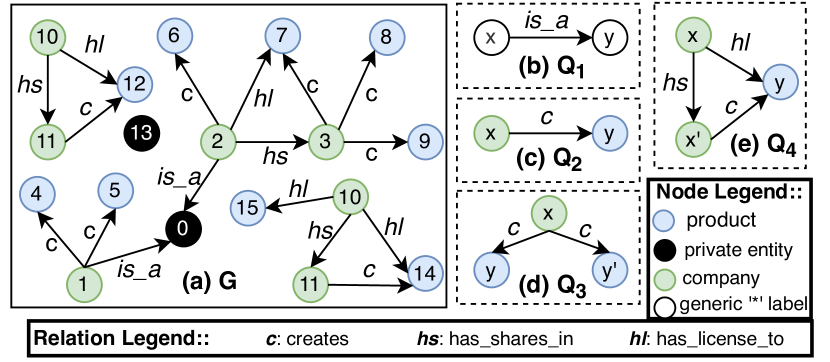
Figure 1: Example: (a) graph; (b)–(d) graph patterns

Example 1 (Graph, Graph Pattern & Matching)

Figure 1(a) depicts a simple graph; and (b)–(e) are examples of four graph patterns. $Q_{1}[x,y]$ describes an “is a” relationship between two generic (“*” labelled) nodes $x$ and $y$. The list of matches of this pattern in the example graph is $H_{1}(x,y)=[\{1,0\},\{2,0\}]$. $Q_{2}[x,y]$ depicts a company node $x$ with a create relation with a product node $y$, its matches in $G:H_{2}(x,y)=[\{1,4\}\{1,5\}\{2,6\},\{3,7\},\{3,8\}$, $\{3,9\},\{11,12\},\{11,14\}]$. $Q_{3}[x,y,y^{\prime}]$ specifies a company node $x$ with a create relation with two product nodes $y,y^{\prime}$. Thus, matches in $G$ are $H_{3}(x,y,y^{\prime})=[\{1,4,5\},\{3,7,8\},\{3,7,9\},\{3,8,9\}]$. $Q_{4}[x,x^{\prime},y]$ describes a company $x$ with a has shares in relation with another company $x^{\prime}$, and a has license to relation with a product $y$ created by $x^{\prime}$. $H_{4}(x,x^{\prime},y)=[\{2,4,7\},\{10,11,12\},\{10$, $11,14\}]$.

Graph Entity Dependencies. A graph entity dependency (GED) [4] $\varphi$ is a pair $(Q[\bar{u}],X\to Y)$, where $Q[\bar{u}]$ is a graph pattern, and $X,Y$ are two (possibly empty) sets of literals in $\bar{u}$. A literal $w$ of $\bar{u}$ is one of the following three constraints: (a) $x.A=c$, (b) $x.A=y.A^{\prime}$, (c) $x.id=y.id$, where $x,y\in\bar{u}$, are pattern variables, $A,A^{\prime}\in\mathbf{A}$, are non-$id$ attributes, and $c\in\mathbf{C}$ is a constant. $Q[\bar{u}]$, and $X\to Y$ are referred to as the pattern/scope and dependency of $\varphi$ respectively.

Given a GED $\varphi=(Q[\bar{u}],X\to Y)$, a match $h(\bar{u})$ of $Q[\bar{u}]$ in $G$ satisfies a literal $w$ of $\bar{u}$, denoted by $h(\bar{u})\models w$, if: (a) when $w$ is $x.A=c$, then the attribute $h(x).A$ exists, and $h(x).A=c$; (b) when $w$ is $x.A=y.A^{\prime}$, then the attributes $h(x).A$ and $h(y).A^{\prime}$ exist and have the same value; (c) when $w$ is $x.id=y.id$, then $h(x).id=h(y).id$.

A match $h(\bar{u})$ satisfies a set $X$ of literals if $h(\bar{u})$ satisfies every literal $w\in X$, (similarly defined for $h(\bar{u})\models Y$). We write $h(\bar{u})\models X\to Y$ if $h(\bar{x})\models X$ implies $h(\bar{x})\models Y$.

A graph $G$ satisfies GED $\varphi$, denoted by $G\models\varphi$, if for all matches $h(\bar{u})$ of $Q[\bar{u}]$ in $G$, $h(\bar{x})\models X\to Y$. A graph, $G$, satisfies a set $\Sigma$ of GEDs, denoted by $G\models\Sigma$, if for all $\varphi\in\Sigma$, $G\models\varphi$.

We illustrate the semantics of GEDs via the sample graph and graph patterns in Figure 1 below.

Example 2 (GEDs)

We define exemplar GEDs over the sample graph in Figure 1(a), using the graph patterns in Figure 1(b)–(e). 1) $\varphi_{1}:(Q_{1}[x,y],y.A=y.A\to x.A=y.A)$ – this GED states that for any match $h(x,y)$ of the pattern $Q_{1}[x,y]$ in $G$ (i.e., $x$ is_a $y$), if the node $h(y)$ has property $A$, then $h(x)$ must have same values as $h(y)$ on $A$. 2) $\varphi_{2}:(Q_{2}[x,y],\emptyset\to y.creator=x.name)$ – for every match $h(x,y)$ of $Q_{2}$ in $G$ (i.e., company $h(x)$ create product $h(y)$), then $h(y.creator)$ and $h(x.name)$ must have the same value. 3) $\varphi_{3}:(Q_{3}[x,y,y^{\prime}],\emptyset\to y.creator=y^{\prime}.creator)$ – this states for any match $h(x,y,y^{\prime})$ in $G$ (i.e., the company $h(x)$ create two products $h(y,y^{\prime})$), then $y,y^{\prime}$ must have same value on their property/attribute $creator$. 4) $\varphi_{4}:(Q_{4}[x,x^{\prime},y],x^{\prime}.country=$ USA$\to x.country=$ USA) – for every match $h(x,x^{\prime},y)$ of $Q_{4}$ in $G$, if $h(x^{\prime}.country)$ is USA, then $h(x.country)$ must also be USA. Note that, $\varphi_{4}$ over $G$ restricts share/license ownership in any USA company to only USA companies.

3 Problem Formulation

Given a property graph $G$, the general GED discovery problem is to find a set $\Sigma$ of GEDs such that $G\models\Sigma$. However, like other dependency discovery problems, such a set can be large and littered with redundancies (cf. [16, 22, 44]). Thus, in line with [16], we are interested in finding a cover set of non-trivial and non-redundant dependencies over persistent graph patterns. In the following, we formally introduce the GEDs of interest, and present our problem definition.

Persistent Graph Patterns. Graph patterns can be seen as “loose schemas” in GEDs [5]. It is therefore crucial to find persistent graph patterns in the input graph data for GED discovery. However, counting the frequency of sub-graphs is a non-trivial task, and can be intractable depending on the adopted count-metric (e.g., harmful overlap [30], and maximum independent sets [29]).

We adopt the minimum image based support (MNI) [45] metric to count the occurrence of a graph pattern in a given graph, due to its anti-monotone and tractability properties.

Let $I=\{i_{1},\cdots,i_{m}\}$ be the set of isomorphisms of a pattern $Q[\bar{u}]$ to a graph $G$. Let $M(v)=\{i_{1}(v),\cdots,i_{m}(v)\}$ be the set containing the (distinct) nodes in $G$ whose functions $i_{1},\cdots,i_{m}$ map a node $v\in V$. The MNI of $Q$ in $G$, denoted by $mni(Q,G)$, is defined as:

$$mni(Q,G)=min\{x\mid x=|M(v)|,\mbox{ }\forall\mbox{ }v\in V\}.$$ (3.1)

We say a graph pattern $Q[\bar{u}]$ is persistent (i.e., frequent) in a graph $G$, if $mni(Q,G)\geq\tau$, where $\tau$ is a user-specified minimum MNI threshold.

Representative Graph Patterns. For many real-world graphs, it is prohibitively inefficient to mine frequent graph patterns with commodity computational resources largely due to their sizes (cf. [31, 32]). To alleviate this performance bottleneck, in our pipeline, we consider graph patterns that are frequent within densely-connected communities within the input graph. We term such graph patterns representative, and adopt the Constant Potts Model (CPM) [35] as the quality function for communities in a graph.

Formally, the CPM of a community $c$ is given by

$$\mathcal{H}=\sum_{c}\left[e_{c}-\gamma\binom{n_{c}}{2}\right]$$ (3.2)

where $e_{c}$ and $n_{c}$ are the number of edges and nodes in $c$ respectively; and $\gamma>0$ is a (user-specified) resolution parameter—higher $\gamma$ leads to more communities, and vice versa. Intuitively, the resolution parameter, $\gamma$, constrains the intra- and inter-community densities to be no less than and no more than the value of $\gamma$ respectively.

Thus, we say a graph pattern $Q[\bar{u}]$ is representative or $(\gamma,\tau)$-frequent if it is $\tau$-frequent within at least one $\gamma$-dense community $c\in G$.

Trivial GEDs. We say a GED $\varphi:(Q[\bar{u}],X\to Y)$ is trivial if: (a) the set of literals in $X$ cannot be satisfied (i.e., $X$ evaluates to false); or (b) $Y$ is derivable from $X$ (i.e., $\forall\mbox{ }w\in Y$, $w$ can be derived from $X$ by transitivity of the equality operator). We consider non-trivial GEDs.

Reduced GEDs. Given two patterns $Q[\bar{u}]=(V_{Q},E_{Q},L_{Q}),Q^{\prime}[\bar{u^{\prime}}]=(V^{\prime}_{Q^{\prime}},E^{\prime}_{Q^{\prime}},L^{\prime}_{Q^{\prime}})$, $Q[\bar{u}]$ is said to reduce $Q^{\prime}[\bar{u^{\prime}}]$, denoted as $Q\ll Q^{\prime}$ if: (a) $V_{Q}\subseteq V^{\prime}_{Q^{\prime}}$, $E_{Q}\subseteq E^{\prime}_{Q^{\prime}}$; or (b) $L_{Q}$ upgrades some labels in $L^{\prime}_{Q^{\prime}}$ to wildcards. That is, $Q$ is a less restrictive topological constraint than $Q^{\prime}$.

Given two GEDs, $\varphi=(Q[\bar{u}],X\to w)$ and $\varphi^{\prime}=(Q^{\prime}[\bar{u^{\prime}}],X^{\prime}\to w^{\prime})$. $\varphi$ is said to reduce $\varphi^{\prime}$, denoted by $\varphi\ll\varphi^{\prime}$, if: (a) $Q\ll Q^{\prime}$; and (b) $X\subseteq X^{\prime}$ and $w=w^{\prime}$.

Thus, we say a GED $\varphi$ is reduced in a graph $G$ if: (a) $G\models\varphi$; and for any $\varphi^{\prime}$ such that $\varphi^{\prime}\ll\varphi$, $G\not\models\varphi^{\prime}$. We say a GED $\varphi$ is minimal if it is both non-trivial and reduced.

Cover of GEDs. Given a set $\Sigma$ of GEDs such that $G\models\Sigma$. $\Sigma$ is minimal iff: for all $\varphi\in\Sigma$, we have $\Sigma\not\equiv\Sigma\setminus\varphi$. That is, $\Sigma$ contains no redundant GED. We say $\Sigma_{c}$ is a cover of $\Sigma$ on $G$ if: (a) $\Sigma_{c}\subseteq\Sigma$; (b) $\Sigma_{c}\equiv\Sigma$; (c) all $\varphi\in\Sigma_{c}$ are minimal; and (d) $\Sigma_{c}$ is minimal.

We study the following GED discovery problem.

Definition 1 (Discovery of GEDs)

Given a property graph, $G$, and user-specified resolution parameter and MNI thresholds $\gamma,\tau$: find a cover set $\Sigma_{c}$ of all valid minimal GEDs that hold over $(\gamma,\tau)$-frequent graph patterns in $G$.

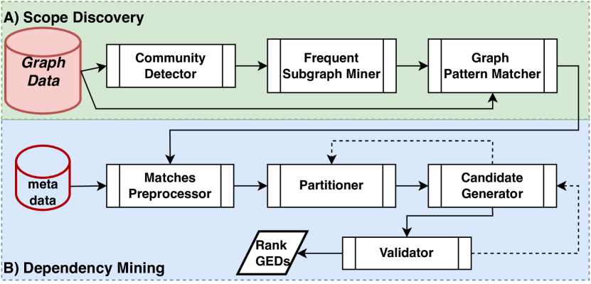
Figure 2: The Overall GED Discovery Pipeline.

4 The Proposed Discovery Approach

This section introduces a new and efficient GED discovery approach. Figure 2 presents the overall pipeline of our solution, consisting of two main components for: (a) finding representative and reduced graph patterns (i.e., “scopes”) and their (homomorphic) matches in the graph; and (b) finding minimal attribute (entity) dependencies that holds over the graph patterns. A snippet of the pseudo-code for the proposed GED discovery process is presented Algorithm 1, requiring two main procedures for the above-mentioned tasks (cf. lines 4 and 5–7 of Algorithm 1 respectively). The required input to the algorithm includes: a property graph, $G$; a user-specified resolution parameter $\gamma$ and minimum MNI threshold $\tau$.

Algorithm 1 DisGEDs

1:A graph, $G$; CPM resolution-parameter, $\gamma$; MNI threshold, $\tau$.

2:A cover set $\Sigma_{c}$ of GEDs (with $\tau$-frequent graph patterns) in $G$

3:$\Sigma_{c}:=\emptyset;\Sigma:=\emptyset;\mathcal{S}:=\emptyset$

4:$\mathcal{S}\leftarrow mineScopes(G,\gamma,\tau)$$\triangleright$ find graph patterns & their matches

5:for each $(Q_{i},H(Q_{i},G))\in\mathcal{S}$ do$\triangleright$ mine minimal GEDs

6:     $\Sigma_{i}\leftarrow mineDependencies(Q_{i},H(Q_{i},G))$

7:     $\Sigma\leftarrow\Sigma\cup\Sigma_{i}$

8:$\Sigma_{c}\leftarrow findCover(\Sigma)$$\triangleright$ remove all transitively implied GEDs

9:return $\Sigma_{c}$

4.1 Graph Pattern Discovery & Matching

The first task in the discovery process is finding representative graph patterns, and their matches in the given graph. We present a three-phase process for the task, viz.: (i) detection of dense communities within the input graph; (ii) mining frequent graph patterns in communities; and (iii) finding matches of the discovered (and reduced) graph patterns in the input graph.

Procedure 1, mineScopes($G,\gamma,\tau$), presents the pseudo-code for this task (with workflow depicted in Figure 2 A).

4.1.1 Dense communities detection

The first step in our approach is straightforward: division of the input

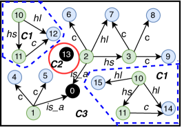
Figure 3: $0.01$-dense communities in example graph $G:C1,C2,C3$

graph $G$ into multiple dense communities, $\mathcal{C}=\{c_{1},\cdots,c_{k}$}. In particular, we employ the quality function in Equation 3.2 to ensure that the density of each community $c_{i}\in\mathcal{C},(i\in[1,k])$ is no less than $\gamma$. In general, any efficient graph clustering algorithm can be employed for this task; and we adopt the Leiden graph clustering algorithm [37] with the CPM quality function to partition the input graph into $\gamma$-dense communities (cf. line 4 in Procedure 1).

As an example, consider our sample graph in Figure 1 (a). For a resolution value of $\gamma=0.01$, three dense communities are produced as show in Figure 3. This includes: $c_{1}$, portion of the graph enclosed by the dotted blue lines; $c_{2}$, a single node $13$; and $c_{3}$, the remaining graph.

Procedure 1 mineScopes($G,\gamma,\tau$)

1:Graph, $G$; CPM resolution-parameter, $\gamma$; MNI threshold, $\tau$

2:Set $\mathcal{S}=\{(Q_{1},H(Q_{1},G)),\cdots\}$ of reduced patterns $Q_{i}$ and their homomorphic matches $H(Q_{i},G)$ in $G$

3:$\mathcal{C}:=\emptyset;\mathcal{Q}:=\emptyset;\mathcal{S}:=\emptyset;G^{\prime}=\emptyset$

4:$\mathcal{C}\leftarrow{\tt Leiden}(G,\gamma)$$\triangleright$ mine dense communities

5:for $c_{i}\in\mathcal{C}$ do$\triangleright$ mine frequent sup-graph patterns

6:     $\mathcal{Q}_{i}\leftarrow{\tt GraMi}(c_{i},\tau)$

7:     $\mathcal{Q}\leftarrow\mathcal{Q}\cup\mathcal{Q}_{i}$

8:$\mathcal{Q}^{\prime}\leftarrow reduceGraphPatterns(\mathcal{Q})$

9:for $Q\in\mathcal{Q}^{\prime}$ do$\triangleright$ find homomorphic matches

10:     $G^{\prime}\leftarrow{\tt filter}(G,Q)$$\triangleright$ filter $G$ w.r.t. edges/nodes in $Q$

11:     $H(Q,G)\leftarrow{\tt match}(Q,G^{\prime})$

12:     $\mathcal{S}\leftarrow\mathcal{S}\cup(Q,H(Q,G))$

13:return $\mathcal{S}$

4.1.2 Representative Graph Patterns Mining

Next, we take the discovered $\gamma$-dense communities, $\mathcal{C}=\{c_{1},\cdots,c_{k}\}$ as input, and return a set of frequent and reduced graph patterns, using isomorphic matching and the MNI metric (in Equation 3.1) to count patterns occurrences in the communities (cf. lines 5–8 of Procedure 1).

We adapt the GraMi graph patterns mining algorithm [28] to find the set, $\mathcal{Q}$, of all $\tau$-frequent patterns across $c_{1},\cdots,c_{k}$. As will be expected, $\mathcal{Q}$ may contain redundant patterns. Therefore, we designed a simple and effective algorithm, Function 1, to prune all redundancies in $\mathcal{Q}$, and return a set $\mathcal{Q}^{\prime}$ of representative and reduced patterns in $G$ (i.e., there does not exist any pair of patterns $Q,Q^{\prime}\in\mathcal{Q}^{\prime}$ such that $Q\ll Q^{\prime}$ or $Q^{\prime}\ll Q$).

Function 1 $reduceGraphPatterns(\mathcal{Q})$

1:$n\leftarrow|\mathcal{Q}|;\mathcal{Q}^{\prime}:=\emptyset;\vec{T}\leftarrow[false,false,...,false]$

2:$Sort(\mathcal{Q})$$\triangleright$ in descending order of pattern sizes

3:for $i\leftarrow 0$ to $n-1$ do

4:     if $\vec{T}[i]==false$ then

5:         for $j\leftarrow i+1$ to $n-1$ do

6:              if $\vec{T}[j]==false$ then

7:                  if ${\tt count}({\tt VF2U}(\mathcal{Q}(i),\mathcal{Q}(j)))>0$  then

8:                       $\vec{T}[j]\leftarrow true$                                          

9:         $\mathcal{Q}^{\prime}\leftarrow\mathcal{Q}^{\prime}\cup\mathcal{Q}(i)$      

10:return $\mathcal{Q}^{\prime}$

The input to Function 1 is a set $\mathcal{Q}$ of $\tau$-frequent graph patterns in $\gamma$-dense communities (ie., $(\gamma,\tau)$-frequent or representative graph patterns); and the output is a set $\mathcal{Q}^{\prime}$ of graph patterns without any redundancies.

Let $n$ be the size, $|\mathcal{Q}|$, of $\mathcal{Q}$; and $\vec{T}$ be an $n$-length vector where each location $\vec{T}[i]$ at index $i\in[0,n-1]$ holds a Boolean value. Each entry $\vec{T}[i]$ is associated with a graph pattern $Q_{i}\in\mathcal{Q}$, and denotes whether or not the associated graph pattern is redundant.

The variables, $n,\mathcal{Q}^{\prime}$ and $\vec{T}$ are initialised in line 1 of Function 1. The graph patterns in $\mathcal{Q}$ are then sorted from largest to smallest by the number of edges in every graph pattern (in line 2). Thereafter, we evaluate

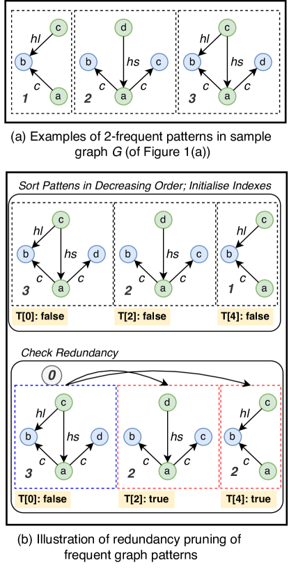
Figure 4: Frequent subgraph pruning

pairs of graph patterns for redundancy (in lines 3–9). In particular, the functions VF2U and count are used to check isomorphic matches between patterns at index $i,j$ of $\mathcal{Q}$, and compute the number of isomorphic matches returned respectively. We extended an efficient implementation of the VF2 algorithm[43] through the relaxation of some criteria as VF2U. The main difference being, in VF2U, instead of induced subgraphs, the query graph pattern simply queries subgraphs in the target graph pattern which are isomorphic to it.

For the pairwise comparison of the graph patterns, the pattern at index $j$ is considered as the query pattern whiles that at index $i$ is the target pattern. The algorithm iterates from the largest pattern in $\mathcal{Q}$ (line 3). In the round of iteration $i$, the largest pattern indexed $i$ is used as the $\mathcal{Q}(i)$ if it is tagged with $false$. As $\mathcal{Q}(j)$, every pattern indexed from $i+1$ to $n-1$ is checked to observe if it is isomorphic to $\mathcal{Q}(i)$. VF2U returns the isomorphisms from $\mathcal{Q}(j)$ to $\mathcal{Q}(i)$, and count returns the size of the resulting set.

During every iteration, the pattern indexed $j$ ($j>i$) is tagged as $true$ (i.e., line 8) if the $\mathcal{Q}(j)$ is isomorphic to the $\mathcal{Q}(i)$, and the $\mathcal{Q}(j)$ will not be a target graph in the following iterations. After all the patterns indexed from $i+1$ to $n-1$ are checked, the $\mathcal{Q}(i)$ is added into $\mathcal{Q}^{\prime}$ and the round of iteration $i$ ends. Finally, when all graph patterns have been processed, the set $\mathcal{Q}^{\prime}$ which stores all graph patterns without redundancies is returned as the output.

We present a brief illustration of the reduction process in Example 3.

Example 3 (Representative Patterns)

Given the $0.01$-dense three communities discovered in Figure 3, let the minimum support be $\tau=2$ for mining frequent subgraphs in the respective communities. Figure 4 (a) shows a list of three (3) frequent but redundant subgraphs. We illustrate the pruning strategy as follows, using the diagram in Figure 4 (b).

First, we sort the subgraphs in increasing order (of edges) and initialise the corresponding index $i$ in the vector $\vec{T}[i]$ as false. Next, we iterate over the vector, from the largest subgraph at $i$ and the next at $j=i+1$, to check the containment of the pattern at $j$ in the pattern at $i$. We set the index at $\vec{T}[j]$ to true if it contained in the patern at $i$.

Finally, we return all patterns at index $k$ if $\vec{T}[k]$ is false (in this case, pattern $3$ at index $0$). $\square$

4.1.3 Homomorphic Pattern Matching

Given the set, $\mathcal{Q}^{\prime}$, of reduced representative graph patterns from the previous step, we find their homomorphic matches in the input graph (cf. lines 9–12 of Procedure 1). To ensure efficient matching of any pattern $Q\in\mathcal{Q}^{\prime}$, we prune the input graph w.r.t. the node and edge types in $Q$ to produced a simplified/filtered version of the input graph; then perform homomorphic sub-graph matching on the simplified graph with $Q$.

A simplified graph, $G^{\prime}$, based on a given graph pattern $Q$ is a graph in which nodes and edges types (labels) that do not appear in $Q$ are removed

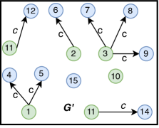
Figure 5: Simplified $G$, wrt $Q_{3}$

from the original graph, $G$. The simplification of the input graph w.r.t. a graph pattern reduces the search space of candidate matches significantly, and improves the efficiency of the matching process. We adopt the efficient worst-case optimal join (WCOJ) based algorithm introduced in [38] to find all homomorphic matches of $Q$ in $G^{\prime}$. For our running example, for brevity, suppose we want to simplify sample graph $G$, w.r.t. pattern $Q_{3}[x,y,y^{\prime}]$ in Figure 1 (a) and (d), respectively. The resulting simplified graph, $G^{\prime}$, is as shown in Figure 5.

For each set of subgraph matched records based on a graph pattern, a large attributes’ relationship data table is generated by combining all attributes of entities in the graph pattern and the values of all attributes of entities in every matched subgraph. This pseudo-relation table stores the values of all attributes of entities in a graph pattern. The first row represents all attributes of entities contained in the graph pattern, and each of the remaining rows is information about a matching subgraph, representing the values of all attributes of entities in a matched subgraph. An example of pseudo-relations over graph pattern $Q_{3}$ (from the running example in Figure 1) is presented in Figure 6.

4.2 Attribute (Entity) Dependency Discovery

Here, we mine dependencies over the pseudo-relational tables produced from the matches of the discovered graph patterns in the previous step. As depicted in Figure 2(B), the dependency discovery architecture consists of four key modules, namely: (a) Matches Preprocessor, (b) Partitioner, (c) Candidate Generator, and (d) the Validator.

In the following, we discuss the function of each module (in order), illustrating the overall dependency mining algorithm over matches $H(Q,G)$ of a pattern $Q$ in a graph $G$ (as captured in Procedure 2).

Procedure 2 mineDependencies($Q,H(Q,G)$)

1:A graph pattern $Q$, and its homomorphic matches $H(Q,G)$ in $G$

2:A set $\Sigma$ of minimal GEDs over $Q$ in $G$

3:$\Sigma:=\emptyset;\mathbb{L}[0]:=\emptyset;N:=$ no. of unique attributes in $Q$

4:$\cal{T}\leftarrow$ form pseudo-relation of $H(Q,G)$ over $Q$

5:$\mathbb{L}[1]\leftarrow generateLiteralSetPartitions(Q[\bar{u}],\cal{T})$

6:${\sf LHS}\leftarrow\mathbb{L}[0];{\sf RHS}\leftarrow\mathbb{L}[1]$

7:$\Sigma\leftarrow validateDependencies(\sf{LHS},\sf{RHS})$

8:for $i=2$ to $i=N-1$ do

9:     if $|\mathbb{L}[i-1]|>1$ then

10:         for each pair $(n_{1},n_{2})\in\mathbb{L}[i-1]\times\mathbb{L}[i-1]$ do

11:              $n=n_{1}\cup n_{2}$

12:              if $n$ is permissible then$\triangleright$ Lemma 2

13:                  $\mathbb{L}[i]:=\mathbb{L}[i]\cup n$                        

14:         ${\sf LHS}\leftarrow\mathbb{L}[i-1]$; ${\sf RHS}\leftarrow\mathbb{L}[i]$

15:         $\Sigma:=\Sigma\cup validateDependencies({\sf LHS,RHS})$      

16:return $\Sigma$

4.2.1 Pre-processing matches of patterns

This is an important (but optional) first step in the dependency mining process. In the presence of any domain-knowledge (e.g., in the form of meta data) about the input graph, one may leverage such knowledge to enhance the discovery process. For instance, given any graph pattern and its list of matches, based on available meta data, we can determine: (a) which sets of attributes to consider for each pattern variable; (b) which pairs of pattern variables to consider for the generation of variable and $id$ literals.

That is, this phase allows any relevant pre-processing of the pseudo-relational table of the matches of a graph pattern for efficient downstream mining tasks.

4.2.2 Partitioning

Next, we transform the input table into structures for efficient mining of rules. In the following, we extend the notions of equivalence classes and partitions [25] of attribute value pairs over pattern matches. This enables the adaption and use of relevant data structures, and efficient validation of candidate dependencies.

Definition 2 (Equivalence classes, partitions)

Let $H$ be the set of all matches of a graph pattern $Q[\bar{u}]$ in $G$, and $X$ be a set of literals in $\bar{u}$. The partition of $H$ by the set $X$ of literals, denoted by $\pi(X,H)$, is the set of non-empty disjoint subsets, where each subset contains all matches that satisfy $X$ with same value. For brevity, we write $\pi(X,H)$ as $\pi(X)$, when the context is clear.

Given $X,H$: $\pi(X,H)=\bigcap_{w\in X}\pi(w,H)$, where $w$  is a literal over pattern variable(s) in $Q[\bar{u}]$. Two sets of literals $X,X^{\prime}$ are equivalent w.r.t. $H$, iff: $\pi(X,H)=\pi(X^{\prime},H)$. $\square$

From the semantics of GED satisfaction and Definition 2, the following Lemma holds.

Lemma 1

A dependency $X\to Y$ holds over the pattern $Q[\bar{u}]$ in $G$ iff: $\pi(X,H)=\pi(X\cup Y,H)$.

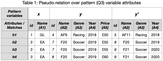
Figure 6: Example of pseudo-relation over pattern $Q_{3}$ in Figure 1(d)

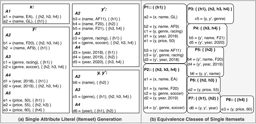
Figure 7: Example of Pattern Variable Partitions & Equivalence Classes.

Function 2 $generateLiteralSetPartitions(Q[\bar{u}],\cal{T})$

1:$\mathbb{L}[1]$ = $\emptyset$

2:for each pattern variable $x\in Q[\bar{u}]$ do$\triangleright$ constant literals

3:     for each attribute $x.A\in\cal{T}$ do

4:         $L:=\{X=(c,x.A)\mid\forall\mbox{ }c\in adom(x.A)\wedge\pi(X,H(Q,G))\neq\emptyset\}$

5:         $\mathbb{L}[1]$.add($n$): $n=(X,\pi(X,H))$      

6:for each pair $x,y\in Q[\bar{u}]$ do$\triangleright$ variable literals

7:     $L:=\{X=(x.A=y.A^{\prime})\mid A,A^{\prime}\in{\cal T}\wedge\pi(X,H(Q,G))\neq\emptyset\}$

8:     $\mathbb{L}[1]$.add($n$): $n=(X,\pi(X,H))$

9:return $\mathbb{L}[1]$

In Function 2, we presents the process of partitioning pattern variables in $Q[\bar{u}]$ of a given pseudo-relational table $\cal{T}$. Lines 2–5 generates constant literals, whereas Lines 6–8 of the function generates variable and $id$ literals. We remark that appropriate preprocessing (based on domain knowledge) from the previous step ensures only semantically meaningful pattern variable pairs are considered for variable literals.

In the following example, we show the partitions and equivalence classes of a toy example.

Example 4

Suppose pseudo-relational in Figure 6 captures the attributes of the homomorphic matches of pattern $Q_{3}$ in Figure 1. Figure 7 shows the resulting partitions and equivalence classes. We remark that, in this example, no $id$ literals are produced due to unique node identities in Figure 6.

4.2.3 Candidate dependency generation

Here, we discuss the data structures and strategies for generating candidate dependencies. We extend and model the search space of the possible dependencies with the attribute lattice [39]. We adopt a level-wise top-down search approach for generating candidate rules, testing/validating them and using the valid rules to prune the search space.

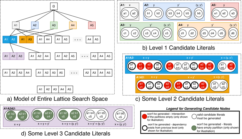
Figure 8: GED Lattice: Generation, Search & Traversal (best viewed in colour)

In general, a node $n$ in the lattice is a pair $n=(X,\pi(X))$. However, for non-redundant generation and pruning of candidate sets $X,Y$, we organise literal sets of each node under their respective pattern variable(s). For example, Figure 8 (a) shows a snapshot of the lattice for generating candidate dependencies (for the running example in Figure 6 and Figure 7). Further, parts (b), (c) and (d) of Figure 8 show all nodes in level 1, and some of the nodes for level 2 and 3 respectively.

To generate the fist level, $\mathbb{L}[1]$, nodes in the lattice, we use the single attribute partition of variables in the previous step (i.e., output of Function 2). Further, to derive nodes for higher levels of the lattice, we follow the following principles in Lemma 2 to ensure redundancy-free and valid literal set generation.

Lemma 2 (Permissible Node)

Let $\mathbb{L}[i]$ be the list of nodes at a current level $i$ of the lattice, with at least two nodes $\mathbb{L}[i]=[n_{1}=(X_{1},\pi(X_{1})),n_{2}=(X_{2},\pi(X_{2}))]$. We generate a new node $n=(X,\pi(X))\in\mathbb{L}[i+1]$ using $n_{1},n_{2}$, with the following properties: (a) $X=X_{1}\cup X_{2}$; and (b) $\pi(X)=\pi(X_{1})\cap\pi(X_{2})$. We say $n$ is permissible iff: (i) $|X|>i$, (ii) $\nexists\mbox{ }w,w^{\prime}\in X,\mbox{such that }x.A\in w,w^{\prime}$ and (iii) $\pi(X)\neq\emptyset$. $\square$

For every node pair $n_{1},n_{2}\in\mathbb{L}[i]$ that results in a permissible node $n\in\mathbb{L}[i+1]$, we establish the edges $n_{1}\to n$ and $n_{2}\to n$ representing candidate dependencies. All candidate dependencies are tested for validity in the next step. We illustrate the candidate dependency generation with our running example below.

Example 5 (Generating and searching the lattice space)

Figure 8 shows the general attribute lattice (left) and the extended literal set nodes associated with some of attribute sets (right). For brevity and clarity of presentation, we omit the partition set of nodes, and colour-code the non-permissible nodes.

Candidate rules in $\mathbb{L}[0],\mathbb{L}[1]$ are of the form: $\emptyset\to Y$, where $Y$ is a single-attribute literal in $\mathbb{L}[1]$ (i.e., every level 1 node). The set of candidate rules in $\mathbb{L}[1],\mathbb{L}[2]$ over the edge $A1\to A1A2$ take the form: $X\to Y$, where $X\in\{\{a1\},\{a2\}\}$ and $Y\in\{\{a1,b1\},\{a1,b2\},\cdots,\{a1,b6\},\{a2,b6\}\}$. $\square$

Function 3 $validateDependencies({\sf LHS,RHS})$

1:$\Sigma:=\emptyset$

2:for each node $n_{i}=(X_{i},\pi(X_{i}))\in{\sf LHS}$ do

3:     for each node $n_{j}=(Y_{j},\pi(Y_{j}))\in{\sf RHS}$ do

4:         if $X_{i}\subset Y_{j}$ and $\pi(X_{i})=\pi(Y_{j})$ then

5:              $\sigma:=(Q[\bar{u}],X_{i}\to(Y_{j}\setminus X_{i}))$

6:              $\Sigma:=\Sigma\cup\sigma$

7:              ${\sf RHS}:={\sf RHS}\setminus n_{j}$               

8:return $\Sigma$

4.2.4 Validation of dependencies

We use a level-wise traversal of search space to validate the generated candidate rules between two successive levels in the lattice. That is, for any two levels $\mathbb{L}[i]$ and $\mathbb{L}[i+1]$, correspond to the set of LHS, RHS candidates respectively. For any edge $X\to Y$ within LHS, RHS, we test the dependency $X\to Y\setminus X$. Function 3 performs this task, and its process is self-explanatory. In Line 4, $X_{i}\subset Y_{j}$ is true for all candidate dependencies (i.e., the edge $X_{i}\to Y_{j}$ exists). If the dependency holds (i.e., $\pi(X_{i})=\pi(Y_{j})$ by Lemma 1), we add the GED to the set, and prune the node search space accordingly (Lines 5–7).

In Example 6, we show the validation of some candidate GEDs in our running example.

Example 6 (Validation of candidate GEDs)

Consider the candidate GEDs in $\mathbb{L}[0],\mathbb{L}[1]$ in level 1 of the lattice, from Example 5. It is easy to verify none of the candidates are valid, since the only literal set $X\in\mathbb{L}[0]$, has the property $X=(\emptyset,\pi(\emptyset,H))$. Note that $(\pi(\emptyset,H)=\{h1,h2,h3,h4\}$. More specifically, $\pi(X)\neq\pi(X\cup Y),\forall\mbox{ }Y\in\mathbb{L}[1]$.

Similarly, we can verify the GED $X\to Y$ holds in $\mathbb{L}[1],\mathbb{L}[2]$, where $X=(\{b1\},\pi(\{b1\})),Y=(\{a1,b1\},\pi(\{a1,b1\}))$, since $\pi(\{b1\})=\pi(\{a1,b1\})$. Therefore, we can form the GED $(Q_{3}[x,y,y^{\prime}]$, $y.name=\verb|F20|\to x.name=\verb|EA|)$, and prune the node $n=(\{a1,b1\},\pi(\{a1,b1\}))\in\mathbb{L}[2]$. $\square$

4.3 Minimal cover set discovery and ranking of GEDs

In this phase of the GED mining process, we perform further analysis of all mined rules in $\Sigma$ from the previous step to determine and eliminate all redundant or implied rules. Furthermore, we introduce a measuure of interestingness to score and rank the resulting cover set $\Sigma_{c}$ of GEDs.

4.3.1 Minimal cover set

From the foregoing, every GED $\varphi\in\Sigma$ is minimal (cf., Section 3). However, $\Sigma$ may not be minimal as there may exist redundant GEDs due to the transitivity property of GEDs. More specifically, consider the following dependencies in $\Sigma:=\{\varphi_{1},\varphi_{2},\varphi_{3}\}$; where $\varphi_{1}=(Q[\bar{u}],X\to Y),\varphi_{2}=(Q[\bar{u}],Y\to Z)$ and $\varphi_{3}=(Q[\bar{u}],X\to Z)$. We say $\varphi_{3}$ is transitively implied in $\Sigma$, denoted by $\varphi_{3}\vDash\Sigma$ as $\Sigma\setminus\varphi_{3}\equiv\Sigma$. That is, the set $\Sigma^{\prime}:=\{\varphi_{1},\varphi_{2}\}\equiv\Sigma$, and $\Sigma^{\prime}$ is minimal.

Thus, it suffices to eliminate all transitively implied GEDs in $\Sigma$ to produce a minimal cover $\Sigma_{c}$ of $\Sigma$. We use a simple, but effective process in Function 4 to eliminate all transitively implied GEDs in $\Sigma$, and produce $\Sigma_{c}$. We create a graph $\Gamma$ with all GEDs in $\Sigma$ such that each node corresponds to unique literal sets of the dependencies (i.e., Lines 2, 3). We remark that, if there exists transitivity in $\Sigma$, triangles (aka. 3-cliques) will be formed in $\Gamma$ (cf., Lines 4–5), and a minimal set $\Sigma_{c}$ be returned (Lines 6–8).

Function 4 $findCover(\Sigma)$

1:$\Sigma_{c}:=\emptyset,\Gamma:=\emptyset$

2:for each $\varphi=(Q[\bar{u}],X\to Y)\in\Sigma$ do

3:     create the edge $e:X\to Y$ in $\Gamma$

4:     if $e$ completes a triangle $t\in\Gamma$ then

5:         analyse transitivity and prune $t$      

6:for each remaining edge $e\in\Gamma$ do

7:     add the corresponding GED of $e$ to $\Sigma_{c}$

8:return $\Sigma_{c}$

4.3.2 Ranking GEDs

We present a measure to score the interestingness of GEDs as well as a means to rank rules in a given minimal cover $\Sigma_{c}$. We adopt the minimum description length (MDL) principle[46] to encode the relevance of GEDs. The MDL of a model $m$ is given by:

$$mdl(m,\mbox{data})=cost(\mbox{data}|m)+\alpha\times cost(m),$$

where $cost(\mbox{data}|m)$, $cost(m)$ represent the cost of encoding errors by the model, and cost of encoding the model itself, and $\alpha$ is a hyper-parameter for trade-off between the two costs.

We propose in Equation 4.1 below a measure for scoring the interestingness, $rank(\varphi,G)$, of a GED $\varphi=(Q[\bar{u}],X\to Y)$ in a graph $G$ as:

$$rank(\varphi,G)=\alpha\times(1-\varsigma(\varphi))+(1-\alpha)\times\frac{k}{N},$$ (4.1)

where: 1) $\varsigma(\varphi)$ is the ratio $\frac{|\pi(X\cup Y)|}{|H|}\in[0,1]$, 2) $k$ is the number of unique attributes in $X\cup Y\in[0,N]$, 3) $N$ is the total number of attributes over all matches $H$ of $Q[\bar{u}]$, and 4) $\alpha\in[0,1]$ is a user-specified parameter to manipulate the trade-off between the two terms.

In line with MDL, the lower the rank of a GED, the more interesting it is. We perform an empirical evaluation of the score in the following section.

4.4 Complexity of Proposed Solution.

Here, we present sketch of the time complexity of our GED mining approach. The key tasks in our solution are: the frequent subgraph mining (FSM), and the attribute (entity) dependency mining (ADM) over the matches of the frequent subgraphs. Thus, we present the theoretical and practical complexity of both tasks below.

FSM Complexity

Let $|G|$ and $k$ denote the number of nodes in a given graph and the largest graph pattern size respectively. Overall, in the worse case, the complexity of the FSM process is ${\cal O}(2^{|G|^{2}}\cdot|G|^{k})$ (cf. details in [28]). This exponential time complexity w.r.t. $|G|$ is a major performance bottleneck, as stated in Section 1. Hence the graph splitting heuristic strategy to reduce $|G|$ via dense community detection (cf. subsection 4.1). Thus, in practice, our FSM time is ${\cal O}(C\cdot 2^{|N|^{2}}\cdot|N|^{k})\approx{\cal O}(2^{|N|^{2}}\cdot|N|^{k})$, where $C<<|N|<<|G|$ is the largest community size and $C$ is the total number of communities.

Further, performing a homomorphic matching from a $k$-sized subgraph to $G$, can be done, in the worse case, in ${\cal O}(|G|^{2}\cdot k)$ time (cf. [38] and [50]). Thus, overall time complexity for FSM is roughly ${\cal O}(2^{|N|^{2}}\cdot|N|^{k}+|G|^{2})$.

ADM Complexity

Here we examine the complexity of searching and validating all dependencies over the graph patterns. Let $|\bar{u}|$, $m$, $|H|$ be the number of nodes in a given graph pattern $Q[\bar{u}]$, maximum number of attributes per pattern variable $x\in\bar{u}$, and the total number of matches of $Q[\bar{u}]$ in $G$.

Then, the complexity of generating partitions of $H$ by literals of $\bar{u}$ is ${\cal O}(|\bar{u}|^{2}\cdot m\cdot|H|)\approx{\cal O}(m|H|)$; since in practice, $|\bar{u}|<<m<<|H|$ (cf. Function 2). Moreover, the search space of candidate GEDs is $2^{m\cdot|\bar{u}|^{2}}$. Thus, to generate, search & validate, and reduce candidate GEDs over $Q[\bar{u}]$ in $H$, requires ${\cal O}(|\bar{u}|^{2}m|H|+2^{m|\bar{u}|^{2}}|H|+|\Sigma|+|E(\Gamma)|)\approx{\cal O}(mH+2^{m}|H|+|\Sigma|)$ in the worse case (cf. Functions 3 and 4), where $|\Sigma|$ is the number of valid rules, and $|E(\Gamma)|\leq|\Sigma|$ is the total edges in the rules graph $\Gamma$.

5 Empirical Study

In this section, we present an evaluation of the proposed discovery approach using real-world graph data sets. In the following, we discuss the setting of the experiments, examine the scalability of the proposed algorithm, compared our solution to relevant related works in the literature, and demonstrate the usefulness of some of the mined GEDs in various downstream applications.

Table 2: Summary of the data sets

Data Set	#Nodes	#Edges	#Node Types	#Edge Types	Density
DBLP	300K	800K	3	3	$8.65\times 10^{-6}$
IMDB	300K	1.3M	5	8	$1.25\times 10^{-5}$
YAGO4	4.37M	13.3M	7764	83	$8.70\times 10^{-6}$

5.1 Experimental Setting

Here, we cover the data sets used and the setting of experiments.

Data Sets. We used three real-world benchmark data sets with different features and sizes, summarised in Table 2. The DBLP [40] is a citation network with 0.3M nodes of 3 types and 0.8M edges of 3 types; IMDB [41] is a knowledge graph with 0.3M nodes of 5 types and 1.3M edges of 8 types; and YAGO4 [42] is a knowledge graph with 4.37M nodes with 7764 types and 13.3M edges with 83 types. In line with [27], we use the top five most frequent attribute values in the active domain of each attribute to construct constant literals.

Experiments. All the proposed algorithms in this work were implemented in Java; and the experiments were conducted on a 2.20GHz Intel Xeon processor computer with 128GB of memory running Linux OS. We experimentally evaluated our proposed method to show its: (1) the scalability, (2) relative performance w.r.t. mining other (related) graph constraints/dependencies in the literature, (3) the potential usefulness of the mined GEDs. Unless otherwise specified, we fix the resolution parameter $\gamma$ to $1.0$, and the minimum MNI threshold $\tau$ to $5000$ in all experiments. All experiments were conducted twenty-five ($25$) times, and report the average of all results.

5.2 Scalability of proposal

Based on the complexity analysis of our proposition in Section 4.4, the key parameters that impact the time performance include: the size of the input graph $|G|$, size of graph patterns $k$, and number of attributes $m$ per pattern variable. Thus, in this set of experiments, we investigate the time performance of the proposed solution on all three data sets with respect to varying: a) input graph sizes $|G|$ (Exp-1a), b) graph pattern sizes $k$ (Exp-1b), and c) number of attributes $m$ on nodes (Exp-1c).

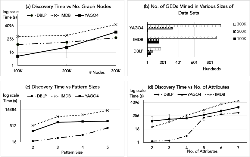
Figure 9: Scalability of proposed approach

Exp-1a. In this experiment, we fix the number of attributes on every node to seven (7) in all three data sets. We used the full graph of DBLP, sampled comparable sizes of IMDB and YAGO4 graphs. Figure 9 (a) presents a plot of the discovery time (in seconds, on a log-scale) against different sizes of the three data sets, with their corresponding standard deviations (SD) in Table 4.

Table 3: SD of Times in Figure 9 (a)

	100K	200K	300K
DBLP	$2.927$	$5.266$	$7.236$
YAGO4	$0.095$	$0.413$	$6.741$
IMDB	$4.491$	$0.749$	$23.066$

Table 4: SD of Times in Figure 9 (c)

	2	3	4	5
DBLP	$0.09$	$2.16$	$1.90$	$2.67$
YAGO4	$5.12$	$11.94$	$10.76$	$19.0$
IMDB	$7.06$	$14.30$	$23.07$	$20.95$

In general, GED discovery in the DBLP data is the most efficient as it produces the least number of matches for its frequent patterns compared to the other data sets. This characteristics is captured by the density of the graphs (in Table 2). In other words, the more dense/connected a graph is, the more likely it is to find more matches for graph patterns. Consequently, the longer the GED discovery takes.

The distribution of discovered GEDs, for different sizes of the three data sets is presented in Figure 9 (b) – with the YAGO4 and DBLP data sets producing the most and least number of GEDs in almost all cases respectively.

Exp-1b. Here, we examine the impact of graph pattern sizes on the discovery time. We use the number of nodes in a graph pattern as its size – considering patterns of size 2 to 5. For each data set, we mine GEDs over patterns size 2 to 5, using the full graph with up to seven (7) attributes per node.

The result of the time performance for different sizes of patterns are presented in Figure 9 (c), with corresponding standard deviations in Table 4. In this experiment, the IMDB and YAGO4 data sets produced comparable time performances, except for the case of patterns with size 5. In the exceptional case, we found significantly more matches of size-5 patterns in the IMDB data, which is reflected in the plot.

Exp-1c. This set of experiments examine the impact of the number of attributes on the discovery time in all data sets, varying the number of attributes on each node in the graphs from 2 to 7. The time performance of graph patterns of all sizes on the three datasets is averaged as the final result.

The plots in Figure 9 (d) show the discovery average time characteristics

Table 5: SD of Times in Figure 9 (d)

	2	3	4	5	6	7
DBLP	$0.04$	$0.02$	$0.03$	$0.07$	$0.04$	$0.27$
YAGO4	$0.02$	$0.07$	$0.06$	$0.13$	$0.27$	$0.60$
IMDB	$0.05$	$0.12$	$0.88$	$2.76$	$2.03$	$2.32$

for all three data sets with increasing number of attributes (for patterns with sizes from $2$ to $5$), with standard deviations in Table 5. As can be seen from all three line graphs, the number of attributes directly affects the time performance, as expected by the analysis of the characteristics (cf. Section 4.4).

5.3 Comparison to mining other graph constraints

The notion of GEDs generalises and sunbsumes graph functional dependencies (GFDs) and graph keys (GKeys). Thus, we show in this group of experiments that our proposal can be used for mining GFDs and GKeys via two simple adaptions. First, we replace the graph pattern matching semantics from homomorphism to isomorphism in accordance with the definitions of GFDs and GKeys. Second, we consider only id-literal RHSs for GKey mining, and no id-literals in GFD mining.

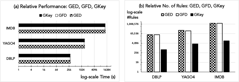
Figure 10: The performance comparison of mining GED, GFD and Gkey

In Figure 10, we present a summary of the comparative analysis of mining GEDs, GFDs and GKeys. Parts (a) of the plot represents the relative time performance of mining the three different graph constraints over the DBLP, YAGO4 and IMDB data sets respectively. In each experiment, we show the performance for up to the five (5) graph patterns (using the top five most frequent patterns in each data set).

Table 6: SD of Times in Figure 10 (a)

	GED	GFD	GKey
DBLP	$0.71$	$0.35$	$0.60$
YAGO4	$1.92$	$0.86$	$0.87$
IMDB	$15.67$	$14.85$	$16.20$

As expected, the differences in the time performances are minimal in all cases, as we have optimised: a) the matching efficiency of homomorphism vs. isomorphism; and b) the number of literals considered for each dependency/constraint type. Table 6 presents the standard deviation of the time performance on all datasets.

Furthermore, we show in Figure 10 (b) the number of discoveries for each constraint over all datasets. In particular, the number of GEDs versus GFDs is consistently similar in all datasets; and GKeys are the smallest sized rules as the RHSs are restricted to onlyid-literals.

5.4 Usefulness of mined rules

In this section, we present some examples of the discovered GEDs with a discussion of their potential use in real-world data quality and data management applications. Further, we discuss interestingness ranking of the mined GEDs.

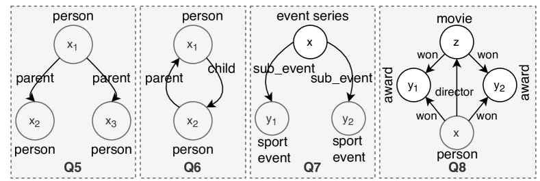
Figure 11: Graph patterns for some GEDs in YAGO4

Examples of discovered GEDs. We manually inspected the mined GEDs and validated their usefulness. We present 3 GEDs found in the YAGO4 data, with patterns shown in Figure 11 as follows:

• $Q_{5}[x_{1},x_{2},x_{3}],\{x_{1}.{\tt dob}=\verb|1777-04-24|,x_{2}.{\tt dod}=\verb|1792-03-01|,x_{3}.{\tt name}=\verb|`Leopold II, Holy Roman Emperor'|\}\to x_{2}.{\tt id}=x_{3}.{\tt id}$.

• $Q_{6}[x_{1},x_{2}],\emptyset\to x_{1}.{\tt surname}=x_{2}.{\tt surname}$.

• $Q_{7}[x,y_{1},y_{2}],x.{\tt name}=\verb|`2018 Wuhan Open'|\to x_{1}.{\tt prefixname}=x_{2}.{\tt prefixname}$.

• $Q_{8}[x,y_{1},y_{2},z],x.{\tt name}=\verb|`Akira Kurosawa'|\wedge y_{1}.{\tt name}=\verb|`Golden Lion'|\wedge y_{2}.{\tt url}=\verb|`http:www.labiennale.org'|\wedge z.{\tt name}=\verb|`Rashomon'|\to y_{1}.{\tt id}=y_{2}.{\tt id}$

The GED $\sigma_{1}$ states that for any match of the pattern $Q_{5}$ in the YAGO4 graph, if the person $x_{1}$ is born on 1777-04-24, and has a parent $x_{2}$ whose date of death is 1792-03-01 with another parent $x_{3}$ named ‘Leopard II, Holy Roman Emperor’, then $x_{2},x_{3}$ refer to the same person. This GED is verifiable true (see the Wikipedia record here) – as person $x_{1}$ is the ‘Archduchess Maria Clementina of Austria’ a child of ‘Leopard II, Holy Roman Emperor’. The discovery of $\sigma_{1}$ in the YAGO4 data signifies duplicate person entities for ‘Leopard II, Holy Roman Emperor’. Thus, a potential use for this GED can be for the disambiguation or de-duplication (entity linkage) of said entities in the graph.

Furthermore, $\sigma_{2}$ states that for any matches of the parent-child pattern $Q_{6}$, the child $x_{1}$ and parent $x_{2}$ must share the same last name. The GED $\sigma_{3}$ claims that for any two sport events $y_{1},y_{2}$ in the 2018 Wuhan Open event series $x$; $y_{1},y_{2}$ must share the same event prefixName. Indeed, these GED are straightforward and understandable; and can be used for violation or inconsistency detection in the graph through the validation of the dependencies. For example, $\sigma_{2}$ can be used to check all parent-child relationships that do not have the same surname, whiles $\sigma_{3}$ can be employed to find any sub-event in the ‘2018 Wuhan Open’ that violate the prefix-naming constraints. The GED $\sigma_{4}$, like $\sigma_{1}$, is an example of a GKey (i.e., have RHS id-literals). Thus, useful for entity resolution or de-duplication.

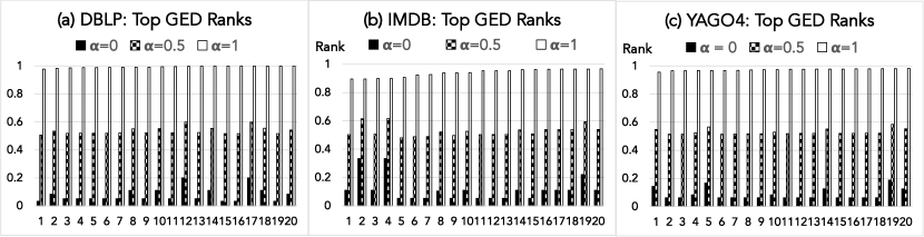
Figure 12: Top ranked GEDs w.r.t. $\alpha$ settings

The rank of GEDs. In the following, we show a plot of the interestingness scores of the discovered GEDs, for three different $\alpha$ values (i.e. 0,0.5 and 1, respectively). For brevity, and lack of space, we show the results for only the top $K=20$ GEDs in Figure 12. A lower interestingness score is representative of better GED, and vice versa. The plot shows the interestingness score is effected by the value of $\alpha$, and ranking GEDs makes it easier for users to find meaningful GEDs. For $\alpha=0$, the rank score reflects the complexity of the GED, whereas $\alpha=1$ reflects the persistence of the rule in data. And, $\alpha=0.5$ combines both with equal weight.

6 Related Work

In this section, we review related works in the literature on the discovery of graph data constraints. Mining constraints in graph data has received increasing attention in recent years. In the following, we present some relevant related works in two broad categories.

6.1 Rule discovery in non-property graphs.

Most research on profiling and mining of non-property graph data focus on XML and RDF data (cf. [47]). For instance, [48, 49, 52] investigate the problem of mining (path) association rules in RDF data and knowledge bases (KBs), whereas [53, 54, 55, 56] present inductive logic programming based rule miners over RDF data and KBs.

In contrast to the above-mentioned works, this paper studies the mining of functional (both conditional and entity) dependencies in property graphs. However, our proposed method can be adapted for mining rules in RDF data, particularly, GEDs with constant literals.

6.2 Rule discovery in property graphs.

More related to this work, are techniques for rule discovery in property graphs. Examples of some notable works in this area include: 1) [17, 27, 57, 58, 59], which investigated the discovery of association rules in property graphs; and 2) [12, 16, 22, 60] on mining keys and dependencies in property graphs—closest to this work. In particular, [12] presents a frequent sub-graph expansion based approach for mining keys in property RDFs, whiles [16] proposes efficient sequential and parallel graph functional dependency discovery for large property graphs. The main distinction between the GFD discovery approach in [16] and our work is on how the efficiency bottlenecks are handled. Specifically, [16] employs fixed parameterization to bound the sized of patterns to be mined, whereas we modulate the graph and mine graph patterns from dense communities in the graph. Furthermore, we devise a level-wise search strategy to find and validate rules via an itemset lattice, while the sequential technique in [16] finds GFDs via a vertical and horizontal spawning of generation trees.

Moreover, the work in [60] studies the discovery of temporal GFDs – GFDs that hold over property graphs over periods of time; and [22] studies the discovery of graph differential dependencies (GDDs)—GEDs with distance semantics—over property graphs. Although related, this work differs from mining temporal GFDs as we consider only one time period of graphs. And, we do not consider the semantics of difference in data as captured in GDDs. Essentially, GEDs can be considered a special case of GDDs, where the distance is zero over all attributes.

7 Conclusion

In this paper, we presented a new approach for mining GEDs. The developed discovery pipeline seamlessly combines graph partitioning, non-redundant and frequent graph pattern mining, homomorphic graph pattern matching, and attribute/entity dependencies mining to discover GEDs in property graphs. We develop effective pruning strategies and techniques to ensure the returned set of GEDs is minimal, without redundancies. Furthermore, we propose an effective MDL-based measure to score the interestingness of GEDs. Finally, we performed experiments on large real-world graphs, to demonstrate the feasibility, effectiveness and scalability of our proposal. Indeed, the empirical results are show our method is effective, salable and efficient; and finds semantically meaningful rules.

References

- [1] Fan, W., Fan, Z., Tian, C. and Dong, X.L., 2015. Keys for graphs. Proceedings of the VLDB Endowment, 8(12), pp.1590-1601.
- [2] Fan, W., Wu, Y. and Xu, J., 2016, June. Functional dependencies for graphs. In Proceedings of the 2016 International Conference on Management of Data (pp. 1843-1857).
- [3] Ma, H., Alipourlangouri, M., Wu, Y., Chiang, F. and Pi, J., 2019. Ontology-based entity matching in attributed graphs. Proceedings of the VLDB Endowment, 12(10), pp.1195-1207.
- [4] Fan, W. and Lu, P., 2017, May. Dependencies for Graphs. In 36th ACM SIGMOD-SIGACT-SIGAI Symposium on PODS (pp. 403-416). ACM.
- [5] Fan, W. and Lu, P., 2019. Dependencies for graphs. ACM Transactions on Database Systems (TODS), 44(2), pp.1-40.
- [6] Fan, W., Geng, L., Jin, R., Lu, P., Tugay, R. and Yu, W., 2022, May. Linking Entities across Relations and Graphs. In 2022 IEEE 38th International Conference on Data Engineering (ICDE) (pp. 634-647). IEEE.
- [7] Liu, J., Li, J., Liu, C. and Chen, Y., 2010. Discover dependencies from data—a review. IEEE Transactions on Knowledge and Data Engineering, 24(2), pp.251-264.
- [8] Abedjan, Ziawasch, Lukasz Golab, and Felix Naumann. ”Profiling relational data: a survey.” The VLDB Journal 24, no. 4 (2015): 557-581.
- [9] Caruccio, Loredana, Vincenzo Deufemia, and Giuseppe Polese. ”Relaxed functional dependencies—a survey of approaches.” IEEE Transactions on knowledge and data engineering 28, no. 1 (2015): 147-165.
- [10] Vezvaei, A., Golab, L., Kargar, M., Srivastava, D., Szlichta, J. and Zihayat, M., 2022. Fine-Tuning Dependencies with Parameters. In EDBT (pp. 2-393).
- [11] Zada MS, Yuan B, Anjum A, Azad MA, Khan WA, Reiff-Marganiec S. Large-scale Data Integration Using Graph Probabilistic Dependencies (GPDs). In 2020 IEEE/ACM International Conference on Big Data Computing, Applications and Technologies (BDCAT) 2020 Dec 7 (pp. 27-36). IEEE.
- [12] Alipourlangouri, M. and Chiang, F., 2018. Keyminer: Discovering keys for graphs. In VLDB workshop TD-LSG.
- [13] Kwashie, S., Liu, J., Li, J. and Ye, F., 2015, September. Conditional Differential Dependencies (CDDs). In East European Conference on Advances in Databases and Information Systems (pp. 3-17). Springer, Cham.
- [14] Kwashie, S., Liu, J., Li, J. and Ye, F., 2014, July. Mining differential dependencies: a subspace clustering approach. In Australasian Database Conference (pp. 50-61). Springer, Cham.
- [15] Kwashie, S., Liu, J., Li, J. and Ye, F., 2015, June. Efficient discovery of differential dependencies through association rules mining. In Australasian Database Conference (pp. 3-15). Springer, Cham.
- [16] Wenfei Fan, Chunming Hu, Xueli Liu, and Ping Lu. 2020. Discovering Graph Functional Dependencies. ACM Trans. Database Syst. 45, 3, Article 15 (September 2020), 42 pages.
- [17] Wenfei Fan, Xin Wang, Yinghui Wu, and Jingbo Xu. 2015. Association rules with graph patterns. Proc. VLDB Endow. 8, 12 (August 2015), 1502–1513.
- [18] Thorsten Papenbrock and Felix Naumann. 2016. A Hybrid Approach to Functional Dependency Discovery. In Proceedings of the 2016 International Conference on Management of Data (SIGMOD ’16). Association for Computing Machinery, New York, NY, USA, 821–833.
- [19] Papenbrock, Thorsten, Sebastian Kruse, Jorge-Arnulfo Quiané-Ruiz, and Felix Naumann. ”Divide & conquer-based inclusion dependency discovery.” Proceedings of the VLDB Endowment 8, no. 7 (2015): 774-785.
- [20] Lin, P., Song, Q. and Wu, Y., 2018. Fact checking in knowledge graphs with ontological subgraph patterns. Data Science and Engineering, 3(4), pp.341-358.
- [21] Fan, W., Lu, P., Tian, C. and Zhou, J., 2019. Deducing certain fixes to graphs. Proceedings of the VLDB Endowment, 12(7), pp.752-765.
- [22] Kwashie S, Liu L, Liu J, Stumptner M, Li J, Yang L. Certus: An effective entity resolution approach with graph differential dependencies (GDDs). Proceedings of the VLDB Endowment. 2019 Feb 1;12(6):653-66.
- [23] Jixue Liu, Selasi Kwashie, Jiuyong Li, Feiyue Ye, and Millist Vincent. Discovery of Approximate Differential Dependencies. cs.DB. 2013.
- [24] Chiang, Fei, and Renée J. Miller. “Discovering data quality rules.” Proceedings of the VLDB Endowment 1, no. 1 (2008): 1166-1177.
- [25] Cosmadakis, Stavros S., Paris C. Kanellakis, and Nicolas Spyratos. “Partition semantics for relations.” Journal of Computer and System Sciences 33, no. 2 (1986): 203-233.
- [26] Rammelaere, Joeri, and Floris Geerts. “Revisiting conditional functional dependency discovery: Splitting the “C” from the “FD”.” In Joint European Conference on Machine Learning and Knowledge Discovery in Databases, pp. 552-568. Springer, Cham, 2018.
- [27] Fan, W., Fu, W., Jin, R., Lu, P. and Tian, C., 2022. Discovering association rules from big graphs. Proceedings of the VLDB Endowment, 15(7), pp.1479-1492.
- [28] Mohammed Elseidy, Ehab Abdelhamid, Spiros Skiadopoulos, and Panos Kalnis. 2014. GraMi: frequent subgraph and pattern mining in a single large graph. Proc. VLDB Endow. 7, 7 (March 2014), 517–528.
- [29] Fiedler, M. and Borgelt, C., 2007, October. Subgraph support in a single large graph. In Seventh IEEE International Conference on Data Mining Workshops (ICDMW 2007) (pp. 399-404). IEEE.
- [30] Kuramochi, M. and Karypis, G., 2005. Finding frequent patterns in a large sparse graph. Data mining and knowledge discovery, 11(3), pp.243-271.
- [31] Ribeiro, P., Paredes, P., Silva, M.E., Aparicio, D. and Silva, F., 2021. A survey on subgraph counting: concepts, algorithms, and applications to network motifs and graphlets. ACM Computing Surveys (CSUR), 54(2), pp.1-36.
- [32] Jiang, C., Coenen, F., & Zito, M. (2013). A survey of frequent subgraph mining algorithms. The Knowledge Engineering Review, 28(1), 75-105. doi:10.1017/S0269888912000331
- [33] Kasra Jamshidi, Rakesh Mahadasa, & Keval Vora. 2020. Peregrine: a pattern-aware graph mining system. In Proceedings of the Fifteenth European Conference on Computer Systems (EuroSys ’20). Association for Computing Machinery, New York, NY, USA, Article 13, 1–16.
- [34] Vinicius Dias, Carlos H. C. Teixeira, Dorgival Guedes, Wagner Meira, and Srinivasan Parthasarathy. 2019. Fractal: A General-Purpose Graph Pattern Mining System. In Proceedings of the 2019 International Conference on Management of Data (SIGMOD ’19). Association for Computing Machinery, New York, NY, USA, 1357–1374.
- [35] Traag, V. A., Van Dooren, P. & Nesterov, Y. Narrow scope for resolution-limit-free community detection. Phys. Rev. E 84, 016114, https://doi.org/10.1103/PhysRevE.84.016114 (2011).
- [36] Xifeng Yan and Jiawei Han, “gSpan: graph-based substructure pattern mining,” 2002 IEEE International Conference on Data Mining, 2002. Proceedings., 2002, 721-724.
- [37] Traag, V.A., Waltman, L. & van Eck, N.J. From Louvain to Leiden: guaranteeing well-connected communities. Sci Rep 9, 5233 (2019). https://doi.org/10.1038/s41598-019-41695-z
- [38] Mhedhbi, A. and Salihoglu, S., 2019. Optimizing subgraph queries by combining binary and worst-case optimal joins. Proceedings of the VLDB Endowment, 12(11), pp.1692-1704.
- [39] R. Agrawal and R. Srikant. Fast algorithms for mining association rules in large databases. In Proceedings of the 20th International Conference on Very Large Data Bases, VLDB ’94, pages 487–499, San Francisco, CA, USA, 1994. Morgan Kaufmann Publishers Inc.
- [40] DBLP dataset. https://dblp.uni-trier.de/xml/
- [41] IMDB dataset. http://www.imdb.com/interfaces.
- [42] YAGO4 dataset. https://www.mpi-inf.mpg.de/departments/databases-and-information-systems/research/yago-naga/yago/
- [43] Luigi P. Cordella, Pasquale Foggia, Carlo Sansone, and Mario Vento, A (Sub)Graph Isomorphism Algorithm for Matching Large Graphs, IEEE Transactions on Pattern Analysis and Machine Intelligence, Vol. 26, NO. 10, 2004.
- [44] Huhtala, Yka, Juha Kärkkäinen, Pasi Porkka, and Hannu Toivonen. “TANE: An efficient algorithm for discovering functional and approximate dependencies.” The computer journal 42, no. 2 (1999): 100-111.
- [45] Bringmann B, Nijssen S. What is frequent in a single graph?. In Pacific-Asia Conference on Knowledge Discovery and Data Mining 2008 May 20 (pp. 858-863). Springer, Berlin, Heidelberg.
- [46] Peter D. Grunwald and Jorma Rissanen, The minimum description length principle, MIT Press, 2022.
- [47] Abedjan, Z., Golab, L., Naumann, F. and Papenbrock, T., 2018. Data profiling. Synthesis Lectures on Data Management, 10(4), pp.1-154.
- [48] Barati, M., Bai, Q. and Liu, Q., 2017. Mining semantic association rules from RDF data. Knowledge-Based Systems, 133, pp.183-196.
- [49] Abedjan, Z. and Naumann, F., 2013. Improving rdf data through association rule mining. Datenbank-Spektrum, 13(2), pp.111-120.
- [50] Bi, F., Chang, L., Lin, X., Qin, L. and Zhang, W., 2016, June. Efficient subgraph matching by postponing cartesian products. In Proceedings of the 2016 International Conference on Management of Data (pp. 1199-1214).
- [51] Feng, Z., Mayer, W., He, K., Kwashie, S., Stumptner, M., Grossmann, G., Peng, R. and Huang, W., 2020. A Schema-Driven Synthetic Knowledge Graph Generation Approach With Extended Graph Differential Dependencies (GDDxs). IEEE Access, 9, pp.5609-5639.
- [52] Sasaki, Y., 2022. Path association rule mining. arXiv preprint arXiv:2210.13136.
- [53] Galárraga, L.A., Teflioudi, C., Hose, K. and Suchanek, F., 2013, May. AMIE: association rule mining under incomplete evidence in ontological knowledge bases. In Proceedings of the 22nd international conference on World Wide Web (pp. 413-422).
- [54] Chen, Y., Wang, D.Z. and Goldberg, S., 2016. ScaLeKB: scalable learning and inference over large knowledge bases. The VLDB Journal, 25(6), pp.893-918.
- [55] Lajus, J., Galárraga, L. and Suchanek, F., 2020, May. Fast and exact rule mining with AMIE 3. In European Semantic Web Conference (pp. 36-52). Springer, Cham.
- [56] Ortona, S., Meduri, V.V. and Papotti, P., 2018, April. Robust discovery of positive and negative rules in knowledge bases. In 2018 IEEE 34th International Conference on Data Engineering (ICDE) (pp. 1168-1179). IEEE.
- [57] Namaki, M.H., Wu, Y., Song, Q., Lin, P. and Ge, T., 2017, November. Discovering graph temporal association rules. In Proceedings of the 2017 ACM on Conference on Information and Knowledge Management (pp. 1697-1706).
- [58] Fan, W., Jin, R., Liu, M., Lu, P., Tian, C. and Zhou, J., 2020. Capturing associations in graphs. Proceedings of the VLDB Endowment, 13(12), pp.1863-1876.
- [59] Huang, C., Zhang, Q., Guo, D., Zhao, X. and Wang, X., 2022. Discovering Association Rules with Graph Patterns in Temporal Networks. Tsinghua Science and Technology, 28(2), pp.344-359.
- [60] Noronha, L. and Chiang, F., 2021. Discovery of Temporal Graph Functional Dependencies. In Proceedings of the 30th ACM International Conference on Information & Knowledge Management (pp. 3348-3352).