Mobility Data in Operations:
The Facility Location Problem

Abstract

The recent large scale availability of mobility data, which captures individual mobility patterns, poses novel operational problems that are exciting and challenging. Motivated by this, we introduce and study a variant of the (cost-minimization) facility location problem where each individual is endowed with two locations (hereafter, her home and work locations), and the connection cost is the minimum distance between any of her locations and its closest facility. We design a polynomial-time algorithm whose approximation ratio is at most 2.497. We complement this positive result by showing that the proposed algorithm is at least a $2.428$-approximation, and there exists no polynomial-time algorithm with approximation ratio $2-\epsilon$ under UG-hardness. We further extend our results and analysis to the model where each individual is endowed with $K$ locations. Finally, we conduct numerical experiments over both synthetic data and US census data (for NYC, greater LA, greater DC, Research Triangle) and evaluate the performance of our algorithms.

1 Introduction

Individual mobility patterns have a first-order impact on many operational decisions, ranging from facility location decisions to optimization of transit systems. In the past, obtaining data on individual mobility patterns was a challenging task. However, in recent years, such data have been extensively collected through mobile phones, allowing large-scale analysis. Consequently, these valuable insights have become more accessible to decision makers, thanks to the efforts of various data providers such as Safegraph and Carto (SafeGraph, 2022; Carto, 2022).

Due to privacy concerns and data limitations, many mobility datasets (e.g., see Carto, 2023b) only record the most frequently visited places by anonymous individuals, such as their home and work locations. Decision makers can use this information to improve their decision making. One of the main applications emphasized by data providers for their mobility data is the facility location problem. An illustrative example can be found in the case of ASDA, one of the largest British supermarket chains, which leverages mobility data to make informed decisions about new facility selections (Carto, 2023a). Other practical examples include the last-mile delivery market, e.g., Lyu and Teo (2022) incorporate the mobility data and build the network of public lockers in Singapore; and the design of the bike sharing systems, for example Albuquerque et al. (2021) uses mobility data to study bike sharing stations in Lisbon.

In our paper, we aim to introduce new methodologies and important algorithmic contributions. Specifically, our research undertakes the task of formalizing the facility location problem using mobility data, providing valuable insights into how such data can enhance decision-making processes and its overall significance. We thoroughly examine the shortcomings of traditional algorithms commonly employed for facility location, propose new algorithms supported by theoretical guarantees, and present extensive numerical studies. In essence, our work delivers a comprehensive package for the study of a challenging problem that arises from the availability of new data sources. The ambition of this paper is to initiate the study of using mobility data to improve firm’s decisions.

1.1 Our contributions and techniques

We introduce and study the 2-location facility location problem (2-LFLP): A decision maker wants to choose locations of his facilities to minimize the sum of (i) facility opening costs and (ii) each individual’s “connection cost” to a facility. In the 2-LFLP, each individual is endowed with 2 locations, and her connection cost is the minimum of the distances between any of her locations and its closest facility. The majority part of this paper focuses on the 2-LFLP, and refers to each individual’s endowed locations as her home and work locations. By restricting attention to instances where the home location matches the work location for every individual, the 2-LFLP recovers the classical (single-location) metric facility location problem (MFLP). Our main result is the following:

(Main Result) For the 2-LFLP, we propose a polynomial-time algorithm (Algorithm 1) that obtains a constant approximation ratio of 2.497.

In all versions of the facility location problem (e.g., 2-LFLP, MFLP), it is natural to consider a greedy algorithm: (i) initialize all individual in the unconnected state; then (ii) iteratively pick the most cost-effective choice for unconnected individuals, i.e., either connect an unconnected individual to a facility that is already open, or open a new facility and connect a subset of unconnected individuals to this new facility. In fact, Jain et al. (2003) shows that this greedy algorithm, hereafter the JMMSV algorithm, is a 1.861-approximation for the MFLP. We show that the JMMSV algorithm no longer attains a constant-approximation guarantee in the 2-LFLP. Loosely speaking, the JMMSV algorithm fails to achieve a constant approximation ratio since the algorithm iteratively and greedily connects each unconnected individual to a facility based solely on one of her locations. However, since each individual in the 2-LFLP is endowed with two locations, the location used for the initial connection may (ex post) turn out to be quite suboptimal, thereby increasing overall costs substantially.

Motivated by the JMMSV algorithm and its failure in the 2-LFLP, we propose a new parametric family of algorithms, referred to as the 2-Chance Greedy Algorithm, which generalizes the JMMSV algorithm by allowing each individual to be connected twice (once through the home and once through the work location). This algorithm has two tuning parameters $\gamma\in[0,1]$ and $\eta\in\mathbb{R}_{+}$. The discount factor $\gamma$ discounts the cost improvement obtained by connecting individuals who were previously connected to a facility to a new one. Since each individual can be connected twice, the 2-Chance Greedy Algorithm may open more facilities than expected and lead to a high facility opening cost. To handle this, the opening cost scalar $\eta$ controls the tradeoff between the facility opening cost and the individual connection cost in the algorithm. When the discount factor $\gamma$ is set to zero and opening cost scalar $\eta$ is set to one, our algorithm recovers the JMMSV algorithm, but by choosing $\gamma>0$ appropriately, substantial cost savings can be achieved.

To characterize the performance of the 2-Chance Greedy Algorithm with discount factor $\gamma$ and opening cost scalar $\eta$, we design a family of strongly factor-revealing quadratic programs $\{\text{\hyperref@@ii[eq:strongly factor-revealing quadratic program]{$\mathcal{P}_{\texttt{SFR}}({n},\gamma,\eta)$}}\}_{{n}\in\mathbb{N}}$. We show that for any parameter $n$ the optimal objective of the corresponding program upper bounds the approximation ratio achieved by our algorithm. Using this result and setting $n=2$ we obtain a loose analytical upper bound of $\nicefrac{{6(1+\gamma)}}{{\gamma^{2}}}$ for our algorithm. Numerically solving our program we show that the optimal objective value of $\mathcal{P}_{\texttt{SFR}}(25,1,2)$ is upper bounded by 2.497, thereby yielding an approximation ratio of 2.497 for the 2-Chance Greedy Algorithm with $\gamma=1$ and $\eta=2$, as also stated above.

One implication of our approximation ratio result is as follows. In practice, the social planner can implement the 2-Chance Greedy Algorithm by varying the discount factor $\gamma$ and the opening cost scalar $\eta$, and then select the solution with the minimum cost. Our theoretical result ensures that there exists at least one parameter assignment (i.e., $\gamma=1$ and $\eta=2$) with an approximation ratio of 2.497. Nonetheless, it is possible that for the particular instance of the social planner, a better solution can be found by varying $\gamma$ and $\eta$.

It is worth highlighting that our results diverge from the prior works (e.g., Jain et al., 2003; Mahdian et al., 2006) in the literature where the approximation ratios are upperbounded by the supremum of some families of factor-revealing programs. Consequently, unlike prior works which need to analyze their factor-revealing programs for all parameters, in this work evaluating program 10 for an arbitrary ${n}\in\mathbb{N}$ provides an upperbound on the approximation ratio (and the best upper bound can be obtained by taking infimum over $n$). We refer to program 10 as the strongly factor-revealing quadratic program to emphasize this distinction.

New analysis framework: primal-dual & strongly factor-revealing quadratic program.

We rely on a primal-dual analysis to prove the bounds on the approximation ratio of the 2-Chance Greedy Algorithm. Similar to prior work, we consider a linear programming relaxation of the optimal solution and its dual program. In this dual program, there is a non-negative dual variable associated with each individual. The dual objective function is simply the sum of all these dual variables, and dual constraints impose restrictions on the sum of dual variables for every subset of individuals. The goal of the primal-dual method is to construct a dual assignment such that (i) its objective value is weakly larger than the total cost of the solution outputted by the 2-Chance Greedy Algorithm; and (ii) every dual constraint is approximately satisfied. To achieve this goal, loosely speaking, we decompose the total cost from the algorithm over individuals, and let each dual variable take the value equal to the cost of its corresponding individual. In this way, (i) is satisfied automatically. We then establish a set of structural properties of feasible execution paths generated by the 2-Chance Greedy Algorithm (Lemma 4.6), and use those to characterize the approximation factor of the dual constraints. Formally, this yields an approximation ratio for our algorithm over supremum of optimal objectives of factor-revealing programs {16}. Finally, we upperbound the optimal objective value of program 16 in terms of the infimum of strongly factor-revealing quadratic programs {10}.

Our method is (at least superficially) similar to the primal-dual analysis plus factor-revealing program for the JMMSV algorithm in the MFLP (Jain et al., 2003). However, there are two important differences in our setting that make the analysis of the 2-Chance Greedy Algorithm challenging, and differentiate our analysis from prior work : (i) Violation of triangle inequality: in the 2-LFLP, though the distance over locations in a metric space satisfies the triangle inequality, the connection cost over individuals may not satisfy the triangle inequality, (ii) Non-monotonicity of decomposed costs: the decomposed cost for each individual is not monotone increasing with respect to the time when each individual is connected (in particular, her second connection) in the 2-Chance Greedy Algorithm. Notably, while challenge (ii) is an issue for the 2-Chance Greedy Algorithm (and possibly for greedy-style algorithms in general), challenge (i) is an issue for the 2-LFLP itself (regardless of the algorithms). Both challenges have been crucial for deriving structural properties of greedy algorithms and their variants (including the JMMSV algorithm), as well as obtaining some families of factor-revealing linear program that can be analytically evaluated in prior work.

To address challenge (i), we replace a structural property induced by the triangle inequality over individuals in prior work with a weaker version induced by the triangle inequality over locations. Combining this weaker structural property and other structural properties of the 2-Chance Greedy Algorithm, we upperbound the approximation ratio of the algorithm in terms of the supremum of a family of factor-revealing programs {16}. These programs are non-linear/non-quadratic/non-convex, and thus hard to solve. To side step this difficulty, we further upperbound this supremum of programs {16} through a strongly factor-revealing quadratic program 10, which can be both analytically analyzed (albeit leading to loose bounds) and numerically computed.

The concept of strongly factor-revealing program was originally introduced by Mahdian and Yan (2011) for the competitive ratio analysis for online bipartite matching with random arrivals. To the best of our knowledge, all previous works with strongly factor-revealing programs start with a family of factor-revealing linear programs, consider some ad-hoc relaxations, and then use a naive batching argument to compress multiple variables in the original linear program into a single variable in the relaxed linear program. Invoking the linearity of both programs, the feasibility of the constructed solution from the naive batching argument is guaranteed. As a warm-up exercise, in this paper we illustrate how to use such a naive batching argument to obtain a strongly factor-revealing linear program and reprove the 1.819 for the JMMSV algorithm in the MFLP (Section 4.2.1). However, as we mentioned above, the factor-revealing program 16 for the 2-Chance Greedy Algorithm in the 2-LFLP is non-linear/non-quadratic/non-convex, and thus the naive batching argument fails (Example 4.4). Yet, we introduce a new solution-dependent batching argument, which enables us to obtain the strongly factor-revealing quadratic program 10. Given the popularity of using factor-revealing programs in the algorithm design literature, we believe our novel solution-dependent batching idea might be of independent interest.

Approximation hardness.

We complement our main results with two hardness results.

Our first hardness result is the existence of a 2-LFLP instance such that the approximation ratio of the 2-Chance Greedy Algorithm with discount factor $\gamma=1$ and opening cost scalar $\eta=2$ is at least $2.428$. We obtain this hardness result with a three-step approach. First, we construct a linear program $\mathcal{P}_{\texttt{LB}}({n})$ by introducing additional constraints into the strongly factor-revealing quadratic program $\mathcal{P}_{\texttt{SFR}}({n},1,2)$. Second, we argue that the optimal solution in program $\mathcal{P}_{\texttt{LB}}({n})$ can be converted into a 2-LFLP instance where the approximation ratio of the algorithm equals to the optimal objective of program $\mathcal{P}_{\texttt{LB}}({n})$. We then numerically evaluate program $\mathcal{P}_{\texttt{LB}}(500)$ and obtain $2.428$ as an approximation lower bound.

Our second hardness result is that no polynomial-time algorithm can obtain a approximation ratio of $2-\epsilon$ under UG-hardness (Khot, 2002) in the 2-LFLP. This approximation hardness result is directly implied by the same hardness result in the vertex cover problem (Khot and Regev, 2008), since the former generalizes the latter: consider each vertex/edge in the latter as a location/individual in the former, and let distances between locations be infinite. Notably, the 2-Chance Greedy Algorithm recovers the classic dual-fitting algorithm for the vertex cover problem instances and attains an approximation ratio of 2 for the vertex cover instances.

Extension to $K$-location FLP.

Our model admits a natural extension, which we refer to as the $K$-location facility location problem ($K$-LFLP). In $K$-LFLP, each individual is endowed with $K$ locations, e.g., her top $K$ most frequently visited places in the mobility data. The individual’s connection cost is the minimum of the distances of any of her $K$ locations and its closest facility. For this extension model, we introduce the $K$-Chance Greedy Algorithm (Algorithm 3). It is a natural generalization of the 2-Chance Greedy Algorithm, where each individual can be connected at most $K$ times through each of her locations. By properly picking the parameters of the $K$-Chance Greedy Algorithm and invoking a similar analysis, we show that the approximation ratio of the algorithm is at most the infimum of the strongly quadratic factor-revealing programs {35} over ${n}\in\mathbb{N}$. We summarize these upper bounds of the approximation ratio for $K$ between 1 and 20 in Table 5. For example, for $K=3,4,5$, the upper bounds of the approximation ratio are 3.538, 4.58, 5.611, respectively. For $K\geq 21$, the upper bound of the approximation ratio is $1.059K$. On the other hand, using the reduction from the vertex cover problem for $K$-uniform hypergraph (Khot and Regev, 2008), we show that there exists no polynomial-time algorithm with approximation ratio better than $K-\epsilon$ under UG-hardness. Therefore, the linear dependence of $K$ in our approximation ratio guarantee of the $K$-Chance Greedy Algorithm is necessary and order optimal.

Numerical simulations.

We provide a numerical justification for the performance of the 2-Chance Greedy Algorithm. We construct numerical experiments over both randomly-generated synthetic data and the US census data. For the latter, we construct 2-LFLP instances for four cities in the US: New York City (NYC), Los Angeles metropolitan area (greater LA), Washington metropolitan area (greater DC), and Raleigh-Durham-Cary CSA (Research Triangle).

We discretize the set of discount factors and opening cost scalars and compute the performance of the 2-Chance Greedy Algorithm with discount factor $\gamma\in\{0,0.2,0.4,0.6,0.8,1\}$ and opening cost scalar $\eta\in\{1,1+0.5\gamma,1+\gamma\}$. We observe that different parameters $(\gamma,\eta)$ attain the best cost for different instances, which highlights the necessity of implementing the 2-Chance Greedy Algorithm with different parameter assignments. We also obtain some structural observations: the number of opened facilities is increasing w.r.t. $\gamma$ and decreasing w.r.t. $\eta$. This aligns with the construction of the algorithm, that is, the algorithm with larger $\gamma$ (smaller $\eta$) opens facilities more aggressively since $\gamma$ amplifies ($\eta$ discounts) the value of opening additional facilities. Motivated by this, we design a post-processing step, which myopically “prunes” the solution by checking if the objective can be improved by removing any facility from the solution, and combine it with the 2-Chance Greedy Algorithm. Theoretically, adding this post-processing step does not worsen the approximation guarantee. Numerically, we observe that combing with myopic pruning, the 2-Chance Greedy Algorithm with myopic pruning further improves the performance.

Finally, we analyze the value of mobility data. Specifically, we consider a scenario where the mobility data (recording the pair of home and work locations for each individual) are missing, and a decision maker only has the residential population (resp. employment) information in each location, and then implements the JMMSV algorithm pretending that each individual can only be connected through her home (resp. work) location. In most experiments, we observe that the 2-Chance Greedy Algorithm that utilizes mobility data achieves substantially better performance than the performance of the JMMSV algorithm without mobility data.

Organization.

We start by formalizing the model and providing necessary preliminaries and notations in Section 2. In Section 3, we introduce the 2-Chance Greedy Algorithm and discuss its connection to the classic JMMSV algorithm. In Section 4, we present the approximation results of the 2-Chance Greedy Algorithm. We conduct numerical experiments over both synthetic data and US census data in Section 5. Finally, in Appendix C we extend our model, algorithm and approximation guarantee to the $K$-location FLP.

1.2 Further related work

There has been a long line of research on the (single-location) facility location problem. The 2-LFLP (and $K$-LFLP) generalizes the single-location metric facility location problem (MFLP), and can be thought as a special case of single-location non-metric facility location problem (NMFLP). Hochbaum (1982) presents a greedy algorithm with $O(\log n)$ approximation guarantee for the NMFLP. Since the first constant-approximation algorithm given by Shmoys et al. (1997) for the MFLP, several techniques and improved results have been developed around this problem (e.g., Korupolu et al., 2000; Arya et al., 2001; Jain et al., 2003; Chudak and Shmoys, 2003; Mahdian et al., 2006; Byrka, 2007). Currently, the best approximation guarantee of 1.488 is due to Li (2011); and Guha and Khuller (1999) show that it is hard to approximate within a factor of 1.463. There is another line of research on the $K$-level facility location problem, where each individual is endowed with a single location and needs to be connected with $K$ facilities in a hierarchical order. For the 2-level (resp. $K$-level) facility location problem, Zhang (2006) (resp. Aardal et al. (1999)) proposes a 1.77-approximation (resp. 3-approximation) algorithm. See survey by Ortiz-Astorquiza et al. (2018) for a comprehensive discussion. DeValve et al. (2022) study another variant of revenue-maximizing facility location problem with capacity constraint, which the authors refer as $K$-sided facility location problem. All these variants are fundamentally different from the $K$-location facility location problem studied in this paper. For example, it is hard to approximate within a factor of $K-\epsilon$ in the $K$-LFLP. In contrast, a 3-approximation polynomial time algorithm exists for the $K$-level facility location problem (Aardal et al., 1999). Due to both theoretical and practical importance of the facility location problem, there are many other variant models studied in the literature. For example, Procaccia and Tennenholtz (2013); Agrawal et al. (2022) considering strategic individuals, Meyerson (2001); Kaplan et al. (2023) considering online decision making, Wang et al. (2022) combining FLP with other combinatorial optimization problems.

There have been numerous works on different problems where the approximation or competitive ratio is determined by the infimum of a class of factor-revealing programs across a potentially large parameter space. For example, Jain et al. (2003); Mahdian et al. (2006) for the facility location problem, Mehta et al. (2002) for the AdWords problem, Mahdian and Yan (2011); Goel and Tripathi (2012) for the online matching problem, Alaei et al. (2019); Allouah and Besbes (2020); Allouah et al. (2022) in mechanism design, Correa et al. (2021) for the prophet secretary problem. Most of these works involve intricate and potentially imprecise analyses that explore the entire parameter space to obtain their final results. In contrast, Mahdian and Yan (2011); Goel and Tripathi (2012) employ the concept of strongly factor-revealing programs, which provide upper bounds on the infimum of the original factor-revealing programs by utilizing the supremum of the strongly factor-revealing programs. As a result, a single evaluation of a strongly factor-revealing program can yield the desired outcome for any given parameter. Previously, the use of strongly factor-revealing programs was primarily confined to linear programs due to their simplicity. To the best of our knowledge, our work represents the first instance of introducing a technique (the solution-dependent batching argument) that enables the derivation of a strongly non-linear factor-revealing program. Given the widespread adoption of the factor-revealing program approach, we believe that our technique holds independent interest.

2 Preliminaries

In this paper, we study the cost-minimization for the $2$-location (uncapacitated) facility location problem (2-LFLP) defined as follows.

There is a metric space $([n],d)$ with $n$ locations indexed by $[n]\triangleq\{1,\dots,n\}$ and a (metric) distance function $d:[n]\times[n]\rightarrow\mathbb{R}_{+}$. Let $E\triangleq[n]^{2}$. For each pair of locations $(i,j)\in E$, we use $\tau_{ij}$ to denote the number of individuals who reside in location $i$ and work in location $j$. We also use the notation $e=(e_{\texttt{H}},e_{\texttt{W}})\in E$ to denote individuals who reside in location $e_{\texttt{H}}$ and work in location $e_{\texttt{W}}$, and refer to $e$ as an edge between these two locations. Throughout the paper, we use the notation $(i,j)$ and $e$ interchangeably. With a slight abuse of notation, we define $\tau_{e}\triangleq\tau_{e_{\texttt{H}}e_{\texttt{W}}}$ as the number of individuals on edge $e$, and $d(e,i)\triangleq\min\{d(e_{\texttt{H}},i),d(e_{\texttt{W}},i)\}$ as the smallest distance between location $i\in[n]$ and individuals on edge $e$.

There is a social planner who wants to choose a subset $\texttt{SOL}\subseteq[n]$ as the locations of her facilities to minimize the total cost. Specifically, given an arbitrary solution $\texttt{SOL}\subseteq[n]$ as the location of facilities, the total cost $\text{\bf COST}\!\left[{\texttt{SOL}}\right]$ is defined as a combination of the facility opening cost and the individual connection cost:

$$\text{\bf COST}\!\left[{\texttt{SOL}}\right]\triangleq\displaystyle\sum_{i\in\texttt{SOL}}f_{i}+\sum_{e\in E}\tau_{e}\cdot\min_{i\in\texttt{SOL}}d(e,i)$$

where $f_{i}$ is the facility opening cost for location $i$.

Approximation.

Given a problem instance $I$, we say a solution $\texttt{SOL}\subseteq[n]$ is a $\Gamma$-approximation to the optimal solution OPT if

$$\text{\bf COST}\!\left[{\texttt{SOL}}\right]\leq\Gamma\cdot\text{\bf COST}\!\left[{\texttt{OPT}}\right]$$

where optimal solution $\texttt{OPT}\triangleq\mathop{\mathrm{arg\,min}}\limits_{\texttt{SOL}^{\prime}\subseteq[n]}\text{\bf COST}\!\left[{\texttt{SOL}^{\prime}}\right]$ is the solution minimizing the total cost.

We say an algorithm ALG is a $\Gamma$-approximation if for every problem instance $I$, the solution $\texttt{ALG}(I)$ computed from algorithm ALG is a $\Gamma$-approximation. In this paper, our goal is to design polynomial-time algorithms with constant approximation guarantees.

Proposition 2.1.

In the 2-LFLP, there exists no polynomial-time algorithm with a $2-\epsilon$ approximation guarantee under the unique game conjecture.

This hardness result is directly implied by the hardness result of the vertex cover problem (Khot and Regev, 2008). Note that the 2-LFLP generalizes the weighted vertex cover problem. See Appendix A for more discussion.

Single-location facility location problem.

The 2-LFLP generalizes the classical (single-location) metric facility location problem (MFLP) (Shmoys et al., 1997). In particular, the former problem becomes the latter problem when we further impose the restriction on the problem instances such that the home location of every individual is the same as her workspace, i.e., $\tau_{ij}=0$ for every $i\not=j$.

The 2-LFLP can also be considered as a special case of the classical (single-location) non-metric facility location problem (NMFLP) (Hochbaum, 1982). In particular, every problem instance in the 2-LFLP is equivalent to a problem instance in the NMFLP where we consider each edge $e$ as a new location with opening cost $\infty$.

The (single-location) MFLP and NMFLP have been studied extensively in the literature. Under the standard computation complexity hardness assumption, it is known that there exists no polynomial-time algorithm which can compute the optimal solution even for MFLP.

3 The 2-Chance Greedy Algorithm for the 2-LFLP

The main result of this paper is a 2.497-approximation algorithm for the 2-LFLP. In this section, we describe this algorithm and all of its ingredients. Its approximation ratio analysis with a novel strongly factor-revealing quadratic program is deferred to Section 4.

Our algorithm is a natural generalization of the classic greedy algorithm designed by Jain et al. (2003) for the single-location metric facility location problem. We first present an overview of our algorithm, followed by the formal description in Algorithm 1. Finally, we provide intuition behind our algorithm by comparing it with the classic greedy algorithm for the single-location metric/non-metric facility location problems.

Overview of the algorithm.

The 2-Chance Greedy Algorithm can be described as a continuous procedure, where we gradually identify the facilities to open in a greedy fashion and connect each edge $e\in E$ to the opened facilities. Each edge $e$ can be connected twice through both its home $e_{\texttt{H}}$ and work location $e_{\texttt{W}}$.

In this algorithm, we use SOL to denote the set of opened facilities. We maintain $\psi(e,\texttt{L})$ to record the opened facility to which edge $e\in E$ is connected through its home/work location $e_{\texttt{L}}$ for each $\texttt{L}\in\{\texttt{H},\texttt{W}\}$. Initially, we set $\psi(e,\texttt{L})\leftarrow\bot$, meaning edge $e$ has not been connected to any facility through home/work location $e_{\texttt{L}}$ yet. We further introduce an auxiliary variable $U=\{e\in E:\psi(e,\texttt{H})=\bot\land\psi(e,\texttt{W})=\bot\}$ to denote the subset of edges which have not been connected to any facilities through their home nor work locations. We say an edge $e$ is unconnected if $e\in U$, partially connected if $e\not\in U$ but $\psi(e,\texttt{H})=\bot$ or $\psi(e,\texttt{W})=\bot$, and fully connected if $\psi(e,\texttt{H})\not=\bot$ and $\psi(e,\texttt{W})\not=\bot$. Finally, we also maintain an candidate cost $\alpha(e)$ for each edge $e\in E$, which is initialized to zero, and continuously increases over time as long as edge $e$ is unconnected, i.e., $e\in U$. The algorithm terminates when all edges are partially or fully connected, i.e., $U=\emptyset$.

There are two possible events which might happen as we increase candidate cost $\alpha(e)$ for each unconnected edge $e\in U$.

Event (a): For an unconnected edge $e\in U$ the candidate cost $\alpha(e)$ equals to its per-individual connection cost $d(e,i)$ for some opened facility $i\in\texttt{SOL}$.

When Event (a) happens, we remove unconnected edge $e$ from $U$ and connect it with facility $i$ through its home/work location $e_{\texttt{L}}$ (i.e., update $\psi(e,\texttt{L})\leftarrow i$) if $\alpha(e)=d(e_{\texttt{L}},i)$ for each $\texttt{L}\in\{\texttt{H},\texttt{W}\}$. By definition, $\alpha(e)\leq d(e_{\texttt{H}},i)$, $\alpha(e)\leq d(e_{\texttt{W}},i)$ and at least one of them holds with equality.

Before we define the second event, we introduce the notion of cost improvement. For an unconnected edge $e\in U$ and an unopened facility $i$ we define per-individual cost improvement as $(\alpha(e)-d(e,i))^{+}$, where operator ${\left(x\right)^{+}}\triangleq\max\{x,0\}$. Similarly, for a partially connected edge $e$, we define discounted per-individual cost improvement as $(\gamma\alpha(e)-d(e,i))^{+}$ where discount factor $\gamma\in[0,1]$ is a pre-specified parameter of the algorithm. Intuitively, the per-individual cost improvement captures the reduction in the distance costs (relative to candidate cost) of an edge $e$ when a new facility $i$ opens and this edge is connected to it. The second event, hereafter Event (b) is as follows.

Event (b): For an unopened location $i\not\in\texttt{SOL}$, its facility opening cost ${f_{i}}$ scaled by ${\eta}$ equals to the total cost improvement associated with opening a facility at $i$. Namely, $\displaystyle\displaystyle\sum\nolimits_{e\in U}\tau_{e}\cdot{\left(\alpha(e)-d(e,i)\right)^{+}}+\displaystyle\sum\nolimits_{\vbox{\Let@\restore@math@cr\default@tag\halign{\hfil$\m@th\scriptstyle#$&$\m@th\scriptstyle{}#$\hfil\cr&e\not\in U,\\ &\texttt{L}\in\{\texttt{H},\texttt{W}\}:\psi(e,\texttt{L})=\bot\crcr}}}\tau_{e}\cdot{\left(\gamma\cdot\alpha(e)-d(e_{\texttt{L}},i)\right)^{+}}={\eta\cdot f_{i}}{}$

Here $\gamma$ and $\eta$ are two pre-specified parameters of the algorithm. The discount factor $\gamma$ controls the impact of partially connected individuals in opening new facility, while the opening cost scalar $\eta$ controls the tradeoff between facility opening cost and the individual connection cost in the solution.

When Event (b) happens, we open facility $i$ (i.e., update $\texttt{SOL}\leftarrow\texttt{SOL}\cup\{i\}$), and connect each unconnected edge $e\in U$ (resp. partially connected edge $e\not\in U:\psi(e,\texttt{L})=\bot$ for some $\texttt{L}\in\{\texttt{H},\texttt{W}\}$) with facility $i$ if $\alpha(e)\geq d(e,i)$ (resp. $\alpha(e)\geq d(e_{\texttt{L}},i)$). See Algorithm 1 for a formal description.

1

input : discount factor $\gamma\in[0,1]$, opening cost scalar $\eta\in\mathbb{R}_{+}$, 2-LFLP instance $I=(n,d,\{\tau_{e}\}_{e\in E},\{f_{i}\}_{i\in[n]})$

output : subset $\texttt{SOL}\subseteq[n]$ as the locations of opened facilities.

2

3initialize $\texttt{SOL}\leftarrow\emptyset$

4initialize $\alpha(e)\leftarrow 0$ for each edge $e\in E$

5initialize $U\leftarrow E$,

6initialize $\psi(e,\texttt{L})\leftarrow\bot$ for each edge $e\in E$, each $\texttt{L}\in\{\texttt{H},\texttt{W}\}$

7while $U\not=\emptyset$ do

8       increase $\alpha(e)$ by $d\alpha$ for every edge $e\in U$

      /* Event (a) */

9      

10      while there exists edge $e\in U$ and location $i\in\texttt{SOL}$ s.t. $\alpha(e)=d(e,i)$  do

11            

12            remove edge $e$ from $U$, i.e., $U\leftarrow U\backslash\{e\}$

13            for each $\texttt{L}\in\{\texttt{H},\texttt{W}\}$ do

14                   if $\alpha(e)=d(e_{\texttt{L}},i)$ then

15                        

16                        connect edge $e$ and facility $i$ through home/work location $e_{\texttt{L}}$, i.e., $\psi(e,\texttt{L})\leftarrow i$

17                  

18            

19      

      /* Event (b) */

20      

21      while there exists location $i\not\in\texttt{SOL}$ s.t. $∑e∈Uτe⋅(α​(e)−d​(e,i))++∑ ∉eU, subscript𝑒𝑈⋅subscript𝜏𝑒superscript𝛼𝑒𝑑𝑒𝑖subscript ∉eU, $

22       L∈{H,W}: ψ(e,L) = ⊥ τe⋅(γ⋅α(e)-d(eL,i))+=η⋅fi  do

23            

24            

25            add location $i$ into SOL, i.e., $\texttt{SOL}\leftarrow\texttt{SOL}\cup\{i\}$

26            for each edge $e\not\in U$ do

27                   for each $\texttt{L}\in\{\texttt{H},\texttt{W}\}$ do

28                        

29                        if $\psi(e,\texttt{L})=\bot$ and $\gamma\cdot\alpha(e)\geq d(e_{\texttt{L}},i)$ then

30                              

31                              connect edge $e$ and facility $i$ through home/work location $e_{\texttt{L}}$, i.e., $\psi(e,\texttt{L})\leftarrow i$

32                        

33                  

34            

35            for each edge $e\in U$ do

36                  

37                  if $\alpha(e)-d(e,i)\geq 0$ then

38                        

39                        remove edge $e$ from $U$, i.e., $U\leftarrow U\backslash\{e\}$

40                        for each $\texttt{L}\in\{\texttt{H},\texttt{W}\}$ do

41                               if $\alpha(e)\geq d(e_{\texttt{L}},i)$ then

42                                    

43                                    connect edge $e$ and facility $i$ through home/work location $e_{\texttt{L}}$, i.e., $\psi(e,\texttt{L})\leftarrow i$

44                              

45                        

46                  

47            

48      

return SOL

Algorithm 1 2-Chance Greedy Algorithm

Although Algorithm 1 is described as a deterministic continuous time procedure (due to the continuous update of candidate cost $\{\alpha(e)\}$), it is straightforward to see that the algorithm eventually terminates by construction. Furthermore, it can be executed in polynomial time. Note that Events (a) and (b) (i.e., the conditions in two while loops in lines 7 and 12) happen $O(n^{2})$ times. Thus, at any stage of the algorithm, with polynomial running time, we can identify the next time stamp in which Event (a) or (b) happens, and update all variables (i.e, SOL, $\{\psi(e,\texttt{L})\}$, $U$, $\{\alpha(e)\}$) accordingly.

Connection to the JMMSV algorithm.

For the classic single-location facility location problem, Jain et al. (2003) design a greedy-style algorithm. Throughout the paper, we denote this algorithm by the JMMSV algorithm. For completeness, we include a formal description of the JMMSV algorithm in Appendix B. Loosely speaking, the JMMSV algorithm and the 2-Chance Greedy Algorithm (Algorithm 1) use the same greedy procedure to identify facilities to open. However, the JMMSV algorithm connects each individual to a single facility, while Algorithm 1 connects each individual to one or two locations (through both her home or work location). For the single-location metric facility location problem (MFLP) where the distance function satisfies the triangle inequality, Jain et al. (2003) show that the JMMSV algorithm is a 1.861-approximation.

As we mentioned in Section 2, the 2-LFLP can also be thought as a special case of the single-location non-metric facility location problem (NMFLP), where we create a new location for each edge (but the distance between the original edges and new locations and facilities may no longer satisfy the triangle inequality). In this sense, the JMMSV algorithm is also well-defined for the 2-LFLP. Moreover, Algorithm 1 with discount factor $\gamma=0$ and opening cost scalar $\eta=1$ recovers the JMMSV algorithm for general 2-LFLP instances. To see this, observe that in Algorithm 1 with $\gamma=0$, all partially connected edges have no impact on whether new facilities will be opened at any time stamp, and every edge will be connected to exactly one facility in the end.

Observation 3.1.

In the 2-LFLP, the 2-Chance Greedy Algorithm with discount factor $\gamma=0$ and opening cost scalar $\eta=1$ is equivalent to the JMMSV algorithm.

It is known that for general NMFLP instances, the JMMSV algorithm is not constant-approximation (Hochbaum, 1982). Here we present an example to illustrate that Algorithm 1 with $\gamma=0$ and $\eta=1$, thus the JMMSV algorithm, is an $\Omega(n)$-approximation in the 2-LFLP.

Example 3.2.

Given an arbitrary $n_{0}\in\mathbb{N}$, consider a 2-LFLP instance as follows: There are $n\triangleq n_{0}+1$ locations, and $n_{0}$ individuals. Each individual $i\in[n_{0}]$ resides at location $i$. All of them work at location $n_{0}+1$. Namely, the numbers of individuals $\{\tau_{e}\}_{e\in E}$ are

$$\tau_{e}=\left\{\begin{array}[]{ll}1&\quad\text{if $e_{\texttt{H}}\in[n_{0}],e_{\texttt{W}}=n_{0}+1$}\\ 0&\quad\text{o.w.}\end{array}\right.$$

The facility opening costs $\{f_{i}\}_{i\in[n]}$ and distance function $d(\cdot,\cdot)$ are

$$f_{i}=\left\{\begin{array}[]{ll}\frac{1}{n_{0}-i+1}-\epsilon&\quad\text{if $i\in[n_{0}]$}\\ 1&\quad\text{if $i=n_{0}+1$}\end{array}\right.\qquad d(i,j)=\left\{\begin{array}[]{ll}\nicefrac{{1}}{{\eta}}&\quad\text{if $i\not=j$}\\ 0&\quad\text{if $i=j$}\end{array}\right.$$

where $\epsilon\in\mathbb{R}_{+}$ is a sufficiently small positive constant.

The optimal solution opens a facility at the common work location (i.e., $\texttt{OPT}=\{n_{0}+1\}$) with optimal total cost $\text{\bf COST}\!\left[{\texttt{OPT}}\right]=1$.

In contrast, consider the 2-Chance Greedy Algorithm with $\gamma=0$ and $\eta\in\mathbb{R}_{+}$. At time stamp $\frac{1}{n_{0}-1+1}-\epsilon$, for each edge $e$, the candidate cost $\alpha(e)=\frac{1}{n_{0}-1+1}-\epsilon$, and the condition of Event (b) for opening facility 1 is satisfied due to individual 1 residing at location 1. Thus, the algorithm opens facility $1$ and partially connects individual $1$ to facility $1$ through her home. Then, at time stamp $\frac{1}{n_{0}-2+1}-\epsilon$, the candidate cost $\alpha(e)=\frac{1}{n_{0}-2+1}-\epsilon$ for every edge $e$ except for the partially connected individual $1$, thus facility $2$ is opened, and individual $2$ is partially connected to facility $2$. Proceeding similarly, it can be seen that when the algorithm terminates, it opens $n_{0}$ facilities at every individual’s home (i.e., $\texttt{SOL}=\{1,\dots,n_{0}\}$) with total cost $\text{\bf COST}\!\left[{\texttt{SOL}}\right]=\Theta(\log(n))-n_{0}\cdot\epsilon$.

Putting all pieces together, as $\epsilon$ goes to zero, the approximation of the 2-Chance Greedy Algorithm with $\gamma=0$ converges to $\Theta(\log(n))$ for this example.

Example 3.2 also illustrates the necessity of positive discount factor $\gamma$ of Algorithm 1 to achieve a constant approximation in the 2-LFLP. Specifically, when the discount factor $\gamma$ is set as zero, Algorithm 1 never opens facility $n_{0}+1$ in the optimal solution, since the facility opening cost at location $n_{0}+1$ never meets the total cost improvement induced by candidate costs $\{\alpha(e)\}$. In particular, the candidate costs for all partially connected individuals make no positive contribution to the total cost improvement since the discount factor $\gamma=0$. Note that this issue persists if the discount factor $\gamma=o(\frac{\epsilon}{\log(n)})$. On the other hand, it is straightforward to verify that Algorithm 1 achieves a constant approximation for Example 3.2 when the discount factor $\gamma$ is set to a positive constant. In the next subsection, we further show its sufficiency by proving that Algorithm 1 with positive constant discount factor $\gamma$ is a constant-approximation for all 2-LFLP instances, e.g., a 2.497-approximation for $\gamma=1$ (Proposition 4.2, Proposition 4.4).

We finish this subsection by noting that the discount factor $\gamma$ in Algorithm 1 plays no role when we restrict attention to MFLP instances. As we mentioned in Section 2, the MFLP can be thought of as a special case of the 2-LFLP where every individual’s home is equivalent to her work location, i.e., $\tau_{e}=0$ if $e_{\texttt{H}}\not=e_{\texttt{W}}$. Therefore, Algorithm 1 is well-defined for MFLP instances. Moreover, observe that for MFLP instances, no edge $e$ with positive $\tau_{e}>0$ is ever partially connected in the algorithm. Instead, both its home $e_{\texttt{H}}$ and work location $e_{\texttt{W}}$ will be connected to the same facility in the same period. Therefore, for any fixed MFLP instance, Algorithm 1 identifies the same set of facilities SOL regardless of its discount factor $\gamma$. Thus, in this case for any discount factor $\gamma\in[0,1]$, Algorithm 1 with $\eta=1$ is equivalent to the JMMSV algorithm.

Observation 3.3.

In the MFLP, the 2-Chance Greedy Algorithm with an arbitrary discount factor $\gamma\in[0,1]$ and opening cost scalar $\eta=1$ is equivalent to the JMMSV algorithm.

To summarize our discussion, the 2-Chance Greedy Algorithm gets the best of both worlds: In the classic MFLP, for any discount factor $\gamma\in[0,1]$ and opening cost scalar $\eta=1$, the 2-Chance Greedy Algorithm recovers the JMMSV algorithm and thus is a 1.819-approximation. In the 2-LFLP, while the JMMSV algorithm degenerates to an $\Omega(\log(n))$-approximation, the 2-Chance Greedy Algorithm with a positive constant discount factor $\gamma$ remains a constant-approximation, e.g., 2.497-approximation for $\gamma=1$ and $\eta=2$, as the next section formalizes.

4 Obtaining an Approximation Ratio via Strongly Factor-Revealing Quadratic Programs

In this section, we analyze the approximation ratio of the 2-Chance Greedy Algorithm. To obtain our result, we first introduce the following quadratic program 10 parameterized by ${n}\in\mathbb{N}$, $\gamma\in[0,1]$, and $\eta\in[1,1+\gamma]$:

$$\begin{array}[]{llll}\max\limits_{\begin{subarray}{c}{f}\geq 0,\\ \mathbf{q},\bm{{\alpha}},{\mathbf{d}},{\mathbf{c}}\geq\mathbf{0}\end{subarray}}&\displaystyle\sum\nolimits_{a\in[{n}],b\in[a]}{q}(a,b)\cdot\left(\frac{1+\gamma}{\eta}\cdot{\alpha}(a,b)-\left(\frac{1+\gamma}{\eta}-1\right)\cdot{c}(a,b)\right)&\text{s.t.}&\\ \texttt{(SFR.i)}&{\alpha}(a,b)\leq{\alpha}(a^{\prime},b^{\prime})&a,a^{\prime}\in[{n}],b\in[a],b^{\prime}\in[a^{\prime}],b<b^{\prime}\\ \texttt{(SFR.ii)}&\gamma\cdot{\alpha}(a^{\prime},b^{\prime})\leq{c}(a,b)+{d}(a,b)+{d}(a^{\prime},b^{\prime})&a,a^{\prime}\in[{n}],b\in[a],b^{\prime}\in[a^{\prime}],a<a^{\prime}&\\ \texttt{(SFR.iii)}&\displaystyle\sum\nolimits_{\begin{subarray}{c}a^{\prime}\in[a+1:{n}]\\ b^{\prime}\in[a]\end{subarray}}{q}(a^{\prime},b^{\prime})\cdot{\left(\gamma\cdot{\alpha}(a^{\prime},b^{\prime})-{d}(a^{\prime},b^{\prime})\right)^{+}}&\\ &\quad+\displaystyle\sum\nolimits_{\begin{subarray}{c}a^{\prime}\in[a+1:{n}]\\ b^{\prime}\in[a+1:a^{\prime}]\end{subarray}}{q}(a^{\prime},b^{\prime})\cdot{\left(\gamma\cdot{\alpha}(a,a)-{d}(a^{\prime},b^{\prime})\right)^{+}}\leq\eta\cdot{f}&a\in[{n}-1]\\ \texttt{(SFR.iv)}&{d}(a,b)\leq{\alpha}(a,b)&a\in[{n}],b\in[a]\\ \texttt{(SFR.v)}&{c}(a,b)\leq{\alpha}(a,b)&a\in[{n}],b\in[a]\\ \texttt{(SFR.vi)}&{{f}}+\displaystyle\sum\nolimits_{a\in[{n}],b\in[a]}{q}(a,b)\cdot{d}(a,b)\leq 1&\\ \texttt{(SFR.vii)}&\displaystyle\sum\nolimits_{a\in[b:{n}]}{q}(a,b)=1&b\in[{n}]\end{array}$$ (10)

Given parameters ${n}\in\mathbb{N}$ and $\gamma\in[0,1]$, program 10 with non-negative variables ${f}$, $\{{q}(a,b),{\alpha}(a,b),{d}(a,b),{c}(a,b)\}_{a\in[{n}],b\in[a]}$ maximizes its quadratic objective over linear/quadratic constraints (SFR.i)–(SFR.vii). At a high level, constraint (SFR.ii) is derived from the triangle inequality over locations and the condition of Event (a) in the 2-Chance Greedy Algorithm, and (SFR.iii) is derived from the condition of Event (b) in the algorithm. Both the objective function and the constraints are explained in more detail in Section 4.1 and Section 4.2. Given any program $\mathcal{P}$, we denote its optimal objective value by $\text{\bf OBJ}\!\left[{\mathcal{P}}\right]$.

We are now ready to present the main result of this paper.

Theorem 4.1.

In the 2-LFLP, the approximation ratio of the 2-Chance Greedy Algorithm with discount factor $\gamma\in[0,1]$ and opening cost scalar $\eta\in[1,1+\gamma]$ is at most equal to $\Gamma_{\texttt{SFR}}(\gamma,\eta)$, where

$$\Gamma_{\texttt{SFR}}(\gamma,\eta)=\inf\limits_{{n}\in\mathbb{N}}\text{\bf OBJ}\!\left[{\text{\ref{eq:strongly factor-revealing quadratic program}}}\right]$$

We emphasize that approximation ratio $\Gamma_{\texttt{SFR}}(\gamma,\eta)$ in the above theorem is taking the infimum of $\text{\bf OBJ}\!\left[{\text{\ref{eq:strongly factor-revealing quadratic program}}}\right]$ over all possible ${n}\in\mathbb{N}$. Therefore, $\Gamma_{\texttt{SFR}}(\gamma,\eta)$ is upperbounded by $\text{\bf OBJ}\!\left[{\text{\ref{eq:strongly factor-revealing quadratic program}}}\right]$ for every ${n}\in\mathbb{N}$. This is different from the literature (e.g., Jain et al., 2003; Mahdian et al., 2006) where the approximation ratio is upperbounded by the supremum of a family of factor-revealing programs over its parameter space. Therefore, we refer to program 10 as the strongly factor-revealing quadratic program to highlight this distinction.

In practice, the social planner can implement the 2-Chance Greedy Algorithm by varying the discount factor $\gamma$ and the opening cost scalar $\eta$, and then select the solution with the minimum cost. See Section 5 for more discussion. Nonetheless, to obtain a theoretical approximation upperbound, we numerically evaluate program $\text{\bf OBJ}\!\left[{\text{\hyperref@@ii[eq:strongly factor-revealing quadratic program]{$\mathcal{P}_{\texttt{SFR}}(25,\gamma,\eta)$}}}\right]$ for every $\gamma\in\{0.1,0.2,\dots,1\}$ and $\eta\in\{1,1.1,\dots,1+\gamma\}$ with software Gurobi. Among all parameter choices in this grid search, we observe that the 2-Chance Greedy Algorithm with $\gamma=1$ and $\eta=2$ attains the best numerical approximation upperbound as follows.

Proposition 4.2.

In the 2-LFLP, the approximation ratio of the 2-Chance Greedy Algorithm with discount factor $\gamma=1$ and opening cost scalar $\eta=2$ is at most equal to $\Gamma_{\texttt{SFR}}(\gamma,\eta)\leq\text{\bf OBJ}\!\left[{\text{\hyperref@@ii[eq:strongly factor-revealing quadratic program]{$\mathcal{P}_{\texttt{SFR}}(25,1,2)$}}}\right]\leq\text{2.497}$.

We complement Proposition 4.2 with the following lower bound, and defer its formal proof to Section D.3.

Proposition 4.3.

There exists a 2-LFLP instance such that the approximation ratio of the 2-Chance Greedy Algorithm with discount factor $\gamma=1$ and opening cost scalar $\eta=2$ is at least $2.428$.

In the end of Section 3, we discuss the necessity of having a positive constant discount factor $\gamma$ to obtain a constant approximation ratio in the 2-LFLP. Here, we echo this insight by showing the following analytical but loose approximation upperbounds. See its formal proof in Section D.2.

Proposition 4.4.

In the 2-LFLP, the approximation ratio of the 2-Chance Greedy Algorithm with discount factor $\gamma\in[0,1]$ and opening cost scalar $\eta\in[1,1+\gamma]$ is at most equal to $\Gamma_{\texttt{SFR}}(\gamma,\eta)\leq\text{\bf OBJ}\!\left[{\text{\hyperref@@ii[eq:strongly factor-revealing quadratic program]{$\mathcal{P}_{\texttt{SFR}}(2,\gamma,\eta)$}}}\right]\leq\frac{6(1+\gamma)}{\gamma^{2}}$.

In the remainder of this section, we sketch the proof of Theorem 4.1 and defer some technical details to Appendix D. In Section 4.1, we first use a primal-dual framework to upperbound the approximation ratio of the 2-Chance Greedy Algorithm as the supremum over a different (and more complicated – see 16) family of factor-revealing programs, which are non-linear, non-quadratic, and non-convex. Then, we upperbound this family of factor-revealing programs through the strongly factor-revealing quadratic program 10 and complete the proof of Theorem 4.1 in Section 4.2.

4.1 Construction of factor-revealing program 16

In this part, we use the primal-dual analysis framework (initially developed by Jain et al., 2003 for the JMMSV algorithm in the MFLP) and provide three lemmas that shed light on the structure of the 2-Chance Greedy Algorithm. We then leverage these to obtain our main approximation result for 16, stated next:

Lemma 4.5.

In the 2-LFLP, the approximation ratio of the 2-Chance Greedy Algorithm with discount factor $\gamma\in[0,1]$ and opening cost scalar $\eta\in[1,1+\gamma]$ is at most equal to $\Gamma_{\texttt{FR}}(\gamma,\eta)$ where

$$\Gamma_{\texttt{FR}}(\gamma,\eta)=\sup\limits_{{m}\in\mathbb{N},\chi:[{m}]\rightarrow\tiny\mathbb{R}_{+}}\text{\bf OBJ}\!\left[{\text{\ref{eq:weakly factor-revealing program}}}\right]$$

Here 16 is the maximization program parameterized by ${m}\in\mathbb{N}$ and $\chi:[{m}]\rightarrow\tiny\mathbb{R}_{+}$ defined as follows:

$$\begin{array}[]{llll}\max\limits_{\begin{subarray}{c}{f}\geq 0,\\ \bm{{\alpha}},{\mathbf{d}},{\mathbf{c}}\geq\mathbf{0}\end{subarray}}&\displaystyle\sum\nolimits_{\ell\in[{m}]}\frac{1+\gamma}{\eta}\cdot{\alpha}(\ell)-\left(\frac{1+\gamma}{\eta}-1\right)\cdot{c}(\ell)&\text{s.t.}&\\ \texttt{(FR.i)}&\gamma\cdot{\alpha}(\ell^{\prime})\leq{c}(\ell)+{d}(\ell)+{d}(\ell^{\prime})&\ell,\ell^{\prime}\in[{m}],\chi(\ell)<\chi(\ell^{\prime})&\\ \texttt{(FR.ii)}&\displaystyle\sum\nolimits_{\ell^{\prime}\in[{m}]:\chi(\ell^{\prime})\geq\chi(\ell)}{\left(\gamma\cdot\min\left\{{\alpha}(\ell),{\alpha}(\ell^{\prime})\right\}-{d}(\ell^{\prime})\right)^{+}}\leq\eta\cdot{f}&\ell\in[{m}]\\ \texttt{(FR.iii)}&{c}(\ell)\leq{\alpha}(\ell)&\ell\in[{m}]\\ \texttt{(FR.iv)}&{{f}}{}+\displaystyle\sum\nolimits_{\ell\in[{m}]}{d}(\ell)\leq 1&\end{array}$$ (16)

In the above lemma, program 16 is parameterized by a natural number ${m}\in\mathbb{N}$, and function $\chi\in\tiny\mathbb{R}_{+}^{{m}}$ which maps $[{m}]$ to ${\tiny\mathbb{R}_{+}}$. It has non-negative variables ${f}$, $\{{\alpha}(\ell),{d}(\ell),{c}(\ell)\}_{\ell\in[{m}]}$. Function $\chi$ as a parameter of program 16 essentially specifies a total preorder over $[{m}]$, each of which in turn corresponds to different sets of constraints in (FR.i) and (FR.ii).

At a high level, constraint (FR.i) comes from the triangle inequality over locations and the condition of Event (a) of the algorithm, (FR.ii) comes from the condition of Event (b), (FR.iv) comes from the algorithm construction, and (FR.iv) is a normalization. It is worth highlighting that all constraints other than constraint (FR.ii) are linear, as is the objective function.

As we discussed after Theorem 4.1, though Lemma 4.5 already provides an upperbound $\Gamma_{\texttt{FR}}(\gamma,\eta)$ on the approximation ratio of the 2-Chance Greedy Algorithm, $\Gamma_{\texttt{FR}}(\gamma,\eta)$ is hard to be evaluated, since it is the supremum of non-linear/non-quadratic/non-convex programs {16} over all possible ${m}\in\mathbb{N}$ and $\chi\in\tiny\mathbb{R}_{+}^{{m}}$. In Section 4.2, we thus upperbound this family of factor-revealing programs  {16} through the strongly factor-revealing programs {10}, which can be both analytically analyzed (albeit leading to loose bounds) and numerically computed.

To prove Lemma 4.5, we start by identifying the structural properties of the feasible execution paths generated by the 2-Chance Greedy Algorithm. In this structural lemma, we introduce two auxiliary notations $\mathcal{Y}(\cdot,\cdot)$, $\{\sigma_{i}(\cdot)\}_{i}$ as follows. For each edge $e\in E$ and $\texttt{L}\in\{\texttt{H},\texttt{W}\}$, let $\mathcal{Y}(e,\texttt{L})$ denote the time stamp when edge $e$ is connected to facility $\psi(e,\texttt{L})$ through home/work location $e_{\texttt{L}}$ in the 2-Chance Greedy Algorithm. If $\psi(e,\texttt{L})=\bot$, we let $\mathcal{Y}(e,\texttt{L})$ be the time stamp of the termination of the algorithm. For each location $i\in[n]$, let $\sigma_{i}:E\rightarrow\{\texttt{H},\texttt{W}\}$ be the mapping such that $\sigma_{i}(e)=h$ if and only if $d(e_{\texttt{H}},i)<d(e_{\texttt{W}},i)$.

Lemma 4.6 (Structural properties of the 2-Chance Greedy Algorithm).

Given any 2-LFLP instance, after the termination of the 2-Chance Greedy Algorithm with discount factor $\gamma\in[0,1]$ and opening cost scalar $\eta\in\mathbb{R}_{+}$:

1. for every location $i\in[n]$, edges $e$, $e^{\prime}\in E$, and L, $\texttt{L}^{\prime}\in\{\texttt{H},\texttt{W}\}$, if $\mathcal{Y}(e,\texttt{L})<\mathcal{Y}(e^{\prime},\texttt{L}^{\prime})$, then $\psi(e,\texttt{L})\not=\bot$ and

   $$\gamma\cdot\alpha(e^{\prime})\leq d(e_{\texttt{L}},\psi(e,\texttt{L}))+d(e_{\texttt{L}},i)+d(e^{\prime}_{\texttt{L}^{\prime}},i)$$

2. for every location $i\in[n]$, and edge $e\in E$,

   $$\sum_{e^{\prime}\in E:\mathcal{Y}(e^{\prime},\sigma_{i}(e^{\prime}))\geq\mathcal{Y}(e,\sigma_{i}(e))}{\left(\gamma\cdot\min\left\{\alpha(e),\alpha(e^{\prime})\right\}-d(e^{\prime}_{\sigma_{i}(e^{\prime})},i)\right)^{+}}\leq\eta\cdot f_{i}$$

3. for every edge $e\in E$ and $\texttt{L}\in\{\texttt{H},\texttt{W}\}$, if $\psi(e,\texttt{L})\not=\bot$, then

   $$d(e_{\texttt{L}},\psi(e,\texttt{L}))\leq\alpha(e)$$

At a high-level, property (i) exploits the triangle inequality (of metric distance $d$ over locations) and condition of Event (a) in the algorithm; property (ii) exploits the condition of Event (b) in the algorithm; and property (iii) is implied directly from the updating rule of $\psi(e,\texttt{L})$. We defer the formal proof of Lemma 4.6 to Section D.4.

Remark 4.1.

Properties (i) – (ii) in Lemma 4.6 share similar formats as constraints (FR.i)–(FR.iii) of program 16. Loosely speaking, program 16, uses constraints (FR.i)–(FR.iii) to capture possible execution paths in the 2-Chance Greedy Algorithm. As we will see subsequently, its objective and constraint (FR.iv) is relevant for characterizing the approximation guarantee for a feasible execution path.

Remark 4.2.

In the MFLP, Jain et al. (2003) identify a structural lemma with similar properties (i) and (ii) for the JMMSV algorithm. The main difference, which becomes a new significant technical challenge in our setting, is the misalignment between $\alpha(e)$ and $\mathcal{Y}(e,\texttt{L})$. Specifically, in the 2-Chance Greedy Algorithm with strictly positive discount factor $\gamma\in(0,1]$ in the 2-LFLP, each edge $e$ may be connected to two facilities, and thus $\alpha(e)$ is not monotone with respect to the total preorder specified by $\mathcal{Y}(e,\texttt{L})$. Due to the non-monotonicity of $\alpha(e)$, the property (ii) in the structural lemma and constraint (FR.ii) in the factor-revealing program 16 include a non-linear term $\min\{\alpha(e),\alpha(e^{\prime})\}$. Consequently, program 16 becomes harder to analyze. We side step this difficulty through a major technical contribution of Section 4.2, which allows us to obtain a strongly factor-revealing quadratic program 10 that can be both analytically analyzed and numerically computed. By contrast, the JMMSV algorithm only connects each edge to a single facility, and thus $\alpha(e)\equiv\mathcal{Y}(e,\texttt{L})$ if $\psi(e,\texttt{L})\not=\bot$. Therefore, the monotonicity of $\alpha(e)$ with respect to $\mathcal{Y}(e,\texttt{L})$ is guaranteed, and the non-linear term $\min\{\alpha(e),\alpha(e^{\prime})\}$ in property (ii) simply becomes the linear term $\alpha(e)$. Consequently, both relatively simple analytical analysis and numerically-aided analysis are possible.

Remark 4.3.

Recall that the JMMSV algorithm is equivalent to the 2-Chance Greedy Algorithm with an arbitrary discount factor $\gamma\in[0,1]$ and an opening cost scalar $\eta=1$ (3.3) in the MFLP. Incorporating the monotonicity of $\alpha(e)$ discussed in Remark 4.2, the factor-revealing program 16 with $\gamma=1$ and $f=1$ recovers the factor-revealing program from Jain et al. (2003) and guarantees the 1.819-approximation of the JMMSV algorithm in the MFLP.

In what follows, we sketch a three-step argument for Lemma 4.5, and defer some details to Appendix D.

Step 1- lower bound of the optimal scaled cost via configuration LP.

Given a 2-LFLP instance, the optimal solution can be formulated as an integer program as follows. We define a service region $S=(i,\tilde{E})$ as a tuple that consists a facility at location $i$ and an edge subset $\tilde{E}\subseteq E$ that are served by facility $i$. Let $\mathcal{S}\triangleq[n]\times 2^{E}$ be the set of all possible service regions. With a slight abuse of notation, for every service region $S=(i,\tilde{E})\in\mathcal{S}$, we define its cost as $c(S)\triangleq{f_{i}}+{\sum_{e\in\tilde{E}}\tau_{e}\cdot d(e,i)}$ where the first term is the facility opening cost in location $i$, and the second term is the total connection cost between the edge $e$ and facility $i$ over all edge $e\in\tilde{E}$. To capture the optimal solution, consider an integer program where each service region $S=(i,\tilde{E})$ is associated with a binary variable $x(S)$ indicating whether the optimal solution opens facility $i$ and serves every edge $e\in\tilde{E}$ through facility $i$. Below we present its linear program relaxation 19 as well as its dual program.

$$\begin{array}[]{llllll}\min\limits_{\mathbf{x}\geq\mathbf{0}}&\displaystyle\sum\nolimits_{S\in\mathcal{S}}c(S)\cdot x(S)&\text{s.t.}&\quad\max\limits_{\bm{\mu}\geq\mathbf{0}}&\displaystyle\sum\nolimits_{e\in E}\mu(e)&\text{s.t.}\\ &\displaystyle\sum\nolimits_{S=(i,\tilde{E}):e\in\tilde{E}}x(S)\geq 1&e\in E&&\displaystyle\sum\nolimits_{e\in\tilde{E}}\mu(e)\leq c(S)&S=(i,\tilde{E})\in\mathcal{S}\end{array}$$ (19)

We formalize the connection between the optimal solution and program 19 in Lemma 4.7 and defer its formal proof into Section D.5.

Lemma 4.7.

Given any 2-LFLP instance, the optimal cost $\text{\bf COST}\!\left[{\texttt{OPT}}\right]$ is at least $\text{\bf OBJ}\!\left[{\text{\ref{eq:lp relaxtion}}}\right]$.

Step 2- dual assignment construction.

In this step, we construct the dual assignment (20) of program 19 based on the execution path of the 2-Chance Greedy Algorithm. Then we argue that the total cost of the algorithm is at most the objective value of the constructed dual assignment (Lemma 4.8). Combining with an argument that the constructed dual assignment is also approximately feasible presented in the step 3 (Lemma 4.9), the weak duality of the linear program completes the proof of Lemma 4.5.

Let SOL be the solution computed by the 2-Chance Greedy Algorithm. Let $\{\alpha(e)\}$ and $\{\psi(e,\texttt{L})\}_{e\in E,\texttt{L}\in\{\texttt{H},\texttt{W}\}}$ be the values of these variables at the termination of the algorithm. We partition all edges $e\in E$ into two disjoint subsets $E^{(1)}$ and $E^{(2)}$ as follows:

$$E^{(2)} \triangleq\{e\in E:\psi(e,\texttt{H})\not=\bot\land\psi(e,\texttt{W})\not=\bot\land\psi(e,\texttt{H})\not=\psi(e,\texttt{W})\}\qquad E^{(1)}\triangleq E\backslash E^{(2)}$$

Namely, subset $E^{(1)}$ contains every edge $e\in E$ that is either partially connected or fully connected to a single facility; while subset $E^{(2)}$ contains every edge $e\in E$ that is fully connected to two facilities.

To simplify the presentation, we assume $\psi(e,\texttt{H})\in\texttt{SOL}$ for every edge $e\in E^{(1)}$, and $d(e_{\texttt{H}},\psi(e,\texttt{H}))\leq d(e_{\texttt{W}},\psi(e,\texttt{W}))$ for edge $e\in E^{(2)}$. This is without loss of generality, since the role of home location and work location are ex ante symmetric in our model. Now, consider the dual assignment (which is not feasible in the dual problem in general) constructed as follows,

$$\begin{split}e\in E^{(1)}:&\qquad\mu(e)\leftarrow\tau_{e}\cdot\left(\frac{1+\gamma}{\eta}\cdot\alpha(e)-\left(\frac{1+\gamma}{\eta}-1\right)\cdot d(e_{\texttt{H}},\psi(e,\texttt{H}))\right)\\ e\in E^{(2)}:&\qquad\mu(e)\leftarrow\tau_{e}\cdot\left(\frac{1+\gamma}{\eta}\cdot\alpha(e)-\frac{1}{\eta}\left(d(e_{\texttt{H}},\psi(e,\texttt{H}))+d(e_{\texttt{W}},\psi(e,\texttt{W}))\right)+d(e_{\texttt{H}},\psi(e,\texttt{H}))\right)\end{split}$$ (20)

The construction of Algorithm 1 ensures that the total cost of solution SOL is upperbounded by the objective value of the constructed dual assignment. We formalize this in Lemma 4.8 and defer its formal proof to Section D.6.

Lemma 4.8.

Given any 2-LFLP instance, the total cost $\text{\bf COST}\!\left[{\texttt{SOL}}\right]$ of solution SOL computed by the 2-Chance Greedy Algorithm with discount factor $\gamma\in[0,1]$ and opening cost scalar $\eta\in\mathbb{R}_{+}$ is at most the objective value of program 19 with dual assignment (20), i.e., $\text{\bf COST}\!\left[{\texttt{SOL}}\right]\leq\sum_{e\in E}\mu(e)$.

Step 3- approximate feasibility of dual assignment.

It is straightforward to verify that the constructed dual assignment is non-negative, i.e., $\mu(e)\geq 0$ for every edge $e\in E$. It remains to show that for each service region $S=(i,\tilde{E})\in\mathcal{S}$, the dual constraint associated with primal variable $x(S)$ is approximately satisfied (with an approximation factor of $\text{\bf OBJ}\!\left[{\text{\ref{eq:weakly factor-revealing program}}}\right]$ for some parameters ${m},\chi$ depending on $S$. We formalize this in Lemma 4.9.

Lemma 4.9.

Given any 2-LFLP instance, any $\gamma\in[0,1]$ and $\eta\in[1,1+\gamma]$, for each service region $S=(i,\tilde{E})\in\mathcal{S}$, the dual assignment (20) in program 19 is approximately feasible up to multiplicative factor $\Gamma_{\texttt{FR}}(\gamma,\eta)$ where

$$\Gamma_{\texttt{FR}}(\gamma,\eta)=\sup\nolimits_{{m}\in\mathbb{N},\chi:[{m}]\rightarrow\tiny\mathbb{R}_{+}}\text{\bf OBJ}\!\left[{\text{\ref{eq:weakly factor-revealing program}}}\right]$$

In particular, fix an arbitrary service region $S=(i,\tilde{E})\in\mathcal{S}$, let $\kappa:\tilde{E}\rightarrow[{m}]$ be an arbitrary bijection from $\tilde{E}$ to $[{m}]$. Consider ${m}=|\tilde{E}|$, and $\chi(\kappa(e))=\mathcal{Y}(e,\sigma_{i}(e))$ for every edge $e\in\tilde{E}$.

$$\sum\nolimits_{e\in\tilde{E}}\mu(e)\leq\text{\bf OBJ}\!\left[{\text{\ref{eq:weakly factor-revealing program}}}\right]\cdot c(S)$$

The formal proof of Lemma 4.9 is deferred to Section D.7. At a high level, for every 2-LFLP instance, and every service region $S=(i,\tilde{E})$, we construct a solution of program 16 based on the 2-LFLP instance as well as the execution path of the 2-Chance Greedy Algorithm as follows,

$$\qquad{f}^{\dagger}\leftarrow N\cdot{f_{i}},$$

$$e\in\tilde{E}: \qquad{\alpha}^{\dagger}(\kappa(e))\leftarrow N\cdot{\alpha(e)},\quad{d}^{\dagger}(\kappa(e))\leftarrow N\cdot{d(e,i)},$$

$$e\in\tilde{E}\cap E^{(1)}: \qquad{c}^{\dagger}(\kappa(e))\leftarrow N\cdot{d}(e_{\texttt{H}},\psi(e,\texttt{H})),$$

$$e\in\tilde{E}\cap E^{(2)}: \qquad{c}^{\dagger}(\kappa(e))\leftarrow N\cdot d(e_{\sigma_{i}(e)},\psi(e,\sigma_{i}(e)))$$

where $N=\frac{1}{f_{i}+\sum_{e\in\tilde{E}}d(e,i)}$ is the normalization factor This constructed solution of program 16 is feasible: constraints (FR.i)–(FR.iii) is satisfied due to Lemma 4.6, and constraint (FR.iv) is satisfied due to the normalization factor $N$. Furthermore, its objective value equals to the ratio between $\sum_{i}\mu(e)$ over $c(S)$.

Proof of Lemma 4.5.

Invoking Lemmas 4.7, 4.8 and 4.9 and weak duality in linear programming finishes the proof. ∎

4.2 Construction of strongly factor-revealing quadratic program 10

In Lemma 4.5, we establish an upper bound on the approximation ratio of the 2-Chance Greedy Algorithm with the supremum of optimal objectives of factor revealing programs {16} over all its possible parameters ${m}\in\mathbb{N},\chi\in\tiny\mathbb{R}_{+}^{{m}}$. However, program 16 is nontrivial and does not lend itself to a straightforward characterization of this supremum. To overcome this obstacle, we upperbound the original factor-revealing program 16 through a new strongly factor-revealing quadratic program 10, and prove that the latter upperbounds the supremum of the former and, in turn, provides an approximation ratio for the algorithm. We formalize this in Lemma 4.10.

Lemma 4.10.

For any $\gamma\in[0,1]$, ${n}\in\mathbb{N}$, ${m}\in\mathbb{N}$, and $\chi:[{m}]\rightarrow\tiny\mathbb{R}_{+}$, the optimal objective value of program 16 is at most equal to the optimal objective value of program 10, i.e.,

$$\text{\bf OBJ}\!\left[{\text{\ref{eq:weakly factor-revealing program}}}\right]\leq\text{\bf OBJ}\!\left[{\text{\ref{eq:strongly factor-revealing quadratic program}}}\right]$$

The formal proof of Lemma 4.10 is deferred to Section D.8. In the remainder of this subsection, we highlight the key steps of upperbounding factor-revealing program 16 through the strongly factor-revealing quadratic program 10. Specifically, in Section 4.2.1, as a warm-up exercise, we present a simple batching argument which upperbounds the factor-revealing program 26 designed in Jain et al. (2003) for the MFLP through the strongly factor-revealing linear program 32. Consequently, we reprove the 1.819-approximation in the MFLP. Next, we discuss the main technical challenge for the 2-LFLP, and our additional treatment which upperbounds program 16 through a strongly factor-revealing quadratic program 10 in Section 4.2.2.

4.2.1 Warm-up: construction in the MFLP

In the MFLP, the 2-Chance Greedy Algorithm with an arbitrary discount factor $\gamma\in[0,1]$ and opening cost scalar $\eta=1$ is equivalent to the JMMSV algorithm (3.3), whose approximation ratio is captured by the following factor-revealing program.

Theorem 4.11 (adopted from Jain et al., 2003).

In the MFLP, the approximation ratio of the 2-Chance Greedy Algorithm with discount factor $\gamma\in[0,1]$ and opening cost scalar $\eta=1$ is equal to $\Gamma_{\texttt{FR-MFLP}}$ where

$$\Gamma_{\texttt{FR-MFLP}}=\sup\limits_{{m}\in\mathbb{N}}\text{\bf OBJ}\!\left[{\text{\ref{eq:weakly factor-revealing program MFLP}}}\right]$$

Here 26 is the maximization program parameterized by ${m}\in\mathbb{N}$ defined as follows:

$$\begin{array}[]{llll}\max\limits_{\begin{subarray}{c}{f}\geq 0,\bm{{\alpha}},{\mathbf{d}}\geq\mathbf{0}\end{subarray}}&\sum\nolimits_{\ell\in[{m}]}{\alpha}(\ell)&\text{s.t.}&\\ &{\alpha}(\ell)\leq{\alpha}(\ell^{\prime})&\ell,\ell^{\prime}\in[{m}]\\ &{\alpha}(\ell^{\prime})\leq{\alpha}(\ell)+{d}(\ell)+{d}(\ell^{\prime})&\ell,\ell^{\prime}\in[{m}]&\\ &\sum\nolimits_{\ell^{\prime}\in[\ell:{m}]}{\left({\alpha}(\ell)-{d}(\ell^{\prime})\right)^{+}}\leq{f}&\ell\in[{m}]\\ &{f}+\sum\nolimits_{\ell\in[{m}]}{d}(\ell)\leq 1&\end{array}$$ (26)

Compared to program 16 in the 2-LFLP, program 26 has an additional constraint of the monotonicity of ${\alpha}(\ell)$, and thus term ${\left(\min\{{\alpha}(\ell),{\alpha}(\ell^{\prime})\}-{d}(\ell^{\prime})\right)^{+}}$ in constraint (FR.ii) of program 16 becomes ${\left({\alpha}(\ell)-{d}(\ell^{\prime})\right)^{+}}$, which is relatively easier to handle. As a warm-up exercise, here we convert program 26 into a strongly factor-revealing program 32.

Lemma 4.12.

For any ${n}\in\mathbb{N}$, ${m}\in\mathbb{N}$,

$$\text{\bf OBJ}\!\left[{\text{\ref{eq:weakly factor-revealing program MFLP}}}\right]\leq\text{\bf OBJ}\!\left[{\text{\ref{eq:strongly factor-revealing program MFLP}}}\right]$$

where program 32 is defined as follows:

$$\begin{array}[]{llll}\max\limits_{\begin{subarray}{c}{f}\geq 0,\bm{{\alpha}},{\mathbf{d}}\geq\mathbf{0}\end{subarray}}&\sum\nolimits_{\ell\in[{n}]}{\alpha}(\ell)&\text{s.t.}&\\ &{\alpha}(\ell)\leq{\alpha}(\ell^{\prime})&\ell,\ell^{\prime}\in[{n}]\\ &{\alpha}(\ell^{\prime})\leq{\alpha}(\ell)+{d}(\ell)+{d}(\ell^{\prime})&\ell,\ell^{\prime}\in[2:{n}]&\\ &\sum\nolimits_{\ell^{\prime}\in[\ell+1:{n}]}{\left({\alpha}(\ell)-{d}(\ell^{\prime})\right)^{+}}\leq{f}&\ell\in[{n}]\\ &{f}+\sum\nolimits_{\ell\in[{n}]}{d}(\ell)\leq 1&\end{array}$$ (32)

Both program 26 and program 32 admit similar structures. The only difference is the index range in the second and third constraints. In fact, for any ${m}\in\mathbb{N}$, program $\mathcal{P}_{\texttt{SFR-MFLP}}({m})$ by construction is a relaxation of program 26, and thus $\text{\bf OBJ}\!\left[{\text{\hyperref@@ii[eq:weakly factor-revealing program MFLP]{$\mathcal{P}_{\texttt{FR-MFLP}}({m})$}}}\right]\leq\text{\bf OBJ}\!\left[{\text{\hyperref@@ii[eq:strongly factor-revealing program MFLP]{$\mathcal{P}_{\texttt{SFR-MFLP}}({m})$}}}\right]$. Lemma 4.12 is a stronger statement which establishes that $\text{\bf OBJ}\!\left[{\text{\hyperref@@ii[eq:weakly factor-revealing program MFLP]{$\mathcal{P}_{\texttt{FR-MFLP}}({m})$}}}\right]\leq\text{\bf OBJ}\!\left[{\text{\hyperref@@ii[eq:strongly factor-revealing program MFLP]{$\mathcal{P}_{\texttt{SFR-MFLP}}({n})$}}}\right]$ for every ${m},{n}\in\mathbb{N}$. Its proof is based on a simple batching argument.

Proof of Lemma 4.12.

Fix arbitrary ${n},{m}\in\mathbb{N}$. Without loss of generality, we assume that ${m}$ is sufficiently large so that $\lceil\frac{{m}}{{n}}\rceil\cdot({n}-1)\leq{m}$. Let $k=\lceil\frac{{m}}{{n}}\rceil$. Define sequence $L=\{\ell_{1},\ell_{2},\dots,\ell_{{n}},\ell_{{n}+1}\}$ where

$$\ell_{a}=\left\{\begin{array}[]{ll}1&\text{$\;~{}a=1$}\\ 1+{m}-k\cdot({n}+1-a)&\text{$\forall a\in[2:{n}+1]$}\end{array}\right.$$

By definition, $\ell_{2}-\ell_{1}={m}-k\cdot({n}-1)\leq k$, and $\ell_{a+1}-\ell_{a}=k$ for each $a\in[2:{n}]$. Given an arbitrary feasible solution $({f},\{{\alpha}(\ell),{d}(\ell)\})$ of program 26, we construct a feasible solution $({f}^{\dagger},\{{\alpha}^{\dagger}(\ell),{d}^{\dagger}(\ell)\})$ through a batching procedure as follows:

$$\qquad{f}^{\dagger}\leftarrow{f}$$

$$a\in[{n}]: \qquad{\alpha}^{\dagger}(a)\leftarrow\displaystyle\sum\nolimits_{\ell\in[\ell_{a}:\ell_{a+1}-1]}{\alpha}(\ell),\quad{d}^{\dagger}(a)\leftarrow\displaystyle\sum\nolimits_{\ell\in[\ell_{a}:\ell_{a+1}-1]}{d}(\ell)$$

See a graphical illustration of batching in Figure 1.

It is straightforward to verify that the objective value remains unchanged after the batching procedure, and all constraints are satisfied in program 32. In particular, the third constraint in program 32 for each $a\in[{n}]$ is implied by the third constraint in program 26 at $\ell=\ell_{a+1}-1$ and the convexity of ${\left(\cdot\right)^{+}}$. ∎

Figure 1: Graphical illustration of batching in Lemma 4.12: converting a feasible solution in program $\mathcal{P}_{\texttt{FR-MFLP}}(11)$ into a feasible solution in program $\mathcal{P}_{\texttt{SFR-MFLP}}(3)$.

Note that the strongly factor-revealing program 32 can be converted into a linear program by introducing additional auxiliary variables and inequalities. By numerically computing it using Gurobi, we obtain the following approximation ratio for the 2-Chance Greedy Algorithm in the MFLP.

Proposition 4.13.

In the MFLP, the approximation ratio of the 2-Chance Greedy Algorithm with discount factor $\gamma\in[0,1]$ and opening cost scalar $\eta=1$ is at most equal to $\Gamma_{\texttt{FR-MFLP}}\leq\text{\bf OBJ}\!\left[{\text{\hyperref@@ii[eq:strongly factor-revealing program MFLP]{$\mathcal{P}_{\texttt{SFR-MFLP}}(500)$}}}\right]\leq\text{1.819}$.

4.2.2 Construction in the 2-LFLP

In this part, we discuss the main technical ingredients for the proof of Lemma 4.10. We start by highlighting the additional difficulty in the analysis of 2-LFLP, and explaining the failure of the naive batching argument used in the proof of Lemma 4.12 in the MFLP. Then we focus on obtaining the strongly factor-revealing quadratic program 10, and provide one of our main technical contributions.

Failure of the naive batching argument.

In the proof of Lemma 4.12, we use a naive batching argument that groups an arbitrary feasible solution of the factor-revealing program 26 into a feasible solution in strongly factor-revealing program 32 with ${n}\leq{m}$. In particular, it divides the index set $[{m}]$ into ${n}$ consecutive subsets with almost uniform size, and groups (i.e., sums up) solutions in each consecutive subsets separately. The objective value remains unchanged, and constraints remain satisfied due to the linearity or convexity (for the third constraint in program 32).

As we highlighted at the end of Section 4.1, in the 2-LFLP, the candidate cost $\alpha(e)$ of the 2-Chance Greedy Algorithm is not monotone in the time stamp when each edge $e$ is connected, since edge $e$ can be connected twice, and its candidate cost $\alpha(e)$ stops increasing after its first connection. Therefore, the factor-revealing program program 16 does not admit the monotonicity property of ${\alpha}(\ell)$, and constraint (FR.ii) features the non-convex term $\min\{{\alpha}(\ell),{\alpha}(\ell^{\prime})\}$. Consequently, the naive batching argument fails. Here we provide an example to illustrate the failure of the naive batching argument for program 16.

Example 4.4.

Let $\chi(\ell)=\ell$ for each $\ell$. Consider a feasible solution $({f},\{{\alpha}(\ell),{d}(\ell),{c}(\ell)\}_{\ell\in[4]})$ of program $\mathcal{P}_{\texttt{FR}}(4,\chi,1,1)$ as follows: ${f}=3N$; ${\alpha}(\ell)=9N,9N,4N,14N$; ${d}(\ell)=9N,9N,4N,6N$; and ${c}(\ell)=9N,9N,4N,14N$ for $\ell=1,2,3,4$, respectively. Here $N$ is the normalization factor such that constraint (FR.iv) is satisfied with equality. It is straightforward to verify that all other constraints are also satisfied. In particular, constraint (FR.ii) at $\ell=2$ is

$$\displaystyle\sum\nolimits_{\ell^{\prime}\in[2:4]}{\left(\min\left\{{\alpha}(2),{\alpha}(\ell^{\prime})\right\}-{d}(\ell^{\prime})\right)^{+}}=\left(9N-9N\right)+\left(4N-4N\right)+\left(9N-6N\right)=3N={f}$$

Now, suppose we use the naive batching modification (defined in the proof of Lemma 4.12) to ${n}^{\dagger}=2$, the solution $({f}^{\dagger},\{{\alpha}^{\dagger}(\ell),{d}^{\dagger}(\ell),{c}^{\dagger}(\ell)\}_{\ell\in[2]})$ after the batching modification is ${f}^{\dagger}\leftarrow{f}$; ${\alpha}^{\dagger}(1)\leftarrow{\alpha}(1)+{\alpha}(2)=18N$; ${\alpha}^{\dagger}(2)\leftarrow{\alpha}(3)+{\alpha}(4)=18N$; ${d}^{\dagger}(1)\leftarrow{d}(1)+{d}(2)=18N$; ${d}^{\dagger}(1)\leftarrow{d}(1)+{d}(2)=18N$; ${c}^{\dagger}(1)\leftarrow{c}(1)+{c}(2)=18N$; and ${c}^{\dagger}(2)\leftarrow{c}(3)+{c}(4)=18N$. Notably, constraint (FR.ii) at $\ell=1$ is violated (even if we consider the similar relaxed on indexes as the one in program 32),

$$\displaystyle\sum\nolimits_{\ell^{\prime}\in[2:2]}{\left(\min\left\{{\alpha}^{\dagger}(1),{\alpha}^{\dagger}(\ell^{\prime})\right\}-{d}^{\dagger}(\ell^{\prime})\right)^{+}}=18N-10N=8N>{f}^{\dagger}$$

A solution-dependent batching argument.

To prove Lemma 4.10, we introduce a new batching argument that enables deriving the strongly factor-revealing program. Similar to the naive batching argument, given a feasible solution in the original factor-revealing program 16, the batching procedure partitions the index set and groups the variables of the original feasible solution to construct a feasible solution in the strongly factor-revealing program 10. Then we show that its objective value weakly increases and all constraints are satisfied, which ensures that the objective value of 10 upper bounds that of  16. Our new batching argument is solution-dependent, i.e., it partitions the index set into non-consecutive index subsets with non-uniform size based on the original feasible solution. Below we sketch the four major steps in our batching argument and provide intuition on our approach. All missing details and the formal proof of Lemma 4.10 is in Section D.8.

(a)

(b)

(c)

Figure 2: Graphical example illustration of steps 1, 2 and 3 in the solution-dependent batching argument for Lemma 4.10. Each combination of colors (white, gray, black) and patterns (solid, stripe, crosshatch) corresponds to an index subset $L(a,b)$. Subplot (a): pivot index subset $L=\{\ell_{1},\ell_{2},\ell_{3}\}$ and index partition $\{L(a,b)\}_{a\in[3],b\in[a]}$. Subplot (b): averaging variables in each index partition. Subplot (c): batching variables in each index partition, from one-dimensional index set $\{\ell\in[{m}]\}$ to two-dimensional index set $\{(a,b):a\in[3],b\in[a]\}$.

Step 1- identifying pivotal index subset $L$ with monotone ${\alpha}(\ell)$.

Fix an arbitrary $\gamma\in[0,1]$, $\eta\in[1,1+\gamma]$, and ${m}\in\mathbb{N}$. For ease of presentation, in this part we only consider $\chi(\cdot)$ such that $\chi(\ell)=\ell$ for each $\ell\in[{m}]$. The formal argument which covers general $\chi\in\tiny\mathbb{R}_{+}^{{m}}$ is defined in Section D.8. Suppose $({f},\{{\alpha}(\ell),{d}(\ell),{c}(\ell)\})$ is an arbitrary feasible solution of program 16. Consider a sequence of $k$ indexes $1=\ell_{1}<\ell_{2}<\dots<\ell_{k}\leq{m}$ for some $k\in\mathbb{N}$ such that

$$\forall a\in[k-1]:\qquad{\alpha}(\ell_{a})<{\alpha}(\ell_{a+1})$$

$$\forall a\in[k],~{}\forall\ell\in[\ell_{a}:\ell_{a+1}-1]:\qquad{\alpha}(\ell)\leq{\alpha}(\ell_{a})$$

where $\ell_{k+1}=m+1$. We define pivotal index subset $L\triangleq\{\ell_{a}\}_{a\in[k]}$. See Figure 2 for a graphical illustration. It is easy to show both the existence and uniqueness of pivotal index subset $L$.

Step 2- partitioning index set $[{m}]$ based on pivotal index subset $L$.

For each $a\in[k]$, $b\in[a]$, let

$$L(a,b)\triangleq\{\ell\in[\ell_{a}:\ell_{a+1}-1]:{\alpha}(\ell_{b-1})<{\alpha}(\ell)\leq{\alpha}(\ell_{b})\}$$

where ${\alpha}(\ell_{0})=0$. By definition of pivot index subset $L$, $\{L(a,b)\}_{b\in[a]}$ is a partition of $[\ell_{a}:\ell_{a+1}-1]$ for each $a\in[k]$, and $\{L(a,b)\}_{a\in[k],b\in[a]}$ is a partition of index set $[{m}]$. See Figure 2 for a graphical illustration.

Though $\{L(a,b)\}_{a\in[k],b\in[a]}$ is a partition with non-uniform size and each $L(a,b)$ may not contain a consecutive subset of indexes, it ensures the following desired monotonicity property on ${\alpha}(\ell)$: Fix $a,a^{\prime}\in[k],~{}b\in[a],~{}b^{\prime}\in[a^{\prime}]$ such that $b<b^{\prime}$. We have

$${\alpha}(\ell)\leq{\alpha}(\ell^{\prime})\qquad \forall\ell\in L(a,b),~{}\ell^{\prime}\in L(a^{\prime},b^{\prime})$$

Moreover, constraint (FR.i) in program 16 is satisfied across index subsets $$L(a,b) L(a^{\prime},b^{\prime}) a<a^{\prime} a,a^{\prime}\in[k],~{}b\in[a],~{}b^{\prime}\in[a^{\prime}] a<a^{\prime}$$ and such that . Namely, for every , if then

$$\gamma\cdot{\alpha}(\ell^{\prime})\leq{c}(\ell)+{d}(\ell)+{c}(\ell^{\prime})\qquad \forall\ell\in L(a,b),~{}\ell^{\prime}\in L(a^{\prime},b^{\prime}):$$

Finally, the monotonicity of ${\alpha}(\ell)$ across partitions $\{L(a,b)\}_{a\in[k],b\in[a]}$ also enables us to remove non-convex term $\min\{{\alpha}(\ell),{\alpha}(\ell^{\prime})\}$ in constraint (FR.ii) in program 16 at $\ell=\ell_{a}$. Namely, for every $a\in[k-1]$, the aforementioned constraint can be rewritten as follows:

$$\sum_{a^{\prime}\in[a:k]}\sum_{b^{\prime}\in[a]}\sum_{\ell^{\prime}\in L(a^{\prime},b^{\prime})}{\left(\gamma\cdot{\alpha}(\ell^{\prime})-{d}(\ell^{\prime})\right)^{+}}+\sum_{a^{\prime}\in[a:k]}\sum_{b^{\prime}\in[a+1:a^{\prime}]}\sum_{\ell^{\prime}\in L(a^{\prime},b^{\prime})}{\left(\gamma\cdot{\alpha}(\ell_{a})-{d}(\ell^{\prime})\right)^{+}}\leq{f}.$$

Step 3- batching variables based on partitions $\{L(a,b)\}_{a\in[k],b\in[a]}$

Partitions $\{L(a,b)\}_{a\in[k],b\in[a]}$ nicely preserve the feasibility of all constraints (for most indexes) in program 16 (as illustrated in the previous step). This suggests a natural batching procedure for constructing a solution to $\mathcal{P}_{\texttt{SFR}}(k,\gamma,\eta)$ that involves grouping variables in each $L(a,b)$ separately. Since the size of each $L(a,b)$ is not identical, we introduce additional variables $\{{q}(a,b)\}_{a\in[k],b\in[a]}$ to keep track of the size. Consequently, we construct a solution $({f}^{\dagger},\{{q}^{\dagger}(a,b),{\alpha}^{\dagger}(a,b),{d}^{\dagger}(a,b),{c}^{\dagger}(a,b)\})$ for program $\mathcal{P}_{\texttt{SFR}}(k,\gamma,\eta)$ as follows,

$${f}^{\dagger}\leftarrow{f}$$

$$a\in[k],b\in[a]:\qquad {\alpha}^{\dagger}(a,b)\leftarrow\sum_{\ell\in L(a,b)}\frac{{\alpha}(\ell)}{|L(a,b)|},\quad{d}^{\dagger}(a,b)\leftarrow\sum_{\ell\in L(a,b)}\frac{{d}(\ell)}{|L(a,b)|},$$

$${c}^{\dagger}(a,b)\leftarrow\sum_{\ell\in L(a,b)}\frac{{c}(\ell)}{|L(a,b)|},\quad{q}^{\dagger}(a,b)\leftarrow|L(a,b)|$$

See Figure 2 for a graphical illustration.

It can be verified that the objective value remains unchanged, and all constraints of program $\mathcal{P}_{\texttt{SFR}}(k,\gamma,\eta)$ (except constraints (SFR.iv) and (SFR.vii)) are satisfied. In the formal proof in Section D.8, we show that imposing constraint (SFR.iv), does not change the optimal objective value. We discuss how to handle constraint (SFR.vii), in the next step.

Step 4- converting into a feasible solution of program 10.

In the last step, we further convert the solution obtained in step 3 for program $\mathcal{P}_{\texttt{SFR}}(k,\gamma,\eta)$ into a feasible solution for program 10 for an arbitrary ${n}\in\mathbb{N}$. The formal argument is not difficult but quite detailed. All technical details can be found in Section D.8.

The main technical difficulty in this step is to design a batching procedure that guarantees the feasibility of constraint (SFR.vii), i.e., $\forall b\in[{n}]:\sum_{a\in[b:{n}]}{q}(a,b)=1$. To overcome this difficulty, we first apply a decomposition procedure (see Figure 6 in the appendix) which converts the solution in program $\mathcal{P}_{\texttt{SFR}}(k,\gamma,\eta)$ into a solution in program $\mathcal{P}_{\texttt{SFR}}(k^{\dagger},\gamma,\eta)$ with $k^{\dagger}\geq k$ such that the total mass $\sum_{a\in[b:k^{\dagger}]}{q}(a,b)$ is sufficiently small for each $b\in[k^{\dagger}]$. This enables us to identify a sequence $0=b_{0}<b_{1}<b_{2}<\dots<b_{{n}}=k^{\dagger}$ such that for every $t\in[{n}]$, $\sum_{b\in[b_{t-1}+1:b_{t}]}\sum_{a\in[b:n]}{q}(a,b)=1$. Then, we apply another batching procedure (see Figure 7 in the appendix) based on sequence $\{b_{t}\}_{t\in[{n}]}$, and obtain a feasible solution in program 10, whose objective value is weakly higher than the the objective value of the original solution in step 1, as desired. It is worthwhile highlighting that both the decomposition and the batching procedure in this step heavily rely on the the monotonicity property imposed in constraint (SFR.i), which is established in Steps 1 and 2 based on pivot index subset $L$ and its induced solution-dependent index partitions.

5 Numerical Experiments

To provide numerical justifications for the performance of our proposed algorithm, we performed numerical experiments on both synthetic data (Section 5.1) and US census data (Section 5.2).

5.1 Experiments over synthetic data

We first discuss the numerical experiment over randomly-generated synthetic data.

Experimental setup.

In our test problem, there are $n=30$ locations. Each location $i\in[n]$ is associated with a two-dimensional coordinate $(x_{i},y_{i})$, population $N_{i}$, and facility opening cost $f_{i}$. Here, coordinates $x_{i},y_{i}$ are drawn i.i.d. from the normal distribution $\texttt{Normal}(0,1)$, population $N_{i}$ is drawn i.i.d. from the exponential distribution $\texttt{Exponential}(\nicefrac{{1}}{{100}})$, and facility opening cost $f_{i}$ is drawn i.i.d. from the exponential distribution $\texttt{Exponential}(\nicefrac{{1}}{{\bar{f}}})$ with $\bar{f}\in\{20,100\}$. We consider the Euclidean distance based on coordinates $\{(x_{i},y_{i})\}$ as the distance function $d:[n]\times[n]\rightarrow\mathbb{R}_{+}$.

The number of individuals $\tau_{ij}$ for each edge $(i,j)\in E$ is generated as follows. Each location $i\in[n]$ is associated with an employee attractiveness $\rho_{i}$ drawn i.i.d. from the exponential distribution $\texttt{Exponential}(1)$. For each edge $(i,j)\in E$, we set

$$\tau_{ij}\triangleq\displaystyle N_{i}\cdot\frac{\rho_{j}\cdot\exp\left(-\iota\cdot d(i,j)\right)}{\sum_{k\in[n]}\rho_{k}\cdot\exp\left(-\iota\cdot d(i,k)\right)}$$

In this construction, $\tau_{ij}$ is inline with the standard MNL model by interpreting $\log(\rho_{j})-\iota\cdot d(i,j)$ as the value of working at location $j$ for individuals who reside in location $i$. Consequently, $\tau_{ij}$ increases as the employee attractiveness $\rho_{j}$ of location $j$ increases. Parameter $\iota$ controls the impact of distance between locations $i$ and $j$ on $\tau_{ij}$. Here we present results for $\iota=\nicefrac{{1}}{{5}}$.

Policies.

In this numerical experiment, we compare three different classes of policies:

1. The 2-Chance Greedy Algorithm: this policy is Algorithm 1 parameterized by discount factor $\gamma$ and opening cost scalar $\eta$. Its approximation ratio is upperbounded by $\Gamma_{\texttt{SFR}}(\gamma,\eta)$. We implement this policy with discount factor $\gamma\in\{0,0.2,0.4,0.6,0.8,1\}$ and opening cost scalar $\eta\in\{1,1+0.5\gamma,1+\gamma\}$, and refer it as $\texttt{2-GR}(\gamma,\eta)$. Recall that the JMMSV algorithm is a special case, i.e., $\texttt{2-GR}(0,1)$ (3.1). Hereafter, we use $\texttt{Param}\triangleq\{(\gamma,\eta):\gamma\in\{0,0.2,0.4,0.6,0.8,1\},\eta\in\{1,1+0.5\gamma,1+\gamma\}\}$ to denote the space of discretized $\gamma$ and $\eta$ in our experiments.

   Moreover, for each randomly generated instance, we compute the total cost of $\texttt{2-GR}(\gamma,\eta)$ for all discretized $(\gamma,\eta)\in\texttt{Param}$ described above, and then refer the best one as $\texttt{2-GR}^{*}$. Namely, for each randomly generated instance $I$, $\texttt{2-GR}^{*}\triangleq\texttt{2-GR}(\gamma^{*},\eta^{*})$ with

   $$(\gamma^{*},\eta^{*})=\mathop{\mathrm{arg\,min}}_{(\gamma,\eta)\in\texttt{Param}}\text{\bf COST}_{I}\!\left[{\texttt{2-GR}(\gamma,\eta)}\right]$$

   where $\text{\bf COST}_{I}\!\left[{\texttt{2-GR}(\gamma,\eta)}\right]$ is the total cost of algorithm $\texttt{2-GR}(\gamma,\eta)$ on instance $I$.

2. The 2-Chance Greedy Algorithm with Myopic Pruning: this policy combines Algorithm 1 with an additional post-processing step (i.e., myopic pruning) as follows. Given SOL returned by Algorithm 1, this policy iteratively checks whether the total cost can be reduced by removing (a.k.a., pruning) a facility from current solution SOL. If such a facility exists, it greedily prunes the one with the highest cost reduction, and repeats. By construction, the performance of this policy is weakly better than the original 2-Chance Greedy Algorithm, and its approximation ratio is upperbouned by $\Gamma_{\texttt{SFR}}(\gamma,\eta)$ as well. We implement this policy with discretized discount factor $\gamma$ and opening cost scalar $\eta$ for all $(\gamma,\eta)\in\texttt{Param}$, and refer it as $\texttt{2-GRP}(\gamma,\eta)$. Similar to $\texttt{2-GR}^{*}$, we introduce $\texttt{2-GRP}^{*}$ to denote algorithm $\texttt{2-GRP}(\gamma,\eta)$ with the best discretized $(\gamma,\eta)$ for each randomly generated instance.

3. The Greedy Algorithm with Home (resp. Work) Location: this policy is the JMMSV algorithm (Jain et al., 2003, Algorithm 2) assuming that each individual can only be connected through her home (resp. work) location. This policy requires the knowledge of population $\{N_{i}\}$ (resp. employment) for each location, and the knowledge of $\{\tau_{ij}\}$ is unnecessary. Its approximation ratio in the 2-LFLP is unbounded. We refer this policy as GR-H (resp. GR-W).

Results.

In order to compare different policies, we sample 100 randomly generated synthetic instances. For each instance and each policy, we normalize its performance by computing the ratio between the cost of this policy on this instance and the cost of policy $\texttt{2-GRP}^{*}$. Below we discuss our numerical results in detail.

Table 1: Average costs for different policies in Section 5.1.

	$\texttt{2-GR}^{*}$	$\texttt{2-GRP}^{*}$	GR-H	GR-W
$\bar{f}=20$	236.23	235.59	302.03	298.63
$\bar{f}=100$	599.27	597.94	682.28	680.71

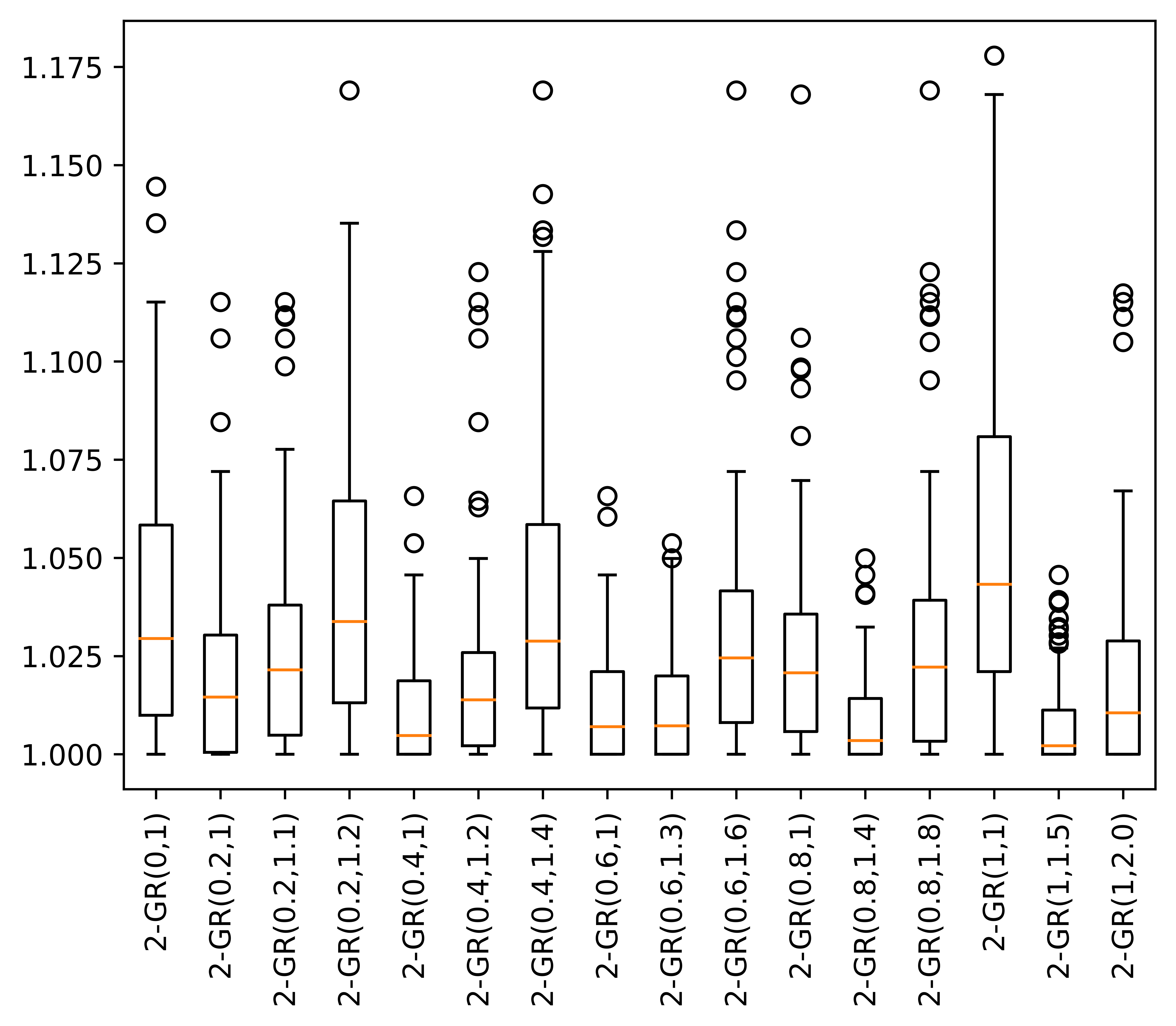
(a)

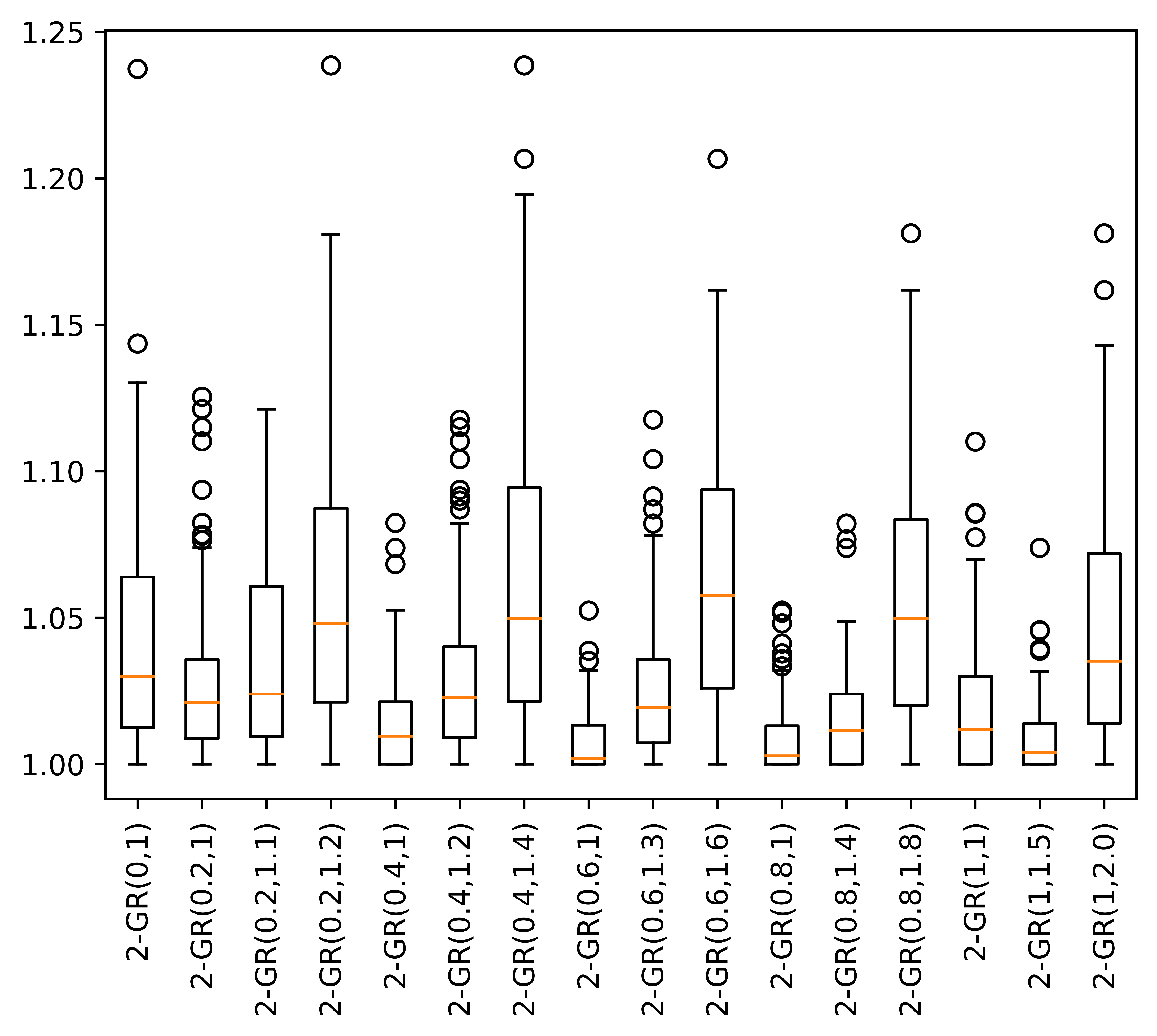
(b)

Figure 3: “Box and whisker” plots to compare $\texttt{2-GR}(\gamma,\eta)$ with different $(\gamma,\eta)\in\texttt{Param}$ in terms of the normalized performance in Section 5.1.

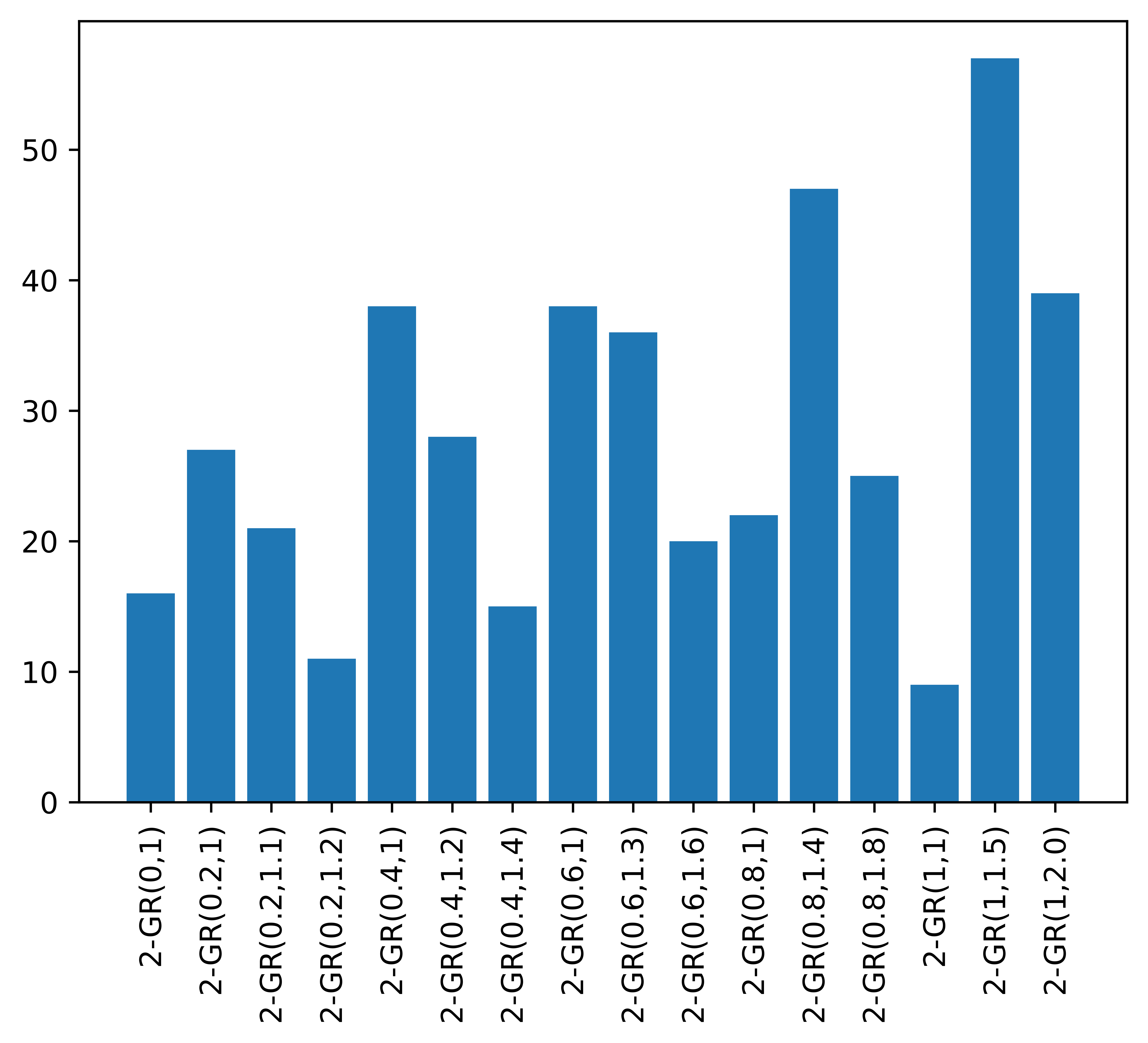
(a)

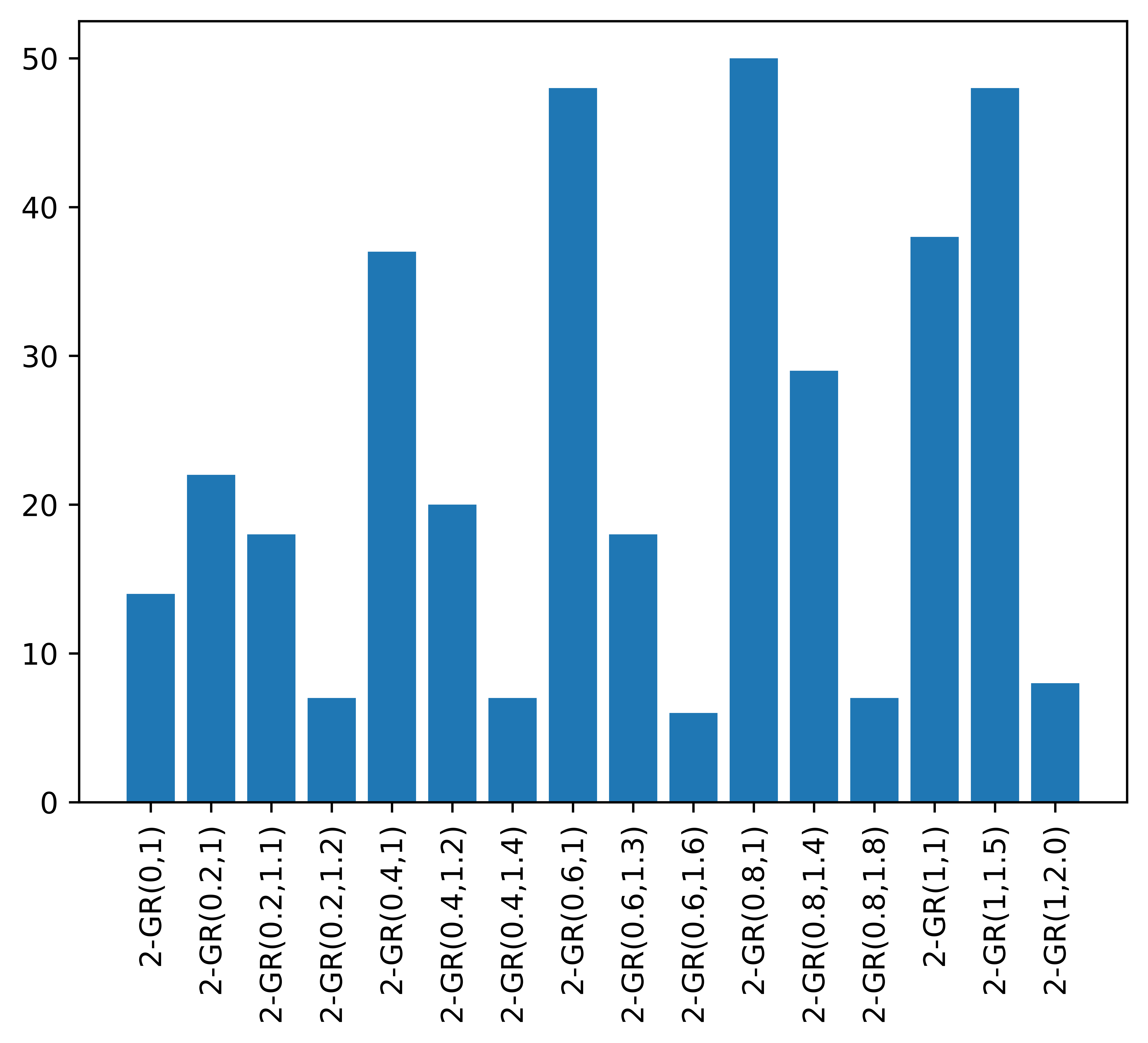
(b)

Figure 4: The frequency that each $(\gamma,\eta)\in\texttt{Param}$ achieves minimum cost among all $\texttt{2-GR}(\gamma,\eta)$) in Section 5.1.

The performance of the 2-Chance Greedy $\texttt{2-GR}(\gamma,\eta)$ with different parameters $(\gamma,\eta)$ In Section 4, we obtain the main theoretical result, i.e., the approximation ratio of 2.497 for the 2-Chance Greedy Algorithm, by considering discount factor $\gamma=1$ and opening cost scalar $\eta=2$. However, for a particular instance, using $\gamma=1$ and $\eta=2$ may not minimize the cost among all $(\gamma,\eta)$ assignments. In practice, the social planner can implement the 2-Chance Greedy Algorithm by varying $(\gamma,\eta)$ and then select the solution with the minimum cost. From Figure 3, we observe that the best average normalized performance among all $\texttt{2-GR}(\gamma,\eta)$ is obtained under $(\gamma=1,\eta=1.5)$ and $(\gamma=0.6,\eta=1)$ for different experiment setups, respectively. In Figure 4, we also plot the frequency that each $(\gamma,\eta)\in\texttt{Param}$ achieves minimum cost among all $\texttt{2-GR}(\gamma,\eta)$.

The impact of discount factor $\gamma$ and opening cost scalar $\eta$ in $\texttt{2-GR}(\gamma,\eta)$ Recall that the approximation ratio of the 2-Chance Greedy Algorithm becomes $\Omega(\log n)$ when discount factor $\gamma$ approaches zero (Example 3.2), while the approximation is constant with positive constant discount factor $\gamma$, e.g., a 2.497-approximation for $\gamma=1,\eta=2$ (Propositions 4.2 and 4.4). From Figure 3, it can be observed that when we fix $\eta=1$, the average normalized performance of $\texttt{2-GR}(\gamma,1)$ is first decreasing and then increasing for $\gamma\in\{0,0.2,0.4,0.6,0.8,1\}$. To understand this behavior, note that the discount factor $\gamma$ controls the impacts of partially connected edges for opening a new facility. Loosely speaking, $\texttt{2-GR}(\gamma,\eta)$ with larger discount factor $\gamma$ opens facilities more aggressively (see Figure 5), and some of those facilities are unnecessary (i.e., removing some facilities from the final solution reduces the total cost). On the other direction, since opening cost scalar $\eta$ controls the tradeoff between the facility opening cost and individual connection cost, the number of opened facilities decreases (and thus less facility opening cost occurs) when we increase opening cost scalar $\eta$ while holding discount factor $\gamma$ fixed.

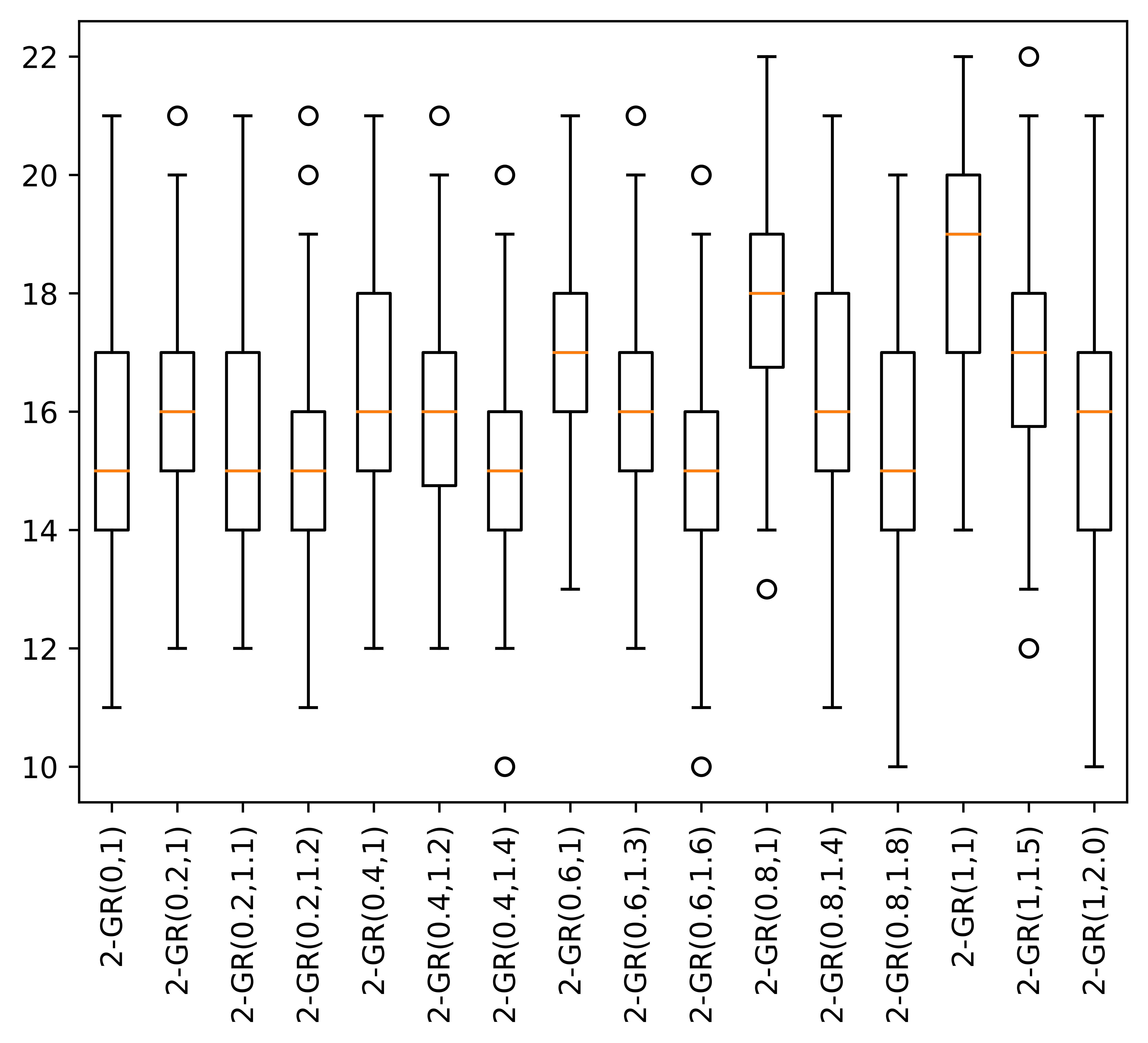
(a)

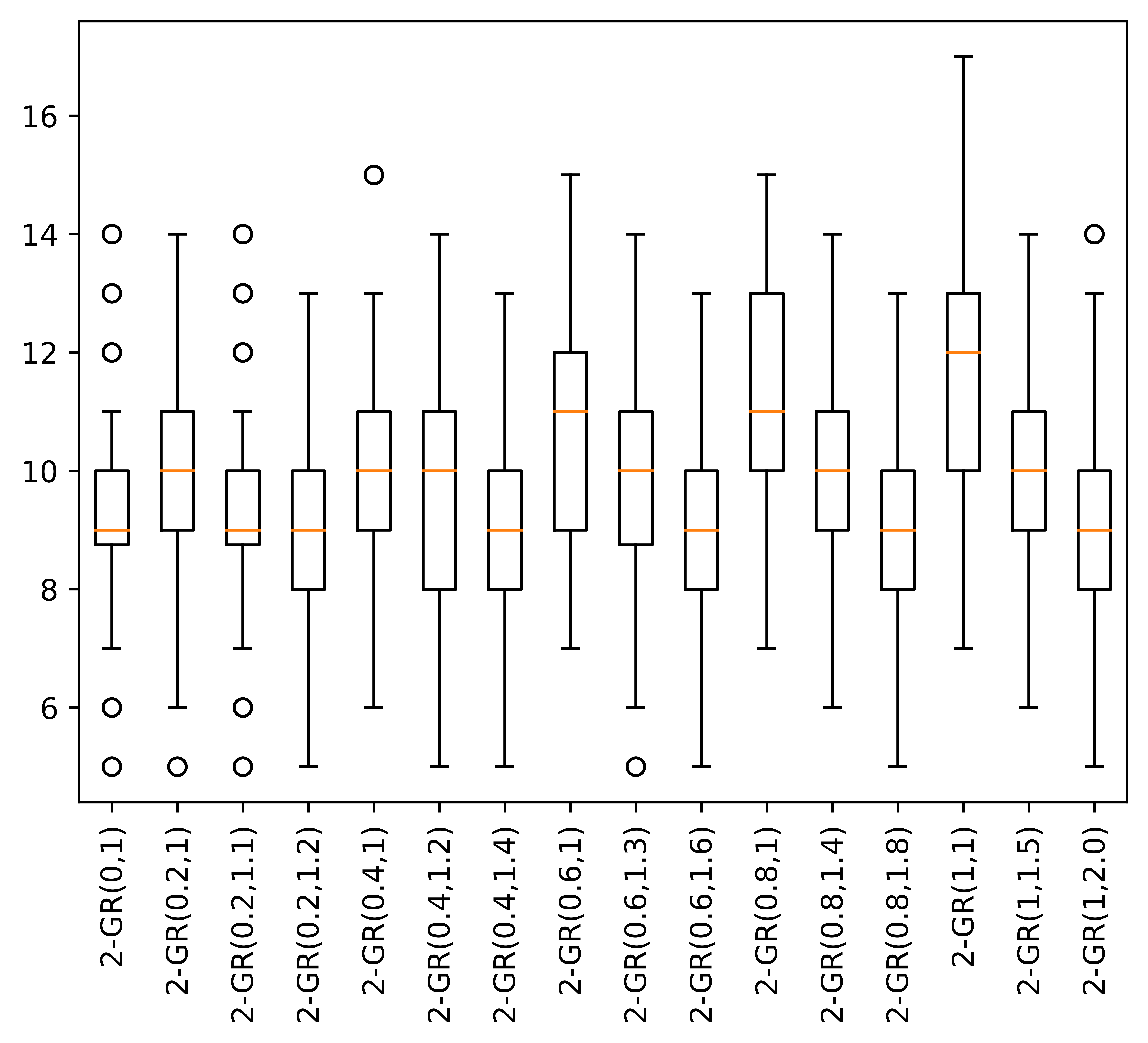
(b)

Figure 5: “Box and whisker” plots to compare $\texttt{2-GR}(\gamma,\eta)$ with different $(\gamma,\eta)\in\texttt{Param}$ in terms of the size of solutions in Section 5.1.

The observation that the 2-Chance Greedy Algorithm might open some unnecessary facilities in fact motivates the 2-Chance Greedy Algorithm with Myopic Pruning ($\texttt{2-GRP}(\gamma,\eta)$) described above. From Table 1, we observe that the average normalized performance of $\texttt{2-GRP}^{*}$ slightly improves. Moreover, $\texttt{2-GRP}^{*}$ not only outperforms all other policies on average, but also beats them in 66 (resp. 73) out of 100 instances under the experiment setup $\bar{f}=20$ (resp. $\bar{f}=100$).

The value of mobility data. When the mobility data $\{\tau_{ij}\}$ is not available and the social planner only has the population (resp. employment) information in each location, one natural heuristic policy is pretending that each individual can only be connected through her home (resp. work) location and then implement GR-H (resp. GR-W). It is clear from Table 1 that both $\texttt{2-GR}^{*}$ and $\texttt{2-GRP}^{*}$ perform noticeably better than GR-H and GR-W. Specifically, the average performance gap between $\texttt{2-GRP}(1)$ and GR-H (resp. GR-W) is 28.4%, 14.1% (resp. 27.7%, 14.1%), respectively. Such performance gap highlights the value of mobility data $\{\tau_{ij}\}$ in this numerical experiment over synthetic data.

5.2 Experiments over US census data

Our second numerical experiment is constructed through US census data.

Experimental setup.

We construct four sets of 2-LFLP instances for four cities in the US, including New York City (NYC), Los Angeles metropolitan area (greater LA), Washington metropolitan area (greater DC), and Raleigh-Durham-Cary CSA (Research Triangle).

In each instance, a location corresponds to a Zip Code Tabulation Area (ZCTA). For each pair of locations, we define their distance as the Euclidean distance between the centroids of their corresponding ZCTAs. We set the facility opening cost $f_{i}$ for each location $i$ as

$$f_{i}\triangleq\bar{f}\cdot z_{i}$$

where $z_{i}$ is the Zillow Home Value Index recorded in Zillow (2022), and $\bar{f}$ is a cost normalization parameter which controls the tradeoff between facility opening costs and individual connection cost in our experiments. Our results are presented for different values of $\bar{f}$.

Finally, US Census Bureau (2019) records the total number of individuals who reside in one census block (CB) and work in another. Aggregating it at the ZCTA level, we complete the construction of $\{\tau_{ij}\}$. We summarize the number of locations and individuals in Table 2.

Table 2: The number of locations and individuals in Section 5.2.

	NYC	greater LA	greater DC	Research Tri.
total locations	177	386	313	102
total population	3166075	5338918	1934411	771249

Policies.

In this numerical experiment, we consider the same set of policies as in Section 5.1: $\texttt{2-GR}(0,1)$ (i.e., JMMSV algorithm) $\texttt{2-GR}^{*}$, $\texttt{2-GRP}^{*}$, GR-H, and GR-W.

Results.

For each city, we construct the 2-LFLP instances under different values of cost normalization parameter $\bar{f}$. Loosely speaking, as parameter $\bar{f}$ increases, the magnitude of facility opening cost increases and consequently the sizes of solutions in all policies decreases. We consider two regimes: low $\bar{f}$ regime (resp. high $\bar{f}$ regime) such that the facilities are opened in 40% to 80% (resp. 5% to 30%) of total locations in policy $\texttt{2-GRP}(1,1)$. For each city and each regime, our results are qualitatively similar. Table 3 and Table 4 illustrate the average normalized performance of different policies for each city in the low $\bar{f}$ regime and the high $\bar{f}$ regime, respectively. Similar to the experiments over synthetic data in Section 5.1, the normalized performance of a policy is defined as the ratio between the cost of this policy and the cost of policy $\texttt{2-GRP}^{*}$. Below we discuss our numerical results in detail.

Table 3: The average normalized (by $\texttt{2-GRP}^{*}$) performance in the low $\bar{f}$ regime.

	$\texttt{2-GR}(0,1)$	$\texttt{2-GR}^{*}$	GR-H	GR-W
NYC	1.041	1.005	1.23	1.1
greater LA	1.018	1.009	1.244	1.096
greater DC	1.003	1.002	1.37	1.094
Research Tri.	1.006	1.001	1.278	1.126

Table 4: The average normalized (by $\texttt{2-GRP}^{*}$) performance in the high $\bar{f}$ regime.

	$\texttt{2-GR}(0,1)$	$\texttt{2-GR}^{*}$	GR-H	GR-W
NYC	1.071	1.003	1.147	1.031
greater LA	1.045	1.01	1.131	1.035
greater DC	1.031	1.008	1.258	1.042
Research Tri.	1.053	1.008	1.223	1.065

JMMSV algorithm vs. 2-Chance Greedy Algorithm. Similar to the observation in Section 5.1, the 2-Chance Greedy Algorithm $\texttt{2-GR}(\gamma,\eta)$ may open some unnecessary facilities and thus $\texttt{2-GRP}(\gamma,\eta)$ using myopic pruning as a post-processing step reduces the cost. Nonetheless, it can be observed in Tables 3 and 4 that such cost reduction is marginal (i.e., less than 1%). On the other hand, there is a performance gap between $\texttt{2-GR}^{*}$ (and thus $\texttt{2-GRP}^{*}$) with the JMMSV algorithm (i.e., $\texttt{2-GR}(0,1)$). For NYC, the gap is 4.1% (7.1%) in the low (high) $\bar{f}$ regime. For the other three cities, in the high $\bar{f}$ regime, the gap is 4.5%, 3.1% and 5.3%, respectively.

The value of mobility data. Similar to the observation in Section 5.2, $\texttt{2-GR}^{*}$ (and thus $\texttt{2-GRP}^{*}$) outperforms GR-H and GR-W for all four cities in both regimes. In the low $\bar{f}$ regime, the performance gap between $\texttt{2-GRP}^{*}$ and $\texttt{GR-H},\texttt{GR-W}$ is more than 23%, 9.4%, respectively (Table 3). In the high $\bar{f}$ regime, the performance gap between $\texttt{2-GRP}^{*}$ and GR-H is still more than 13.1%, but the performance gap between $\texttt{2-GRP}^{*}$ and GR-W becomes 3.1% to 6.5%. (Table 4). Overall our results indicate that in the absence of mobility data, facility placements based on work locations may make sense. However, the value of mobility data is nontrivial in practical settings, and there is significant gain (3-23% based on assumed parameters) for firms for acquiring and leveraging mobility data in their facility location decisions.

6 Conclusion and Future Directions

Motivated by practical applications that utilize mobility data, in this paper, we introduced the 2-location facility location problem. We illustrate the shortcomings of the classic greedy algorithm for facility location in our setup and the APX-hardness of computing the optimal solution. As the main algorithmic contribution of the paper, we propose the 2-Chance Greedy Algorithm. By first conducting a primal-dual analysis and then introducing the strongly factor-revealing quadratic program, we prove that the approximation ratio of the 2-Chance Greedy Algorithm is between $2.428$ and 2.497. We believe that our new analysis framework, in particular the solution-dependent batching argument for obtaining the strongly factor-revealing program, might be of independent interest. We also present extensive numerical studies that justify the performance of our proposed algorithm in practically relevant settings and highlight the value of mobility data. Finally, we extend our model, algorithm, and analysis to the $K$-location facility location problem.

Several open questions arise from this work. The first question is to identify the use of mobility data in other operational problems, such as optimizing transportation systems and scheduling on ride-hailing platforms. Second, inspired by our numerical results, one might want to study (and bound) the value of mobility data theoretically. Since collecting mobility data might be costly, is it possible for a social planner to characterize how much mobility data can improve her decision in isolation or in competitive environments? What are the distinguishing features of settings where this value is expected to be large versus small? Third, there is still a gap (i.e., $[2,\text{2.497}]$) for the optimal approximation ratio among polynomial time algorithms for the 2-LFLP. One can investigate if other algorithmic techniques (e.g., myopic pruning introduced in the numerical section) can be used to further reduce or even close the gap. Fourth, the 2-LFLP in this paper assumes that the individual’s connection cost is the minimum distance between any of her locations to the closest facility. One can consider other connection cost models and adapt the machinery and framework we developed to these variants.

Appendix A Connection to Vertex Cover Problem

In the (weighted) vertex cover problem, given a (vertex-weighted) undirected graph, the goal is to find a subset of vertices with minimum size (total weights) such that every edge intersects this subset (i.e., at least one end point is in this subset). Khot and Regev (2008) establish the following hardness result for the vertex cover problem.

Theorem A.1 (Khot and Regev, 2008).

In the vertex cover problem, there exists no polynomial-time with a $2-\epsilon$ approximation guarantee under the unique game conjecture.

It is straightforward to observe that the 2-LFLP generalizes the weighted vertex cover problem. Given an arbitrary instance in weighted vertex cover problem, we can construct an instance in the 2-LFLP as follows. Each vertex is a location, whose facility opening cost equals to the weight of the vertex. The number of individuals between each pair of locations is one if there is an edge between their corresponding vertices, and zero otherwise. The distance between every pair of distinct locations is infinite. Due to this distance construction, in the 2-LFLP instance, it is necessary for any solution with bounded total cost to open a facility at each individual’s home or work location. Therefore, such solution is a valid vertex cover.

In the weighted vertex cover problem, the 2-Chance Greedy Algorithm with discount factor $\gamma=1$ recovers the classic primal-dual algorithm and is a 2-approximation (Vazirani, 2001). We formalize this in the theorem below and present a proof for completeness.

Theorem A.2.

In the weighted vertex cover problem, the approximation ratio of the 2-Chance Greedy Algorithm with discount factor $\gamma=1$ is 2.

Proof.

For each location $i$, let $E_{i}$ denote the subset of edges whose home or work location is $i$, i.e., $E_{i}=\{e\in E:e_{\texttt{H}}=i\lor e_{\texttt{W}}=i\}$. Now consider the same primal-dual analysis framework as the one in Section 4.1. Specifically, given Lemma 4.7, Lemma 4.8 and dual assignment construction (20), it is sufficient to show that for each location $i\in[n]$, $\sum_{e\in E_{i}}\alpha(e)\leq f_{i}$. We prove this by contradiction. Suppose there exists location $i\in[n]$ such that the inequality is violated. Consider the time stamp $t$ when $\sum_{e\in E_{1}}\alpha_{t}(e)=f_{i}$. Here $\alpha_{t}(e)$ is the value of $\alpha(e)$ at time stamp $t$. Since the distance in the vertex cover problem is infinite, no edge $e\in E_{i}$ has been connected through location $i$. Therefore, the condition of Event (b) for opening location $i$ is satisfied in the algorithm, and thus $\alpha(e)$ stops increasing after time stamp $t$ for every edge $e\in E_{1}$. This leads to a contradiction. ∎

Appendix B The JMMSV Algorithm

See Algorithm 2 for a formal description of the JMMSV algorithm.

1

input :  single location facility location problem instance $I=(n,d,\{\tau_{j}\}_{j\in[n]},\{f_{i}\}_{i\in[n]})$

output : subset $\texttt{SOL}\subseteq[n]$ as the locations of opened facilities.

2

3initialize $\texttt{SOL}\leftarrow\emptyset$

4initialize $\alpha(j)\leftarrow 0$ for each location $j\in[n]$

5initialize $U\leftarrow[n]$,

6initialize $\psi(j)\leftarrow\bot$ for each location $j\in[n]$,

7while $U\not=\emptyset$ do

8       increase $\alpha(j)$ by $d\alpha$ for every location $j\in U$

      /* Event (a) */

9      

10      while there exists location $j\in U$ and location $i\in\texttt{SOL}$ s.t. $\alpha(j)=d(j,i)$  do

11            

12            remove location $j$ from $U$, i.e., $U\leftarrow U\backslash\{j\}$

13            connect location $j$ and facility $i$, i.e., $\psi(j)\leftarrow i$

14      

      /* Event (b) */

15      

16      while there exists location $i\not\in\texttt{SOL}$ s.t. $\sum_{j\in U}\tau_{j}\cdot{\left(\alpha(j)-d(j,i)\right)^{+}}=f_{i}$  do

17            

18            

19            add location $i$ into SOL, i.e., $\texttt{SOL}\leftarrow\texttt{SOL}\cup\{i\}$

20            for each location $j\in U$ do

21                  

22                  if $\alpha(j)-d(j,i)\geq 0$ then

23                        

24                        remove location $j$ from $U$, i.e., $U\leftarrow U\backslash\{j\}$

25                        connect location $j$ and facility $i$, i.e., $\psi(j)\leftarrow i$

26                  

27            

28      

return SOL

Algorithm 2 The JMMSV algorithm (Jain et al., 2003)

Appendix C Extensions to $K$-Location Facility Location Problem

The 2-location facility location problem (2-LFLP) admits a natural extension, which we refer as the $K$-location facility location problem ($K$-LFLP). The $K$-LFLP is the same as the 2-LFLP same except that each individual is associated with $K$ locations. In this model, let $E=[n]^{K}$. We use notation $e=(e_{1},\dots,e_{K})\in E$ to denote individuals associated with $K$ locations $e_{1},\dots,e_{K}$, and refer to $e$ as a hyperedge. The distance between a hyperedge $e$ and location $i$ is defined as $d(e,i)=\min_{\texttt{L}\in[K]}d(e_{\texttt{L}},i)$.

The 2-Chance Greedy Algorithm also admits a natural extension, i.e., $K$-Chance Greedy Algorithm where each hyperedge $e$ can be connected $K$ times through each of its $K$ associated locations. Similar to the 2-Chance Greedy Algorithm, the $K$-Chance Greedy Algorithm is also parameterized by a vector of discount factors $1=\gamma_{0}\geq\gamma_{1}\geq\dots\geq\gamma_{K}=0$ and opening cost scalar $\eta\in\mathbb{R}_{+}$. We say a hyperedge $e$ is $k$-partially connected if it has been connected through $k$ associated locations. The discount factor $\gamma_{k}$ control the impact of $k$-partially connected hyperedge for opening a new facility. See Algorithm 3 for a formal description.

1

input : discount factor $1=\gamma_{0}\geq\gamma_{1}\geq\dots\geq\gamma_{K}=0$, opening cost scalar $\eta\in\mathbb{R}_{+}$, $K$-LFLP instance $I=(n,d,\{\tau_{e}\},\{f_{i}\})$

output : subset $\texttt{SOL}\subseteq[n]$ as the locations of opened facilities.

2

3initialize $\texttt{SOL}\leftarrow\emptyset$

4initialize $\alpha(e)\leftarrow 0$ for each hyperedge $e\in E$

5initialize $U\leftarrow E$,

6initialize $\psi(e,\texttt{L})\leftarrow\bot$ for each hyperedge $e\in E$, each $\texttt{L}\in[K]$

7while $U\not=\emptyset$ do

8       increase $\alpha(e)$ by $d\alpha$ for every hyperedge $e\in U$

      /* Event (a) */

9      

10      while there exists hyperedge $e\in U$ and location $i\in\texttt{SOL}$ s.t. $\alpha(e)=d(e,i)$  do

11            

12            remove hyperedge $e$ from $U$, i.e., $U\leftarrow U\backslash\{e\}$

13            for each $\texttt{L}\in[K]$ do

14                   if $\alpha(e)=d(e_{\texttt{L}},i)$ then

15                        

16                        connect hyperedge $e$ and facility $i$ through location $e_{\texttt{L}}$, i.e., $\psi(e,\texttt{L})\leftarrow i$

17                  

18            

19      

      /* Event (b) */

20      

21      while there exists location $i\not\in\texttt{SOL}$ s.t. $\sum\limits_{e\in U}\tau_{e}\cdot{\left(\alpha(e)-d(e,i)\right)^{+}}+\sum\limits_{\vbox{\Let@\restore@math@cr\default@tag\halign{\hfil$\m@th\scriptstyle#$&$\m@th\scriptstyle{}#$\hfil\cr&e\not\in U\crcr}}}\tau_{e}\cdot{\left(\gamma_{\|\psi(e,\cdot)\|_{0}}\cdot\alpha(e)-\min\limits_{\texttt{L}\in[K]:\psi(e,\texttt{L})=\bot}d(e_{\texttt{L}},i)\right)^{+}}=\eta\cdot f_{i}$  do

22            

            /* subscript $\|\psi(e,\cdot)\|_{0}$ is defined as $\|\psi(e,\cdot)\|_{0}\triangleq|\{\texttt{L}\in[K]:\psi(e,\texttt{L})=\bot\}|$ */

23            

24            

25            add location $i$ into SOL, i.e., $\texttt{SOL}\leftarrow\texttt{SOL}\cup\{i\}$

26            for each hyperedge $e\not\in U$ do

27                   for each $\texttt{L}\in[K]$ do

28                        

29                        if $\psi(e,\texttt{L})=\bot$ and $\gamma\cdot\alpha(e)\geq d(e_{\texttt{L}},i)$ then

30                              

31                              connect hyperedge $e$ and facility $i$ through location $e_{\texttt{L}}$, i.e., $\psi(e,\texttt{L})\leftarrow i$

32                        

33                  

34            

35            for each hyperedge $e\in U$ do

36                  

37                  if $\alpha(e)-d(e,i)\geq 0$ then

38                        

39                        remove hyperedge $e$ from $U$, i.e., $U\leftarrow U\backslash\{e\}$

40                        for each $\texttt{L}\in[K]$ do

41                               if $\alpha(e)\geq d(e_{\texttt{L}},i)$ then

42                                    

43                                    connect hyperedge $e$ and facility $i$ through location $e_{\texttt{L}}$, i.e., $\psi(e,\texttt{L})\leftarrow i$

44                              

45                        

46                  

47            

48      

return SOL

Algorithm 3 $K$-Chance Greedy Algorithm

Inspired by the parameter choice of the 2-Chance Greedy Algorithm, in the remaining of this section, we focus on the $K$-Chance Greedy Algorithm with discount factors $\gamma_{0}=\gamma_{1}=\dots\gamma_{K-1}=1$ and opening cost scalar $\eta=K$, and refer it as the Canonical $K$-Chance Greedy Algorithm for simplicity. The main theoretical guarantee of this algorithm is as follows.

Theorem C.1.

In the $K$-LFLP, the approximation ratio of the Canonical $K$-Chance Greedy Algorithm is at most equal to $\Gamma_{\texttt{SFR-K}}(K)$, where

$$\Gamma_{\texttt{SFR-K}}(K)=\inf\limits_{{n}\in\mathbb{N}}\text{\bf OBJ}\!\left[{\text{\ref{eq:relax strongly factor-revealing quadratic program}}}\right]$$

Here 35 is the maximization program parameterized by ${n}\in\mathbb{N}$ defined as follows:

$$\begin{array}[]{clll}\max\limits_{\begin{subarray}{c}{f}\geq 0,\\ \mathbf{q},\bm{{\alpha}},{\mathbf{d}},{\mathbf{c}}\geq\mathbf{0}\end{subarray}}&\displaystyle\sum\nolimits_{a\in[{n}],b\in[a]}{q}(a,b)\cdot{\alpha}(a,b)&&\\ \text{s.t.}&\texttt{(SFR.i)}\text{--}\texttt{(SFR.vii)}~{}~{}\text{with $\gamma=1$ and $\eta=K$}&\end{array}$$ (35)

Remark C.1.

The constraints in program 35 are the same as the constraints in program $\mathcal{P}_{\texttt{SFR}}({n},1,K)$. Furthermore, the objective function in program 35 is a natural extension of the objective function of program $\mathcal{P}_{\texttt{SFR}}({n},1,2)$. Specifically, program $\mathcal{P}_{\texttt{SFR-2}}({n})$ for $K=2$ recovers program $\mathcal{P}_{\texttt{SFR}}({n},1,2)$.

Proof of Theorem C.1.

The analysis follows the same argument as Theorem 4.1 with two modification on (a) the dual assignment construction (20); and (b) the solution construction for Lemma 4.9: Let $E^{(k)}$ be the hyperedge subset where each hyperedge $e\in E^{(k)}$ are connected to $k$ different facilities in the Canonical $K$-Chance Greedy Algorithm. We assume for every hyperedge $e\in E^{(k)}$, $\psi(e,\texttt{L})\in\texttt{SOL}$ for every $\texttt{L}\in[k]$, and $d(e_{\texttt{L}},\psi(e,\texttt{L}))\leq d(e_{\texttt{L}+1},\psi(e,\texttt{L}+1))$ for every $\texttt{L}\in[k-1]$. This is without loss of generality, since the role of $K$ locations of a fixed hyperedge are ex ante symmetric in our model. For each $k\in[K]$ and each hyperedge $e\in E^{(k)}$, we construct the dual assignment as

$$\mu(e)\leftarrow\tau_{e}\cdot\left(\alpha(e)-\frac{1}{k}\left(\sum_{\texttt{L}\in[k]}d(e_{\texttt{L}},\psi(e,\texttt{L}))\right)+d(e_{\texttt{1}},\psi(e,\texttt{1}))\right)$$

Regarding the solution construction for Lemma 4.9 in the $K$-LFLP, we let variable ${c}^{\dagger}(\kappa(e))\leftarrow N\cdot\alpha(e)$ for all hyperedge $e\in\tilde{E}$ and leave all other variables’ construction remaining the same. Since then, all remaining analysis can be extended straightforwardly. We omit them to avoid repetition. ∎

Note that $\text{\bf OBJ}\!\left[{\text{\hyperref@@ii[eq:relax strongly factor-revealing quadratic program]{$\mathcal{P}_{\texttt{SFR-K}}({n})$}}}\right]\leq\frac{K}{K^{\prime}}\text{\bf OBJ}\!\left[{\text{\hyperref@@ii[eq:relax strongly factor-revealing quadratic program]{$\mathcal{P}_{\texttt{SFR-K}^{\prime}}({n})$}}}\right]$ for every $K\geq K^{\prime}$, since any feasible solution $({f},\mathbf{q},\bm{{\alpha}},{\mathbf{d}},{\mathbf{c}})$ of program $\mathcal{P}_{\texttt{SFR-K}}({n})$ can be converted into a feasible solution $({f}^{\prime}\leftarrow{f},\mathbf{q}^{\prime}\leftarrow\mathbf{q},\bm{{\alpha}}^{\prime}\leftarrow\frac{K^{\prime}}{K}\bm{{\alpha}},{\mathbf{d}}^{\prime}\leftarrow\frac{K^{\prime}}{K}{\mathbf{d}},{\mathbf{c}}^{\prime}\leftarrow\frac{K^{\prime}}{K}{\mathbf{c}})$ of the program $\mathcal{P}_{\texttt{SFR-K}^{\prime}}({n})$. Therefore, it suffices to evaluate program 35 for small $K$’s which also provides upperbounds for larger $K$. In particular, we numerically compute $\text{\bf OBJ}\!\left[{\text{\hyperref@@ii[eq:relax strongly factor-revealing quadratic program]{$\mathcal{P}_{\texttt{SFR-K}}(25)$}}}\right]$ for $K=1,\dots,20$ with software Gurobi, and upperbound the approximation ratios of the Canonical $K$-Chance Greedy Algorithm in Table 5.

The linear dependence on $K$ in the approximation guarantee is unavoidable for all polynomial-time algorithms. Similar to our discussion in Appendix A, the $K$-LFLP generalizes the vertex cover problem for $K$-uniform hypergraphs, which is hard to approximate within any constant factor better than $K$ under the unique game conjecture (Khot and Regev, 2008). Observed that $\frac{1}{K}\cdot\text{\bf OBJ}\!\left[{\text{\hyperref@@ii[eq:relax strongly factor-revealing quadratic program]{$\mathcal{P}_{\texttt{SFR-K}}(25)$}}}\right]$ is monotone decreasing in $K$ as expected in Table 5. In fact, we conjecture that $\lim\limits_{K\rightarrow\infty}\lim\limits_{{n}\rightarrow\infty}\frac{1}{K}\cdot\text{\bf OBJ}\!\left[{\text{\ref{eq:relax strongly factor-revealing quadratic program}}}\right]=1$ and thus the Canonical $K$-Chance Greedy Algorithm attains asymptotic optimal approximation ratio of $K+o(1)$ as $K$ becomes large.

Table 5: The approximation ratio upper bounds (UB) of the Canonical $K$-Chance Greedy Algorithm.

$K$	1	2	3	4	5	6	7	8	9	10	11
UB	1.864	2.497	3.538	4.58	5.611	6.659	7.685	8.714	9.769	10.816	11.855
$K$	12	13	14	15	16	17	18	19	20	$\geq 21$
UB	12.887	13.912	14.93	15.941	16.944	18.0	19.059	20.118	21.176	$1.059K$

Appendix D Missing Proofs

D.1 Proof of theorem 4.1

See 4.1

Proof.

Combining Lemma 4.5 and Lemma 4.10 finishes the proof. ∎

D.2 Proof of Proposition 4.4

See 4.4

Proof.

Consider constraint (SFR.iii) at $a=1$,

$$\eta\cdot{f} \geq{q}(2,1)\cdot{\left(\gamma\cdot{\alpha}(2,1)-{d}(2,1)\right)^{+}}+{q}(2,2)\cdot{\left(\gamma\cdot{\alpha}(1,1)-{d}(2,2)\right)^{+}}$$

$$\geq{q}(2,2)\cdot\gamma\cdot{\alpha}(1,1)-{d}(2,2)\overset{(a)}{\geq}\gamma\cdot{\alpha}(1,1)-{d}(2,2)\$$

where inequality (a) holds due to constraint (SFR.vii) at $$b=2$$. Hence,

$${\alpha}(1,1) \leq\frac{1}{\gamma}\cdot\left(\eta\cdot{f}+{d}(2,2)\right)\overset{(a)}{\leq}\frac{\eta}{\gamma}$$

where inequality (a) holds due to constraints (SFR.vi) and (SFR.vii) at $$b=2 a=1,a^{\prime}=2,b=1,b^{\prime}=2$$. Invoking constraint (SFR.ii) at ,

$$\gamma\cdot{\alpha}(2,2) \leq{c}(1,1)+{d}(1,1)+{d}(2,2)\overset{(a)}{\leq}{\alpha}(1,1)+{\alpha}(1,1)+{d}(2,2)\overset{(b)}{\leq}\frac{2\eta}{\gamma}+1\leq\frac{3\eta}{\gamma}$$

where inequality (a) holds due to constraints (SFR.v) and (SFR.iv) at $$a=1,b=1 {\alpha}(1,1)\leq\frac{1}{\gamma} {d}(2,2)\leq 1 b=2$$; and inequality (b) holds since and implied by constraints (SFR.vi) and (SFR.vii) at . Putting all pieces together,

$$~{}~{}~{}~{}\text{\bf OBJ}\!\left[{\text{\hyperref@@ii[eq:strongly factor-revealing quadratic program]{$\mathcal{P}_{\texttt{SFR}}(2,\gamma,\eta)$}}}\right]$$

$$={q}(1,1)\cdot\left(\frac{1+\gamma}{\eta}\cdot{\alpha}(1,1)-\left(\frac{1+\gamma}{\eta}-1\right)\cdot{c}(1,1)\right)$$

$$\qquad+{q}(2,1)\cdot\left(\frac{1+\gamma}{\eta}\cdot{\alpha}(2,1)-\left(\frac{1+\gamma}{\eta}-1\right)\cdot{c}(2,1)\right)$$

$$\qquad+{q}(2,2)\cdot\left(\frac{1+\gamma}{\eta}\cdot{\alpha}(2,2)-\left(\frac{1+\gamma}{\eta}-1\right)\cdot{c}(2,2)\right)$$

$$\leq\frac{1+\gamma}{\eta}\cdot\left({q}(1,1)\cdot{\alpha}(1,1)+{q}(2,1)\cdot{\alpha}(2,1)+{q}(2,2)\cdot{\alpha}(2,2)\right)$$

$$\overset{(a)}{\leq}\frac{1+\gamma}{\eta}\cdot\left({q}(1,1)+{q}(2,1)+{q}(2,2)\right)\cdot{\alpha}(2,2)$$

$$\overset{(b)}{\leq}\frac{1+\gamma}{\eta}\cdot 2\cdot\frac{3\eta}{\gamma^{2}}=\frac{6(1+\gamma)}{\gamma^{2}}$$

where inequality (a) holds due to constraint (SFR.i), and inequality (b) holds since ${\alpha}(2,2)\leq\frac{3\eta}{\gamma^{2}}$ and constraint (SFR.vii). ∎

D.3 Proof of Proposition 4.3

See 4.3

To prove Proposition 4.3, we introduce the following lemma.

Lemma D.1.

There exists a 2-LFLP instance such that the approximation of the 2-Chance Greedy Algorithm with discount factor $\gamma=1$ and opening cost scalar $\eta=2$ is at least equal to $\sup_{{m}\in\mathbb{N}}\text{\bf OBJ}\!\left[{\text{\hyperref@@ii[eq:lower bound LP]{$\mathcal{P}_{\texttt{LB}}({m})$}}}\right]$, where program 42 is the following maximization program parameterized by ${m}\in\mathbb{N}$,

$$\begin{array}[]{llll}\max\limits_{\begin{subarray}{c}{f}\geq 0,\\ \bm{{\alpha}},{\mathbf{d}},{\mathbf{c}}\geq\mathbf{0}\end{subarray}}&\displaystyle\sum\nolimits_{\ell\in[{m}]}{\alpha}(\ell)&\text{s.t.}&\\ &{\alpha}(\ell)\leq{\alpha}(\ell^{\prime})&\ell,\ell^{\prime}\in[{m}],\ell\leq\ell^{\prime}\\ &{\alpha}(\ell^{\prime})\leq{c}(\ell)+{d}(\ell)+{d}(\ell^{\prime})&\ell,\ell^{\prime}\in[{m}],\ell\leq\ell^{\prime}&\\ &{c}(\ell)\leq{\alpha}(\ell)&\ell\in[{m}]\\ &\displaystyle\sum\nolimits_{\ell^{\prime}\in[\ell:{m}]}{\left({\alpha}(\ell)-{d}(\ell^{\prime})\right)^{+}}\leq 2{f}&\ell\in[{m}]\\ &{f}+\displaystyle\sum\nolimits_{\ell\in[{m}]}{d}(\ell)=1&\end{array}$$ (42)

It is worth highlighting that program $\mathcal{P}_{\texttt{SFR}}({m},1,2)$ can be considered as a relaxation of program 42. In particular, from every feasible solution $({f},\{{\alpha}(\ell),{d}(\ell),{c}(\ell)\}_{\ell\in[{m}]})$ of program 42, we can straightforwardly construct a feasible solution $({f}^{\dagger},\{{\alpha}^{\dagger}(a,b),{d}^{\dagger}(a,b),{c}^{\dagger}(a,b),{q}^{\dagger}(a,b)\}_{a\in[{m}],b\in[a]})$ of program $\mathcal{P}_{\texttt{SFR}}({m},1,2)$ as follows,

$${f}^{\dagger}\leftarrow{f},$$

$$a\in[{m}],b\in[a]:\qquad {\alpha}^{\dagger}(a,b)\leftarrow{\alpha}(a),\quad{d}^{\dagger}(a,b)\leftarrow{d}(a),$$

$${c}^{\dagger}(a,b)\leftarrow{c}(a),\quad{q}^{\dagger}(a,b)\leftarrow{\mathbbm{1}\left\{a=b\right\}}$$

and both solutions have the same objective value.

Given Lemma D.1, the proof of Proposition 4.3 is based on the lowerbound of program $\mathcal{P}_{\texttt{LB}}(500)$ numerically computed with software Gurobi.

Proof of Lemma D.1.

Given any feasible solution $({f}^{\dagger},\{{\alpha}^{\dagger}(\ell),{d}^{\dagger}(\ell),{c}^{\dagger}(\ell)\})$ in program 42, we can construct a 2-LFLP instance such that the approximation ratio of the 2-Chance Greedy Algorithm with $\gamma=1$ and $\eta=2$ equals to the objective value of this solution.

Fix an arbitrary small $\epsilon>0$. In this 2-LFLP instance, there are $n\triangleq 4{m}+1$ locations with facility opening cost as follows,

$$f_{i}=\left\{\begin{array}[]{ll}\infty&\quad\forall i\in[2{m}]\\ {\alpha}^{\dagger}(i-2{m})-{c}^{\dagger}(i-2{m})&\quad\forall i\in[2{m}+1:3{m}]\\ {\alpha}^{\dagger}(i-3{m})-{c}^{\dagger}(i-3{m})&\quad\forall i\in[3{m}+1:4{m}]\\ {f}^{\dagger}+\epsilon&\quad~{}~{}i=4{m}+1\end{array}\right.$$

The distance function $d$ satisfies that

$$\forall i\in[{m}]: \qquad d(i,i+2{m})={c}^{\dagger}(i),\quad d(i+{m},i+3{m})={c}^{\dagger}(i),$$

$$\qquad d(i,n)={d}^{\dagger}(i),\quad\quad\quad d(i+{m},n)=\infty$$

and triangle inequality holds with equality for all other pairs of locations.

There are ${m}$ individuals where each individual $i\in[{m}]$ resides at location $i$ and works at location $i+{m}$. Namely, the number of individuals $\{\tau_{e}\}$ are

$$\tau_{e}=\left\{\begin{array}[]{ll}1&\quad\text{if $e_{\texttt{H}}\in[{m}]$ and $e_{\texttt{W}}=e_{\texttt{H}}+{m}$}\\ 0&\quad\text{o.w.}\end{array}\right.$$

The optimal solution opens a facility at location $4{m}+1$ (i.e., $\texttt{OPT}=\{4{m}+1\}$ with optimal total cost $\text{\bf COST}\!\left[{\texttt{OPT}}\right]=f^{\dagger}+\epsilon+\sum_{i\in[{m}]}{d}^{\dagger}(i)=1+\epsilon$.

In contrast, consider the 2-Chance Greedy Algorithm with $\gamma=1$ and $\eta=2$. At time stamp ${\alpha}^{\dagger}(1)$, the conditions of Event (b) for opening facility $2{m}+1$ and facility $3{m}+1$ are satisfied due to individual $1$ who resides at location $i$ and works at location ${m}+1$. Thus, the algorithm opens both facility $2{m}+1$ and facility $3{m}+1$, and fully connects individual 1 to those two facilities through her home $1$ and work location $1+{m}$, respectively. Then at time stamp ${\alpha}^{\dagger}(2)$, facilities at location $2{m}+2$ and $3{m}+2$ are opened due to individual $2$. Proceeding similarly, it can be seen that when the algorithm terminates, it outputs $\texttt{SOL}=\{2{m}+1,\dots,4{m}\}$ with total cost $\text{\bf COST}\!\left[{\texttt{SOL}}\right]=\sum_{i\in[{m}]}2{\alpha}^{\dagger}(i)-{c}^{\dagger}(i)\geq\sum_{i\in[{m}]}{\alpha}^{\dagger}(i)$.

Putting all pieces together, as $\epsilon$ goes to zero, the approximation of the 2-Chance Greedy Algorithm with $\gamma=1$ and $\eta=2$ converges to the objective value of solution $({f}^{\dagger},\{{\alpha}^{\dagger}(\ell),{d}^{\dagger}(\ell),{c}^{\dagger}(\ell)\})$ as desired. ∎

D.4 Proof of Lemma 4.6

See 4.6

Proof.

We first show property (i). By definition of $\mathcal{Y}$, if $\mathcal{Y}(e,\texttt{L})<\mathcal{Y}(e^{\prime},\texttt{L}^{\prime})$, edge $e$ is connected through home/work location $e_{\texttt{L}}$ before the termination of the algorithm, and thus $\psi(e,\texttt{L})\not=\bot$. At time stamp $\mathcal{Y}(e,\texttt{L})$, facility $\psi(e,\texttt{L})$ has been opened, and edge $e^{\prime}$ has not been connected through its home/work location $e^{\prime}_{\texttt{L}^{\prime}}$ yet. This implies that $\gamma\cdot\alpha(e^{\prime})<d(e^{\prime}_{\texttt{L}^{\prime}},\psi(e,\texttt{L}))$. Otherwise, the condition of Event (a) is satisfied, i.e., edge $e^{\prime}$ should be connected to facility $\psi(e,\texttt{L})$ through its home/work location $e^{\prime}_{\texttt{L}^{\prime}}$ weakly before time stamp $\mathcal{Y}(e,\texttt{L})$, which is a contradiction. Therefore,

$$\gamma\cdot\alpha(e^{\prime})<d(e^{\prime}_{\texttt{L}^{\prime}},\psi(e,\texttt{L}))\overset{}{\leq}d(e_{\texttt{L}},\psi(e,\texttt{L}))+d(e_{\texttt{L}},i)+d(e^{\prime}_{\texttt{L}^{\prime}},i)$$

where the second inequality holds due to the triangle inequality.

Next we prove property (ii) by contradiction. Suppose there exists a location $i\in[n]$ and edge $e\in E$ such that

$$\sum_{e^{\prime}\in E:\mathcal{Y}(e^{\prime},\sigma_{i}(e^{\prime}))\geq\mathcal{Y}(e,\sigma_{i}(e))}{\left(\gamma\cdot\min\left\{\alpha(e),\alpha(e^{\prime})\right\}-d(e^{\prime}_{\sigma_{i}(e^{\prime})},i)\right)^{+}}>\eta\cdot f_{i}$$

Now consider the algorithm at time stamp $t\triangleq\mathcal{Y}(e,\sigma_{i}(e))-\epsilon$ for sufficiently small $\epsilon$. By definition, none of edges $e^{\prime}\in E$ with $\mathcal{Y}(e^{\prime},\sigma_{i}(e^{\prime}))\geq\mathcal{Y}(e,\sigma_{i}(e))$ has been connected to any facility through its home/work location $e^{\prime}_{\sigma_{i}(e^{\prime})}$. In a slight abuse of notation, let $\alpha_{t}(e^{\prime})$ be the value of variable $\alpha(e^{\prime})$ in the algorithm at time stamp $t$. By construction, we know that $\alpha_{t}(e^{\prime})\geq\min\{t,\alpha(e^{\prime})\}$, and $t\geq\alpha(e)$. Thus, we claim that facility $i$ is opened weakly before time stamp $t$, since the condition of Event (b) for opening facility $i$ is satisfied at time stamp $t$. Moreover, there exists at least an edge $e^{\prime}\in E$ such that $\mathcal{Y}(e^{\prime},\sigma_{i}(e^{\prime}))\geq t$ and $\gamma\cdot\alpha_{t}(e^{\prime})\geq d(e^{\prime}_{\sigma_{i}(e^{\prime})},i)$. This implies that edge $e^{\prime}$ is connected to facility $i$ through its $e^{\prime}_{\sigma_{i}(e^{\prime})}$ weakly before time stamp $t$, which is a contradiction.

Finally, property (iii) is guaranteed by the construction of the algorithm, and the assumption that $\gamma\in[0,1]$. ∎

D.5 Proof of Lemma 4.7

See 4.7

Proof.

Consider the following integer solution of program 19. For each service configuration $S=(i,\tilde{E})$, set $x(S)=1$ if the optimal solution OPT opens facility $i$ and serves all edges in $\tilde{E}$ through facility $i$; and $x(S)=0$ otherwise. It can be verified that this solution is feasible and its objective value equals the optimal cost $\text{\bf COST}\!\left[{\texttt{OPT}}\right]$. Therefore, $\text{\bf COST}\!\left[{\texttt{OPT}}\right]\geq\text{\bf OBJ}\!\left[{\text{\ref{eq:lp relaxtion}}}\right]$. ∎

D.6 Proof of Lemma 4.8

See 4.8

Proof.

By the dual assignment (20), we have

$$\sum_{e\in E}\mu(e)= \sum_{e\in E^{(1)}}\tau_{e}\cdot\left(\frac{1+\gamma}{\eta}\cdot\alpha(e)-\left(\frac{1+\gamma}{\eta}-1\right)\cdot d(e_{\texttt{H}},\psi(e,\texttt{H}))\right)$$

$$\quad+\sum_{e\in E^{(2)}}\tau_{e}\cdot\left(\frac{1+\gamma}{\eta}\cdot\alpha(e)-\frac{1}{\eta}\left(d(e_{\texttt{H}},\psi(e,\texttt{H}))+d(e_{\texttt{W}},\psi(e,\texttt{W}))\right)+d(e_{\texttt{H}},\psi(e,\texttt{H}))\right)$$

We analyze the term of each individual on each edge $e$ on the right-hand side separately. For each individual on edge $e\in E^{(1)}$, we have

$$~{}\frac{1+\gamma}{\eta}\cdot\alpha(e)-\left(\frac{1+\gamma}{\eta}-1\right)\cdot d(e_{\texttt{H}},\psi(e,\texttt{H}))$$

$$= ~{}\frac{1+\gamma}{\eta}\cdot\left(\alpha(e)-d(e_{\texttt{H}},\psi(e,\texttt{H}))\right)+d(e_{\texttt{H}},\psi(e,\texttt{H}))$$

$$\geq ~{}\frac{1}{\eta}\cdot\left(\alpha(e)-d(e_{\texttt{H}},\psi(e,\texttt{H}))\right)+d(e_{\texttt{H}},\psi(e,\texttt{H}))$$

where the last inequality holds since $\alpha(e)\geq d(e_{\texttt{H}},\psi(e,\texttt{H}))$, which is implied by the construction of the 2-Chance Greedy Algorithm.

For each individual on edge $e\in E^{(2)}$, we have

$$~{}\frac{1+\gamma}{\eta}\cdot\alpha(e)-\frac{1}{\eta}\left(d(e_{\texttt{H}},\psi(e,\texttt{H}))+d(e_{\texttt{W}},\psi(e,\texttt{W}))\right)+d(e_{\texttt{H}},\psi(e,\texttt{H}))$$

$$= ~{}\frac{1}{\eta}\cdot\left((1+\gamma)\alpha(e)-d(e_{\texttt{H}},\psi(e,\texttt{H}))-d(e_{\texttt{W}},\psi(e,\texttt{W}))\right)+d(e_{\texttt{H}},\psi(e,\texttt{H}))$$

Combining two pieces together, we obtain

$$\sum_{e\in E}\mu(e) \geq\frac{1}{\eta}\cdot\left(\sum_{e\in E^{(1)}}\tau_{e}\cdot\left(\alpha(e)-d(e_{\texttt{H}},\psi(e,\texttt{H}))\right)+\sum_{e\in E^{(2)}}\tau_{e}\cdot\left((1+\gamma)\alpha(e)-d(e_{\texttt{H}},\psi(e,\texttt{H}))-d(e_{\texttt{W}},\psi(e,\texttt{W}))\right)\right)$$

$$\qquad+\sum_{e\in E}\tau_{e}\cdot d(e_{\texttt{H}},\psi(e,\texttt{H}))$$

To finish the proof, note that the construction (i.e., the condition of Event (b)) of the 2-Chance Greedy Algorithm implies that the first term on the right-hand side is equal to the facility opening cost of solution SOL, and the second term on the right-hand side is at least the connection cost of solution SOL. ∎

D.7 Proof of Lemma 4.9

See 4.9

Proof.

Fix an arbitrary 2-LFLP instance, and an arbitrary service region $S=(i,\tilde{E})\in\mathcal{S}$ such that $f_{i}+\sum_{e\in\tilde{E}}d(e,i)>0$. We construct a solution $\{{f}^{\dagger},{\alpha}^{\dagger}(\ell),{d}^{\dagger}(\ell),{c}^{\dagger}(\ell)\}$ for program 16 as follows:

$$\qquad{f}^{\dagger}\leftarrow N\cdot{f_{i}},$$

$$e\in\tilde{E}: \qquad{\alpha}^{\dagger}(\kappa(e))\leftarrow N\cdot{\alpha(e)},\quad{d}^{\dagger}(\kappa(e))\leftarrow N\cdot{d(e,i)},$$

$$e\in\tilde{E}\cap E^{(1)}: \qquad{c}^{\dagger}(\kappa(e))\leftarrow{d}(e_{\texttt{H}},\psi(e,\texttt{H})),$$

$$e\in\tilde{E}\cap E^{(2)}: \qquad{c}^{\dagger}(\kappa(e))\leftarrow N\cdot d(e_{\sigma_{i}(e)},\psi(e,\sigma_{i}(e)))$$

where $N=\frac{1}{f_{i}+\sum_{e\in\tilde{E}}d(e,i)}$ is the normalization factor which guarantees the feasibility of constraint (FR.iv). Moreover, Lemma 4.6 and the solution construction implies the feasibility of constraints (FR.i), (FR.ii), and (FR.iii).

Finally, we argue that $\frac{\sum_{e\in\tilde{E}}\mu(e)}{c(S)}$ is upperbounded by the objective value of the constructed solution in program 16. It is sufficient to show that for every edge $e\in\tilde{E}$,

$$\frac{\mu(e)}{c(S)}\leq\frac{1+\gamma}{\eta}\cdot{\alpha}^{\dagger}(\kappa(e))-\left(\frac{1+\gamma}{\eta}-1\right)\cdot{c}^{\dagger}(\kappa(e))$$

We show this inequality for two different cases separately.

For each edge $e\in\tilde{E}\cap E^{(1)}$, we have

$$\frac{\mu(e)}{c(S)} \overset{(a)}{=}\frac{\frac{1+\gamma}{\eta}\cdot\alpha(e)-\left(\frac{1+\gamma}{\eta}-1\right)\cdot d(e_{\texttt{H}},\psi(e,\texttt{H}))}{{}f_{i}+\sum_{e^{\prime}\in\tilde{E}}d(e^{\prime},i)}$$

$$\overset{(b)}{=}\frac{\frac{1+\gamma}{\eta}\cdot{\alpha}^{\dagger}(\kappa(e))-\left(\frac{1+\gamma}{\eta}-1\right)\cdot{c}^{\dagger}(\kappa(e))}{{}f^{\dagger}+\sum_{\ell\in[m]}d^{\dagger}(\ell)}$$

$$\overset{(c)}{\leq}\frac{1+\gamma}{\eta}\cdot{\alpha}^{\dagger}(\kappa(e))-\left(\frac{1+\gamma}{\eta}-1\right)\cdot{c}^{\dagger}(\kappa(e))$$

where equality (a) holds due to $\tau_{e}=1$ and the dual assignment (20); equality (b) holds due to the solution construction in program 16; and inequality (c) holds due to constraint (FR.iv) in program 16.

For each edge $e\in\tilde{E}\cap E^{(2)}$, we have

$$\frac{\mu(e)}{c(S)} \overset{(a)}{=}\frac{\frac{1+\gamma}{\eta}\cdot\alpha(e)-\frac{1}{\eta}\left(d(e_{\texttt{H}},\psi(e,\texttt{H}))+d(e_{\texttt{W}},\psi(e,\texttt{W}))\right)+d(e_{\texttt{H}},\psi(e,\texttt{H}))}{f_{i}+\sum_{e^{\prime}\in\tilde{E}}d(e^{\prime},i)}$$

$$\overset{}{=}\frac{\frac{1+\gamma}{\eta}\cdot\alpha(e)-\frac{1}{\eta}d(e_{\texttt{W}},\psi(e,\texttt{W}))+\left(1-\frac{1}{\eta}\right)d(e_{\texttt{H}},\psi(e,\texttt{H}))}{f_{i}+\sum_{e^{\prime}\in\tilde{E}}d(e^{\prime},i)}$$

$$\overset{(b)}{\leq}\frac{\frac{1+\gamma}{\eta}\cdot\alpha(e)-\frac{1}{\eta}d(e_{\texttt{W}},\psi(e,\texttt{W}))+\left(1-\frac{1}{\eta}\right)d(e_{\texttt{W}},\psi(e,\texttt{W}))}{f_{i}+\sum_{e^{\prime}\in\tilde{E}}d(e^{\prime},i)}$$

$$\overset{(c)}{\leq}\frac{\left(\frac{1+\gamma}{\eta}\cdot{\alpha}^{\dagger}(\kappa(e))-\left(\frac{1+\gamma}{\eta}-1\right)\cdot{c}^{\dagger}(\kappa(e))\right)}{f^{\dagger}+\sum_{\ell\in[m]}d^{\dagger}(\ell)}$$

$$\overset{(d)}{\leq}\frac{1+\gamma}{\eta}\cdot{\alpha}^{\dagger}(\kappa(e))-\left(\frac{1+\gamma}{\eta}-1\right)\cdot{c}^{\dagger}(\kappa(e))$$

where equality (a) holds due to $\tau_{e}=1$ and the dual assignment (20); inequality (b) holds due to the assumption that $d(e_{\texttt{H}},\psi(e,\texttt{H}))\leq d(e_{\texttt{W}},\psi(e,\texttt{W}))$ introduced in step 2 and $(1-\nicefrac{{1}}{{\eta}})\geq 0$; equality (c) holds due to the solution construction in program 16, the assumption that $d(e_{\texttt{H}},\psi(e,\texttt{H}))\leq d(e_{\texttt{W}},\psi(e,\texttt{W}))$ introduced in step 2 and $\nicefrac{{2}}{{\eta}}-1\geq\nicefrac{{(1+\gamma)}}{{\eta}}-1\geq 0$; and inequality (d) holds due to constraint (FR.iv) in program 16. ∎

D.8 Proof of Lemma 4.10

See 4.10

Before the proof of Lemma 4.10, we first present a technical lemma as follows.

Lemma D.2.

For any $\gamma\in[0,1],~{}{m}\in\mathbb{N},~{}\chi:[{m}]\rightarrow\tiny\mathbb{R}_{+}$ and any feasible solution $({f},\{{\alpha}(\ell),{d}(\ell),{c}(\ell)\})$ of program 16, there exists ${m}^{\dagger}\in\mathbb{N},~{}\chi^{\dagger}:[{m}^{\dagger}]\rightarrow\tiny\mathbb{R}_{+}$ and a feasible solution $({f}^{\dagger},\{{\alpha}^{\dagger}(\ell),{d}^{\dagger}(\ell),{c}^{\dagger}(\ell)\})$ of program $\mathcal{P}_{\texttt{FR}}({m}^{\dagger},\chi^{\dagger},\gamma)$ such that ${d}^{\dagger}(\ell)\leq{\alpha}^{\dagger}(\ell)$ for every $\ell\in[{m}^{\dagger}]$ and has weakly higher objective value.

Proof.

Let $\ell^{*}$ be the index with largest ${\alpha}(\ell)$, i.e., $\ell^{*}=\mathop{\mathrm{arg\,max}}_{\ell\in[{m}]}{\alpha}(\ell)$. If ${d}(\ell^{*})>{\alpha}(\ell^{*})$, then we can update ${\alpha}(\ell^{*})\leftarrow{d}(\ell^{*})$. It can be verified that the updated solution is still feasible in program 16 (in particular, constraints (FR.i)and (FR.ii) are still satisfied), and has higher objective value.

Now, we partition index set $[{m}]$ into two subsets: $\Delta=\{\ell\in[{\alpha}]:{d}(\ell)\leq{\alpha}(\ell)\}$ and $\bar{\Delta}=[{m}]\backslash\Delta$. As we discussed in the previous paragraph, $\ell^{*}\in\Delta$. Let $g$ be an arbitrary bijection from $\Delta$ to $[|\Delta|]$. Consider the following construction of parameters ${m}^{\dagger},\chi^{\dagger}$:

$$\qquad{m}^{\dagger}\leftarrow|\Delta|,$$

$$\ell\in\Delta: \qquad\chi^{\dagger}(g(\ell))\leftarrow\chi(\ell),$$

and solution $$({f}^{\dagger},\{{\alpha}^{\dagger}(\ell),{d}^{\dagger}(\ell),{c}^{\dagger}(\ell)\})$$:

$$\qquad{f}^{\dagger}\leftarrow{f},$$

$$\qquad{\alpha}^{\dagger}(g(\ell^{*}))\leftarrow{\alpha}(\ell^{*})+\sum_{\ell\in\bar{\Delta}}{d}(\ell),\quad{d}^{\dagger}(g(\ell^{*}))\leftarrow{d}(\ell^{*})+\sum_{\ell\in\bar{\Delta}}{d}(\ell),\quad{c}^{\dagger}(g(\ell^{*}))\leftarrow{c}(\ell^{*})$$

$$\ell\in\Delta\backslash\{\ell^{*}\}: \qquad{\alpha}^{\dagger}(g(\ell))\leftarrow{\alpha}(\ell),\quad{d}^{\dagger}(g(\ell))\leftarrow{d}(\ell),\quad{c}^{\dagger}(g(\ell))\leftarrow{c}(\ell)$$

It is straightforward to verify that the constructed solution is feasible in program $\mathcal{P}_{\texttt{FR}}({m}^{\dagger},\chi^{\dagger},\gamma)$, and has weakly higher objective value. ∎

Now we are ready to present the proof of Lemma 4.10.

Proof of Lemma 4.10.

Fix an arbitrary $\gamma\in[0,1],~{}{n}\in\mathbb{N},~{}{m}\in\mathbb{N}$ and $\chi:[{m}]\rightarrow$. Consider an arbitrary feasible solution feasible solution $({f},\{{\alpha}(\ell),{d}(\ell),{c}(\ell)\})$ of program 16 such that ${d}(\ell)\leq{\alpha}(\ell)$ for each $\ell\in[{m}]$. It is sufficient for us to construct a feasible solution $({f},\{{q}(a,b),{\alpha}(a,b),{d}(a,b),{c}(a,b)\})$ of program 10 with weakly higher objective value. Our argument proceeds in four steps as we sketched in Section 4.2.2.

Step 1- identifying pivotal index subset $L$ with monotone ${\alpha}(\ell)$.

Consider a sequence of $k$ indexes $\ell_{1}<\ell_{2}<\dots<\ell_{k}$ for some $k\in\mathbb{N}$ such that

$$\forall\ell\in[{m}]: \qquad\chi(\ell_{1})\leq\chi(\ell)$$

$$\forall a\in[k-1]: \qquad\chi(\ell_{a})<\chi(\ell_{a+1})$$

$$\forall a\in[k-1]: \qquad{\alpha}(\ell_{a})<{\alpha}(\ell_{a+1})$$

$$\forall a\in[k],~{}\forall\ell\in\{\ell^{\prime}\in[{m}]:\chi(\ell_{a})\leq\chi(\ell^{\prime})<\chi(\ell_{a+1})\}: \qquad{\alpha}(\ell)\leq{\alpha}(\ell_{a})$$

where $\chi(\ell_{k+1})=\infty$. We define pivotal index subset $L\triangleq\{\ell_{a}\}_{a\in[k]}$. To see the existence of pivotal index subset $L$, consider the following iterative procedure which generates $L$: (i) initialize $L=\emptyset$, (ii) add index $\ell_{k}=\mathop{\mathrm{arg\,max}}_{\ell\in[{m}]}{\alpha}(\ell)$ into $L$, (iii) add index $\ell_{k-1}=\mathop{\mathrm{arg\,max}}_{\ell\in[{m}]:\chi(\ell)<\chi(\ell_{k})}{\alpha}(\ell)$ into $L$ (break tie in favor of smaller $\chi(\ell)$), (iv) add index $\ell_{k-2}=\mathop{\mathrm{arg\,max}}_{\ell\in[{m}]:\chi(\ell)<\chi(\ell_{k-1})}{\alpha}(\ell)$ into $L$ (break tie in favor of smaller $\chi(\ell)$), and (v) so on so forth.

Step 2- partitioning index set $[{m}]$ based on pivotal index subset $L$.

For each $a\in[k]$, $b\in[a]$, define set $L(a,b)$ as follows:

$$L(a,b)\triangleq\{\ell\in[{\alpha}]:\chi(\ell_{a})\leq\chi(\ell)<\chi(\ell_{a+1})\land{\alpha}(\ell_{b-1})<{\alpha}(\ell)\leq{\alpha}(\ell_{b})\}$$

where ${\alpha}(\ell_{0})=0$. By definition of pivot index subset $L$, $\{L(a,b)\}_{b\in[a]}$ is a partition of $\{\ell\in[{m}]:\chi(\ell_{a})\leq\chi(\ell)<\chi(\ell_{a+1})\}$ for each $a\in[k]$, and $\{L(a,b)\}_{a\in[k],b\in[a]}$ is a partition of index set $[{m}]$.

Step 3- batching variables based on partitions $\{L(a,b)\}_{a\in[k],b\in[a]}$

In this step, we construct a solution $({f},\{{q}(a,b),{\alpha}(a,b),{d}(a,b),{c}(a,b)\}_{a\in[k],b\in[a]})$ which satisfies constraints (SFR.i), (SFR.ii), (SFR.iv), (SFR.v), (SFR.vi) of program $\mathcal{P}_{\texttt{SFR}}(k,\gamma,\eta)$ as well as constraint (SFR.iii.0) (parameterized by $k,\gamma,\eta$) defined as follows

(SFR.iii.0) $$\sum_{a^{\prime}\in[a:k]}\sum_{b^{\prime}\in[a]}{q}(a^{\prime},b^{\prime})\cdot{\left(\gamma\cdot{\alpha}(a^{\prime},b^{\prime})-{d}(a^{\prime},b^{\prime})\right)^{+}}$$

$$\qquad+\sum_{a^{\prime}\in[a:k]}\sum_{b^{\prime}\in[a+1:a^{\prime}]}{q}(a^{\prime},b^{\prime})\cdot{\left(\gamma\cdot{\alpha}(a,a)-{d}(a^{\prime},b^{\prime})\right)^{+}}\leq\eta\cdot{f}\qquad a\in[k]$$

It is straightforward to see that constraint (SFR.iii) in program $\mathcal{P}_{\texttt{SFR}}(k,\gamma,\eta)$ is a relaxation of (SFR.iii.0).

Briefly speaking, we set ${\alpha}(a,b)$ (resp. ${d}(a,b)$, ${c}(a,b)$) for each two-dimensional index $(a,b)$ as the average of ${\alpha}(\ell)$ (resp. ${d}(\ell)$, ${c}(\ell)$) over single-dimensional index $\ell\in L(a,b)$. The formal construction is as follows,

$${f}^{\dagger}\leftarrow{f}$$

$$a\in[k],b\in[a],|L(a,b)|\geq 1:\qquad {\alpha}^{\dagger}(a,b)\leftarrow\sum_{\ell\in L(a,b)}\frac{{\alpha}(\ell)}{|L(a,b)|},\quad{d}^{\dagger}(a,b)\leftarrow\sum_{\ell\in L(a,b)}\frac{{d}(\ell)}{|L(a,b)|},$$

$${c}^{\dagger}(a,b)\leftarrow\sum_{\ell\in L(a,b)}\frac{{c}(\ell)}{|L(a,b)|},\quad{q}^{\dagger}(a,b)\leftarrow|L(a,b)|$$

$$a\in[k],b\in[a],|L(a,b)|=0:\qquad {\alpha}^{\dagger}(a,b)\leftarrow{\alpha}^{\dagger}(a-1,b),\quad{d}^{\dagger}(a,b)\leftarrow{d}^{\dagger}(a-1,b),$$

$${c}^{\dagger}(a,b)\leftarrow{c}^{\dagger}(a-1,b),\quad{q}^{\dagger}(a,b)\leftarrow|L(a,b)|$$

Note that $|L(a,a)|\geq 1$ for each $a\in[k]$, since $\ell_{a}\in L(a,a)$ by definition. Therefore, the above construction (in particular, the part to handle $|L(a,b)|=0$) is well-defined.

It is easy to verify that the constructed solution has the same objective value as the original solution. Now, we verify the feasibility of constraints (SFR.i), (SFR.ii), (SFR.iii.0), (SFR.iv), (SFR.v), (SFR.vi), respectively.

1. It is implied by the construction of solution and the definition of partitions $\{L(a,b)\}$.

2. It is implied by (FR.i) in program 16 and the construction of solution. Specifically, for any $a,a^{\prime}\in[k],b\in[a],b^{\prime}\in[a^{\prime}]$, $a<a^{\prime}$, suppose $|L(a,b)|\geq 1$, $|L(a^{\prime},b^{\prime})|\geq 1$, then

   $$\gamma\cdot{\alpha}^{\dagger}(a^{\prime},b^{\prime}) \overset{(a)}{=}\sum_{\ell^{\prime}\in L(a^{\prime},b^{\prime})}\frac{\gamma\cdot{\alpha}(\ell^{\prime})}{|L(a^{\prime},b^{\prime})|}$$

   $$\overset{(b)}{\leq}\sum_{\ell^{\prime}\in L(a^{\prime},b^{\prime})}\left(\frac{1}{|L(a^{\prime},b^{\prime})|}\sum_{\ell\in L(a,b)}\frac{1}{|L(a,b)|}\left({c}(\ell)+{d}(\ell)+{d}(\ell^{\prime})\right)\right)$$

   $$=\sum_{\ell\in L(a,b)}\frac{{c}(\ell)}{|L(a,b)|}+\sum_{\ell\in L(a,b)}\frac{{d}(\ell)}{|L(a,b)|}+\sum_{\ell^{\prime}\in L(a^{\prime},b^{\prime})}\frac{{d}(\ell^{\prime})}{|L(a^{\prime},b^{\prime})|}$$

   $$\overset{(c)}{=}{c}^{\dagger}(a,b)+{d}^{\dagger}(a,b)+{d}^{\dagger}(a^{\prime},b^{\prime})$$

   where equalities (a) (c) hold due to the solution construction; and inequality (b) holds due to constraint (FR.i) and the construction of $L(a,b),L(a^{\prime},b^{\prime})$, which guarantees $\chi(\ell)<\chi(\ell^{\prime})$ for every $\ell\in L(a,b)$, $\ell^{\prime}\in L(a^{\prime},b^{\prime})$.

3. It is implied by (FR.ii) and the solution construction. Specifically, for any $a\in[k]$,

   $$\eta\cdot{f}^{\dagger} \overset{(a)}{=}\eta\cdot{f}$$

   $$\overset{(b)}{\geq}\sum_{\ell^{\prime}\in[{m}]:\chi(\ell^{\prime})\geq\chi(\ell_{a})}{\left(\min\{\gamma\cdot{\alpha}(\ell_{a}),{\alpha}(\ell^{\prime})\}-{d}(\ell^{\prime})\right)^{+}}$$

   $$\overset{(c)}{=}\sum_{a^{\prime}\in[a:k]}\sum_{b^{\prime}\in[a^{\prime}]}\sum_{\ell^{\prime}\in L(a^{\prime},b^{\prime})}{\left(\min\{\gamma\cdot{\alpha}(\ell_{a}),{\alpha}(\ell^{\prime})\}-{d}(\ell^{\prime})\right)^{+}}$$

   $$\overset{(d)}{=}\sum_{a^{\prime}\in[a:k]}\left(\sum_{b^{\prime}\in[a]}\sum_{\ell^{\prime}\in L(a^{\prime},b^{\prime})}{\left(\gamma\cdot{\alpha}(\ell^{\prime})-{d}(\ell^{\prime})\right)^{+}}+\sum_{b^{\prime}\in[a+1:a^{\prime}]}\sum_{\ell^{\prime}\in L(a^{\prime},b^{\prime})}{\left(\gamma\cdot{\alpha}(\ell_{a})-{d}(\ell^{\prime})\right)^{+}}\right)$$

   $$\overset{(e)}{\geq}\sum_{a^{\prime}\in[a:k]}\sum_{b^{\prime}\in[a]}|L(a^{\prime},b^{\prime})|\cdot{\left(\sum_{\ell^{\prime}\in L(a^{\prime},b^{\prime})}\frac{\gamma\cdot{\alpha}(\ell^{\prime})-{d}(\ell^{\prime})}{|L(a^{\prime},b^{\prime})|}\right)^{+}}$$

   $$\qquad\qquad+\sum_{a^{\prime}\in[a:k]}\sum_{b^{\prime}\in[a+1:a^{\prime}]}|L(a^{\prime},b^{\prime})|\cdot{\left(\sum_{\ell^{\prime}\in L(a^{\prime},b^{\prime})}\frac{\gamma\cdot{\alpha}(\ell_{a})-{d}(\ell^{\prime})}{|L(a^{\prime},b^{\prime})|}\right)^{+}}$$

   $$\overset{(f)}{=}\sum_{a^{\prime}\in[a:k]}\sum_{b^{\prime}\in[a]}{q}^{\dagger}(a^{\prime},b^{\prime})\cdot{\left(\gamma\cdot{\alpha}^{\dagger}(a^{\prime},b^{\prime})-{d}^{\dagger}(a^{\prime},b^{\prime})\right)^{+}}$$

   $$\qquad\qquad+\sum_{a^{\prime}\in[a:k]}\sum_{b^{\prime}\in[a+1:a^{\prime}]}{q}^{\dagger}(a^{\prime},b^{\prime})\cdot{\left(\gamma\cdot{\alpha}(\ell_{a})-{d}^{\dagger}(a^{\prime},b^{\prime})\right)^{+}}$$

   $$\overset{(g)}{\geq}\sum_{a^{\prime}\in[a:k]}\sum_{b^{\prime}\in[a]}{q}^{\dagger}(a^{\prime},b^{\prime})\cdot{\left(\gamma\cdot{\alpha}^{\dagger}(a^{\prime},b^{\prime})-{d}^{\dagger}(a^{\prime},b^{\prime})\right)^{+}}$$

   $$\qquad\qquad+\sum_{a^{\prime}\in[a:k]}\sum_{b^{\prime}\in[a+1:a^{\prime}]}{q}^{\dagger}(a^{\prime},b^{\prime})\cdot{\left(\gamma\cdot{\alpha}^{\dagger}(a,a)-{d}^{\dagger}(a^{\prime},b^{\prime})\right)^{+}}$$

   where inequalities (a) (f) hold due to the solution construction; inequality (b) holds due to (FR.ii) at $\ell=\ell_{a}$; equality (c) holds due to the construction of sets $\{L(a^{\prime},b^{\prime})\}_{a^{\prime}\in[a:n],b^{\prime}\in[a^{\prime}]}$, which guarantees that $\{L(a^{\prime},b^{\prime})\}_{a^{\prime}\in[a:n],b^{\prime}\in[a^{\prime}]}$ is a partition of $\{\ell^{\prime}\in[{m}]:\chi(\ell^{\prime})\geq\chi(\ell_{a})\}$; equality (d) holds due to the construction of sets $\{L(a^{\prime},b^{\prime})\}$, which guarantees that for every $a^{\prime}\in[a:n]$ and every $\ell^{\prime}\in L(a^{\prime},b^{\prime})$, ${\alpha}(\ell^{\prime})\leq{\alpha}(\ell_{a})$ if and only if $b^{\prime}\in[a]$; inequality (e) holds due to the convexity of ${\left(\cdot\right)^{+}}$; and inequality (g) holds since the solution construction which guarantees ${\alpha}(\ell_{a})\geq{\alpha}^{\dagger}(a,a)$.

4. It is implied by our initial assumption and the solution construction.

5. It is implied by (FR.iii)  and the solution construction.

6. It is implied by (FR.iv)  and the solution construction.

Step 4- converting into a feasible solution of program 10.

In the last step, we further convert the solution obtained in step 3 for program $\mathcal{P}_{\texttt{SFR}}(k,\gamma,\eta)$ into a feasible solution for program 10 for an arbitrary ${n}\in\mathbb{N}$.

Note that by simultaneously scaling $\{{q}(a,b)\}$ down, and $\{{\alpha}(a,b),{d}(a,b),{c}(a,b)\}$ up by a multiplicative factor $\frac{k}{{n}}$, the solution still satisfies constraints (SFR.i), (SFR.ii), (SFR.iii.0), (SFR.iv), (SFR.v), (SFR.vi). Furthermore, $\sum_{a\in[k]}\sum_{b\in[a]}{q}(a,b)=k$, and the objective value remains unchanged.

Next, we first decompose the current solution in program $\mathcal{P}_{\texttt{SFR}}(k,\gamma,\eta)$ into a solution in program $\mathcal{P}_{\texttt{SFR}}(k^{\dagger},\gamma,\eta)$ for some larger $k^{\dagger}\in\mathbb{N},k^{\dagger}\geq k$ such that $\sum_{a\in[b:k^{\dagger}]}{q}(a,b)\leq\epsilon$ for every $b\in[k^{\dagger}]$ and arbitrary small $\epsilon$. Then, we batch this solution in program $\mathcal{P}_{\texttt{SFR}}(k^{\dagger},\gamma,\eta)$ into a feasible solution in program 10 as desired.

Step 4.a- decomposition.

(a)

(b)

Figure 6: Graphical example illustration of the decomposition procedure in step 4.a- decomposition: given an initial solution with $k=9$ obtained in step 3, we construct a solution of program 10 with $k^{\dagger}=10$. Here each solid box corresponds to a two-dimensional index $(a,b)$, and its color denotes the magnitude of ${q}(a,b)$. First, we identify index $b^{*}=5$ which maximizes $\sum_{a\in[b,k]}{q}(a,b)$. Then, we let ${\alpha}(\cdot,b^{*}),{d}(\cdot,b^{*}),{c}(\cdot,b^{*})$ in row $b^{*}$ be duplicated, and ${q}(\cdot,b^{*})$ be halved (i.e., break the black boxes into dark gray boxes in row $b^{*}$ and $b^{*}+1$). All light gray boxes remain unchanged, but their indexes may be shifted (depending on their positions). Finally, we add dummy (i.e., white) boxes whose ${q}^{\dagger}(b^{*},\cdot)=0$ and duplicate ${\alpha}(b^{*},b),{d}(b^{*},b),{c}(b^{*},b)$ from ${\alpha}(b^{*}-1,b)$ if $b\in[b^{*}-1]$, and ${\alpha}(b^{*},b^{*})$ if $b=b^{*}$.

Here we use the following iterative decomposition argument. Let $b^{*}$ be the index which maximizes $\sum_{a\in[b:k]}{q}(a,b)$. Suppose $\sum_{a\in[b^{*}:k]}{q}(a,b^{*})\geq\epsilon$. Consider the following decomposition procedure which increases $k$ by one.

$${\alpha}^{\dagger}(a,b) \leftarrow\left\{\begin{array}[]{ll}{\alpha}(a-1,b-1)&\forall b\in[b^{*}+1:k+1],a\in[b:k+1]\\ {\alpha}(a-1,b)&\forall b\in[1:b^{*}],a\in[b^{*}+1:k+1]\\ {\alpha}(a,b)&\forall b\in[1:b^{*}-1],a\in[b,b^{*}-1]\\ {\alpha}(b^{*}-1,b)&\forall b\in[1:b^{*}-1],a=b^{*}\\ {\alpha}(b^{*},b^{*})&\;~{}b=b^{*},a=b^{*}\end{array}\right.$$

$${d}^{\dagger}(a,b) \leftarrow\left\{\begin{array}[]{ll}{d}(a-1,b-1)&\forall b\in[b^{*}+1:k+1],a\in[b:k+1]\\ {d}(a-1,b)&\forall b\in[1:b^{*}],a\in[b^{*}+1:k+1]\\ {d}(a,b)&\forall b\in[1:b^{*}-1],a\in[b,b^{*}-1]\\ {\alpha}(b^{*}-1,b)&\forall b\in[1:b^{*}-1],a=b^{*}\\ {\alpha}(b^{*},b^{*})&\;~{}b=b^{*},a=b^{*}\end{array}\right.$$

$${c}^{\dagger}(a,b) \leftarrow\left\{\begin{array}[]{ll}{c}(a-1,b-1)&\forall b\in[b^{*}+1:k+1],a\in[b:k+1]\\ {c}(a-1,b)&\forall b\in[1:b^{*}],a\in[b^{*}+1:k+1]\\ {c}(a,b)&\forall b\in[1:b^{*}-1],a\in[b,b^{*}-1]\\ {\alpha}(b^{*}-1,b)&\forall b\in[1:b^{*}-1],a=b^{*}\\ {\alpha}(b^{*},b^{*})&\;~{}b=b^{*},a=b^{*}\end{array}\right.$$

$${q}^{\dagger}(a,b) \leftarrow\left\{\begin{array}[]{ll}{q}(a-1,b-1)&\forall b\in[b^{*}+2:k+1],a\in[b:k+1]\\ \frac{1}{2}\cdot{q}(a-1,b^{*})&\forall b\in[b^{*}:b^{*}+1],a\in[b^{*}+1:k+1]\\ {q}(a,b)&\forall b\in[1:b^{*}-1],a\in[b:b^{*}-1]\\ {q}(a-1,b)&\forall b\in[1:b^{*}-1],a\in[b^{*}+1,k+1]\\ 0&\forall b\in[1:b^{*}],a=b^{*}\end{array}\right.$$

$${f}^{\dagger} \leftarrow{f},\qquad k^{\dagger}\leftarrow k+1$$

See a graphical illustration of the decomposition procedure in Figure 6.

It is straightforward to verify that the objective value remains unchanged after the decomposition procedure, and constraints (SFR.i), (SFR.ii), (SFR.iii.0), (SFR.iv), (SFR.v), (SFR.vi), as well as $\sum_{a\in[n^{\dagger}]}\sum_{b\in[a]}{q}^{\dagger}(a,b)={n}$ are satisfied. The only non-trivial verification is the feasibility of constraint is (SFR.ii). Here, we verify two cases respectively.

• For $a\in[1:b^{*}-1]$, $a^{\prime}=b^{*}$, $b\in[a],b^{\prime}\in[a^{\prime}]$, note that

  $$\gamma\cdot{\alpha}^{\dagger}(a^{\prime},b^{\prime}) \overset{(a)}{=}\gamma\cdot{d}^{\dagger}(a^{\prime},b^{\prime})\leq{c}^{\dagger}(a,b)+{d}^{\dagger}(a,b)+{d}^{\dagger}(a^{\prime},b^{\prime})$$

  where equality (a) holds by construction.

• For $a=b^{*}$, $a^{\prime}\in[b^{*}+2:k^{\dagger}]$, $b\in[a-1],b^{\prime}\in[a^{\prime}]$, note that

  $$\gamma\cdot{\alpha}^{\dagger}(a^{\prime},b^{\prime}) \overset{(a)}{=}\left\{\begin{array}[]{ll}\gamma\cdot{\alpha}(a^{\prime}-1,b^{\prime}-1)&\quad\text{if $b^{\prime}\in[b^{*}+1:k^{\dagger}]$}\\ \gamma\cdot{\alpha}(a^{\prime}-1,b^{\prime})&\quad\text{if $b^{\prime}\in[1:b^{*}]$}\end{array}\right.$$

  $$\overset{(b)}{\leq}\left\{\begin{array}[]{ll}{c}(b^{*}-1,b)+{d}(b^{*}-1,b)+{d}(a^{\prime}-1,b^{\prime}-1)&\quad\text{if $b^{\prime}\in[b^{*}+1:k^{\dagger}]$}\\ {c}(b^{*}-1,b)+{d}(b^{*}-1,b)+{d}(a^{\prime}-1,b^{\prime})&\quad\text{if $b^{\prime}\in[1:b^{*}]$}\end{array}\right.$$

  $$\overset{(c)}{\leq}\left\{\begin{array}[]{ll}{\alpha}(b^{*}-1,b)+{\alpha}(b^{*}-1,b)+{d}(a^{\prime}-1,b^{\prime}-1)&\quad\text{if $b^{\prime}\in[b^{*}+1:k^{\dagger}]$}\\ {\alpha}(b^{*}-1,b)+{\alpha}(b^{*}-1,b)+{d}(a^{\prime}-1,b^{\prime})&\quad\text{if $b^{\prime}\in[1:b^{*}]$}\end{array}\right.$$

  $$\overset{(d)}{=}{c}^{\dagger}(a,b)+{d}^{\dagger}(a,b)+{d}^{\dagger}(a^{\prime},b^{\prime})$$

  where equalities (a) (d) hold by construction; inequality (b) holds due to (SFR.ii) in the original solution; and inequality (c) holds due to (SFR.iv) (SFR.v) in the original solution.

Step 4.b- batching.

Suppose we repeat step 4.a- decomposition until the following event happens: there exists sequence $0=b_{0}<b_{1}<b_{2}<\dots<b_{{n}}=k$ such that for every $t\in[{n}]$, $\sum_{b\in[b_{t-1}+1:b_{t}]}\sum_{a\in[b:k]}{q}(a,b)=1$.

To simplify the notation, for each $t\in[{n}],\tau\in[t]$ define $C(t,\tau)=\{(a,b):a\in[b_{t-1}+1:b_{t}],b\in[b_{\tau-1}+1:\min\{a,b_{\tau}\}\}$. By definition, $\{C(t,\tau)\}_{t\in[{n}],\tau\in[t]}$ is a partition of index set $\{(a,b):a\in[k],b\in[a]\}$.

Now we construct a feasible solution of program 10 using a batching procedure defined as follows:

$$\qquad{f}^{\dagger}\leftarrow{f}$$

$$t\in[{n}],\tau\in[t]: \qquad{\alpha}^{\dagger}(t,\tau)\leftarrow\frac{\sum_{(a,b)\in C(t,\tau)}{q}(a,b)\cdot{\alpha}(a,b)}{\sum_{(a,b)\in C(t,\tau)}{q}(a,b)}$$

$$\qquad{d}^{\dagger}(t,\tau)\leftarrow\frac{\sum_{(a,b)\in C(t,\tau)}{q}(a,b)\cdot{d}(a,b)}{\sum_{(a,b)\in C(t,\tau)}{q}(a,b)}$$

$$\qquad{c}^{\dagger}(t,\tau)\leftarrow\frac{\sum_{(a,b)\in C(t,\tau)}{q}(a,b)\cdot{c}(a,b)}{\sum_{(a,b)\in C(t,\tau)}{q}(a,b)}$$

$$\qquad{q}^{\dagger}(t,\tau)\leftarrow{\sum_{(a,b)\in C(t,\tau)}{q}(a,b)}$$

When $\sum_{(a,b)\in C(t,\tau)}{q}(a,b)=0$, we set ${\alpha}^{\dagger}(t,\tau),{d}^{\dagger}(t,\tau),{c}(t,\tau)$ to be the unweighted average, and ${q}^{\dagger}(t,\tau)=0$. See a graphical illustration of the batching procedure in Figure 7.

Figure 7: Graphical example illustration of step 4.b- batching: given an initial solution with $k=10$ in step 4.a, we construct a feasible solution of program 10 with ${n}=4$. Here each solid box corresponds to an two-dimensional index $(a,b)$ of the initial solution. First, we identify $b_{1}=2,b_{2}=5,b_{3}=6,b_{4}=10$ such that for every $t\in[{n}]$, $\sum_{b\in[b_{t-1}+1:b_{t}]}\sum_{a\in[b:{n}]}{q}(a,b)=1$. Then, we take the average for each dashed box, which corresponds to an two-dimensional index $(t,\tau)$ in program 10.

It is straightforward to verify that the constructed solution has the same objective value. Finally, we verify that the constructed solution satisfies all constraints in program 10, which finishes our proof.

1. It is implied by the solution construction and (SFR.i) in the original solution.

2. It follows a similar argument as step 3 and is omitted here.

3. It follows a similar argument as step 3. Specifically, for any $t\in[{n}]$, we have

   $$\eta\cdot{f}^{\dagger} \overset{(a)}{=}\eta\cdot{f}$$

   $$\overset{(b)}{\geq}\sum_{a^{\prime}\in[b_{t}:k]}\sum_{b^{\prime}\in[a]}{q}(a^{\prime},b^{\prime})\cdot{\left(\gamma\cdot{\alpha}(a^{\prime},b^{\prime})-{d}(a^{\prime},b^{\prime})\right)^{+}}$$

   $$\qquad\qquad+\sum_{a^{\prime}\in[b_{t}:k]}\sum_{b^{\prime}\in[a+1:a^{\prime}]}{q}(a^{\prime},b^{\prime})\cdot{\left(\gamma\cdot{\alpha}(b_{t},b_{t})-{d}(a^{\prime},b^{\prime})\right)^{+}}$$

   $$\overset{}{\geq}\sum_{a^{\prime}\in[b_{t}+1:k]}\sum_{b^{\prime}\in[a]}{q}(a^{\prime},b^{\prime})\cdot{\left(\gamma\cdot{\alpha}(a^{\prime},b^{\prime})-{d}(a^{\prime},b^{\prime})\right)^{+}}$$

   $$\qquad+\sum_{a^{\prime}\in[b_{t}+1:k]}\sum_{b^{\prime}\in[a+1:a^{\prime}]}{q}(a^{\prime},b^{\prime})\cdot{\left(\gamma\cdot{\alpha}(b_{t},b_{t})-{d}(a^{\prime},b^{\prime})\right)^{+}}$$

   $$\overset{(c)}{\geq}\sum_{t^{\prime}\in[t+1:{n}]}\sum_{\tau^{\prime}\in[t]}\left(\sum_{(a^{\prime},b^{\prime})\in C(t^{\prime},\tau^{\prime})}{q}(a^{\prime},b^{\prime})\right)\cdot{\left(\frac{\sum_{(a^{\prime},b^{\prime})\in C(t^{\prime},\tau^{\prime})}{q}(a^{\prime},b^{\prime})\cdot(\gamma\cdot{\alpha}(a^{\prime},b^{\prime})-{d}(a^{\prime},b^{\prime}))}{\sum_{(a^{\prime},b^{\prime})\in C(t^{\prime},\tau^{\prime})}{q}(a^{\prime},b^{\prime})}\right)^{+}}$$

   $$\qquad+\sum_{t^{\prime}\in[t+1:{n}]}\sum_{\tau^{\prime}\in[t+1:t^{\prime}]}\left(\sum_{(a^{\prime},b^{\prime})\in C(t^{\prime},\tau^{\prime})}{q}(a^{\prime},b^{\prime})\right)\cdot{\left(\frac{\sum_{(a^{\prime},b^{\prime})\in C(t^{\prime},\tau^{\prime})}{q}(a^{\prime},b^{\prime})\cdot(\gamma\cdot{\alpha}(b_{t},b_{t})-{d}(a^{\prime},b^{\prime}))}{\sum_{(a^{\prime},b^{\prime})\in C(t^{\prime},\tau^{\prime})}{q}(a^{\prime},b^{\prime})}\right)^{+}}$$

   $$\overset{(d)}{=}\sum_{t^{\prime}\in[t+1:{n}]}\sum_{\tau^{\prime}\in[t]}{q}^{\dagger}(t^{\prime},\tau^{\prime})\cdot{\left(\gamma\cdot{\alpha}^{\dagger}(t^{\prime},\tau^{\prime})-{d}^{\dagger}(t^{\prime},\tau^{\prime})\right)^{+}}$$

   $$\qquad+\sum_{t^{\prime}\in[t+1:{n}]}\sum_{\tau^{\prime}\in[t+1:t^{\prime}]}{q}^{\dagger}(t^{\prime},\tau^{\prime})\cdot{\left(\gamma\cdot{\alpha}(b_{t},b_{t})-{d}^{\dagger}(t^{\prime},\tau^{\prime})\right)^{+}}$$

   $$\overset{(e)}{\geq}\sum_{t^{\prime}\in[t+1:{n}]}\sum_{\tau^{\prime}\in[t]}{q}^{\dagger}(t^{\prime},\tau^{\prime})\cdot{\left(\gamma\cdot{\alpha}^{\dagger}(t^{\prime},\tau^{\prime})-{d}^{\dagger}(t^{\prime},\tau^{\prime})\right)^{+}}$$

   $$\qquad+\sum_{t^{\prime}\in[t+1:{n}]}\sum_{\tau^{\prime}\in[t+1:t^{\prime}]}{q}^{\dagger}(t^{\prime},\tau^{\prime})\cdot{\left(\gamma\cdot{\alpha}^{\dagger}(t,t)-{d}^{\dagger}(t^{\prime},\tau^{\prime})\right)^{+}}$$

   where equalities (a) (d) hold by construction; inequality (b) holds due to (SFR.iii.0) at $a=b_{t}$ in the original solution; inequality (c) holds due to the convexity of ${\left(\cdot\right)^{+}}$; and inequality (e) holds due to the construction of ${\alpha}^{\dagger}(t,t)$ and (SFR.i) in the original solution, which guarantees ${\alpha}^{\dagger}(t,t)\leq{\alpha}(b_{t},b_{t})$.

4. It is implied by the solution construction and (SFR.iv) in the original solution.

5. It is implied by the solution construction and (SFR.v) in the original solution.

6. It is implied by the solution construction and (SFR.vi) in the original solution.

7. It is implied by the definition of sequence $(b_{1},\dots,b_{{n}})$.

∎

References

- Aardal et al. (1999) Karen Aardal, Fabian A Chudak, and David B Shmoys. A 3-approximation algorithm for the k-level uncapacitated facility location problem. Information Processing Letters, 72(5-6):161–167, 1999.
- Agrawal et al. (2022) Priyank Agrawal, Eric Balkanski, Vasilis Gkatzelis, Tingting Ou, and Xizhi Tan. Learning-augmented mechanism design: Leveraging predictions for facility location. In Proceedings of the 23rd ACM Conference on Economics and Computation, pages 497–528, 2022.
- Alaei et al. (2019) Saeed Alaei, Jason Hartline, Rad Niazadeh, Emmanouil Pountourakis, and Yang Yuan. Optimal auctions vs. anonymous pricing. Games and Economic Behavior, 118:494–510, 2019.
- Albuquerque et al. (2021) Vitória Albuquerque, Francisco Andrade, João Ferreira, Miguel Dias, and Fernando Bacao. Bike-sharing mobility patterns: a data-driven analysis for the city of lisbon. EAI Endorsed Transactions on Smart Cities, 5(16), 2021.
- Allouah and Besbes (2020) Amine Allouah and Omar Besbes. Prior-independent optimal auctions. Management Science, 66(10):4417–4432, 2020.
- Allouah et al. (2022) Amine Allouah, Achraf Bahamou, and Omar Besbes. Pricing with samples. Operations Research, 70(2):1088–1104, 2022.
- Arya et al. (2001) Vijay Arya, Naveen Garg, Rohit Khandekar, Adam Meyerson, Kamesh Munagala, and Vinayaka Pandit. Local search heuristic for k-median and facility location problems. In Proceedings of the thirty-third annual ACM symposium on Theory of computing, pages 21–29, 2001.
- Byrka (2007) Jaroslaw Byrka. An optimal bifactor approximation algorithm for the metric uncapacitated facility location problem. In Approximation, Randomization, and Combinatorial Optimization. Algorithms and Techniques, pages 29–43. Springer, 2007.
- Carto (2022) Carto. Spatial analysis for the modern analytics stack. https://carto.com/platform/, 2022.
- Carto (2023a) Carto. How asda uses carto for site selection. https://carto.com/customer-stories/site-selection-asda/, 2023a.
- Carto (2023b) Carto. How asda uses carto for site selection. https://carto.com/spatial-data-catalog/browser/dataset/vdf_odmatrix_93a2c970/, 2023b.
- Chudak and Shmoys (2003) Fabián A Chudak and David B Shmoys. Improved approximation algorithms for the uncapacitated facility location problem. SIAM Journal on Computing, 33(1):1–25, 2003.
- Correa et al. (2021) Jose Correa, Raimundo Saona, and Bruno Ziliotto. Prophet secretary through blind strategies. Mathematical Programming, 190(1-2):483–521, 2021.
- DeValve et al. (2022) Levi DeValve, Saša Pekeč, and Yehua Wei. Approximate submodularity in network design problems. Operations Research, 2022.
- Goel and Tripathi (2012) Gagan Goel and Pushkar Tripathi. Matching with our eyes closed. In 2012 IEEE 53rd Annual Symposium on Foundations of Computer Science, pages 718–727. IEEE, 2012.
- Guha and Khuller (1999) Sudipto Guha and Samir Khuller. Greedy strikes back: Improved facility location algorithms. Journal of algorithms, 31(1):228–248, 1999.
- Hochbaum (1982) Dorit S Hochbaum. Heuristics for the fixed cost median problem. Mathematical programming, 22(1):148–162, 1982.
- Jain et al. (2003) Kamal Jain, Mohammad Mahdian, Evangelos Markakis, Amin Saberi, and Vijay V Vazirani. Greedy facility location algorithms analyzed using dual fitting with factor-revealing lp. Journal of the ACM (JACM), 50(6):795–824, 2003.
- Kaplan et al. (2023) Haim Kaplan, David Naori, and Danny Raz. Almost tight bounds for online facility location in the random-order model. In Proceedings of the 2023 Annual ACM-SIAM Symposium on Discrete Algorithms (SODA), pages 1523–1544. SIAM, 2023.
- Khot (2002) Subhash Khot. On the power of unique 2-prover 1-round games. In Proceedings of the thiry-fourth annual ACM symposium on Theory of computing, pages 767–775, 2002.
- Khot and Regev (2008) Subhash Khot and Oded Regev. Vertex cover might be hard to approximate to within 2- . Journal of Computer and System Sciences, 74(3):335–349, 2008.
- Korupolu et al. (2000) Madhukar R Korupolu, C Greg Plaxton, and Rajmohan Rajaraman. Analysis of a local search heuristic for facility location problems. Journal of algorithms, 37(1):146–188, 2000.
- Li (2011) Shi Li. A 1.488 approximation algorithm for the uncapacitated facility location problem. In International Colloquium on Automata, Languages, and Programming, pages 77–88. Springer, 2011.
- Lyu and Teo (2022) Guodong Lyu and Chung-Piaw Teo. Last mile innovation: The case of the locker alliance network. Manufacturing & Service Operations Management, 24(5):2425–2443, 2022.
- Mahdian and Yan (2011) Mohammad Mahdian and Qiqi Yan. Online bipartite matching with random arrivals: an approach based on strongly factor-revealing lps. In Proceedings of the forty-third annual ACM symposium on Theory of computing, pages 597–606, 2011.
- Mahdian et al. (2006) Mohammad Mahdian, Yinyu Ye, and Jiawei Zhang. Approximation algorithms for metric facility location problems. SIAM Journal on Computing, 36(2):411–432, 2006.
- Mehta et al. (2002) A. Mehta, A. Saberi, U. Vazirani, and V. Vazirani. Adwords and generalized on-line matching. In Proc. 46th IEEE Symp. on Foundations of Computer Science, 2002.
- Meyerson (2001) Adam Meyerson. Online facility location. In Proceedings 42nd IEEE Symposium on Foundations of Computer Science, pages 426–431. IEEE, 2001.
- Ortiz-Astorquiza et al. (2018) Camilo Ortiz-Astorquiza, Ivan Contreras, and Gilbert Laporte. Multi-level facility location problems. European Journal of Operational Research, 267(3):791–805, 2018.
- Procaccia and Tennenholtz (2013) Ariel D Procaccia and Moshe Tennenholtz. Approximate mechanism design without money. ACM Transactions on Economics and Computation (TEAC), 1(4):1–26, 2013.
- SafeGraph (2022) SafeGraph. Understand Consumer Behavior With Precise Foot Traffic Data. https://www.safegraph.com/products/patterns, 2022.
- Shmoys et al. (1997) David B Shmoys, Éva Tardos, and Karen Aardal. Approximation algorithms for facility location problems. In Proceedings of the twenty-ninth annual ACM symposium on Theory of computing, pages 265–274, 1997.
- US Census Bureau (2019) US Census Bureau. Longitudinal Employer-Household Dynamics (LODES). https://lehd.ces.census.gov/data/, 2019.
- US Census Bureau (2020) US Census Bureau. ZIP code tabulation areas. https://www.census.gov/programs-surveys/geography/guidance/geo-areas/zctas.html, 2020.
- Vazirani (2001) Vijay V Vazirani. Approximation algorithms, volume 1. Springer, 2001.
- Wang et al. (2022) Quanmeng Wang, Guodong Lyu, Long He, and Chung-Piaw Teo. Does locker alliance network improve last mile delivery efficiency? an analysis using prize-collecting traveling salesman model. An Analysis using Prize-collecting Traveling Salesman Model (September 18, 2022), 2022.
- Zhang (2006) Jiawei Zhang. Approximating the two-level facility location problem via a quasi-greedy approach. Mathematical Programming, 108(1):159–176, 2006.
- Zillow (2022) Zillow. Zillow Home Value Index. https://www.zillow.com/home-values/102001/united-states/, 2022.