SEARCH FOR EXTREMELY METAL-POOR STARS WITH GEMINI-N/GRACES I. CHEMICAL-ABUNDANCE ANALYSIS

Abstract

We present stellar parameters and abundances of 13 elements for 18 very metal-poor (VMP; [Fe/H] $<$ –2.0) stars, selected as extremely metal-poor (EMP; [Fe/H] $<$ –3.0) candidates from SDSS and LAMOST survey. High-resolution spectroscopic observations were performed using GEMINI-N/GRACES. We find ten EMP stars among our candidates, and we newly identify three carbon-enhanced metal-poor (CEMP) stars with [Ba/Fe] $<$ 0. Although chemical abundances of our VMP/EMP stars generally follow the overall trend of other Galactic halo stars, there are a few exceptions. One Na-rich star ([Na/Fe] = +1.14) with low [Mg/Fe] suggests a possible chemical connection with second-generation stars in a globular cluster. The progenitor of an extremely Na-poor star ([Na/Fe] = –1.02) with an enhancement of K- and Ni-abundance ratios may have undergone a distinct nucleosynthesis episode, associated with core-collapse supernovae (CCSNe) having a high explosion energy. We have also found a Mg-rich star ([Mg/Fe] = +0.73) with slightly enhanced Na and extremely low [Ba/Fe], indicating that its origin is not associated with neutron-capture events. On the other hand, the origin of the lowest Mg abundance ([Mg/Fe] = –0.61) star could be explained by accretion from a dwarf galaxy, or formation in a gas cloud largely polluted by SNe Ia. We have also explored the progenitor masses of our EMP stars by comparing their chemical-abundance patterns with those predicted by Population III SNe models, and find a mass range of 10 – 26 $M_{\odot}$, suggesting that such stars were primarily responsible for the chemical enrichment of the early Milky Way.

1 Introduction

Population III (Pop III) stars are believed to be responsible for the chemical enrichment of the early Universe, influencing the formation of subsequent generation of stars (Bromm & Loeb, 2003). The characterization of their physical properties is indispensable to draw a complete picture of the origin of the chemical elements and the chemical-evolution history of the early Milky Way (MW). Cosmological simulations predict that the Pop III stars were predominantly very massive, with a characteristic mass of $\sim$ 100 $M_{\odot}$ (e.g., Bromm & Larson, 2004). More recent sophisticated high-resolution simulations equipped with detailed physical processes are able to produce lower-mass stars with a few tens of $M_{\odot}$ (Stacy & Bromm, 2013; Hirano et al., 2014; Susa et al., 2014; Stacy et al., 2016). Given that such stars no long exist, owing to their high masses, we are not able to directly observe and study them. At present the most practical observational probe of the physical properties of the first-generation stars relies on detailed elemental abundances of old, and very metal-poor (VMP; [Fe/H] $<$ –2.0) stars.

Various chemical elements in the atmospheres of VMP stars enable investigation of the underlying physical processes originating in the different nucleosynthetic pathways that produced them (e.g., Beers & Christlieb, 2005; Norris et al., 2013; Frebel & Norris, 2015; Yoon et al., 2016), as well as the chemical yields from the supernovae (SNe) of their progenitors, including Pop III SNe (e.g., Heger & Woosley, 2010; Ishigaki et al., 2014; Nordlander et al., 2019). In turn, this allows us to provide important constraints on not only the nucleosynthesis of Pop III stars by comparing with theoretical model predictions (Nomoto et al., 2013), but also on the chemical-evolution history of the MW by examining the elemental-abundance trends (Frebel & Norris, 2015).

Among the VMP stars, extremely metal-poor (EMP; [Fe/H] $<$ –3.0) stars are the most suitable objects for the studies mentioned above. Previous investigations have revealed that, while EMP stars generally exhibit similar abundance trends for most elements at similar metallicities, they also show over- or under-abundances of C, N, O, the $\alpha$-elements, and light elements such as Na and Al (e.g., Caffau et al., 2013; Norris et al., 2013; Frebel & Norris, 2015; Bonifacio et al., 2018). The diversity of the chemical-abundance ratios among the EMP stars suggests that a range of core-collapse supernovae (CCSNe) with various progenitor masses and explosion energies have contributed to the stochastic chemical-enrichment history of the MW.

One remarkable feature found from studies of low-metallicity stars is that the fraction of so-called carbon-enhanced metal-poor (CEMP; originally specified as metal-poor stars with [C/Fe] $>$ +1.0, more recently by [C/Fe] $>$ +0.7) stars dramatically increases with decreasing metallicity (Rossi et al., 1999; Lucatello et al., 2006; Lee et al., 2013, 2014, 2017, 2019; Yong et al., 2013; Placco et al., 2014; Yoon et al., 2018; Arentsen et al., 2022). CEMP stars account for about 20% of all stars with [Fe/H] $<$ –2.0, over 30% at [Fe/H] $<$ –3.0, and approach 100% for [Fe/H] $<-4.0$. The clear implication is that prodigious amounts of carbon was produced in the early history of the MW.

CEMP stars can be divided into four major categories: CEMP-$s$, CEMP-$r$, CEMP-$r/s$, and CEMP-no, according to the level of enhancement of their neutron-capture elements (Beers & Christlieb, 2005). CEMP-$s$ stars exhibit over-abundances of $s$-process elements such as Ba. CEMP-$r$ stars are strongly enhanced with $r$-process elements such as Eu, and CEMP-$r/s$ objects are mildly enhanced with both $r$-process and $s$-process elements. CEMP-no stars lack enhancements of neutron-capture elements. Recent studies (e.g., Hampel et al. 2016; Cowan et al. 2021) have reported that the production of the CEMP-$r/s$ stars is associated with an intermediate neutron-capture process (the “$i$-process”), first suggested by Cowan & Rose (1977). The diversity of the nature of CEMP stars implies that the formation of the various sub-classes is closely linked to different specific astrophysical sites.

CEMP-no stars are the dominant fraction of stars with [Fe/H] $<$ –3.0 (e.g., Aoki et al., 2007; Yoon et al., 2016). Because of their low-metallicity nature and low abundances of neutron-capture elements, they are regarded as the likely direct descendants of Pop III stars (Christlieb et al., 2002; Frebel et al., 2005; Caffau et al., 2011; Keller et al., 2014; Placco et al., 2016; Yoon et al., 2016; Hartwig et al., 2018; Starkenburg et al., 2018; Placco et al., 2021). The C and O enrichment of CEMP-no stars are expected to have a profound impact on the formation of low-mass stars, since these species play a major role as efficient gas coolants, so that low-mass stars can form in even extremely low-metallicity environments (Bromm & Loeb, 2003; Norris et al., 2013; Frebel & Norris, 2015).

Upon recognizing the importance of the EMP stars, several large-scale surveys have been undertaken over the past few decades to discover such iron-poor objects. In the early stages of this effort, a large number of metal-poor stars were identified by objective-prism based searches such as the HK survey (Beers et al., 1985, 1992) and Hamburg/ESO survey (HES; Wisotzki et al., 1996; Frebel et al., 2006; Christlieb et al., 2008). Later on, it was led by large spectroscopic surveys such as the legacy Sloan Digital Sky Survey (SDSS; York et al. 2000), the Sloan Extension for Galactic Understanding and Exploration (SEGUE; Yanny et al. 2009; Rockosi et al. 2022), and the Large sky Area Multi-Object Fiber Spectroscopic Telescope (LAMOST; Cui et al. 2012) survey, which are equipped with the capability for multi-object observation using hundreds to thousands of fibers in their focal planes. Recently, narrow-band photometric surveys such as SkyMapper (Keller et al., 2007), Pristine (Starkenburg et al., 2017), the Southern Photometric Local Universe Survey (S-PLUS; Mendes de Oliveira et al. 2019; Placco et al. 2022), and the Javalambre-Photometric Local Universe Survey (J-PLUS; Cenarro et al. 2019) are dramatically increasing the number of EMP candidates.

Despite the extensive searches for EMP stars in the last few decades, thus far only several hundred such stars have been confirmed by high-resolution spectroscopic analysis from which their detailed elemental abundances have been derived (e.g., Ryan et al., 1996; Norris et al., 2001; Aoki et al., 2005, 2013; Cayrel et al., 2004; Yong et al., 2013; Matsuno et al., 2017; Aguado et al., 2019; Yong et al., 2021; Li et al., 2022). This is mainly because of their rarity and the difficulty of obtaining high-quality, high-resolution spectra. Due to the stochastic nature of the chemical enrichment of the early MW, and considering the importance of EMP stars to constrain the properties of the first-generation stars and early Galactic chemical evolution, the confirmation, analysis, and interpretation of their varied chemical-abundance patterns of more EMP stars are clearly required.

In this study, we report on 18 newly identified VMP stars, of which 10 are EMP stars and 3 are CEMP stars. We derive chemical-abundance ratios for 13 elements in these objects, and discuss the overall abundance trends and possible origin of the chemically peculiar objects. In addition, we use stellar explosion models to predict the progenitor masses of our EMP stars in order to constrain the mass distribution of Pop III stars.

This paper is organized as follows. The selection of the EMP candidates and their observation are covered in Section 2. The derivation of stellar parameters and elemental abundances is presented in Sections 3 and 4, respectively. In Section 5, we discuss the derived abundance trends of our EMP candidates by comparing with other Galactic field stars in previous studies, and estimate the progenitor masses of our confirmed EMP stars. We close with a summary in Section 6.

Table 1: Observation Details of Our Program Stars

Object	Short	Date	RA	Dec	$g$	Exposure Time	S/N	$V_{\rm H}$
ID	ID	(UT)			(mag)	(sec)	(pixel-1)	(km s-1)
2016A (GN-2016A-Q-17)
SDSS J075824.42+433643.4	J0758	2016-04-07	07 58 24.42	+43 36 43.4	16.3	1500$\times$3	38	+67.2
SDSS J092503.50+434718.4	J0925	2016-04-05	09 25 03.50	+43 47 18.4	16.5	1150$\times$3	31	+28.5
SDSS J131116.58+001237.7	J1311	2016-04-06	13 11 16.58	+00 12 37.7	16.3	1150$\times$3	34	–8.3
SDSS J131708.66+664356.8	J1317	2016-04-08	13 17 08.66	+66 43 56.8	15.9	1500$\times$3	44	–185.8
SDSS J152202.10+305526.3	J1522	2016-04-05	15 22 02.10	+30 55 26.3	16.5	1400$\times$3	38	–353.9
2018B (GN-2018B-Q-122)
LAMOST J001032.66+055759.1	J0010	2018-09-03	00 10 32.66	+05 57 59.1	14.6	900$\times$2	77	–151.3
LAMOST J010235.03+105245.5	J0102	2018-09-06	01 02 35.03	+10 52 45.5	15.5	1400$\times$3	47	–130.9
LAMOST J015857.38+382834.7	J0158	2018-09-05	01 58 57.38	+38 28 34.7	15.2	1200$\times$3	68	–44.54
BD+44 493	J0226	2018-09-05	02 26 49.73	+44 57 46.5	9.1	20$\times$1	75	–149.3
LAMOST J035724.49+324304.3	J0357	2018-09-06	03 57 24.49	+32 43 04.3	13.8	600$\times$1	62	+114.5
LAMOST J042245.27+180824.3	J0422	2018-09-05	04 22 45.27	+18 08 24.3	15.8	1750$\times$3	76	+76.7
LAMOST J165056.88+480240.6	J1650	2018-09-03	16 50 56.88	+48 02 40.6	13.2	600$\times$1	43	–26.1
LAMOST J170529.80+085559.2	J1705	2018-09-03	17 05 29.80	+08 55 59.2	14.3	1200$\times$2	76	+43.5
SDSS J224145.05+292426.1	J2241	2018-09-03	22 41 45.05	+29 24 26.1	14.9	1200$\times$2	49	–218.1
LAMOST J224245.51+272024.5	J2242	2018-09-03	22 42 45.51	+27 20 24.5	13.5	600$\times$1	60	–378.8
LAMOST J234117.38+273557.7	J2341	2018-09-03	23 41 17.38	+27 35 57.7	15.1	1200$\times$3	77	–182.3
2019B (GN-2019B-Q-115, Q-219, and Q-310)
LAMOST J071349.17+550029.6	J0713	2020-01-20	07 13 49.17	+55 00 29.6	14.1	900$\times$3	93	–56.8
LAMOST J081413.16+330557.5	J0814	2020-01-21	08 14 13.16	+33 05 57.5	15.3	1800$\times$3	57	+67.2
LAMOST J090852.87+311941.2	J0908	2020-01-19	09 08 52.87	+31 19 41.2	15.4	1600$\times$3	58	+144.8
LAMOST J103745.92+253134.2	J1037	2020-01-20	10 37 45.92	+25 31 34.2	15.3	1500$\times$3	46	+28.7

Note. — The S/N per pixel is the average value around 5500 Å. $V_{\rm H}$ is the heliocentric radial velocity. The short-named objects J0226 and J1522 are the reference stars studied by Ito et al. (2013) and Matsuno et al. (2017), respectively.

2 Target Selection and High-resolution Observations

2.1 Target Selection

We selected EMP candidates from the low-resolution ($R\sim$ 1800) spectroscopic surveys of SDSS and LAMOST for follow-up observations with high-resolution spectroscopy. Using an updated version of the SEGUE Stellar Parameter Pipeline (SSPP; Allende Prieto et al. 2008; Lee et al. 2008a, b, 2011; Smolinski et al. 2011; Lee et al. 2013), which now has the capability of deriving [N/Fe] (Kim et al., 2022) and [Na/Fe] (Koo et al., 2022) (in addition to [C/Fe] and [Mg/Fe]), we analyzed the stellar spectra obtained by the legacy SDSS survey, SEGUE, the Baryon Oscillation Spectroscopic Survey (BOSS; Dawson et al. 2013), and the extended Baryon Oscillation Spectroscopic Survey (eBOSS; Blanton et al. 2017), and determined stellar atmospheric parameters such as effective temperature ($T_{\rm eff}$), surface gravity ($\log~{}g$), and metallicity ([Fe/H]).

Similarly, we utilized the SSPP to estimate the stellar parameters and abundances from the LAMOST stellar spectra, made feasible due to their similar spectral coverage (3700 Å – 9000 Å) and resolution ($R\sim$ 1800) to those of the SDSS. We refer interested readers to Lee et al. (2015) for details of this application.

After obtaining the stellar parameters from stars in both surveys, we selected as EMP candidates the objects meeting the following criteria: $g$ $<$ 16, [Fe/H] $<$ –2.8, and 4000 K $<$ $T_{\rm eff}$ $<$ 7000 K. The relaxed cut on metallicity was adopted because the Ca II K line, which plays an important role in determining the metallicity for VMP stars could be blended with interstellar calcium in low-resolution spectra, causing over-estimation of the metallicity. We eliminated stars that had already been observed with high-dispersion spectrographs, and carried out a visual inspection of the low-resolution spectra to make sure that their estimated metallicities did not arise from defects in the spectrum.

2.2 High-resolution Follow-up Observations

We carried out high-resolution spectroscopic observations for twenty stars (18 EMP candidates and two reference stars), making use of Gemini Remote Access to the CFHT ESPaDOnS Spectrograph (GRACES; Chené et al., 2014) on the 8 m Gemini-North telescope during the 2016A (GN-2016A-Q-17), 2018B (GN-2018B-Q-122), and 2019B (GN-2019B-Q-115, Q-219, and Q-310) semesters. We used the 2-fiber mode (sky + target) of the GRACES Échelle spectrograph, which yields a maximum resolving power of $R\sim$ 45,000 in the spectral range of 4,000 Å – 10,000 Å. This mode provides for better handling of sky subtraction. One limitation of the GRACES approach is significant reduction of blue photons, owing to the 270 m-long fiber cable, which guides light from the focal plane of the Gemini telescope to the ESPaDOnS spectrograph. This produces low signal-to-noise ratio (S/N) for wavelengths shorter than 4700 Å, in which numerous metallic lines are present, precluding abundance measurements for many atomic species.

The 2D cross-dispersed Échelle spectra were reduced with standard calibration images (bias, flat-field, and arc lamp), using the DRAGRACES pipeline (Chené et al., 2021), which is a reduction pipeline written in IDL to extract the wavelength-calibrated 1D spectrum for the science target and sky. After subtracting the sky background, we co-added spectra of each Échelle order by a signal-weighted average for multiple exposures to boost the S/N, and obtained one continuous spectrum for a given object by stitching together adjacent orders following normalization of each order. The overlapping wavelength regions of each order were averaged by weighting the signal. We used this co-added spectrum for the abundance analysis.

We measured the radial velocity of each star through cross-correlation of a synthetic template spectrum with the co-added observed spectrum in the region of 5160 Å – 5190 Å, where the Mg I$b$ triplet lines are located. The synthetic spectrum was generated by considering the evolutionary stage of each target, assuming [Fe/H] = –3.0 for our EMP candidates.

Heliocentric corrections were made with the astropy package. Table 1 lists observation details, heliocentric radial velocities, and the average S/N around 5500 Å of the co-added spectra for our program stars. The two reference stars (denoted as J0226 and J1522 in the second column) were observed to validate our approach of abundance analysis (see Section 4 for additional details).

2.3 Distance and Photometry of Our Targets

To provide better constraints on the determination of $T_{\rm eff}$ and $\log~{}g$, we made use of the distance and photometric information of our EMP candidates. We primarily adopted their parallaxes from the Gaia Early Data Release 3 (EDR3; Gaia Collaboration et al., 2016, 2021) for the distance estimates. We applied the systematic offset of –0.017 mas reported by Lindegren et al. (2021). In cases where the parallax of a star is not available in the Gaia EDR3, or its parallax uncertainty is larger than 25%, we adopted its photometric distance derived by the methodology of Beers et al. (2000, 2012).

The $V$ and $K_{\rm s}$ magnitudes of our program stars used to derive photometry-based $T_{\rm eff}$ estimates were obtained from the AAVSO Photometric All-Sky Survey (APASS; Henden et al., 2016) and Two Micron All Sky Survey (2MASS; Skrutskie et al., 2006), respectively. The extinction value $E(B-V)$ was estimated from the dust map provided by Schlafly & Finkbeiner (2011), applying the relations reported by Schlegel et al. (1998) to correct the interstellar extinction for each bandpass. The reddening obtained from the dust map is the upper limit along the line-of-sight to a star, but we need to calculate the appropriate $E(B-V)$ taking into account the star’s distance. It is known that a difference of 0.01 mag in $E(B-V)$ leads to a 50 K shift in the temperature estimate (Casagrande et al., 2010). We computed the $E(B-V)$ value using the reddening fraction equation proposed by Anthony-Twarog & Twarog (1994) in the same way as performed by Ito et al. (2013), and corrected the reddening for each target. Table 2 lists the Gaia EDR3 ID, distance, $V$, $K_{\rm s}$, computed reddening, and absolute $V$ magnitude of the observed EMP candidates.

Table 2: Distance and Photometric Information

Short	Gaia EDR3 ID	Distance	$V$	Error	$K_{\rm s}$	Error	$V-K_{s}$	$E(B-V)$	$M_{\rm V}$
ID		(kpc)
J0010	2742456847516899328	16.94	13.93	0.04	10.82	0.02	3.11	0.03	–2.33
J0102	2583190938965264256	0.93	15.31	0.11	13.75	0.05	1.56	0.04	5.24
J0158	343053198441295616	7.10	14.95	0.02	12.78	0.02	2.17	0.05	0.53
J0226	341511064663637376	0.20	9.11	0.02	7.20	0.01	1.91	0.09	2.45
J0357	170370808491343360	0.72	13.37	0.10	11.09	0.02	2.28	0.26	3.39
J0422	47471831142473216	5.29	15.08	0.03	11.79	0.02	3.29	0.42	0.11
J0713	988031250483121792	10.64	13.40	0.09	10.42	0.02	2.98	0.08	–2.00
J0758	923068053360267136	1.60	16.20	0.25	14.88	0.10	1.32	0.04	5.06
J0814	902428295962842496	3.18	15.04	0.03	13.38	0.03	1.67	0.05	2.65
J0908	700085583420082176	18.18	14.92	0.05	12.42	0.03	2.50	0.02	–1.46
J0925	817672820091831552	6.46	16.12	0.09	14.43	0.08	1.70	0.02	2.02
J1037	724816554864554368	1.19	15.08	0.05	13.85	0.04	1.23	0.02	4.63
J1311	3687718706290945920	2.75	16.28	0.07	14.99	0.14	1.29	0.03	3.97
J1317	1678584136808089344	2.13	15.85	0.06	14.74	0.11	1.11	0.01	4.15
J1522	1276882477044162688	4.97	16.46	0.15	14.80	$\cdots$	1.66	0.02	2.91
J1650	1408719281332527616	0.84	13.14	0.01	12.01	0.02	1.13	0.02	3.44
J1705	4443271696395120128	0.75	14.12	0.03	12.66	0.03	1.44	0.11	4.39
J2241	1887491346088043008	1.82	15.06	0.09	13.73	0.05	1.32	0.06	3.55
J2242	1884009398920040192	6.42	13.12	0.06	10.68	0.02	2.44	0.06	–1.10
J2341	2865251577418971392	15.59	14.49	0.09	11.79	0.02	2.70	0.08	–1.75

Note. — The $V$ and $K_{\rm s}$ magnitudes come from APASS and 2MASS, respectively. The reddening value was rescaled according to the distance of a star (see text for detail). $M_{\rm V}$ is the absolute magnitude in the $V$ band.

3 Stellar Atmospheric Parameters

The determination of stellar parameters is of central importance for deriving abundance estimates of chemical elements. In this section, we describe how we derived $T_{\rm eff}$, $\log~{}g$, [Fe/H], and microturbulence velocity $\xi_{\rm t}$.

3.1 Initial Guess of Stellar Parameters

Any high-resolution spectroscopic analysis to determine the stellar parameters requires a model atmosphere as a staring point. We obtained initial stellar-atmospheric parameters, which are needed to generate a model atmosphere, through fitting an observed spectrum of our EMP target to a synthetic template. We refer the interested reader to Kim et al. (2016) for a more detailed description of this approach.

In this procedure, we used the spectral range of 4800 Å – 5500 Å, in which several metallic lines and the temperature-sensitive H$\beta$ line are present. In addition, we degraded the original spectrum to $R$ = 10,000 for fast and efficient spectral-template matching to derive stellar parameters. The smoothing of the spectrum also has the benefit of increasing the spectral S/N. Figure 1 shows an example of our spectral-matching technique for one of our targets (J0226). In this figure, the black and red lines represent the observed spectrum and best-fit synthetic spectrum, respectively. The strongest feature is the H$\beta$ line. The bottom panel of the figure is a close-up view of the Mg I$b$ triplet lines and a few iron lines. We performed this spectral fitting on our entire sample of stars, and obtained initial estimates of stellar parameters, which were used as starting points in the process of determining more accurate estimates, as described in Section 3.3.

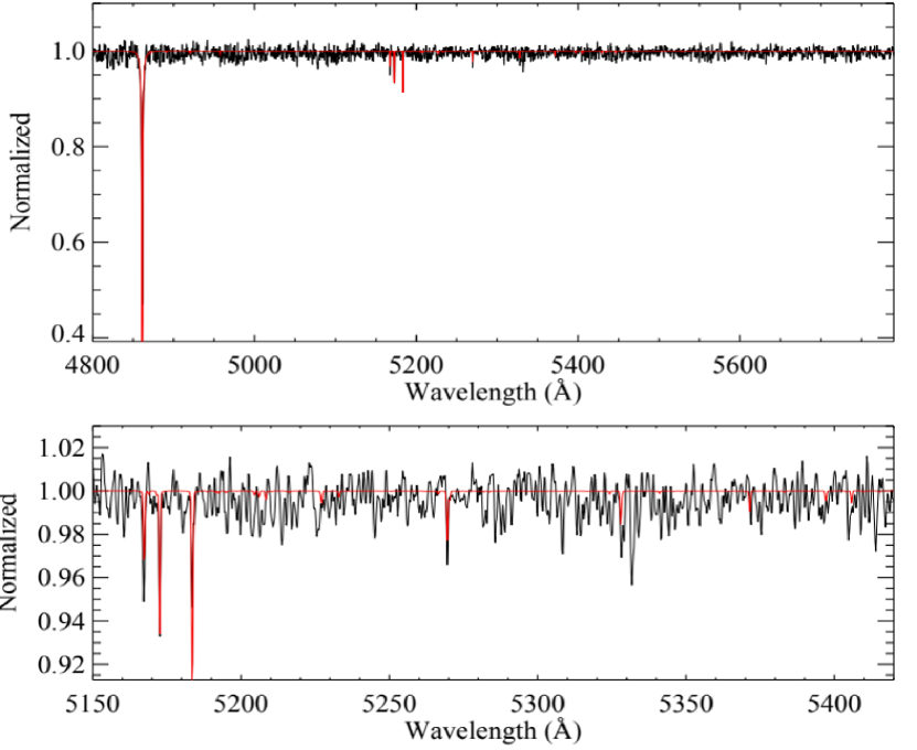
Figure 1: An example (J0226, one of the reference stars) of our spectral-matching technique. The black line is the observed spectrum, whereas the red is the best-matching synthetic spectrum. The bottom panel is a close-up view of the Mg I$b$ triplet region and a few iron lines.

3.2 Measurement of Equivalent Widths

To determine accurate stellar parameters and abundances of various chemical elements, we need to measure the equivalent widths (EWs) of Fe lines, as well as other metallic lines that are detectable in a spectrum. For this, we collected the information for various atomic lines from several literature sources (Aoki et al., 2013, 2018; Spite et al., 2018; Placco et al., 2020; Rasmussen et al., 2020). Then, the EWs were measured via fitting a Gaussian profile, using the Image Reduction and Analysis Facility (IRAF; Tody, 1986, 1993) task splot. We did not measure EWs for blended lines, but only for well-isolated lines. The line information of Li, C, and Ba were produced with the linemake code (Placco et al., 2021), and their abundances were determined through spectral synthesis rather than the EW analysis. Table 6 in the Appendix lists the line information used for the abundance analysis.

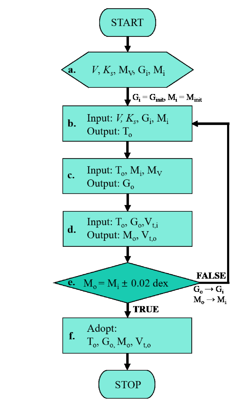
Figure 2: Flow chart of our iterative procedure to determine $T_{\rm eff}$, $\log~{}g$, [Fe/H], and $\xi_{\rm t}$. For convenience, the effective temperature, surface gravity, metallicity, and microturbulence velocity are expressed as T, G, M, and V_t, respectively. $M_{\rm V}$ is the absolute $V$ magnitude.

3.3 An Iterative Procedure for Determining Stellar Parameters

Because our targets are low-metallicity stars with weak metallic absorption lines, and the GRACES spectra have relatively lower S/N in the wavelength region shorter than 4700 Å, which includes many iron lines that play a crucial role in constraining the stellar parameters, we did not follow the traditional ionization-equilibrium technique to derive $T_{\rm eff}$, $\log~{}g$, and $\xi_{\rm t}$. Instead, we have devised an iterative procedure to determine the stellar parameters, as illustrated in Figure 2. It begins with the information on $V$, $K_{\rm s}$, $M_{\rm V}$, and the initial stellar parameters obtained by the spectral-matching procedure described above. Note that for brevity we express effective temperature as T, surface gravity as G, metallicity as M, and microturbulence velocity ($\xi_{\rm t}$) as V_t. A detailed description of the procedure is as follows:

Step a

Preparation of required information. We gather information on $V$, $K_{\rm s}$, $M_{\rm V}$, G_init, and M_init of each star, where $M_{\rm V}$ is the absolute $V$ magnitude, and G_init and M_init are the gravity and the metallicity, respectively, estimated from the spectral matching. The adopted $V$, $K_{\rm s}$, and M_V for our program stars are listed in Table 2.

Step b

Estimation of effective temperature. We input $V$, $K_{\rm s}$, G_i (G_init), and M_i (M_init), and estimate three $T_{\rm eff}$ values for each star by following the procedure described in Section 3.3.1. The gravity G_i is used to separate giants from dwarfs. We obtain a bi-weight average $T_{\rm eff}$ (T_o) from the three estimates.

Step c

Estimation of surface gravity. Following the prescription in Section 3.3.2, we estimate $\log~{}g$ (G_o), based on isochrone fitting. We assume a stellar age of 13 Gyr and [$\alpha$/Fe] = +0.3, appropriate for our EMP candidates. In this step, the inputs are T_o, M_i, and $M_{\rm V}$.

Step d

Estimation of metallicity and microturbulence velocity. While fixing T_o and G_o determined in Step b and Step c, we estimate M_o and V_t,o by the prescription addressed in Section 3.3.3.

Step e

Convergence check. We check if M_i and M_o agree with each other within $\pm$0.02 dex. If the convergence criterion is satisfied, the routine goes to Step f, and if not, it goes back to Step b, and G_o and M_o are used as G_i and M_i to repeat until it converges to the tolerance level of 0.02 dex in the metallicity difference between the input and output.

Step f

Determination of adopted stellar parameters. If the convergence criterion is met in Step e, the derived T_o, G_o, M_o, and V_t,o are taken as the adopted stellar parameters.

3.3.1 Effective Temperature

We employed three different methods to derive accurate and precise effective temperature estimates. The underlying principle of the methods is the InfraRed Flux Method (IRFM) method, which is based on the extinction-corrected $V-K_{\rm s}$ color-$T_{\rm eff}$ relation. We adopted the color-temperature relations provided by Alonso et al. (1999), González Hernández & Bonifacio (2009), and Casagrande et al. (2010). These studies reported different relations over a range of the surface gravities of stars, and by following their prescription, we made use of Equations 8 and 9 in Table 2 of Alonso et al. (1999) for giants, Equation 10 of González Hernández & Bonifacio (2009) for giants and dwarfs, and Equation 3 of Casagrande et al. (2010) for subgiants and dwarfs. All of these equations have some dependency on the metallicity, with valid ranges of [Fe/H] and $V-K_{\rm s}$.

We require $V-K_{\rm s}$, $\log~{}g$, and [Fe/H] information to work with the above equations. The criteria for subdividing the luminosity class of a star are $\log~{}g$ $\leq$ 3.0 for a giant, 3.0 $<$ $\log~{}g$ $\leq$ 3.75 for a subgiant, and $\log~{}g$ $>$ 3.75 for a dwarf. As Equations 8 and 9 of Alonso et al. (1999) use the same color range for a giant, we derived the temperature from both equations and took an average. If the $V-K_{\rm s}$ color is out of the range specified in a color-temperature relation, the effective temperature was determined by using the color range closest to the observed one. Through this process, we obtained two estimates of $T_{\rm eff}$ for each object.

In addition, we introduced the method by Frebel et al. (2013) to correct the spectroscopically determined $T_{\rm eff}$ from the spectral fitting. They reported a procedure of adjusting the systematic offset between the photometric and spectroscopic based $T_{\rm eff}$. This provides a third $T_{\rm eff}$ estimate. We ultimately calculated a bi-weight $T_{\rm eff}$ estimate from the three $T_{\rm eff}$ determinations for each star. We then follow the iterative process laid out in Figure 2 until convergence occurs, and a final adopted $T_{\rm eff}$ is obtained. Note that for the first trial of the $T_{\rm eff}$ estimate from the color-temperature relations, we adopted $\log~{}g$ and [Fe/H] derived by the spectral-fitting method. We used the final adopted $T_{\rm eff}$ for the abundance analysis. The standard error of the three temperatures is reported as the uncertainty in $T_{\rm eff}$ of each star.

Table 3: Determined Atmospheric Parameters

Short	$T_{\rm eff}$	$\log~{}g$	[Fe/H]	$\xi_{\rm t}$
ID	(K)			(km s-1)
J0010	4309$\pm$81	$0.34~{}^{+0.23}_{-0.26}$	–2.48$\pm$0.11	2.3
J0102	5974$\pm$35	$4.55~{}^{+0.02}_{-0.02}$	–3.09$\pm$0.06	0.7
J0158	5165$\pm$44	$2.48~{}^{+0.15}_{-0.14}$	–3.04$\pm$0.05	1.7
J0226	5461$\pm$98	$3.00~{}^{+0.29}_{-0.23}$	–3.78$\pm$0.05	1.9
J0357	5631$\pm$27	$3.49~{}^{+0.00}_{-0.04}$	–2.75$\pm$0.05	1.2
J0422	5027$\pm$48	$2.07~{}^{+0.17}_{-0.15}$	–3.33$\pm$0.06	2.3
J0713	4380$\pm$91	$0.22~{}^{+0.19}_{-0.20}$	–3.15$\pm$0.08	2.3
J0758	6453$\pm$254	$4.33~{}^{+0.14}_{-0.20}$	–2.96$\pm$0.13	1.0
J0814	5853$\pm$237	$3.52~{}^{+0.16}_{-0.22}$	–3.39$\pm$0.05	1.2
J0908	4713$\pm$145	$1.21~{}^{+0.40}_{-0.32}$	–3.67$\pm$0.06	2.3
J0925	5631$\pm$111	$3.39~{}^{+0.09}_{-0.14}$	–3.53$\pm$0.06	1.8
J1037	6569$\pm$423	$4.37~{}^{+0.16}_{-0.28}$	–2.50$\pm$0.05	1.3
J1311	6510$\pm$237	$4.23~{}^{+0.19}_{-0.30}$	–2.74$\pm$0.04	1.0
J1317	6810$\pm$336	$4.25~{}^{+0.11}_{-0.17}$	–2.37$\pm$0.05	1.3
J1522	5698$\pm$27	$3.43~{}^{+0.01}_{-0.04}$	–3.70$\pm$0.06	1.5
J1650	6800$\pm$335	$3.95~{}^{+0.02}_{-0.05}$	–2.17$\pm$0.05	1.3
J1705	6580$\pm$238	$4.29~{}^{+0.12}_{-0.16}$	–2.64$\pm$0.05	1.3
J2241	6608$\pm$152	$3.94~{}^{+0.05}_{-0.02}$	–2.71$\pm$0.13	0.7
J2242	4857$\pm$144	$1.46~{}^{+0.52}_{-0.39}$	–3.40$\pm$0.08	2.3
J2341	4628$\pm$46	$0.96~{}^{+0.17}_{-0.15}$	–3.17$\pm$0.07	2.3

Note. — The objects named J0226 and J1522 are the reference stars studied by Ito et al. (2013) and Matsuno et al. (2017), respectively.

3.3.2 Surface Gravity

Iron abundances estimated from Fe I lines are known to suffer from large non-local thermodynamic equilibrium (NLTE) effects (e.g., Lind et al., 2012; Amarsi et al., 2016), and the number of available Fe II lines is very limited in the GRACES spectra for our EMP candidates. This makes it difficult to determine the surface gravity by the traditional approach of the ionization equilibrium (forcing a balance between abundances estimated from the neutral atomic lines and singly ionized lines).

Instead, we determine the surface-gravity estimate through fitting isochrones. For this technique to work, we first generated a hundred isochrones with metallicities resampled from a normal distribution with an estimated [Fe/H] and a conservative error of 0.2 dex. In this process, we employed Yonsei-Yale ($Y^{2}$; Kim et al., 2002; Demarque et al., 2004) isochrone, and assumed a stellar age of 13 Gyr and [$\alpha$/Fe] = +0.3. Since the minimum value of [Fe/H] is –3.75 in the $Y^{2}$ isochrone, any metallicity of our target lower than this limit was forced to be [Fe/H] = –3.75.

In the $M_{\rm V}$-$T_{\rm eff}$ plane based on the generated isochrones, we searched for a gravity that most closely reflected the observables ($M_{\rm V}$ and $T_{\rm eff}$) of our target. We took a median value from one hundred such gravity estimates. The errors were taken at 34% to the left and right from the median in the $\log~{}g$ distribution. When the metallicity tolerance is satisfied, as illustrated in Figure 2, the final estimate of $\log~{}g$ is adopted.

3.3.3 Metallicity and Microturbulence Velocity

The metallicity was determined by minimizing the slope of log(EWs) of Fe I lines as a function of excitation potential. In this process, a total of 129 Fe I lines were used, and a starting model atmosphere was generated with $T_{\rm eff}$, $\log~{}g$, and [Fe/H] estimated in Step b, Step c, and the spectral fitting, respectively. The $\xi_{\rm t}$ value was assumed according to the evolutionary stage ($\xi_{\rm t}$ = 0.5 km s^-1 for dwarfs, 1.0 km s^-1 for turnoff stars, and 2.0 km s^-1 for giants). We adopted Kurucz model atmospheres (Castelli & Kurucz, 2003), using newly calculated opacity distribution functions with updated opacities and abundances (Castelli & Kurucz, 2004). A desired model atmosphere was created by interpolating the existing grid at given stellar parameters, using the ATLAS9 code (Castelli et al., 1997).

Note that, because Fe II lines are less subject to NLTE effects (e.g., Lind et al., 2012; Amarsi et al., 2016), it is desirable to use their abundance. However, because detectable Fe II lines are very limited for our EMP targets, we used the abundance derived from the Fe I lines. The uncertainty of [Fe/H] is given by the standard error of mean of the Fe I abundances.

The microturbulence velocity ($\xi_{\rm t}$) of a star was estimated by seeking a flat slope of log (EWs) for Fe I lines as a function of the reduced equivalent width, log (EWs/$\lambda$). We used the line-analysis program MOOG (Sneden 1973; Sobeck et al. 2011). As shown in Figure 2, if the metallicity M_o agrees with M_i within a difference of $\pm$0.02 dex, then T_o, G_o, M_o, and V_t,o are adopted as the final stellar parameters. When the absolute difference between M_i and M_o is larger than 0.02 dex, M_i is updated by M_o, and the routine run again until the metallicity tolerance is satisfied. Note that we do not update the $\xi_{\rm t}$ value when repeating the routine.

Table 3 lists the derived stellar parameters by the iterative procedure. According to the table, we have confirmed 8 VMP and 10 EMP stars, except two objects (J0226 and J1522), which were already analyzed by Ito et al. (2013) and Matsuno et al. (2017), respectively. We observed these objects as benchmark stars, and re-analyzed them to validate our approach to determining the stellar parameters and chemical abundances. In Section 4.4, we present a detailed comparison between our estimates and those of the previous studies.

Figure 3 shows the position of our program stars in the $\log~{}g$-$T_{\rm eff}$ plane, together with isochrones with age 13 Gyr and [$\alpha$/Fe] = +0.3, for [Fe/H] = –2.5, –3.0, and –3.5, represented by blue-dotted, orange-dashed, and green-solid lines, respectively. The turnoff stars are indicated with squares, while the giants are indicated circles. The dwarfs and subgiants are denoted by triangles. The two benchmark stars are represented by diamonds (black for J0226 and red for J1522). It is clear to see that our program stars populate a wide range of luminosity classes and spectral types.

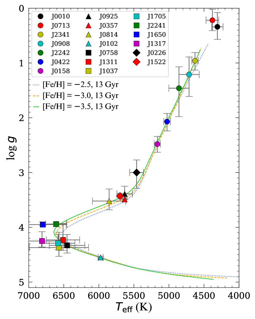
Figure 3: Adopted surface gravity, as a function of effective temperature, for our program stars. They are grouped into three different symbols according to $T_{\rm eff}$. The square symbols represent turnoff stars, while the circle symbols represent cool giants. The dwarfs and subgiants are denoted by triangles. The two comparison stars are symbolized by diamonds (black for J0226 and red for J1522). The three isochrones shown, with age 13 Gyr and [$\alpha$/Fe] = +0.3, represent [Fe/H] = –2.5 (blue dotted), [Fe/H] = –3.0 (orange dashed), and [Fe/H] = –3.5 (green solid).

4 Elemental Abundances

To derive the abundances of individual elements, we carried out a one-dimensional (1D), local thermodynamic equilibrium (LTE) abundance analysis and spectral synthesis using MOOG. We adopted the solar atmospheric abundances in Asplund et al. (2009) to determine the abundance ratios relative to the Sun. Whenever difficulties in measuring the EWs of a line arose, we also performed spectral synthesis. The atomic line data were compiled from several literature sources (Aoki et al., 2013, 2018; Spite et al., 2018; Placco et al., 2020; Rasmussen et al., 2020); and the line information is listed in Table 6 in the Appendix. In this section, we address how we derived the chemical abundances.

4.1 Chemical Abundances by Equivalent Width Analysis

We derived the abundances for the odd-$Z$ elements (Na, K, and Sc), $\alpha$-elements (Mg and Ca), and iron-peak elements (Cr, Mn, Ni, and Zn) by measuring the EWs of their neutral or singly ionized lines. The Na abundance was determined using the Na I doublet located at 5889 Å and 5895 Å, which are the only available sodium lines in low-metallicity stars.

Only one line at 7699 Å was used to measure the K abundance, while five Sc II lines were used to measure [Sc/Fe]. We used four Mg I and 12 Ca I lines to derive Mg and Ca abundance ratios, respectively.

Concerning the abundances of the iron-peak elements, we utilized 10 Cr I, 3 Mn I, 15 Ni I, and 2 Zn I lines to determine [Cr/Fe], [Mn/Fe], [Ni/Fe], and [Zn/Fe], respectively. Depending on the effective temperature, metallicity, and S/N of a spectrum, the number of measured EWs for each element differs from star to star.

4.2 Chemical Abundances by Spectral Synthesis

The abundance ratios for Li, C, and Ba were determined by spectral synthesis, using atomic line data from linemake. For the Li abundance ratio, we used the Li I resonance doublet line around 6707 Å. Figure 4 provides an example of the Li spectral synthesis (J0357). The black-solid line is the observed spectrum; the red-dashed line is the best-matching synthetic spectrum. The two dotted lines present the upper and lower limits of the spectral fits by deviating by $\pm$0.2 dex in $A$(Li) from the best-matching one. We conservatively considered these limits as the error of the determined [Li/Fe].

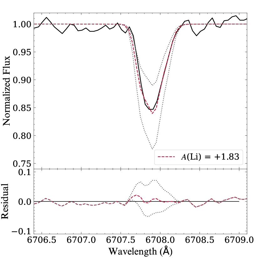
Figure 4: Top panel: Example of Li spectral synthesis for one of our program stars (J0357). The black-solid line is the observed spectrum, and the red-dashed line is the best-matching synthetic spectrum. The two dotted lines are the upper and lower limits of the spectral fits, which deviate by $\pm$0.2 dex. Bottom panel: Residual plot of the top panel.

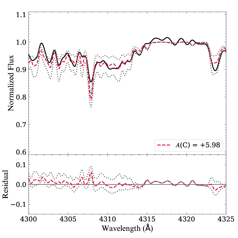
Figure 5: Same as in Figure 4, but for C and J0226.

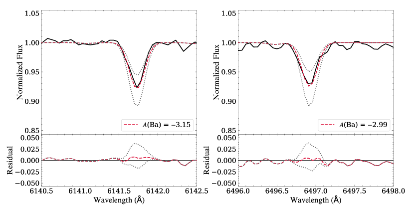
Figure 6: Same as in Figure 4, but for Ba and J0713.

Table 4: [X/Fe] Abundance Ratios for Program Stars

ID	Li I	C	Na I	Mg I	K I	Ca I	Sc II	Cr I	Mn I	Ni I	Zn I	Ba II
J0010	$\cdots$	0.37	0.24$\pm$0.07	0.73$\pm$0.04	0.13$\pm$0.09	0.19$\pm$0.05	–0.33$\pm$0.11	–0.10$\pm$0.05	0.09$\pm$0.06	0.13$\pm$0.05	0.00$\pm$0.12	–1.72$\pm$0.06
J0102	3.79	0.75	–0.60$\pm$0.12	0.21$\pm$0.12	$\cdots$	$\cdots$	$\cdots$	–0.04$\pm$0.17	$\cdots$	$\cdots$	$\cdots$	$\cdots$
J0158	2.78	0.11	1.14$\pm$0.08	0.06$\pm$0.06	$\cdots$	0.41$\pm$0.04	$\cdots$	–0.09$\pm$0.06	–0.01$\pm$0.10	0.30$\pm$0.06	0.61$\pm$0.10	$<$–1.60$\pm$0.20
J0226	$\cdots$	1.33	0.29$\pm$0.04	0.59$\pm$0.05	$\cdots$	$\cdots$	$\cdots$	$\cdots$	$\cdots$	$\cdots$	$\cdots$	$\cdots$
J0357	3.53	0.40	0.13$\pm$0.07	0.34$\pm$0.04	$\cdots$	0.33$\pm$0.03	0.50$\pm$0.10	–0.16$\pm$0.05	0.01$\pm$0.09	0.37$\pm$0.07	0.81$\pm$0.10	–0.70$\pm$0.04
J0422	$\cdots$	$<$0.11	–0.46$\pm$0.08	0.18$\pm$0.04	$\cdots$	0.21$\pm$0.05	$\cdots$	–0.36$\pm$0.08	$\cdots$	0.23$\pm$0.08	$\cdots$	–1.15$\pm$0.20
J0713	$\cdots$	0.08	0.37$\pm$0.08	0.31$\pm$0.06	0.18$\pm$0.10	0.00$\pm$0.05	–0.26$\pm$0.10	–0.33$\pm$0.03	–0.02$\pm$0.10	–0.01$\pm$0.04	0.31$\pm$0.13	–2.08$\pm$0.04
J0758	$\cdots$	$<$1.20	–0.75$\pm$0.24	0.06$\pm$0.17	$\cdots$	$\cdots$	$\cdots$	–0.11$\pm$0.24	$\cdots$	$\cdots$	$\cdots$	$\cdots$
J0814	4.10	$<$1.10	–0.05$\pm$0.05	0.33$\pm$0.04	$\cdots$	0.61$\pm$0.07	$\cdots$	$\cdots$	$\cdots$	$\cdots$	$\cdots$	$\cdots$
J0908	$\cdots$	$<$0.01	–0.19$\pm$0.08	0.17$\pm$0.07	0.96$\pm$0.11	0.35$\pm$0.04	$\cdots$	–0.47$\pm$0.08	$\cdots$	0.35$\pm$0.08	$\cdots$	$<$–1.40$\pm$0.20
J0925	3.80	1.40	–0.28$\pm$0.05	0.35$\pm$0.05	$\cdots$	$\cdots$	$\cdots$	$\cdots$	$\cdots$	$\cdots$	$\cdots$	$\cdots$
J1037	3.66	1.10	–0.41$\pm$0.06	0.30$\pm$0.03	$\cdots$	0.12$\pm$0.03	$\cdots$	–0.24$\pm$0.09	$\cdots$	0.34$\pm$0.09	$\cdots$	$\cdots$
J1311	$\cdots$	$<$1.10	–0.12$\pm$0.03	–0.22$\pm$0.03	$\cdots$	$\cdots$	$\cdots$	–0.35$\pm$0.02	$\cdots$	$\cdots$	$\cdots$	$<$–0.20$\pm$0.20
J1317	3.73	$<$0.60	–0.08$\pm$0.08	0.30$\pm$0.06	$\cdots$	0.24$\pm$0.05	$\cdots$	–0.09$\pm$0.11	$\cdots$	0.69$\pm$0.06	$\cdots$	$\cdots$
J1522	4.30	$<$1.03	$\cdots$	0.42$\pm$0.07	$\cdots$	$\cdots$	$\cdots$	$\cdots$	$\cdots$	$\cdots$	$\cdots$	$\cdots$
J1650	3.47	$<$0.30	–0.60$\pm$0.10	0.13$\pm$0.07	0.69$\pm$0.14	0.35$\pm$0.04	$\cdots$	–0.22$\pm$0.10	$\cdots$	0.73$\pm$0.10	$\cdots$	$<$–0.64$\pm$0.20
J1705	3.55	$<$0.30	–0.44$\pm$0.06	0.25$\pm$0.03	$\cdots$	0.30$\pm$0.02	$\cdots$	–0.07$\pm$0.08	$\cdots$	$\cdots$	$\cdots$	$<$–0.50$\pm$0.20
J2241	$\cdots$	$<$1.30	–0.60$\pm$0.15	–0.61$\pm$0.15	$\cdots$	$\cdots$	$\cdots$	$\cdots$	$\cdots$	$\cdots$	$\cdots$	$<$–0.50$\pm$0.20
J2242	$\cdots$	0.05	–1.02$\pm$0.26	0.24$\pm$0.04	1.48$\pm$0.36	0.71$\pm$0.14	–0.11$\pm$0.36	0.01$\pm$0.26	$\cdots$	0.89$\pm$0.36	$\cdots$	$\cdots$
J2341	$\cdots$	0.03	0.74$\pm$0.10	0.36$\pm$0.04	0.59$\pm$0.12	0.25$\pm$0.04	0.09$\pm$0.07	–0.38$\pm$0.04	$\cdots$	0.07$\pm$0.09	$\cdots$	–1.61$\pm$0.06

Note. — The errors of Li and C are conservatively assumed to be 0.2 dex; see text for the errors estimated for other elements. The $<$ symbol indicates the upper limit estimate. Note that the [C/Fe] value is corrected for the evolutionary stage following the prescription of Placco et al. (2014). The applied correction is listed in Table 7 in the Appendix.

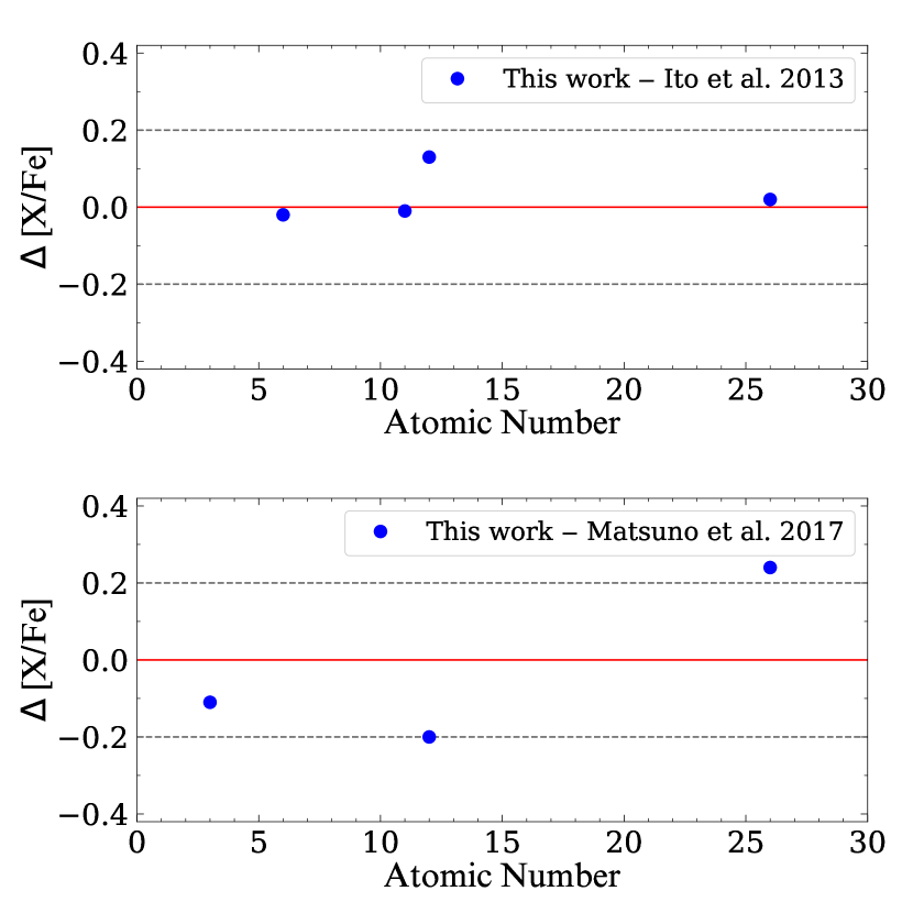
Figure 7: Differences in the chemical abundances between our study and the work by Ito et al. (2013) (top panel) and Matsuno et al. (2017) (bottom panel). The red-solid line shows the zero point, while the gray-dashed lines indicate deviations of $\pm$0.2 dex.

We estimated the C-abundance ratio by spectral synthesis of the CH $G$-band around 4310 Å. While estimating [C/Fe], we adopted ¹²C/¹³C of 89 ($\log~{}g$$>$ 3.75), 30 (3.0 $<$ $\log~{}g$ $\leq$ 3.75), or 20 ($\log~{}g$ $\leq$ 3.0) according to the luminosity class of our program stars (Asplund et al., 2009), and we used spectra degraded to $R$ = 10,000 in order to increase the S/N around this feature. Figure 5 exhibits an example of the spectral synthesis for the carbon-abundance determination (J0226). As before, the observed spectrum is represented by the black line, while the best-matching synthetic spectrum is represented by the red-dashed line. The upper and lower limits of the spectral fits are denoted by the two dotted lines, which are located at $\pm$0.2 dex away from the determined value. This limit is considered as the uncertainty of the estimated [C/Fe]. We corrected the determined [C/Fe] following the prescription of Placco et al. (2014) to restore the natal carbon on the surface of stars that have been altered due to evolutionary effects (the depletion of C as stars climb the giant branch). Table 7 in the Appendix summarizes the measured [C/Fe] and its corrected value for each object.

We were able to measure the abundance of one of the neutron-capture elements (Ba), using two Ba II lines at 6141 Å and 6497 Å, through spectral synthesis. Isotopic splitting using the values from Sneden et al. (2008) and hyperfine structure were considered when the line information is generated with linemake. An example is displayed in Figure 6; the lines are the same as in Figure 4. The error estimate comes from the standard error of the two estimates, or is conservatively set to 0.2 dex for the objects with only one line available.

4.3 Errors of Derived Abundances

When computing the error in the derived abundance for individual elements, we have considered both the random errors arising from the line-to-line scatter and the systematic error caused by the errors of the adopted stellar parameters. The random error represents the variation of the individual lines for a given element, calculated by $\sigma/\sqrt{N}$, where $N$ is the number of lines and $\sigma$ is the standard deviation of the derived abundance. This has the advantage of including the uncertainty from the oscillator strength values of the lines considered. In case for an element where the number of detectable lines is less than three, we took $\sigma$ from the Fe I lines and computed its standard error by $\sigma$(Fe I)/$\sqrt{N}$.

To derive the systematic error due to stellar atmospheric-parameter errors, we perturbed the stellar parameters by $\pm$100 K for $T_{\rm eff}$, $\pm$0.2 dex for $\log~{}g$, and $\pm$0.2 km s^-1 for $\xi_{\rm t}$ one at a time, and estimated the systematic error for each case. The systematic error for each parameter is an average of the two values derived by perturbing two ways ($\pm$). The final reported error on the abundance of each element is the quadratic sum of the random error and the systematic error. Table 4 summarizes the estimated abundances for our program stars; Table 8 in the Appendix provides more detailed abundances and their associated errors measured for our VMP stars.

4.4 Abundance Comparison with Previous Studies

Among our sample of stars, two objects (J0226 and J1522) were previously studied by Ito et al. (2013) and Matsuno et al. (2017), respectively. The two studies observed these stars with Subaru/HDS to obtain high-resolution ($R\sim$ 60,000) spectra, and carried out a detailed abundance analysis. We observed these stars to validate the strategy of our stellar parameter and abundance determination by comparing our estimates with their values.

We intentionally observed the bright ($V\sim$ 9.1) object J0226 multiple times with different exposure times to obtain spectra with a range of S/N. This provides an opportunity to check how the S/N of a spectrum affects the derivation of the stellar parameters and abundances. By comparing the literature stellar parameters and chemical abundances with the ones derived from our spectrum that has similar S/N to the rest of our program stars, we can appreciate if the stellar parameters and abundances are reliable at S/N ($\sim$ 60), which is the mean S/N of the relatively bright ($g\leq$ 15.9) objects among our program stars. Similarly, the relatively faint object J1522 can be used to validate the derived abundance for the faint ($g>$ 15.9) objects with S/N $\sim$ 40.

We obtained $T_{\rm eff}$ = 5461 K, $\log~{}g$ = 3.0, [Fe/H] = –3.78 for the object J0226 from a GRACES spectrum with S/N = 75. Comparison with the stellar parameters estimated by Ito et al. (2013) reveals that our estimates are 30 K higher in $T_{\rm eff}$, 0.4 dex lower in $\log~{}g$, and 0.01 dex higher in [Fe/H], indicating good agreement. In addition, we compared the elemental differences in common between their study and our work, as shown in the top panel of Figure 7. The gray-dashed lines indicate the abundance deviation of $\pm$0.2 dex. The plot clearly indicates a good match within $\pm$0.2 dex, validating our abundance analysis.

The stellar parameters derived from our GRACES spectrum for J1522 are $T_{\rm eff}$ = 5698 K, $\log~{}g$ = 3.43, and [Fe/H] = –3.7. This object is relatively faint, and has a low S/N of 38. Comparing with the values reported by Matsuno et al. (2017), our estimates are about 200 K higher for $T_{\rm eff}$, 0.3 dex lower for $\log~{}g$, and 0.25 dex more metal-rich. We ascribe the [Fe/H] difference primarily to the temperature difference. We note that they adopted $T_{\rm eff}$ = 5505 K determined by fitting the H$\beta$ profile for their abundance analysis, instead of $T_{\rm eff}$ derived from $V-K_{\rm s}$, which is 5813 K, and much closer to our estimate. Nonetheless, in the bottom panel of Figure 7, we see that Li and Mg abundance agree within $\pm$0.2 dex, again validating our abundance determinations even at lower S/N. Note that in the figure, we did not include the carbon-abundance ratio because both theirs and ours are the upper limit estimate.

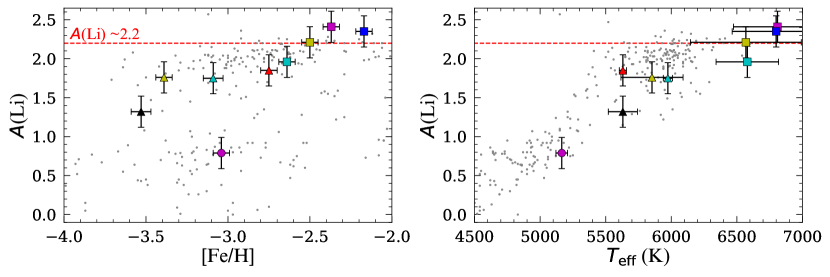
Figure 8: $A$(Li) distribution, as a function of [Fe/H] (left panel) and a function of $T_{\rm eff}$ (right panel). The colored symbols are our program stars, while the gray circles are gathered from Roederer et al. (2014). The red-dashed line indicates the Spite plateau at $A$(Li) = 2.2.

5 Discussion

In this section, we compare the chemical abundances of our program stars with those from other previously studied Galactic halo stars. We find that most of our program stars follow the general trends of the previous data for VMP stars. However, there are a few exceptional stars with peculiar abundances. We first discuss the overall abundance trends of individual elements, and then focus on the chemically peculiar objects. These stars will be valuable to provide constraints on rare astrophysical production sites or nucleosynthetic channels. Note that in the following discussion that we only consider 1D LTE abundances, to be consistent with other literature abundances, which are not generally corrected for either 3D or NLTE effects. We do not include the two benchmark stars in the following discussion.

5.1 Overall Abundance Trends

5.1.1 Lithium

Lithium is one of the most important elements, as its abundance can be used to constrain Big Bang nucleosynthesis. Figure 8 exhibits the behavior of the absolute Li abundances, $A$(Li), as a function of [Fe/H] (left panel) and $T_{\rm eff}$ (right panel). The colored symbols are our program stars, while the gray circles are adopted from Roederer et al. (2014), which are not corrected for NLTE effects. The stellar sequence located at $A$(Li) $\sim$ 2.2 for the region of –2.9 $<$ [Fe/H] is known as the Spite plateau (Spite & Spite, 1982). Although the location of the Spite plateau varies over $A$(Li) = 2.10 – 2.35 from study to study (e.g., Ryan et al., 1999, 2000; Bonifacio et al., 2010; Sbordone et al., 2010; Simpson et al., 2021), we indicate it as the red-dashed line at $A$(Li) = 2.2, which is the most commonly accepted value. The primordial Li predicted by the Big Bang nucleosynthesis is in the range $A$(Li) = 2.67 – 2.74 (Spergel et al., 2007; Cyburt et al., 2016; Coc & Vangioni, 2017); the difference between the primordial Li and the Spite plateau is known as the longstanding cosmological lithium problem.

Inspection of the figure reveals that our sample of stars follows the general trend of the other literature abundances, but there are some subtle differences as well. The object J0158 (magenta circle) with $A$(Li) $<$ 1.0 is a giant. When stars leave the main sequence (MS), their surface Li material is reduced by dilution caused by the first dredge-up (FDU). Observationally, we can see the difference in Li abundances between the turnoff (TO) stars and giants, and then the Li abundance for giants does not change much across a large range of [Fe/H] after the FDU to the red giant branch (RGB) bump (e.g., Lind et al., 2009). The Li abundance further decreases as a star ascends above the RGB bump ($\log~{}g$ $<$ 2.0), due to poorly understood extra mixing. This characteristic abundance pattern due to the stellar evolution is clearly seen in Figure 8.

Among our program stars, the four stars hotter than 6500 K have $A$(Li) values closely scattered around the Spite plateau, as can be seen in the right panel. These objects can be very useful to check the possibility of the extension of the Li plateau to the hotter temperature region, where relatively few data exist at present. Three stars (black, red, and yellow triangles) are subgiants, which are close to the giant phase (see Figure 3). Their Li abundance is slightly lower than the overall trend, probably due to the increasing convection zone. The object J0102 (cyan triangle) is a warm dwarf with [Fe/H] $<$ –3.0. Its expected convective zone is not very deep; hence its surface Li should be preserved without much destruction since its birth. However, its $A$(Li) is slightly lower than the Spite plateau. One possible cause of its lower $A$(Li) compared to the Spite plateau and other literature sample is the temperature scale we have adopted. It is known that a temperature difference of 100 K results in the change of 0.08 dex of $A$(Li). Consequently, it may be possible that our temperature scale is slightly lower for dwarf stars than the ones used in the literature. An analysis of a larger number of stars in a uniform and consistent manner is clearly critical when discussing the observed Li trend. A follow-up study of our TO and dwarf stars can provide useful constraints on the primordial lithium problem, considering their evolutionary stage and metallicity.

One more interesting aspect is that our sample of stars also gives a clue to a behavior known as the “double sequence” in the Spite plateau noted by Meléndez et al. (2010), whereby the stars with [Fe/H] $<$ –2.5 possess slightly lower $A$(Li) than the ones with [Fe/H] $>$ –2.5. The similar behavior was reported in other studies (e.g., Ryan et al., 1999, 2000; Sbordone et al., 2010), and we notice this characteristic in the figure as well.

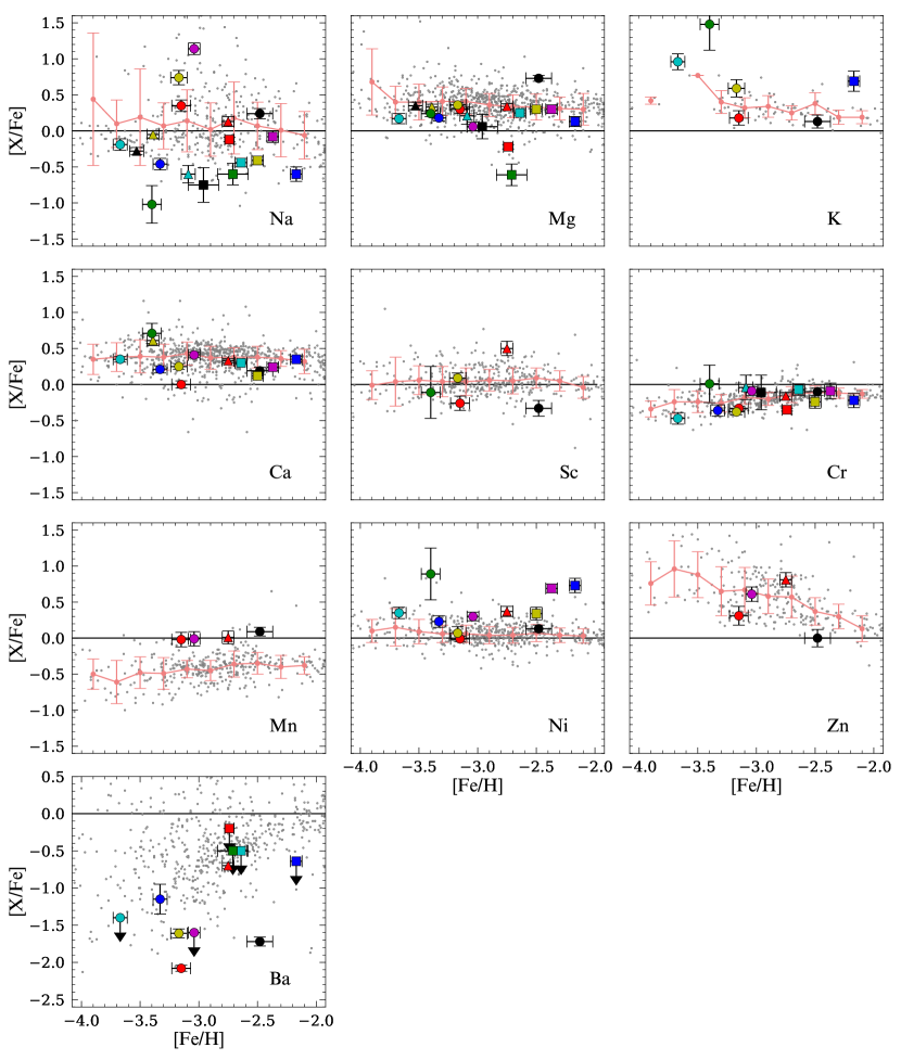
Figure 9: [X/Fe], as a function of [Fe/H], for the odd-$Z$ (Na, K, and Sc), $\alpha$- (Mg and Ca), iron-peak (Cr, Mn, Ni, and Zn), and neutron-capture (Ba) elements. Our program stars are represented by colored symbols, while the objects compiled from various literature sources (Venn et al., 2004; Aoki et al., 2013; Yong et al., 2013; Roederer et al., 2014) are shown with gray circles. The pink-solid line and error bars represent the 3$\sigma$-clipped mean trend and standard deviation of the literature sample for a bin size of 0.2 dex in [Fe/H], respectively. Our estimates are not included in these calculations. The black-dashed line denotes the solar abundance ratio. The colors and symbols for our program stars are the same as in Figure 3. The down arrow indicates an upper limit.

5.1.2 Odd-$Z$ Elements: Na, K, and Sc

Figure 9 compares our derived abundances with other previously studied Galactic VMP stars for the odd-$Z$ (Na, K, and Sc), $\alpha$- (Mg and Ca), iron-peak (Cr, Mn, Ni, and Zn), and neutron-capture (Ba) elements. Our program stars are represented by the large colored symbols, while the objects compiled from various literature sources are indicated by gray circles (Venn et al., 2004; Aoki et al., 2013; Yong et al., 2013; Roederer et al., 2014). Note that, even though the NLTE corrected values for some elements are available in some studies, we used LTE values for this comparison. The colors and symbols for our program stars are the same as in Figure 3. The pink-solid line and error bar represent the $3\sigma$-clipped mean trend and standard deviation for the literature sample using a bin size of 0.2 dex in [Fe/H], respectively. Our estimates are not included in the calculations. The black-solid line denotes the solar abundance ratio. Some selection biases may be underlying in the individual samples from the literature, according to their science goals. Nevertheless, Figure 9 can convey useful information on understanding the early chemical evolution of the MW, as well as for identifying the chemically peculiar objects.

Among the odd-$Z$ elements, we were able to derive Na, K, and Sc abundance ratios. The Na-abundance ratios of our program stars in Figure 9 show that many of them are consistently lower than the main trend (the pink line), even though some of them are in the range of other VMP stars. Sodium is formed during C-burning in massive stars, as well as during the hydrogen burning via the Ne-Na cycle (e.g., Romano et al., 2010). It is dispersed into the interstellar medium (ISM) by CCSNe as well as by mass loss from asymptotic giant branch (AGB) stars. Hence, the objects with [Na/Fe] $<$ –0.5 may be formed in isolated gas clouds, which were not well-mixed or chemically enriched by a few CCSNe or AGB stars. Two objects stand out in the figure (J0158 and J2242), with [Na/Fe] $>$ +1.0 and [Na/Fe] $<$ –1.0, respectively. We discuss these objects in more detail in Section 5.3.1.

Unlike Na, K and Sc are the product of explosive Si-burning and/or O-burning in the CCSN stage (Woosley & Weaver, 1995). They are also created by the $\nu$-process in CCSNe (Kobayashi et al., 2011). Hence, they are good probes for tracing the nucleosynthesis process in explosive events. We measured K abundances for six stars. Figure 9 indicates that the K-abundance trend increases with decreasing [Fe/H] for [Fe/H] $<$ –3.2; one of our program stars (J0908; cyan circle) is on this increasing trend. There are two objects (J1650 and J2242) at [Fe/H] $\sim$ –2.2 and –3.4, respectively, which possess much higher [K/Fe] than the other objects at the same metallicity, as further discussed in Section 5.3.1.

The Sc-abundance ratio was derived for five objects, and two of their abundances exhibit somewhat larger scatter than the other Galactic field stars, as can be seen in Figure 9. Studies (e.g., Chieffi & Limongi, 2002) show that its production depends on the mass of the CCSN progenitors. If stars have formed in gas clouds which were enriched by a few SNe from stars with different masses, we would expect to observe a large scatter in the Sc abundances, which may be the case for our program stars. It is known that Galactic chemical-evolution models do not reproduce the evolution of the observed K and Sc abundances; the model predictions are consistently lower than the observations for these two elements (e.g., Kobayashi et al., 2020).

5.1.3 Alpha Elements: Mg and Ca

The so-called $\alpha$-elements are mostly produced by the hydrostatic and explosive nucleosynthesis process in massive stars, and they are ejected into the interstellar space by CCSNe explosions. Specifically, Mg is produced through a hydrostatic nucleosynthetic process during the C-burning of a massive star. Calcium is mainly created during the O-burning of CCSNe. Although the $\alpha$-elements are mainly formed by CCSNe, some amount of Ca is also generated by SNe Ia (Iwamoto et al., 1999). Thus, the Mg abundance, which has a single production channel, is frequently used as an important tracer to examine the contribution of CCSNe. In addition, thanks to the strong Mg absorption lines, its abundance is readily measured from the spectra of VMP stars, and it has proven to be a powerful tool to track the star-formation history.

Among the $\alpha$-elements, we were able to derive the abundances of Mg for all our EMP candidates and Ca for 13 objects from the GRACES spectra. In Figure 9, we can observe that most of our targets exhibit a similar [Mg/Fe] trend at [Mg/Fe] $\sim$ +0.3, with small scatter relative to other VMP stars, but a few objects (J0010, J1311, and J2241) distinguish themselves from the rest. We discuss these objects in Section 5.3.2. The Ca abundance for most of our program stars exhibit a very small dispersion, following the trends of other VMP stars. The behavior of the observed $\alpha$-element abundances indicates that CCSNe had a dominant role in the chemical enrichment for our program stars.

5.1.4 Iron-peak Elements: Cr, Mn, Ni and Zn

Iron-peak elements are produced during Si-burning, and also can be synthesized in both SNe Ia and CCSNe (Kobayashi & Nomoto, 2009; Kobayashi et al., 2020). Since the innermost region of C+O white dwarfs is sufficiently hot to burn Si, iron-peak elements can also be synthesized (Hoyle & Fowler, 1960; Arnett et al., 1971) by this pathway. CCSNe contribute to explosive nucleosynthesis to form iron-peak elements in two distinct regions: incomplete and complete Si-burning regions (e.g., Hashimoto et al., 1989; Woosley & Weaver, 1995; Thielemann et al., 1996; Umeda & Nomoto, 2002). Chromium and Mn are synthesized in the incomplete Si-burning region in the ejecta of CCSNe, while Ni and Zn are produced in the complete Si-burning region of the deeper inner portion of the ejecta during the CCSN explosion.

We are able to determine the abundance of Cr, Mn, Ni, and Zn among the iron-peak elements for some of our program stars. Inspection of Figure 9 reveals that the overall trend of Cr, Mn, and Ni of the VMP/EMP stars exhibits a relatively small dispersion, but the Zn abundance shows a rather large scatter among the iron-group elements.

Similar to other Galactic VMP stars, the Cr abundances of our targets exhibit ordinary behavior, consistent with other literature results. The very small dispersion over a range of metallicities suggests that their formation is closely related (e.g., Reggiani et al., 2017). We also notice the declining trend with decreasing [Fe/H], suggesting chemical evolution driven by CCSNe in the early epochs of the MW.

Figure 9 indicates the most of the Galactic field stars exhibit a decreasing trend of the Mn abundance with decreasing metallicity, similar to the Cr abundance, supporting the claim of early chemical enrichment from CCSNe. We have measured the Mn abundance for four stars. It can be seen in Figure 9 that their abundances are near the solar value, independent of their metallicity, and appear elevated compared to the main locus. However, the absorption lines of Mn are often too weak in VMP/EMP stars, causing systematic uncertainty. This might be the case for our targets, and three of the four objects rely on one line, resulting in uncertain measurements. An abundance analysis based on higher-quality spectra are required to confirm the Mn enhancements in our four program stars.

The Ni abundances of the previously studied VMP stars are generally close to the solar level, as are some of our program stars. Notably, we observe three objects (J1317, J1650, and J2242) that have [Ni/Fe] $>$ +0.5. We further discuss the objects J1650 and J2242 in Section 5.3.1. The abundances for elements other than Ni in J1317 appear normal, so it may have been enriched by SNe Ia, considering its relatively high metallicity. However, the Ni abundance is derived from one absorption line, and its uncertainty is rather large; its chemical peculiarity is desirable to confirm with additional lines.

In Figure 9, the average Zn-abundance pattern tends to increase with decreasing metallicity. This trend has been argued to be caused by problems detecting the Zn lines at low metallicity (see Yong et al. 2021 for a more detailed discussion). This is particularly problematic for EMP stars. These factors may explain the larger dispersion of Zn compared to other iron-peak elements. Notwithstanding, the Zn-abundance trend can be used to understand the physics of CCSNe. Zinc is generated in the deepest region of hypernovae (HNe; Umeda & Nomoto, 2002), and a more significant explosion energy leads to higher [Zn/Fe] ratios (Nomoto et al., 2013). Consequently, HNe may be responsible for higher values of [Zn/Fe] at the lowest metallicity.

5.1.5 Neutron-capture Element: Ba

Heavier elements beyond the iron peak are created by capturing neutrons and their subsequent $\beta$-decay. At least two processes – the slow ($s$-) and rapid ($r$-) neutron-capture processes – are thought to be responsible for the synthesis of these elements. An intermediate neutron-caption process (the $i$-process; Cowan & Rose 1977) may also be involved. The slow neutron-capture process occurs in an environment where the neutron flux is much lower than the rapid neutron-capture process. The main $r$-process elements are created during violent events such as CCSNe, neutron star mergers, gamma ray burst, etc. (Nishmura et al., 2015; Drout et al., 2017; Côté et al., 2019; Siegel et al., 2019), whereas the main $s$-process elements are produced during the AGB phase of low-mass stars (Suda et al., 2004; Herwig, 2005; Komiya et al., 2007; Masseron et at., 2010; Lugaro et al., 2012). A number of sites have been suggested for the $i$-process, including AGB stars (Hampel et al., 2016; Cowan et al., 2021; Choplin et al., 2022) and rapidly accreting white dwarfs (Denissenkov et al., 2017, 2019; Côté et al., 2018).

In the GRACES spectra of our program stars, the only measurable lines for neutron-capture elements are two Ba II lines. We took an average of the abundances derived from these two lines. The bottom panel of Figure 9 displays [Ba/Fe] as a function of [Fe/H] for our sample (colored symbols) and other field stars. We clearly observe a very large scatter especially in the low-metallicity region, and all our program stars have [Ba/Fe] $<$ 0. The large spread of the Ba abundance at low metallicity is a well-known pattern (Ryan et al., 1996; Aoki et al., 2005; Roederer, 2013).

Because the favored astrophysical site for the operation of the $s$-process is AGB stars, stars with the lowest metallicity, and oldest ages, do not have sufficient time to be polluted by progenitors during their thermally pulsing AGB phase. Instead, in the early Universe, Ba could be produced by the $r$-process in massive stars (Travaglio et al., 1999; Cescutti et al., 2006), or by fast rotating, low-metallicity stars (Frischknecht et al., 2016; Choplin et al., 2018). Thus, we expect the Ba abundance for our EMP stars was probably produced by the main $r$-process. In both cases, the main neutron source is the ²²Ne($\alpha$,$n$)²⁵Mg reaction. In addition, due to inefficient mixing of the ISM in the early Galaxy, stars born in giant molecular clouds polluted by single SN may have unusually high Ba. However, we do not see evidence for this in our sample, as all our stars exhibit low Ba abundances ([Ba/Fe] $<$ 0.0).

Although we are not able to measure Sr abundances for our program stars, other studies (e.g., Spite et al., 2014; Cowan et al., 2021; Matas Pinto et al., 2021) reported a large scatter of [Sr/Ba] among the VMP stars, indicating that a Ba-poor star can still be Sr-rich. This leads to invoking other processes, such as a non-standard $s$-process (e.g., Frischknecht et al., 2016) and the $i$-process (Cowan & Rose, 1977; Hampel et al., 2016). These mechanisms are believed to be relatively dominant only in Ba-deficient stars. Additional follow-up studies to determine the Sr abundance ratio for our program stars will be valuable to confirm these characteristics.

Recently, Li et al. (2022) reported two different behaviors of Ba abundance ratios for their VMP giant sample. The stars with [Fe/H] $<$ –3.0 exhibit much lower [Ba/Fe] than the ones with [Fe/H] $>$ –3.0. Although we do not observe the pattern from our giants, the inclusion of the TO stars reveals a similar behavior. Furthermore, the plot for [Ba/Fe] indicates that most of stars with [Ba/Fe] $<$ –1.0 have [Fe/H] $<$ –3.0, and are giants. Li et al. (2022) also found such a feature in their sample. The variety of Ba abundances for VMP stars suggests stochastic pollution from neutron-capture elements in the chemical evolution of the early MW.

One intriguing object is J0713, which has the lowest [Ba/Fe] among our sample. Given that there is nothing unusual in other abundances, this object may be born in a natal cloud having no association with a neutron-capture event.

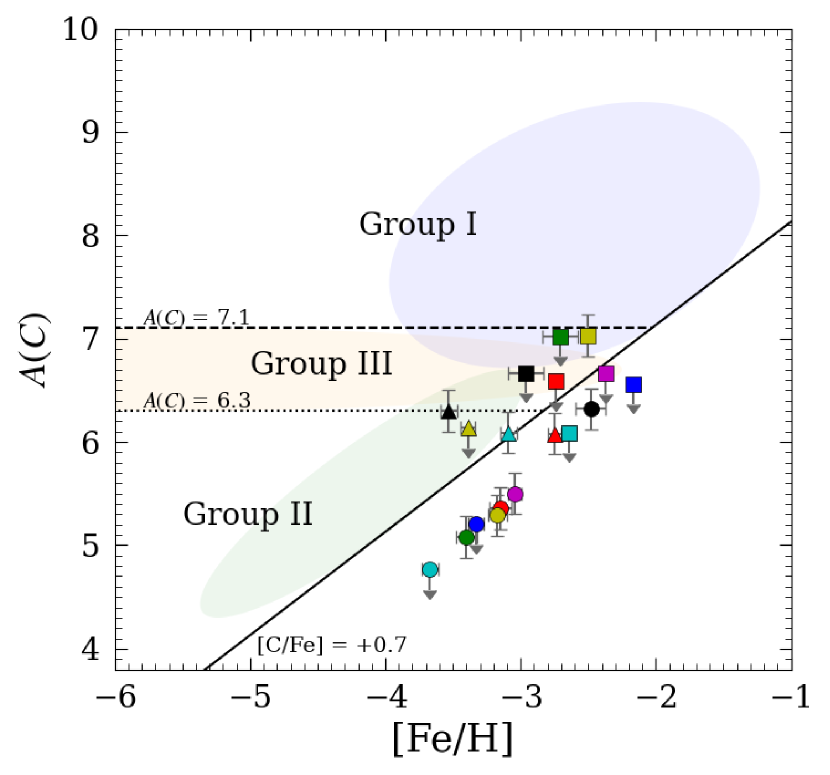
Figure 10: Yoon-Beers diagram of $A$(C) as a function of [Fe/H]. Light purple, green, and yellow circles indicate morphological Groups I, II, and III, respectively, as described by Yoon et al. (2016, 2019). The black solid, dashed, and dotted lines denote [C/Fe] = +0.7, $A$(C) = 7.1, and $A$(C) = 6.3, respectively. Note that the $A$(C) values are corrected for the evolutionary effects following the prescription of Placco et al. (2014). Their corrections are listed in Table 7 in the Appendix. The color and symbol are the same as in Figure 3. The down arrow indicates the upper limit estimate.

5.2 Carbon-Enhanced Metal-Poor (CEMP) Stars

Based on the [C/Fe] estimates of our program stars, three objects (excluding upper limit estimates) can be classified as CEMP stars ([C/Fe] $>$ +0.7), resulting in a CEMP fraction of 17% (3/18), which is not far from the literature value of $\sim$ 20% for [Fe/H] $<$ –2.0 (Lee et al., 2013; Placco et al., 2014). As they exhibit low Ba-abundance ratios ([Ba/Fe] $<$ 0.0), they are CEMP-$\rm no$ stars.

Previous studies reported that some CEMP (especially CEMP-no) stars are often enhanced with Na, Mg, Al, and Si (Norris et al., 2013; Aoki et al., 2018; Bonifacio et al., 2018). These characteristics can be useful to identify the mechanisms for the production of the CEMP stars. However, this is not the case for our CEMP stars, as they exhibit normal or relatively low abundance ratios of Na and Mg. In fact, only one potential CEMP object (J0758) with an upper limit of [C/Fe] = 1.2 exhibits a very low sodium ratio, [Na/Fe] = –0.75. The stars with peculiar abundances are mostly non-CEMP stars in our sample.

We have examined where our target stars are located in the $A$(C)-[Fe/H] diagram, the so-called Yoon-Beers Diagram, as shown in Figure 10. In the figure, the light purple, green, and yellow circles indicate the morphological regions for Group I, II, and III stars, respectively, as described by Yoon et al. (2016, 2019). The black solid, dashed, and dotted lines denote [C/Fe] = +0.7, $A$(C) = 7.1, and $A$(C) = 6.3, respectively. The legend for colors and symbols is the same as in Figure 3. The down arrow indicates an upper limit. Note that the $A$(C) values are corrected for the evolutionary effects following the prescription of Placco et al. (2014), and their uncorrected values and the amount of the correction are listed in Table 7 in the Appendix.

Inspection of Figure 10 reveals that, among our confirmed three CEMP stars, taking into account the low-metallicity ([Fe/H] $<$ –3.0) and $A$(C) level, two objects (black and cyan triangles) may belong to Group II, and one star (J1037, yellow square) with [Fe/H] $>$ –3.0 occupies Group I. According to the study by Yoon et al. (2016), stars in Group I are dominated by CEMP-$s$ or $r/s$ stars, which exhibit enhancements of $s$- or $r$-process elements (and may in fact be CEMP-$i$ stars), while Groups II and III contain mostly CEMP-no stars, which exhibit low abundance of neutron-capture elements. Considering its classification as CEMP-no star (due to their low Ba abundances), J1037 is likely to be in Group III rather than Group I. A recent study by Norris & Yong (2019) also reported that about 14% of the Group I CEMP objects belong to CEMP-no category. Since most of CEMP-$s$ stars show radial-velocity variation (e.g., Starkenburg et al., 2014; Placco et al., 2015b; Hansen et al., 2016a, b; Jorissen et al., 2016), indicative of their binarity, radial-velocity monitoring of these stars can further confirm their assigned CEMP sub-class.

As mentioned above, CEMP-no stars can be further sub-divided into two groups: one (Group II) with a good correlation between $A$(C) and [Fe/H], and the other (Group III) without clear correlation between them (Yoon et al., 2016). The fact that CEMP-no objects exhibit excesses in carbon with low neutron-capture elements implies that the sources of their chemical patterns are unlikely to be due to mass transfer from a binary companion, as in the CEMP-$s$ stars. Rather, they have likely been enriched through distinct nucleosynthesis channels. There are two channels of the formation of the CEMP-$\rm no$ stars that have been widely considered. One is pollution from faint SNe associated with Pop III stars. This type of SN experiences mixing and fallback (Umeda & Nomoto, 2003; Tominaga et al., 2007, 2014; Heger & Woosley, 2010; Nomoto et al., 2013; Ezzeddine et al., 2019), and ejects less iron due to its small explosion energy. Thus, only the outer layers, which have copious amounts of lighter elements, including carbon, are ejected, whereas the inner part, which includes a large amount of Fe falls back onto the neutron star or black hole, increasing the [C/Fe] ratio,

Another mechanism is a so-called spinstar. A rapidly rotating massive ultra metal-poor ([Fe/H] $<$ –4.0) star can have large amounts of carbon at its surface (due to efficient mixing with carbon production deeper in the star), and the surface material is blown by a stellar wind to pollute the ISM (Meynet et al., 2006; Hirschi, 2007; Frischknecht et al., 2012; Maeder et al., 2015). Additional formation mechanisms for CEMP-no stars are discussed in detail by Norris et al. (2013).

These two models cannot account completely for the observed chemical patterns of the CEMP-no stars. Nevertheless, one can infer from the different level of $A$(C) and the distinct behaviors in the $A$(Na)-$A$(C) and $A$(Mg)-$A$(C) spaces that the two Group II and Group III sub-groups may be associated with different formation mechanisms (Yoon et al., 2016). However, a much larger sample of CEMP-no stars (especially Group III stars) with accurate elemental-abundance estimates is required to better distinguish between these two channels. In this aspect, the CEMP-no stars identified through our work certainly help increase their sample size.

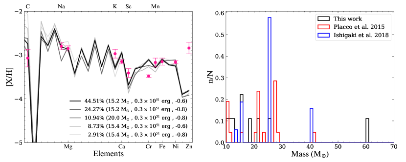
Figure 11: Left panel: Example of the abundance-pattern matching for J0713. Magenta symbols are the measured abundances. The solid lines represent the five best-fit models with different masses and mixing efficiencies. In this particular example, the explosion energy is the same for all five models. The percentage in the legend indicates the occurrence rate of the model among 10,000 predicted models. Right panel: Histogram (black) of the predicted progenitor masses of our EMP stars. The red and blue histograms are the mass distributions of the UMP stars predicted by Placco et al. (2015a) and the EMP stars derived by Ishigaki et al. (2018), respectively. Each histogram is normalized by the total number of stars to compare the mass distribution.

5.3 Chemically Peculiar Stars

5.3.1 Sodium-Peculiar Stars

In Figure 9, we identified one object (J0158) with [Na/Fe] = +1.14. This high Na-abundance ratio is a typical property of the second population (P2) in globular clusters (GCs). It is known that materials synthesized in stars of the primordial population (P1) of GCs, chemically enriched ISM with light elements such as Na and Al, so that the P2 stars exhibit distinct chemical characteristics from the P1 objects, establishing anti-correlations between Na-O and Al-Mg among stars in GCs (e.g., Gratton et al., 2004; Martell et al., 2011; Carretta et al., 2012; Pancino et al., 2017). This object thus may have originated in a GC.

Another piece of evidence for the chemical signature of a GC P2 in J0158 is its low Mg-abundance ratio, [Mg/Fe] = +0.06, yielding a very high [Na/Mg] ratio of +1.08. Its normal carbon content ([C/Fe] = +0.11) also points to P2, as P2 stars mostly exhibit normal to low values of carbon. Even though a further detailed abundance analysis is required, if this object is indeed a P2 star from a GC, such a cluster may once have belonged to a dwarf galaxy, because its metallicity ([Fe/H] = –3.04) is quite low compared to GCs in the MW. In line with this, Fernández-Trincado et al. (2017) argued that their low Mg-abundance stars with P2 chemical abundances could originate from outside of the MW. Additional kinematic study will help confirm whether or not it has been accreted from a dwarf satellite galaxy. We plan to carry out a thorough kinematics analysis of our program stars in a forthcoming paper.

The object J2242 is extremely Na poor ([Na/Fe] = –1.02); J1650 also has a relatively low [Na/Fe] = –0.6. However, both these stars are enhanced in K and Ni. As K is produced by CCSNe, and Ni is formed in the inner region of the explosion, it is plausible to infer that the gas clouds which formed these objects may have polluted by CCSNe with high explosion energies. Especially, considering its metallicity being [Fe/H] = –3.4, the progenitor of J2242 was unlikely to have been enriched by AGBs. Because the chemical abundances in the early MW were likely established by a limited number of chemical-enrichment events, this particular object may have undergone a peculiar nucleosynthesis episode. Its enhancement of K and Ni abundances supports the distinct nucleosynthesis hypothesis. However, recall that K and Ni for this star were only estimated from single absorption lines, thus additional high-resolution spectroscopic study of this object is necessary to confirm its peculiarity.

It is worthwhile mentioning that, in the case of globular clusters for NGC 2419 (Cohen & Kirby, 2012; Mucciarelli et al., 2012) and NGC 2808 (Mucciarelli et al., 2015), it has been reported that some of their member stars exhibit strong anti-correlations between their K and Mg abundance ratios. Kemp et al. (2018) also reported that a large number of their metal-poor stars selected from LAMOST are K rich, with relatively low Mg-abundance ratios, and concluded that an anomalous nucleosynthesis event might be associated with the progenitors of the stars. Even though the metallicities of our two K-rich objects are much lower than that of the stars from Kemp et al. (2018) ([Fe/H $>$ –1.5), because they are not strongly enhanced in Mg, they could belong to the same category.

5.3.2 Magnesium-Peculiar Stars

The object J0010 (black circle) in Figure 9 has [Mg/Fe] = +0.73, much higher than other halo stars near its metallicity ([Fe/H] = –2.48). This Mg-rich star is slightly enhanced with Na, while [Ca/Fe] looks normal (+0.19), resulting in an elevated [Mg/Ca] ratio (+0.54). The existence of the high-[Mg/Ca] objects has been suggested in numerous studies (Norris et al., 2002; Andrievsky et al., 2007; Frebel et al., 2008; Aoki et al., 2018). Its carbon enhancement is mild ([C/Fe] = +0.37). This star also stands out as a very low-Ba object with respect to other halo stars at [Fe/H] = –2.5; its [Ba/Fe] of –1.72 is over 1 dex lower than other objects at the same metallicity. Judging from its extremely low [Ba/Fe] ratio, this object may be not associated with events that produced large amounts of neutron-capture elements, but more likely with CCSNe, since most of its Ca and iron-peak show low or normal abundances, with the exception of Mn, whose abundance is uncertain due to weak Mn I lines.

J2241, indicated by the Mg-abundance plot of Figure 9, has [Mg/Fe] = –0.61, which is much lower than the other VMP stars near its metallicity ([Fe/H] = –2.71). Interestingly, this star’s Na-abundance ratio is also somewhat deficient with [Na/Fe] = –0.6. J1311 (red square) also has a relatively low [Mg/Fe], but nothing abnormal among the other abundances.

Mg-poor halo stars have also been reported in other studies (e.g., Ivans et al., 2003; Aoki et al., 2014). According to Ivans et al. (2003), the origin of these objects can be explained by larger pollution from SNe Ia compared to other halo objects with similar metallicities. Magnesium is primarily produced by massive stars, while Ca is created by both SNe Ia and CCSNe, resulting in a deficiency of Mg relative to Ca. Unfortunately, we do not have measured Ca abundances for the two low-[Mg/Fe] stars to confirm this scenario. Ivans et al. (2003) also reported very low [Na/Fe] and [Ba/Fe] ratios for their Mg-poor stars. One of our Mg-poor objects also exhibits this signature.

Stars with low $\alpha$-abundance ratios are sometimes explained by enhancement of their Fe (Cayrel et al., 2004; Yong et al., 2013; Jacobson et al., 2015). In this case, the abundance ratios of other elements are expected to be relatively lower as well. It will be worthwhile to carry out higher S/N, high-resolution follow-up observation for these low-[Mg/Fe] objects to see if other elements behave in this manner.

Another plausible explanation for the Mg-poor stars is that they came from classical or ultra-faint dwarf galaxies. These systems have had very low star-formation rates, and the contribution of SNe Ia started occurring at much lower metallicities (e.g., Shetrone et al., 2003; Tolstoy et al., 2009). In order to test this, a kinematic analysis of the Mg-deficient stars is presently being pursued.

Table 5: Predicted Progenitor Masses and SN Explosion Energies of Our EMP Stars

Short ID	Mass ($M_{\odot}$)	Energy (1051 erg)
J0102	10.9	0.9
J0158	21.0	0.3
J0422	60.0	3.0
J0713	15.2	0.3
J0758	11.9	0.9
J0814	25.5	0.9
J0908	12.8	0.3
J2242	18.6	10.0
J2341	15.2	0.3

Note. — Note that we did not attempt to determine the progenitor mass of the two reference stars (J0226 and J1522) and one program star (J0925), because only a few elements are available to constrain their progenitor mass.

5.4 Progenitor Masses of EMP Stars

Extremely metal-poor stars are regarded as fossil probes for understanding the chemical evolution of the early MW, because they preserve the chemical information of their natal gas clouds, permitting constraints on their predecessors, presumably massive Pop III stars. We explore the characteristics (especially mass and explosion energy) of the progenitors of our EMP stars by comparing their abundance patterns with theoretical predictions of Pop III SN models by Heger & Woosley (2010).

Their SN models consist of a grid of 16,800 combinations, which have a range of the explosion energy of 0.3 – 10 $\times$ $10^{51}$ erg and progenitor masses between of 10 – 100 $M_{\odot}$. There exist 120 initial masses, and the grid includes the mixing efficiencies from no mixing to nearly complete mixing. Using this grid, one can retrieve the progenitor properties of an EMP star by finding a best-matching SN chemical yield with the observed abundance patterns. We have made use of the starfit online tool to carry out this exercise. We only considered EMP stars among our program stars, and assumed that our EMP stars were formed out of the gas polluted by a single Pop III SN. If the measured abundance was derived from only one line, we treated it as upper limit, and we attempted to fit with all available abundances. In this exercise, we did not include the two reference stars (J0226 and J1522) and one program star (J0925), because the abundances of only a few elements are available for them to constrain their progenitor mass.

To confidently recover progenitor masses for our EMP stars, we generated 10,000 different abundance patterns by resampling each abundance from a normal error distribution for each object, obtaining distributions of masses and explosion energies of 10,000 possibilities. The left panel of Figure 11 shows an example of the best-matching chemical yield for J0713. The magenta symbols represent the observed abundances. Each solid line represents the theoretically predicted abundance patterns produced by a combination of different masses, explosion energies, and mixing efficiencies, as indicated in the legend at the top of the panel. In this particular example, all five best-fit models have the explosion energy of 0.3 $\times$ $10^{51}$ erg, and the best-fit model has a mass of 15.2 $M_{\odot}$ with mixing efficiency of –0.6, which accounts for 44.5% among 10,000 predicted models. The other four top models are followed with a range of masses, 15 – 20 $M_{\odot}$ and mixing efficiency of –0.6 or –0.8. We chose the most frequently occurring model, and adopted its mass as the progenitor mass of our EMP star.

The right panel of Figure 11 displays a histogram of the predicted progenitor masses of our EMP stars. The histogram implies that except one object (60 $M_{\odot}$), our EMP objects have a progenitor mass of less than 26 $M_{\odot}$. Table 5 lists the most probable masses and explosion energies for our EMP stars.

Placco et al. (2015a) used the same SNe models by Heger & Woosley (2010) to determine the progenitor masses of 21 UMP stars, and found that most of their progenitors have the mass range 20 – 28 $M_{\odot}$ and explosion energies 0.3 – 0.9 $\times$ $10^{51}$ erg (see also Placco et al. 2016 for the progenitor masses of additional UMP stars). The red histogram of the right panel of Figure 11 is their mass estimates of the UMP progenitors, which are mostly less than 40 $M_{\odot}$. The mass range of our EMP stars is somewhat less than that of Placco et al. (2015a), but generally in good agreement. The majority of our EMP stars have their progenitor SN explosion energy between 0.3 and 1.0 $\times$ $10^{51}$ erg, as can be read off from Table 5, again consistent with that of Placco et al. (2015a). Placco et al. pointed out that the estimated mass and explosion energy are very sensitive to the present of carbon and nitrogen abundance. The relatively lower masses of our EMP progenitors compared to theirs may thus be due to the absence of the measured N abundance for our EMP stars.

Ishigaki et al. (2018) also carried out a similar work to derive the mass function of the first stars, using about 200 EMP stars, but with different SN models. They used mixing and fallback SNe models, which have the combination of five initial masses (13, 15, 25, 40, and 100 $M_{\odot}$) and explosion energies of 0.5, 1.0, 10, 30, and 60 $\times$ $10^{51}$ erg to represent low-, normal-, and high-energy explosions. They found that the progenitor masses of their sample are mostly less than 40 $M_{\odot}$, as can be seen in the blue histogram of the right panel of Figure 11. Our predicted masses also agree well with theirs. They also suggested that the C, N, and O abundances are sensitive to the progenitor mass, and that the Na, Mg, and Al abundance ratios are also useful tracers of the progenitor mass when ignoring the impact of stellar rotation.

To sum up, the (relatively) low-mass range of the progenitors of our sample and other studies suggests that stars with $M<$ 40 $M_{\odot}$were likely primarily responsible for the chemical enrichment of the early MW.

6 Summary and Future Work

We have carried out high-resolution spectroscopic follow-up observations using GEMINI-N/GRACES for 20 stars (including two reference stars), selected as EMP candidates from SDSS and LAMOST medium-resolution spectra. We have presented stellar parameters and abundance estimates for Li, C, Na, Mg, K, Ca, Sc, Cr, Mn, Fe, Ni, Zn, and Ba, which are derived from a 1D LTE abundance analysis. The chemical abundances of our EMP candidates are compared with those of two benchmark stars from previous studies, and they show good agreement, validating our measurements of the program star chemical abundances.

Based on our chemical abundances, we have found that all our candidates are VMP stars, and include 10 objects that are EMP stars. In addition, three CEMP stars are newly identified, and their low-Ba abundances ([Ba/Fe] $<$ 0.0) indicate that they are all CEMP-$\rm no$ objects. As a result, our work nicely contributes to increasing the sample size of the VMP/EMP stars as well as CEMP-no objects.

The Li abundance of our warm dwarf is slightly lower than the Spite Plateau, possibly due to the different temperature scale adopted. On the other hand, the $A$(Li) values of our TO stars are distributed around the Spite Plateau. Consequently, they can be used to constrain the Spite plateau by follow-up studies, and especially, the TO stars may contribute to extending the Spite plateau to the warmer temperature region.

Comparison with other Galactic halo VMP stars reveals that the chemical abundances of our VMP objects generally follow similar abundance trends as a function of [Fe/H]. However, there exist a few objects that stand out from the majority of the VMP stars. We have identified one star (J0158) with [Na/Fe] = +1.14. Its low [Fe/H], [Mg/Fe], and [C/Fe] values imply that this object is closely connected to a second-generation star from a GC that once belonged to a dwarf galaxy. The object J2242 has an extremely low-sodium abundance ratio of [Na/Fe] = –1.02. This object also exhibits enhancement of K and Ni abundances. Taking into account its metallicity of [Fe/H] = –3.4, this star may have formed in a gas cloud that was chemically enriched by CCSNe with high explosion energies.

We also found a Mg-rich star ([Mg/Fe] = +0.73) that is also slightly enhanced with Na, while its [Ca/Fe] is normal. These abundance characteristics, together with the extremely low [Ba/Fe], suggest that this VMP star is not likely to be associated with CCSNe that produce a large amount of neutron-capture elements. The star J2241 exhibits the lowest [Mg/Fe] (–0.61). The origin of this Mg-poor star can be explained by larger pollution by SNe Ia, or it could be accreted from a dwarf galaxy that experienced low star-formation efficiency.

We have also explored the progenitor characteristics (mass and explosion energy) of our EMP stars by comparing their chemical-abundance patterns with those predicted by Pop III SN models. Except one object (60 $M_{\odot}$), our estimate masses of the EMP stars are in the range of 10 – 26 $M_{\odot}$, which is in good agreement with the previous studies by Placco et al. (2015a) and Ishigaki et al. (2018). This suggests that the chemical evolution of the early MW was driven primarily by stars with masses $M<$ 40 $M_{\odot}$.

Since there are some uncertainties in the derived abundance for some elements due to weak metallic lines, low-S/N spectra, or a small number of measured lines, we plan to carry out high-resolution, high-S/N spectroscopic observations for the chemically peculiar objects to determine more reliable measurements of their elemental abundances. We also plan to supplement the available chemical information for our program stars with a chemodynamical analysis in an upcoming paper.

Table 6 lists the line information used to derived chemical abundances. The carbon abundance ratios and their corrected value according to the evolutionary stage are listed in Table 7. Table 8 provides detailed abundance measurements of other elements and their associated errors.

Table 6: Line Lists

Species	Wavelength (Å)	EP (eV)	log $gf$
3.0	6707.70	0.00	0.17
11.0	5895.92	0.00	–0.19
11.0	5889.95	0.00	0.11
12.0	5528.41	4.34	–0.50
12.0	5183.60	2.72	–0.24
12.0	4702.99	4.33	–0.38
12.0	5172.68	2.71	–0.45
19.0	7664.90	0.00	0.14
19.0	7698.96	0.00	–0.17
20.0	5262.24	2.52	–0.47
20.0	5265.56	2.52	–0.26
20.0	5349.47	2.71	–0.31
20.0	5588.76	2.52	0.21
20.0	6493.79	2.52	–0.11
20.0	6462.57	2.52	0.26
20.0	6102.72	1.88	–0.79
20.0	6122.22	1.89	–0.32
20.0	6162.17	1.90	–0.09
20.0	6439.07	2.52	0.47
20.0	5598.49	2.52	–0.09
20.0	5594.47	2.52	0.10
21.1	5318.37	1.36	–2.01
21.1	5031.01	1.36	–0.40
21.1	5657.91	1.51	–0.60
21.1	5526.79	1.77	0.02
21.1	5239.81	1.46	–0.77
22.0	4840.87	0.90	–0.45
22.0	4991.07	0.84	0.44
22.0	4981.73	0.84	0.56
22.0	5192.97	0.02	–0.95
22.0	5210.39	0.05	–0.83
22.0	5064.65	0.05	–0.94
22.0	5007.21	0.82	0.17
22.0	5024.84	0.82	–0.55
22.0	5009.65	0.02	–2.20
22.0	5039.96	0.02	–1.13
22.0	5014.19	0.00	–1.22
22.0	5014.28	0.81	0.11
22.0	5038.40	1.43	0.07
22.0	5016.16	0.85	–0.52
22.0	5036.46	1.44	0.19
22.0	5035.90	1.46	0.26
22.0	5020.02	0.84	–0.36
22.0	5173.74	0.00	–1.06
22.0	4999.50	0.83	0.31
24.0	5296.69	0.98	–1.36
24.0	5409.77	1.03	–0.67
24.0	4789.34	2.54	–0.33
24.0	5206.04	0.94	0.02
24.0	5348.31	1.00	–1.21
24.0	5345.80	1.00	–0.95
24.0	5247.56	0.96	–1.64
24.0	5208.42	0.94	0.16
24.0	5300.74	0.98	–2.00
24.0	5298.28	0.98	–1.14
25.0	4783.43	2.30	0.04
25.0	4754.05	2.28	–0.09
25.0	4823.53	2.32	0.14
26.0	5379.57	3.69	–1.51
26.0	5383.37	4.31	0.65
26.0	5027.23	3.64	–1.89
26.0	5389.48	4.42	–0.41
26.0	5322.04	2.28	–2.80
26.0	5397.13	0.92	–1.98
26.0	5405.78	0.99	–1.85
26.0	5288.53	3.68	–1.51
26.0	5410.91	4.47	0.40
26.0	5415.20	4.39	0.64
26.0	4920.50	2.83	0.07
26.0	5393.17	3.24	–0.91
26.0	5371.49	0.96	–1.64
26.0	5367.47	4.42	0.44
26.0	5307.36	1.61	–2.91
26.0	5365.40	3.56	–1.02
26.0	5424.07	4.32	0.52
26.0	5364.87	4.45	0.23
26.0	4800.65	4.12	–1.03
26.0	5302.30	3.28	–0.72
26.0	5339.93	3.27	–0.72
26.0	4924.77	2.28	–2.11
26.0	5332.90	1.55	–2.78
26.0	5328.53	1.56	–1.85
26.0	5328.04	0.92	–1.47
26.0	5324.18	3.21	–0.10
26.0	5369.96	4.37	0.54
26.0	5429.70	0.96	–1.88
26.0	5446.92	0.99	–1.91
26.0	5283.62	3.24	–0.52
26.0	6137.69	2.59	–1.35
26.0	4736.77	3.21	–0.75
26.0	6191.56	2.43	–1.42
26.0	6230.72	2.56	–1.28
26.0	6252.56	2.4	–1.69
26.0	6297.79	2.22	–2.64
26.0	6393.60	2.43	–1.58
26.0	6400.00	3.6	–0.29
26.0	6430.85	2.18	–1.95
26.0	4733.59	1.49	–2.99
26.0	6494.98	2.40	–1.24
26.0	6677.99	2.69	–1.42
26.0	4710.28	3.02	–1.61
26.0	4871.32	2.87	–0.36
26.0	4707.27	3.24	–1.08
26.0	6136.62	2.45	–1.41
26.0	4872.14	2.88	–0.57
26.0	6065.48	2.61	–1.41
26.0	4890.76	2.88	–0.39
26.0	5455.61	1.01	–2.09
26.0	5497.52	1.01	–2.83
26.0	5501.46	0.96	–3.05
26.0	5506.78	0.99	–2.79
26.0	4918.99	2.85	–0.34
26.0	5572.84	3.40	–0.28
26.0	5586.76	3.37	–0.14
26.0	5434.52	1.01	–2.13
26.0	4789.65	3.53	–0.96
26.0	5615.64	3.33	0.05
26.0	5624.54	3.42	–0.76
26.0	4903.31	2.88	–0.93
26.0	5662.52	4.18	–0.57
26.0	5686.53	4.55	–0.45
26.0	5753.12	4.26	–0.69
26.0	4891.49	2.85	–0.11
26.0	4786.81	3.00	–1.61
26.0	5281.79	3.04	–0.83
26.0	5028.13	3.56	–1.12
26.0	5150.84	0.99	–3.04
26.0	5110.41	0.00	–3.76
26.0	5123.72	1.01	–3.06
26.0	5125.12	4.22	–0.14
26.0	5127.36	0.92	–3.25
26.0	5001.87	3.88	0.05
26.0	5131.47	2.22	–2.52
26.0	5098.70	2.18	–2.03
26.0	5133.69	4.18	0.14
26.0	5141.74	2.42	–2.24
26.0	5142.93	0.96	–3.08
26.0	5269.54	0.86	–1.33
26.0	5151.91	1.01	–3.32
26.0	5162.27	4.18	0.02
26.0	5166.28	0.00	–4.12
26.0	5137.38	4.18	–0.40
26.0	5171.60	1.49	–1.72
26.0	5090.77	4.26	–0.36
26.0	5080.95	3.27	–3.09
26.0	5022.24	3.98	–0.53
26.0	5014.94	3.94	–0.30
26.0	5012.07	0.86	–2.64
26.0	5041.07	0.96	–3.09
26.0	5041.76	1.49	–2.20
26.0	5044.21	2.85	–2.02
26.0	5083.34	0.96	–2.84
26.0	5049.82	2.28	–1.36
26.0	5060.08	0.00	–5.46
26.0	5006.12	2.83	–0.62
26.0	5068.77	2.94	–1.04
26.0	5074.75	4.22	–0.20
26.0	5079.22	2.20	–2.11
26.0	5079.74	0.99	–3.25
26.0	5051.63	0.92	–2.76
26.0	4994.13	0.92	–2.97
26.0	5227.19	1.56	–1.23
26.0	4957.60	2.81	0.23
26.0	5204.58	0.09	–4.33
26.0	5250.21	0.12	–4.94
26.0	5216.27	1.61	–2.08
26.0	5217.39	3.21	–1.16
26.0	5225.53	0.11	–4.76
26.0	4957.30	2.85	–0.41
26.0	5202.34	2.18	–1.87
26.0	4859.74	2.88	–0.76
26.0	4939.69	0.86	–3.25
26.0	4946.39	3.37	–1.17
26.0	5263.31	3.27	–0.88
26.0	5242.49	3.63	–0.97
26.0	5247.05	0.09	–4.95
26.0	5254.96	0.11	–4.76
26.0	5232.94	2.94	–0.06
26.0	5266.56	3.00	–0.39
26.0	5250.65	2.20	–2.18
26.0	5198.71	2.22	–2.09
26.0	5194.94	1.56	–2.02
26.0	4938.81	2.88	–1.08
26.0	4973.10	3.96	–0.95
26.0	4966.09	3.33	–0.87
26.0	5191.46	3.04	–0.55
26.0	5192.34	3.00	–0.42
28.0	5017.59	3.54	–0.08
28.0	5035.37	3.63	0.29
28.0	4714.42	3.38	0.23
28.0	4980.16	3.61	–0.11
28.0	5080.52	3.65	0.13
28.0	5081.11	3.85	0.30
28.0	5084.08	3.68	0.03
28.0	5115.40	3.83	–0.11
28.0	5578.73	1.68	–2.64
28.0	5137.08	1.68	–1.99
28.0	4904.41	3.54	–0.17
28.0	5476.90	1.83	–0.89
28.0	5155.76	3.90	–0.09
28.0	4855.41	3.54	0.00
28.0	5754.68	1.94	–2.33
30.0	4810.53	4.08	–0.14
30.0	4722.15	4.03	–0.39
56.1	6496.90	0.60	–0.38
56.1	4934.09	0.00	–0.16

Note. — EP is the excitation potential.

Table 7: Carbon-Abundance Ratios and Their Corrections for Evolutionary Stage

Short ID	[C/Fe]BC	Ccor	[C/Fe]	$A$(C)
J0010	–0.22	0.59	0.37	6.32
J0102	0.75	0.00	0.75	6.09
J0158	0.10	0.01	0.11	5.50
J0226	1.33	0.00	1.33	5.98
J0357	0.40	0.00	0.40	6.08
J0422	$<$0.10	0.01	$<$0.11	$<$5.21
J0713	–0.60	0.68	0.08	5.36
J0758	$<$1.20	0.00	$<$1.20	$<$6.67
J0814	$<$1.10	0.00	$<$1.10	$<$6.14
J0908	$<$–0.40	0.41	$<$0.01	$<$4.77
J0925	1.40	0.00	1.40	6.30
J1037	1.10	0.00	1.10	7.03
J1311	$<$0.90	0.00	$<$0.90	$<$6.59
J1317	$<$0.60	0.00	$<$0.60	$<$6.66
J1522	$<$1.03	0.00	$<$1.03	$<$5.76
J1650	$<$0.30	0.00	$<$0.30	$<$6.56
J1705	$<$0.30	0.00	$<$0.30	$<$6.09
J2241	$<$1.30	0.00	$<$1.30	$<$7.02
J2242	–0.20	0.25	0.05	5.08
J2341	–0.50	0.53	0.03	5.29

Note. — C_cor indicates the amount of correction following Placco et al. (2014) due to the evolution status. [C/Fe]_BC is the value before C_cor is applied, while [C/Fe] and $A$(C) are the values after the correction is applied. The $<$ symbol indicates an upper limit estimate. As mentioned in Section 4.2, the measured error is conservatively assumed to be 0.2 dex.

Table 8: Detailed Chemical Abundances for Each Object

Species	$N$	$\log\epsilon$ (X)	[X/Fe]	SE	$\Delta$$T_{\rm eff}$	$\Delta$$\log~{}g$	$\Delta$$\xi_{\rm t}$	TE
				(dex)	$\pm$100 K	$\pm$0.2 dex	$\pm$0.2 km s-1	(dex)
J0010
Li I	$\cdots$	$\cdots$	$\cdots$	$\cdots$	$\cdots$	$\cdots$	$\cdots$	$\cdots$
Na I	2	4.00	0.24	0.12	0.06	0.00	0.04	0.07
Mg I	4	5.85	0.73	0.02	0.06	0.05	0.02	0.04
K I	1	2.68	0.13	0.17	0.03	0.02	0.07	0.09
Ca I	12	4.05	0.19	0.06	0.06	0.00	0.05	0.05
Sc II	4	0.34	–0.33	0.06	0.18	0.09	0.07	0.11
Cr I	9	3.06	–0.10	0.08	0.05	0.00	0.02	0.05
Mn I	3	3.04	0.09	0.10	0.02	0.04	0.02	0.06
Fe I	121	5.02	0.00	0.02	0.18	0.06	0.10	0.11
Ni I	13	3.87	0.13	0.03	0.07	0.01	0.07	0.05
Zn I	2	2.08	0.00	0.12	0.20	0.04	0.08	0.12
Ba II	2	–2.02	–1.72	0.06	$\cdots$	$\cdots$	$\cdots$	0.06
J0102
Li I	1	1.75	3.79	0.20	$\cdots$	$\cdots$	$\cdots$	0.20
Na I	2	2.55	–0.60	0.23	0.02	0.01	0.01	0.12
Mg I	2	4.72	0.21	0.23	0.01	0.07	0.01	0.12
K I	$\cdots$	$\cdots$	$\cdots$	$\cdots$	$\cdots$	$\cdots$	$\cdots$	$\cdots$
Ca I	$\cdots$	$\cdots$	$\cdots$	$\cdots$	$\cdots$	$\cdots$	$\cdots$	$\cdots$
Sc II	$\cdots$	$\cdots$	$\cdots$	$\cdots$	$\cdots$	$\cdots$	$\cdots$	$\cdots$
Cr I	1	2.51	–0.04	0.33	0.01	0.01	0.01	0.17
Mn I	$\cdots$	$\cdots$	$\cdots$	$\cdots$	$\cdots$	$\cdots$	$\cdots$	$\cdots$
Fe I	13	4.41	0.00	0.09	0.08	0.0	0.02	0.06
Ni I	$\cdots$	$\cdots$	$\cdots$	$\cdots$	$\cdots$	$\cdots$	$\cdots$	$\cdots$
Zn I	$\cdots$	$\cdots$	$\cdots$	$\cdots$	$\cdots$	$\cdots$	$\cdots$	$\cdots$
Ba II	$\cdots$	$\cdots$	$\cdots$	$\cdots$	$\cdots$	$\cdots$	$\cdots$	$\cdots$
J0158
Li I	1	0.79	2.78	0.20	$\cdots$	$\cdots$	$\cdots$	0.20
Na I	2	4.34	1.14	0.13	0.02	0.06	0.05	0.08
Mg I	4	4.62	0.06	0.11	0.03	0.02	0.02	0.06
K I	$\cdots$	$\cdots$	$\cdots$	$\cdots$	$\cdots$	$\cdots$	$\cdots$	$\cdots$
Ca I	8	3.71	0.41	0.08	0.04	0.00	0.01	0.04
Sc II	$\cdots$	$\cdots$	$\cdots$	$\cdots$	$\cdots$	$\cdots$	$\cdots$	$\cdots$
Cr I	3	2.51	–0.09	0.11	0.00	0.00	0.00	0.06
Mn I	1	2.38	–0.01	0.19	0.02	0.00	0.02	0.10
Fe I	62	4.46	–0.00	0.02	0.10	0.01	0.02	0.05
Ni I	3	3.48	0.30	0.11	0.02	0.01	0.02	0.06
Zn I	1	2.13	0.61	0.19	0.06	0.04	0.02	0.10
Ba II	1	$<$–2.46	$<$–1.60	0.20	$\cdots$	$\cdots$	$\cdots$	0.20
J0226
Li I	$\cdots$	$\cdots$	$\cdots$	$\cdots$	$\cdots$	$\cdots$	$\cdots$	$\cdots$
Na I	2	2.75	0.29	0.07	0.02	0.01	0.01	0.04
Mg I	2	4.41	0.59	0.07	0.02	0.02	0.07	0.05
K I	$\cdots$	$\cdots$	$\cdots$	$\cdots$	$\cdots$	$\cdots$	$\cdots$	$\cdots$
Ca I	$\cdots$	$\cdots$	$\cdots$	$\cdots$	$\cdots$	$\cdots$	$\cdots$	$\cdots$
Sc II	$\cdots$	$\cdots$	$\cdots$	$\cdots$	$\cdots$	$\cdots$	$\cdots$	$\cdots$
Cr I	$\cdots$	$\cdots$	$\cdots$	$\cdots$	$\cdots$	$\cdots$	$\cdots$	$\cdots$
Mn I	$\cdots$	$\cdots$	$\cdots$	$\cdots$	$\cdots$	$\cdots$	$\cdots$	$\cdots$
Fe I	15	3.72	0.00	0.03	0.10	0.01	0.01	0.05
Ni I	$\cdots$	$\cdots$	$\cdots$	$\cdots$	$\cdots$	$\cdots$	$\cdots$	$\cdots$
Zn I	$\cdots$	$\cdots$	$\cdots$	$\cdots$	$\cdots$	$\cdots$	$\cdots$	$\cdots$
Ba II	$\cdots$	$\cdots$	$\cdots$	$\cdots$	$\cdots$	$\cdots$	$\cdots$	$\cdots$
J0357
Li I	1	1.83	3.53	0.20	$\cdots$	$\cdots$	$\cdots$	0.20
Na I	2	3.62	0.13	0.13	0.01	0.03	0.03	0.07
Mg I	4	5.19	0.34	0.06	0.01	0.04	0.01	0.04
K I	$\cdots$	$\cdots$	$\cdots$	$\cdots$	$\cdots$	$\cdots$	$\cdots$	$\cdots$
Ca I	8	3.92	0.33	0.05	0.03	0.01	0.02	0.03
Sc II	1	0.90	0.50	0.18	0.06	0.07	0.02	0.10
Cr I	3	2.73	–0.16	0.10	0.01	0.01	0.01	0.05
Mn I	1	2.69	0.01	0.18	0.02	0.00	0.02	0.09
Fe I	64	4.75	0.00	0.02	0.09	0.00	0.02	0.05
Ni I	2	3.84	0.37	0.13	0.02	0.01	0.01	0.07
Zn I	1	2.62	0.81	0.18	0.05	0.03	0.02	0.10
Ba II	2	–1.27	–0.70	0.04	$\cdots$	$\cdots$	$\cdots$	0.04
J0422
Li I	$\cdots$	$\cdots$	$\cdots$	$\cdots$	$\cdots$	$\cdots$	$\cdots$	$\cdots$
Na I	2	2.45	–0.46	0.15	0.02	0.00	0.01	0.08
Mg I	4	4.45	0.18	0.06	0.04	0.00	0.03	0.04
K I	$\cdots$	$\cdots$	$\cdots$	$\cdots$	$\cdots$	$\cdots$	$\cdots$	$\cdots$
Ca I	5	3.22	0.21	0.08	0.04	0.00	0.02	0.05
Sc II	$\cdots$	$\cdots$	$\cdots$	$\cdots$	$\cdots$	$\cdots$	$\cdots$	$\cdots$
Cr I	2	1.95	–0.36	0.15	0.01	0.00	0.01	0.08
Mn I	$\cdots$	$\cdots$	$\cdots$	$\cdots$	$\cdots$	$\cdots$	$\cdots$	$\cdots$
Fe I	54	4.17	0.00	0.03	0.12	0.01	0.02	0.06
Ni I	2	3.12	0.23	0.15	0.03	0.00	0.02	0.08
Zn I	$\cdots$	$\cdots$	$\cdots$	$\cdots$	$\cdots$	$\cdots$	$\cdots$	$\cdots$
Ba II	2	–2.30	–1.15	0.20	$\cdots$	$\cdots$	$\cdots$	0.20
J0713
Li I	$\cdots$	$\cdots$	$\cdots$	$\cdots$	$\cdots$	$\cdots$	$\cdots$	$\cdots$
Na I	2	3.45	0.37	0.13	0.06	0.01	0.06	0.08
Mg I	4	4.75	0.31	0.10	0.05	0.02	0.02	0.06
K I	1	2.05	0.18	0.19	0.05	0.03	0.04	0.10
Ca I	8	3.18	0.00	0.02	0.08	0.03	0.04	0.05
Sc II	3	–0.27	–0.26	0.11	0.14	0.10	0.04	0.10
Cr I	5	2.15	–0.33	0.06	0.02	0.00	0.01	0.03
Mn I	1	2.25	–0.02	0.19	0.08	0.00	0.03	0.10
Fe I	96	4.34	0.00	0.02	0.15	0.06	0.04	0.08
Ni I	4	3.05	–0.01	0.04	0.07	0.01	0.03	0.04
Zn I	1	1.71	0.31	0.19	0.16	0.04	0.04	0.13
Ba II	2	–2.66	–2.08	0.04	$\cdots$	$\cdots$	$\cdots$	0.04
J0758
Li I	$\cdots$	$\cdots$	$\cdots$	$\cdots$	$\cdots$	$\cdots$	$\cdots$	$\cdots$
Na I	1	2.53	–0.75	0.47	0.02	0.01	0.01	0.24
Mg I	2	4.70	0.06	0.33	0.02	0.02	0.03	0.17
K I	$\cdots$	$\cdots$	$\cdots$	$\cdots$	$\cdots$	$\cdots$	$\cdots$	$\cdots$
Ca I	$\cdots$	$\cdots$	$\cdots$	$\cdots$	$\cdots$	$\cdots$	$\cdots$	$\cdots$
Sc II	$\cdots$	$\cdots$	$\cdots$	$\cdots$	$\cdots$	$\cdots$	$\cdots$	$\cdots$
Cr I	1	2.57	–0.11	0.47	0.01	0.00	0.01	0.24
Mn I	$\cdots$	$\cdots$	$\cdots$	$\cdots$	$\cdots$	$\cdots$	$\cdots$	$\cdots$
Fe I	4	4.54	0.00	0.24	0.08	0.00	0.00	0.13
Ni I	$\cdots$	$\cdots$	$\cdots$	$\cdots$	$\cdots$	$\cdots$	$\cdots$	$\cdots$
Zn I	$\cdots$	$\cdots$	$\cdots$	$\cdots$	$\cdots$	$\cdots$	$\cdots$	$\cdots$
Ba II	$\cdots$	$\cdots$	$\cdots$	$\cdots$	$\cdots$	$\cdots$	$\cdots$	$\cdots$
J0814
Li I	1	1.76	4.10	0.20	$\cdots$	$\cdots$	$\cdots$	0.20
Na I	2	2.80	–0.05	0.10	0.02	0.00	0.00	0.05
Mg I	3	4.54	0.33	0.08	0.03	0.02	0.02	0.04
K I	$\cdots$	$\cdots$	$\cdots$	$\cdots$	$\cdots$	$\cdots$	$\cdots$	$\cdots$
Ca I	1	3.56	0.61	0.14	0.04	0.01	0.01	0.07
Sc II	$\cdots$	$\cdots$	$\cdots$	$\cdots$	$\cdots$	$\cdots$	$\cdots$	$\cdots$
Cr I	$\cdots$	$\cdots$	$\cdots$	$\cdots$	$\cdots$	$\cdots$	$\cdots$	$\cdots$
Mn I	$\cdots$	$\cdots$	$\cdots$	$\cdots$	$\cdots$	$\cdots$	$\cdots$	$\cdots$
Fe I	13	4.11	0.00	0.04	0.10	0.00	0.02	0.05
Ni I	$\cdots$	$\cdots$	$\cdots$	$\cdots$	$\cdots$	$\cdots$	$\cdots$	$\cdots$
Zn I	$\cdots$	$\cdots$	$\cdots$	$\cdots$	$\cdots$	$\cdots$	$\cdots$	$\cdots$
Ba II	$\cdots$	$\cdots$	$\cdots$	$\cdots$	$\cdots$	$\cdots$	$\cdots$	$\cdots$
J0908
Li I	$\cdots$	$\cdots$	$\cdots$	$\cdots$	$\cdots$	$\cdots$	$\cdots$	$\cdots$
Na I	2	2.38	–0.19	0.15	0.02	0.01	0.02	0.08
Mg I	3	4.10	0.17	0.12	0.06	0.01	0.04	0.07
K I	1	2.32	0.96	0.21	0.04	0.02	0.02	0.11
Ca I	4	3.02	0.35	0.07	0.05	0.01	0.02	0.04
Sc II	$\cdots$	$\cdots$	$\cdots$	$\cdots$	$\cdots$	$\cdots$	$\cdots$	$\cdots$
Cr I	2	1.50	–0.47	0.15	0.01	0.01	0.02	0.08
Mn I	$\cdots$	$\cdots$	$\cdots$	$\cdots$	$\cdots$	$\cdots$	$\cdots$	$\cdots$
Fe I	49	3.83	0.00	0.03	0.12	0.02	0.03	0.06
Ni I	2	2.90	0.35	0.15	0.03	0.00	0.02	0.08
Zn I	$\cdots$	$\cdots$	$\cdots$	$\cdots$	$\cdots$	$\cdots$	$\cdots$	$\cdots$
Ba II	1	$<$–2.89	$<$–1.40	0.20	$\cdots$	$\cdots$	$\cdots$	0.20
J0925
Li I	1	1.32	3.80	0.20	$\cdots$	$\cdots$	$\cdots$	0.20
Mg I	2	4.42	0.35	0.09	0.02	0.02	0.05	0.05
K I	$\cdots$	$\cdots$	$\cdots$	$\cdots$	$\cdots$	$\cdots$	$\cdots$	$\cdots$
Ca I	$\cdots$	$\cdots$	$\cdots$	$\cdots$	$\cdots$	$\cdots$	$\cdots$	$\cdots$
Sc II	$\cdots$	$\cdots$	$\cdots$	$\cdots$	$\cdots$	$\cdots$	$\cdots$	$\cdots$
Cr I	$\cdots$	$\cdots$	$\cdots$	$\cdots$	$\cdots$	$\cdots$	$\cdots$	$\cdots$
Mn I	$\cdots$	$\cdots$	$\cdots$	$\cdots$	$\cdots$	$\cdots$	$\cdots$	$\cdots$
Fe I	7	3.97	0.00	0.05	0.11	0.00	0.02	0.06
Ni I	$\cdots$	$\cdots$	$\cdots$	$\cdots$	$\cdots$	$\cdots$	$\cdots$	$\cdots$
Zn I	$\cdots$	$\cdots$	$\cdots$	$\cdots$	$\cdots$	$\cdots$	$\cdots$	$\cdots$
Ba II	$\cdots$	$\cdots$	$\cdots$	$\cdots$	$\cdots$	$\cdots$	$\cdots$	$\cdots$
J1037
Li I	1	2.21	3.66	0.20	$\cdots$	$\cdots$	$\cdots$	0.20
Na I	2	3.33	–0.41	0.12	0.01	0.01	0.01	0.06
Mg I	4	5.40	0.30	0.05	0.02	0.03	0.01	0.03
K I	$\cdots$	$\cdots$	$\cdots$	$\cdots$	$\cdots$	$\cdots$	$\cdots$	$\cdots$
Ca I	4	3.96	0.12	0.04	0.03	0.01	0.02	0.03
Cr I	1	2.90	–0.24	0.17	0.01	0.00	0.01	0.09
Mn I	$\cdots$	$\cdots$	$\cdots$	$\cdots$	$\cdots$	$\cdots$	$\cdots$	$\cdots$
Fe I	21	5.00	0.00	0.04	0.08	0.0	0.02	0.05
Ni I	1	4.06	0.34	0.17	0.01	0.0	0.01	0.09
Zn I	$\cdots$	$\cdots$	$\cdots$	$\cdots$	$\cdots$	$\cdots$	$\cdots$	$\cdots$
Ba II	$\cdots$	$\cdots$	$\cdots$	$\cdots$	$\cdots$	$\cdots$	$\cdots$	$\cdots$
J1311
Li I	$\cdots$	$\cdots$	$\cdots$	$\cdots$	$\cdots$	$\cdots$	$\cdots$	$\cdots$
Na I	1	3.38	–0.12	0.05	0.02	0.01	0.02	0.03
Mg I	2	4.64	–0.22	0.04	0.02	0.02	0.03	0.03
K I	$\cdots$	$\cdots$	$\cdots$	$\cdots$	$\cdots$	$\cdots$	$\cdots$	$\cdots$
Ca I	$\cdots$	$\cdots$	$\cdots$	$\cdots$	$\cdots$	$\cdots$	$\cdots$	$\cdots$
Sc II	$\cdots$	$\cdots$	$\cdots$	$\cdots$	$\cdots$	$\cdots$	$\cdots$	$\cdots$
Cr I	2	2.55	–0.35	0.04	0.00	0.00	0.00	0.02
Mn I	$\cdots$	$\cdots$	$\cdots$	$\cdots$	$\cdots$	$\cdots$	$\cdots$	$\cdots$
Fe I	2	4.76	0.00	0.04	0.08	0.00	0.01	0.04
Ni I	$\cdots$	$\cdots$	$\cdots$	$\cdots$	$\cdots$	$\cdots$	$\cdots$	$\cdots$
Zn I	$\cdots$	$\cdots$	$\cdots$	$\cdots$	$\cdots$	$\cdots$	$\cdots$	$\cdots$
Ba II	1	$<$–0.76	$<$–0.2	0.20	$\cdots$	$\cdots$	$\cdots$	0.20
J1317
Li I	1	2.41	3.73	0.20	$\cdots$	$\cdots$	$\cdots$	0.20
Na I	2	3.79	–0.08	0.15	0.02	0.01	0.01	0.08
Mg I	3	5.53	0.30	0.12	0.01	0.02	0.04	0.06
K I	$\cdots$	$\cdots$	$\cdots$	$\cdots$	$\cdots$	$\cdots$	$\cdots$	$\cdots$
Ca I	6	4.21	0.24	0.1	0.03	0.00	0.00	0.05
Sc II	$\cdots$	$\cdots$	$\cdots$	$\cdots$	$\cdots$	$\cdots$	$\cdots$	$\cdots$
Cr I	1	3.18	–0.09	0.21	0.00	0.00	0.01	0.11
Mn I	$\cdots$	$\cdots$	$\cdots$	$\cdots$	$\cdots$	$\cdots$	$\cdots$	$\cdots$
Fe I	19	5.13	0.00	0.05	0.08	0.00	0.02	0.05
Ni I	3	4.54	0.69	0.12	0.03	0.00	0.01	0.06
Zn I	$\cdots$	$\cdots$	$\cdots$	$\cdots$	$\cdots$	$\cdots$	$\cdots$	$\cdots$
Ba II	$\cdots$	$\cdots$	$\cdots$	$\cdots$	$\cdots$	$\cdots$	$\cdots$	$\cdots$
J1522
Li I	1	1.65	4.30	0.20	$\cdots$	$\cdots$	$\cdots$	0.20
Mg I	2	4.32	0.42	0.13	0.02	0.01	0.05	0.07
K I	$\cdots$	$\cdots$	$\cdots$	$\cdots$	$\cdots$	$\cdots$	$\cdots$	$\cdots$
Ca I	$\cdots$	$\cdots$	$\cdots$	$\cdots$	$\cdots$	$\cdots$	$\cdots$	$\cdots$
Sc II	$\cdots$	$\cdots$	$\cdots$	$\cdots$	$\cdots$	$\cdots$	$\cdots$	$\cdots$
Cr I	$\cdots$	$\cdots$	$\cdots$	$\cdots$	$\cdots$	$\cdots$	$\cdots$	$\cdots$
Mn I	$\cdots$	$\cdots$	$\cdots$	$\cdots$	$\cdots$	$\cdots$	$\cdots$	$\cdots$
Fe I	6	3.80	0.00	0.07	0.10	0.00	0.01	0.06
Ni I	$\cdots$	$\cdots$	$\cdots$	$\cdots$	$\cdots$	$\cdots$	$\cdots$	$\cdots$
Zn I	$\cdots$	$\cdots$	$\cdots$	$\cdots$	$\cdots$	$\cdots$	$\cdots$	$\cdots$
Ba II	$\cdots$	$\cdots$	$\cdots$	$\cdots$	$\cdots$	$\cdots$	$\cdots$	$\cdots$
J1650
Li I	1	2.35	3.47	0.20	$\cdots$	$\cdots$	$\cdots$	0.20
Na I	2	3.48	–0.60	0.20	0.01	0.01	0.01	0.10
Mg I	4	5.57	0.13	0.13	0.02	0.02	0.02	0.07
K I	1	3.56	0.69	0.28	0.01	0.00	0.02	0.14
Ca I	6	4.53	0.35	0.07	0.02	0.00	0.01	0.04
Sc II	$\cdots$	$\cdots$	$\cdots$	$\cdots$	$\cdots$	$\cdots$	$\cdots$	$\cdots$
Cr I	2	3.26	–0.22	0.20	0.01	0.01	0.02	0.10
Mn I	$\cdots$	$\cdots$	$\cdots$	$\cdots$	$\cdots$	$\cdots$	$\cdots$	$\cdots$
Fe I	25	5.34	0.00	0.06	0.07	0.00	0.02	0.05
Ni I	2	4.79	0.73	0.20	0.02	0.01	0.02	0.10
Zn I	$\cdots$	$\cdots$	$\cdots$	$\cdots$	$\cdots$	$\cdots$	$\cdots$	$\cdots$
Ba II	1	$<$–0.63	$<$–0.64	0.20	$\cdots$	$\cdots$	$\cdots$	0.20
J1705
Li I	1	1.96	3.55	0.20	$\cdots$	$\cdots$	$\cdots$	0.20
Na I	2	3.16	–0.44	0.11	0.02	0.00	0.01	0.06
Mg I	4	5.21	0.25	0.06	0.02	0.02	0.02	0.03
K I	$\cdots$	$\cdots$	$\cdots$	$\cdots$	$\cdots$	$\cdots$	$\cdots$	$\cdots$
Ca I	4	4.00	0.30	0.04	0.02	0.00	0.01	0.02
Sc II	$\cdots$	$\cdots$	$\cdots$	$\cdots$	$\cdots$	$\cdots$	$\cdots$	$\cdots$
Cr I	1	2.93	–0.07	0.16	0.01	0.00	0.00	0.08
Fe I	20	4.86	0.00	0.04	0.08	0.00	0.02	0.05
Ni I	$\cdots$	$\cdots$	$\cdots$	$\cdots$	$\cdots$	$\cdots$	$\cdots$	$\cdots$
Zn I	$\cdots$	$\cdots$	$\cdots$	$\cdots$	$\cdots$	$\cdots$	$\cdots$	$\cdots$
Ba II	1	$<$–0.96	$<$–0.50	0.20	$\cdots$	$\cdots$	$\cdots$	0.20
J2241
Li I	$\cdots$	$\cdots$	$\cdots$	$\cdots$	$\cdots$	$\cdots$	$\cdots$	$\cdots$
Na I	2	2.93	–0.60	0.29	0.03	0.00	0.01	0.15
Mg I	2	4.28	–0.61	0.29	0.04	0.01	0.01	0.15
K I	$\cdots$	$\cdots$	$\cdots$	$\cdots$	$\cdots$	$\cdots$	$\cdots$	$\cdots$
Ca I	$\cdots$	$\cdots$	$\cdots$	$\cdots$	$\cdots$	$\cdots$	$\cdots$	$\cdots$
Sc II	$\cdots$	$\cdots$	$\cdots$	$\cdots$	$\cdots$	$\cdots$	$\cdots$	$\cdots$
Cr I	$\cdots$	$\cdots$	$\cdots$	$\cdots$	$\cdots$	$\cdots$	$\cdots$	$\cdots$
Mn I	$\cdots$	$\cdots$	$\cdots$	$\cdots$	$\cdots$	$\cdots$	$\cdots$	$\cdots$
Fe I	3	4.79	0.00	0.24	0.09	0.00	0.01	0.13
Ni I	$\cdots$	$\cdots$	$\cdots$	$\cdots$	$\cdots$	$\cdots$	$\cdots$	$\cdots$
Zn I	$\cdots$	$\cdots$	$\cdots$	$\cdots$	$\cdots$	$\cdots$	$\cdots$	$\cdots$
Ba II	1	$<$–1.03	$<$–0.50	0.20	$\cdots$	$\cdots$	$\cdots$	0.20
J2242
Li I	$\cdots$	$\cdots$	$\cdots$	$\cdots$	$\cdots$	$\cdots$	$\cdots$	$\cdots$
Na I	2	1.82	–1.02	0.51	0.02	0.00	0.02	0.26
Mg I	4	4.44	0.24	0.06	0.05	0.00	0.04	0.04
K I	1	3.11	1.48	0.72	0.04	0.01	0.01	0.36
Ca I	4	3.65	0.71	0.28	0.05	0.01	0.02	0.14
Sc II	1	–0.36	–0.11	0.72	0.07	0.07	0.02	0.36
Cr I	2	2.25	0.01	0.51	0.00	0.00	0.02	0.26
Mn I	$\cdots$	$\cdots$	$\cdots$	$\cdots$	$\cdots$	$\cdots$	$\cdots$	$\cdots$
Fe I	40	4.10	0.00	0.11	0.11	0.02	0.03	0.08
Ni I	1	3.71	0.89	0.72	0.05	0.01	0.03	0.36
Zn I	$\cdots$	$\cdots$	$\cdots$	$\cdots$	$\cdots$	$\cdots$	$\cdots$	$\cdots$
Ba II	$\cdots$	$\cdots$	$\cdots$	$\cdots$	$\cdots$	$\cdots$	$\cdots$	$\cdots$
J2341
Li I	$\cdots$	$\cdots$	$\cdots$	$\cdots$	$\cdots$	$\cdots$	$\cdots$	$\cdots$
Na I	2	3.81	0.74	0.17	0.00	0.02	0.09	0.10
Mg I	4	4.79	0.36	0.04	0.05	0.02	0.03	0.04
K I	1	2.45	0.59	0.24	0.03	0.02	0.03	0.12
Ca I	10	3.42	0.25	0.05	0.05	0.01	0.03	0.04
Sc II	4	0.07	0.09	0.09	0.08	0.08	0.03	0.07
Cr I	5	2.09	–0.38	0.08	0.01	0.00	0.02	0.04
Mn I	$\cdots$	$\cdots$	$\cdots$	$\cdots$	$\cdots$	$\cdots$	$\cdots$	$\cdots$
Fe I	88	4.33	0.00	0.03	0.12	0.03	0.04	0.07
Ni I	2	3.12	0.07	0.17	0.02	0.00	0.03	0.09
Zn I	$\cdots$	$\cdots$	$\cdots$	$\cdots$	$\cdots$	$\cdots$	$\cdots$	$\cdots$
Ba II	2	–2.60	–1.61	0.06	$\cdots$	$\cdots$	$\cdots$	0.06

Note. — SE stands for the standard error of the mean, while TE indicates the total error calculated by quadrature sum of SE and errors caused by deviation of $T_{\rm eff}$, $\log~{}g$, and $\xi_{\rm t}$. The Li and Ba abundance ratios are derived from the spectral synthesis, while the rest by the equivalent width analysis. The $<$ symbol indicates an upper limit estimate.

References

- Aguado et al. (2019) Aguado, D. S., Ahumada, R., Almeida, A., et al. 2019, ApJS, 240, 23
- Allende Prieto et al. (2008) Allende Prieto, C., Sivarani, T., Beers, T. C., et al. 2008, AJ, 136, 2070
- Alonso et al. (1999) Alonso, A., Arribas, S., & Martínez-Roger, C. 1999, A&AS, 140, 261
- Amarsi et al. (2016) Amarsi, A. M., Lind, K., Asplund, M., et al. 2016, MNRAS, 463, 1518
- Andrievsky et al. (2007) Andrievsky, S. M., Spite, M., Korotin, S. A., et al. 2007, A&A, 464, 1081
- Anthony-Twarog & Twarog (1994) Anthony-Twarog, B. J., & Twarog, B. A. 1994, AJ, 107, 1577
- Arentsen et al. (2022) Arentsen, A., Placco, V. M., Lee, Y. S., et al. 2022, MNRAS, 515, 4082
- Arnett et al. (1971) Arnett, W. D., Truran, J. W., & Woosley, S. E. 1971, ApJ, 165, 87
- Aoki et al. (2005) Aoki, W., Honda, S., Beers, T. C., et al. 2005, ApJ, 632, 611
- Aoki et al. (2007) Aoki, W., Beers, T. C., Christlieb, N., et al. 2007, ApJ, 655, 492
- Aoki et al. (2013) Aoki, W., Beers, T. C., Lee, Y. S., et al. 2013, AJ, 145, 13
- Aoki et al. (2014) Aoki, W., Tominaga, N., Beers, T. C., et al. 2014, Science, 345, 912
- Aoki et al. (2018) Aoki, W., Matsuno, T., Honda, S., et al. 2018, PASJ, 70, 94
- Asplund et al. (2009) Asplund, M., Grevesse, N., Sauval, A. J., & Scott, P. 2009, ARA&A, 47, 481
- Astropy Collaboration et al. (2018) Astropy Collaboration, et al. 2018, AJ, 156, 123
- Astropy Collaboration et al. (2022) Astropy Collaboration, et al. 2022, ApJ, 935, 167
- Bastian & Lardo (2018) Bastian, N. & Lardo, C. 2018, ARA&A, 56, 83
- Beers et al. (1985) Beers, T. C., Preston, G. W., & Shectman, S. A. 1985, AJ, 90, 2089
- Beers et al. (1992) Beers, T. C., Preston, G. W., & Shectman, S. A. 1992, AJ, 103, 1987
- Beers et al. (2000) Beers, T. C., Chiba, M., Yoshii, Y., et al. 2000, AJ, 119, 2866
- Beers et al. (2012) Beers, T. C., Carollo, D., Ivezić, Ž., et al. 2012, ApJ, 746, 34
- Beers & Christlieb (2005) Beers, T. C., & Christlieb, N. 2005, ARA&A, 43, 531
- Blanton et al. (2017) Blanton, M. R., Bershady, M. A., Abolfathi, B., et al. 2017, AJ, 154, 28
- Bonifacio et al. (2010) Bonifacio, P., Monaco, L., Sbordone, L., et al. 2010, Light Elements in the Universe, 268, 269
- Bonifacio et al. (2018) Bonifacio, P., Caffau, E., Spite, M., et al. 2018, A&A, 612, A65
- Bromm & Loeb (2003) Bromm, V. & Loeb, A. 2003, Nature, 425, 812.
- Bromm & Larson (2004) Bromm, V. & Larson, R. B. 2004, ARA&A, 42, 79
- Caffau et al. (2011) Caffau, E., Bonifacio, P., François, P., et al. 2011, A&A, 534, A4
- Caffau et al. (2013) Caffau, E., Bonifacio, P., Sbordone, L., et al. 2013, A&A, 560, A71
- Carretta et al. (2012) Carretta, E., D’Orazi, V., Gratton, R. G., et al. 2012, A&A, 543, A117
- Casagrande et al. (2010) Casagrande, L., Ramírez, I., Meléndez, J., et al. 2010, A&A, 512, A54
- Castelli et al. (1997) Castelli, F., Gratton, R. G., & Kurucz, R. L. 1997, A&A, 318, 841
- Castelli & Kurucz (2003) Castelli, F., & Kurucz, R. L. 2003, Modelling of Stellar Atmospheres, A20
- Castelli & Kurucz (2004) Castelli, F. & Kurucz, R. L. 2004, A&A, 419, 725
- Cayrel et al. (2004) Cayrel, R., Depagne, E., Spite, M., et al. 2004, A&A, 416, 1117
- Cenarro et al. (2019) Cenarro, A. J., Moles, M., Cristóbal-Hornillos, D., et al. 2019, A&A, 622, A176
- Cescutti et al. (2006) Cescutti, G., François, P., Matteucci, F., et al. 2006, A&A, 448, 557
- Chen et al. (2014) Chen, Y. Q., Zhao, G., Carrell, K., et al. 2014, ApJ, 795, 52
- Chené et al. (2014) Chené, A.-N., Padzer, J., Barrick, G., et al. 2014, Proc. SPIE, 915147
- Chené et al. (2021) Chené, A.-N., Mao, S., Lundquist, M., et al. 2021, AJ, 161, 109
- Chieffi & Limongi (2002) Chieffi, A. & Limongi, M. 2002, ApJ, 577, 281
- Choplin et al. (2018) Choplin, A., Hirschi, R., Meynet, G., et al. 2018, A&A, 618, A133
- Choplin et al. (2022) Choplin, A., Siess, L, & Goriely, S. 2022, A&A, 667, A155
- Christlieb et al. (2002) Christlieb, N., Bessell, M. S., Beers, T. C., et al. 2002, Nature, 419, 904
- Christlieb et al. (2008) Christlieb, N., Schörck, T., Frebel, A., et al. 2008, A&A, 484, 721
- Coc & Vangioni (2017) Coc, A. & Vangioni, E. 2017, International Journal of Modern Physics E, 26, 1741002
- Cohen & Kirby (2012) Cohen J. G. & Kirby E. N. 2012, ApJ, 760, 86
- Conroy et al. (2019) Conroy, C., Bonaca, A., Cargile, P., et al. 2019, ApJ, 883, 107
- Côté et al. (2018) Côté, B., Denissenkov, P., Herwig, F., et al. 2018, ApJ, 854, 105
- Côté et al. (2019) Côté, B., Eichler, M., Arcones, A., et al. 2019, ApJ, 875, 106
- Cowan & Rose (1977) Cowan, J. J. & Rose, W. K. 1977, ApJ, 212, 149
- Cowan et al. (2021) Cowan, J. J., Sneden, C., Lawler, J. E., et al. 2021, Rev. Mod. Phys., 93, 015002
- Cui et al. (2012) Cui, X. Q., Zhao, Y. H., Chu, Y. Q, et al. 2012, RAA, 12, 1197
- Cyburt et al. (2016) Cyburt, R. H., Fields, B. D., Olive, K. A., et al. 2016, Reviews of Modern Physics, 88, 015004
- Dawson et al. (2013) Dawson, K. S., Schlegel, D. J., Ahn, C. P., et al. 2013, AJ, 145, 10
- De Silva et al. (2015) De Silva, G. M., Freeman, K. C., Bland-Hawthorn, J., et al. 2015, MNRAS, 449, 2604
- Demarque et al. (2004) Demarque, P., Woo, J.-H., Kim, Y.-C., et al. 2004, ApJS, 155, 667
- Denissenkov et al. (2017) Denissenkov, P. A., Herwig, F., Battino, U., et al. 2017, ApJ, 834, L10
- Denissenkov et al. (2019) Denissenkov, P. A., Herwig, F., Woodward, P., et al. 2019, MNRAS, 488, 4258
- Drout et al. (2017) Drout, M. R., Piro, A. L., Shappee, B. J., et al. 2017, Science, 358, 1570
- Ezzeddine et al. (2019) Ezzeddine, R., Frebel, A., Roederer, I. U., et al. 2019, ApJ, 876, 97
- Fernández-Trincado et al. (2017) Fernández-Trincado, J. G., Zamora, O., García-Hernández, D. A., et al. 2017, ApJ, 846, L2
- Frebel et al. (2005) Frebel, A., Aoki, W., Christlieb, N., et al. 2005, Nature, 434, 871
- Frebel et al. (2006) Frebel, A., Christlieb, N., Norris, J. E., et al. 2006, ApJ, 652, 1585
- Frebel et al. (2008) Frebel, A., Collet, R., Eriksson, K., et al. 2008, ApJ, 684, 588
- Frebel et al. (2013) Frebel, A., Casey, A. R., Jacobson, H. R., et al. 2013, ApJ, 769, 57
- Frebel & Norris (2015) Frebel, A., & Norris, J. E. 2015, ARA&A, 53, 631
- Frischknecht et al. (2012) Frischknecht, U., Hirschi, R., & Thielemann, F.-K. 2012, A&A, 538, L2
- Frischknecht et al. (2016) Frischknecht, U., Hirschi, R., Pignatari, M., et al. 2016, MNRAS, 456, 1803
- Gaia Collaboration et al. (2016) Gaia Collaboration, Brown, A. G. A., Vallenari, A., et al. 2016, A&A, 595, 2
- Gaia Collaboration et al. (2018) Gaia Collaboration, Brown, A. G. A., Vallenari, A., et al. 2018, A&A, 616, 1
- Gaia Collaboration et al. (2021) Gaia Collaboration, Brown, A. G. A., Vallenari, A., et al. 2021, A&A, 649, A1
- Gaia Collaboration et al. (2022) Gaia Collaboration, Vallenari, A., Brown, A. G. A., et al. 2022, arXiv:2208.00211
- Gilmore et al. (2012) Gilmore, G., Randich, S., Asplund, M., et al. 2012, The Messenger, 147, 25
- González Hernández & Bonifacio (2009) González Hernández, J. I., & Bonifacio, P. 2009, A&A, 497, 497
- Gratton et al. (2004) Gratton, R., Sneden, C., & Carretta, E. 2004, ARA&A, 42, 385
- Hampel et al. (2016) Hampel, M., Stancliffe, R. J., Lugaro, M., & Meyer, B. S. 2016, ApJ, 831, 171
- Hansen et al. (2016a) Hansen, T. T., Andersen, J., Nordström, B., et al. 2016a, A&A, 586, 160
- Hansen et al. (2016b) Hansen, T. T., Andersen, J., Nordström, B., et al. 2016b, A&A, 588, 3
- Hartwig et al. (2018) Hartwig, T., Yoshida, N., Magg, M., et al. 2018, MNRAS, 478, 1795
- Hashimoto et al. (1989) Hashimoto, M., Nomoto, K., & Shigeyama, T. 1989, A&A, 210, L5
- Heger & Woosley (2010) Heger, A., & Woosley, S. E. 2010, ApJ, 724, 341
- Henden et al. (2016) Henden, A. A., Templeton, M., Terrell, D., et al. 2016, VizieR Online Data Catalog, II/336
- Herwig (2005) Herwig, F. 2005, ARA&A, 43, 435
- Hirano et al. (2014) Hirano, S., Hosokawa, T., Yoshida, N., et al. 2014, ApJ, 781, 60
- Hirschi (2007) Hirschi, R. 2007, A&A, 461, 571
- Hoyle & Fowler (1960) Hoyle, F. & Fowler, W. A. 1960, ApJ, 132, 565
- Hunter (2007) Hunter, J. D. 2007, Computing in Science and Engineering, 9, 90
- Ishigaki et al. (2014) Ishigaki, M. N., Tominaga, N., Kobayashi, C., et al. 2014, ApJ, 792, L32
- Ishigaki et al. (2018) Ishigaki, M. N., Tominaga, N., Kobayashi, C., et al. 2018, ApJ, 857, 46
- Ito et al. (2013) Ito, H., Aoki, W., Beers, T. C., et al. 2013, ApJ, 773, 33
- Ivans et al. (2003) Ivans, I. I., Sneden, C., James, C. R., et al. 2003, ApJ, 592, 906
- Iwamoto et al. (1999) Iwamoto, K., Brachwitz, F., Nomoto, K., et al. 1999, ApJS, 125, 439
- Jacobson et al. (2015) Jacobson, H. R., Keller, S., Frebel, A., et al. 2015, ApJ, 807, 171
- Jorissen et al. (2016) Jorissen, A., Van Eck, S., Van Winckel, H., et al. 2016, A&A, 586, A158
- Keller et al. (2007) Keller, S. C., Schmidt, B. P., Bessell, M. S., et al. 2007, PASA, 24, 1
- Keller et al. (2014) Keller, S. C., Bessell, M. S., Frebel, A., et al. 2014, Nature, 506, 463
- Kemp et al. (2018) Kemp, A. J., Casey, A. R., Miles, M. T., et al. 2018, MNRAS, 480, 1384
- Kielty et al. (2021) Kielty, C. L., Venn, K. A., Sestito, F., et al. 2021, MNRAS, 506, 1438
- Kim et al. (2002) Kim, Y.-C., Demarque, P., Yi, S. K., et al. 2002, ApJS, 143, 499
- Kim et al. (2016) Kim, B., An, D., Stauffer, J. R., et al. 2016, ApJS, 222,19
- Kim et al. (2022) Kim, C., Lee, Y. S., Beers, T. C., et al. 2022, JKAS, 55, 23
- Kirby et al. (2011) Kirby, E. N., Martin, C. L., & Finlator, K. 2011, ApJ, 742, L25
- Kobayashi et al. (2006) Kobayashi, C., Umeda, H., Nomoto, K., et al. 2006, ApJ, 653, 1145
- Kobayashi & Nomoto (2009) Kobayashi, C. & Nomoto, K. 2009, ApJ, 707, 1466
- Kobayashi et al. (2011) Kobayashi, C., Karakas, A. I., & Umeda, H. 2011, MNRAS, 414, 3231
- Kobayashi et al. (2011) Kobayashi, C., Izutani, N., Karakas, A. I., et al. 2011, ApJ, 739, L57
- Kobayashi et al. (2020) Kobayashi, C., Karakas, A. I., & Lugaro, M. 2020, ApJ, 900, 179
- Komiya et al. (2007) Komiya, Y., Suda, T., Minaguchi, H., et al. 2007, ApJ, 658, 367
- Koo et al. (2022) Koo, J.-R., Lee, Y. S., Park, H.-J., et al. 2022, ApJ, 925, 35
- Kurucz (1993) Kurucz, R. 1993, ATLAS9 Stellar Atmosphere Programs and 2 km/s grid. Kurucz CD-ROM No. 13. Cambridge, 13
- Lee et al. (2008a) Lee, Y. S., Beers, T. C., Sivarani, T., et al. 2008a, AJ, 136, 2022
- Lee et al. (2008b) Lee, Y. S., Beers, T. C., Sivarani, T., et al. 2008b, AJ, 136, 2050
- Lee et al. (2011) Lee, Y. S., Beers, T. C., Allende Prieto, C., et al. 2011, AJ, 141, 90
- Lee et al. (2013) Lee, Y. S., Beers, T. C., Masseron, T., et al. 2013, AJ, 146, 132
- Lee et al. (2014) Lee, Y. S., Suda, T., Beers, T. C., et al. 2014, ApJ, 788, 131
- Lee et al. (2017) Lee, Y. S., Beers, T. C., Kim, Y. K., et al. 2017, ApJ, 836, 91
- Lee et al. (2019) Lee, Y. S., Beers, T. C., & Kim, Y. K. 2019, ApJ, 885, 102
- Li et al. (2022) Li, H., Aoki, W., Matsuno, T., et al. 2022, ApJ, 931, 147
- Lind et al. (2009) Lind, K., Primas, F., Charbonnel, C., et al. 2009, A&A, 503, 545
- Lind et al. (2012) Lind, K., Bergemann, M., & Asplund, M. 2012, MNRAS, 427, 50
- Lee et al. (2015) Lee, Y. S., Beers, T. C., Carlin, J. L., et al. 2015, AJ, 150, 187
- Lindegren et al. (2021) Lindegren, L., Bastian, U., Biermann, M., et al. 2021, A&A, 649, A4
- Lucatello et al. (2006) Lucatello, S., Beers, T. C., Christlieb, N. C., et al. 2006, ApJ, 652, L3
- Lugaro et al. (2012) Lugaro, M., Karakas, A. I., Stancliffe, R. J., & Rijs, C. 2012, ApJ, 742, 2
- Majewski et al. (2017) Majewski, S. R., Schiavon, R. P., Frinchaboy, P. M., et al. 2017, AJ, 154, 94
- Maeder et al. (2015) Maeder, A., Meynet, G., & Chiappini, C. 2015, A&A, 576, A56
- Mardini et al. (2019) Mardini, M. K., Placco, V. M., Taani, A., et al. 2019, ApJ, 882, 27
- Martell et al. (2011) Martell, S. L., Smolinski, J. P., Beers, T. C., et al. 2011, A&A, 534, A136
- Masseron et at. (2010) Masseron, T., Johnson, J. A., Plez, B., et al. 2010, A&A, 509, 93
- Matas Pinto et al. (2021) Matas Pinto, A. M., Spite, M., Caffau, E., et al. 2021, A&A, 654, A170
- Matsuno et al. (2017) Matsuno, T., Aoki, W., Beers, T. C., et al. 2017, AJ, 154, 52
- Meléndez et al. (2010) Meléndez, J., Casagrande, L., Ramírez, I., et al. 2010, A&A, 515, L3
- Mendes de Oliveira et al. (2019) Mendes de Oliveira, C., Ribeiro, T., Schoenell, W., et al. 2019, MNRAS, 489, 241
- Meynet et al. (2006) Meynet, G., Ekström, S., & Maeder, A.. 2006, A&A, 447, 623
- Mucciarelli et al. (2012) Mucciarelli, A., Bellazzini, M., Ibata, R., et al. 2012, MNRAS, 426, 2889
- Mucciarelli et al. (2015) Mucciarelli, A., Bellazzini, M., Merle, T., Plez, B., Dalessandro, E., & Ibata R. 2015, ApJ, 801, 68
- Nishmura et al. (2015) Nishimura, N., Takiwaki, T., & Thielemann, F. 2015, ApJ, 810, 2
- Nomoto et al. (2013) Nomoto, K., Kobayashi, C., & Tominaga, N. 2013, ARA&A, 51, 457
- Norris et al. (2001) Norris, J. E., Ryan, S. G., & Beers, T. C. 2001, ApJ, 561, 1034
- Norris et al. (2002) Norris, J. E., Ryan, S. G., Beers, T. C., et al. 2002, ApJ, 569, L107
- Norris et al. (2013) Norris, J. E., Yong, D., Bessell, M. S., et al. 2013, ApJ, 762, 28
- Norris & Yong (2019) Norris, J. E., & Yong, D. 2019, ApJ, 879, 37
- Nordlander et al. (2019) Nordlander, T., Bessell, M. S., Da Costa, G. S., et al. 2019, MNRAS, 488, L109
- Pancino et al. (2017) Pancino, E., Romano, D., Tang, B., et al. 2017, A&A, 601, A112
- Placco et al. (2014) Placco, V. M., Frebel, A., Beers, T. C., Stancliffe, R. J. 2014 ApJ, 797, 21
- Placco et al. (2015a) Placco, V. M., Frebel, A., Lee, Y. S., et al. 2015, ApJ, 809, 136
- Placco et al. (2015b) Placco, V. M., Beers, T. C., Ivans, I., et al. 2015, ApJ, 812, 109
- Placco et al. (2016) Placco, V. M., Frebel, A., Beers, T. C., et al. 2016, ApJ, 833, 21
- Placco et al. (2020) Placco, V. M., Santucci, R. M., Yuan, Z., et al. 2020, ApJ, 897, 78
- Placco et al. (2021) Placco, V. M., Sneden, C., Roederer, I. U., et al. 2021, Research Notes of the American Astronomical Society, 5, 92
- Placco et al. (2021) Placco, V. M., Roederer, I. U., Lee, Y. S., et al. 2021, ApJ, 912, L32
- Placco et al. (2022) Placco, V., Almeida-Fernandes, F., Arentsen, A., et al. 2022, ApJS, 262, 8
- Rasmussen et al. (2020) Rasmussen, K. C., Zepeda, J., Beers, T. C., et al. 2020, ApJ, 905, 20
- Reggiani et al. (2017) Reggiani, H., Meléndez, J., Kobayashi, C., et al. 2017, A&A, 608, A46
- Robitaille et al. (2013) Robitaille, T. P., Tollerud, E. J., Greenfield, P., et al. 2013, A&A, 558, A33
- Roederer (2013) Roederer, I. U. 2013, AJ, 145, 26.
- Roederer et al. (2014) Roederer, I. U., Preston, G. W., Thompson, I. B., et al. 2014, AJ, 147, 136
- Rockosi et al. (2022) Rockosi, C. M., Lee, Y. S., Morrison, H. L., et al. 2022, ApJS, 259, 60
- Romano et al. (2010) Romano, D., Karakas, A. I., Tosi, M., et al. 2010, A&A, 522, A32
- Rossi et al. (1999) Rossi, S., Beers, T. C., & Sneden, C. 1999, in ASP Conf. Ser. 165, Third Stromlo Symposium: The Galactic Halo, eds. B. Gibson, T. Axelrod, & M. Putman (San Francisco: ASP), 264
- Ryan et al. (1996) Ryan, S. G., Norris, J. E., & Beers, T. C. 1996, ApJ, 471, 254
- Ryan et al. (1999) Ryan, S. G., Norris, J. E., & Beers, T. C. 1999, ApJ, 523, 654
- Ryan et al. (2000) Ryan, S. G., Beers, T. C., Olive, K. A., Fields, B. D., & Norris, J. E. 2000, apjl, 530, L57
- Sbordone et al. (2010) Sbordone, L., Bonifacio, P., Caffau, E., et al. 2010, A&A, 522, A26
- Schlafly & Finkbeiner (2011) Schlafly, E. F. & Finkbeiner, D. P. 2011, ApJ, 737, 103
- Schlegel et al. (1998) Schlegel, D. J., Finkbeiner, D. P., & Davis, M. 1998, ApJ, 500, 525
- Shetrone et al. (2003) Shetrone, M., Venn, K. A., Tolstoy, E., et al. 2003, AJ, 125, 684
- Shimansky et al. (2003) Shimansky, V. V., Bikmaev, I. F., Galeev, A. I., et al. 2003, Astronomy Reports, 47, 750
- Siegel et al. (2019) Siegel, D. M., Barnes, J., & Metzger, B. D. 2019, Nature, 569, 241
- Simpson et al. (2021) Simpson, J. D., Martell, S. L., Buder, S., et al. 2021, MNRAS, 507, 43
- Skrutskie et al. (2006) Skrutskie, M. F., Cutri, R. M., Stiening, R., et al. 2006, AJ, 131, 1163
- Smolinski et al. (2011) Smolinski, J. P., Lee, Y. S., Beers, T. C., et al. 2011, AJ, 141, 89
- Sneden (1973) Sneden, C. A. 1973, Ph.D. Thesis
- Sneden et al. (2008) Sneden, C., Cowan, J. J., & Gallino, R. 2008, ARA&A, 46, 241
- Sobeck et al. (2011) Sobeck, J. S., Kraft, R. P., Sneden, C., et al. 2011, AJ, 141, 175
- Spergel et al. (2007) Spergel, D. N., Bean, R., Doré, O., et al. 2007, ApJS, 170, 377
- Spite & Spite (1982) Spite, F. & Spite, M. 1982, A&A, 115, 357
- Spite et al. (2014) Spite, M., Spite, F., Bonifacio, P., et al. 2014, A&A, 571, A40
- Spite et al. (2018) Spite, M., Spite, F., François, P., et al. 2018, A&A, 617, A56
- Starkenburg et al. (2014) Starkenburg, E., Shetrone, M. D., McConnanchie, A. W., & Venn, K. A. 2014, MNRAS, 441, 1217
- Starkenburg et al. (2017) Starkenburg, E., Oman, K. A., Navarro, J. F., et al. 2017 MNRAS, 465, 2212
- Starkenburg et al. (2018) Starkenburg, E., Aguado, D. S., Bonifacio, P., et al. 2018, MNRAS, 481, 3838
- Stacy & Bromm (2013) Stacy, A. & Bromm, V. 2013, MNRAS, 433, 1094
- Stacy et al. (2016) Stacy, A., Bromm, V., & Lee, A. T. 2016, MNRAS, 462, 1307
- Suda et al. (2004) Suda, T., Aikawa, M., Machida, M. N., & Fujimoto, M. Y. 2004, ApJ, 611, 476
- Susa et al. (2014) Susa, H., Hasegawa, K., & Tominaga, N. 2014, ApJ, 792, 32
- Thielemann & Arnett (1985) Thielemann, F. K. & Arnett, W. D. 1985, ApJ, 295, 604
- Thielemann et al. (1996) Thielemann, F.-K., Nomoto, K., & Hashimoto, M.-A. 1996, ApJ, 460, 408
- Tinsley (1979) Tinsley, B. M. 1979, ApJ, 229, 1046
- Tody (1986) Tody, D. 1986, Proc. SPIE, 733
- Tody (1993) Tody, D. 1993, Astronomical Data Analysis Software and Systems II, 173
- Tolstoy et al. (2009) Tolstoy, E., Hill, V., & Tosi, M. 2009, ARA&A, 47, 371
- Tominaga et al. (2007) Tominaga, N., Umeda, H., & Nomoto, K. 2007, ApJ, 660, 516
- Tominaga et al. (2014) Tominaga, N., Iwamoto, N., & Nomoto, K. 2014, ApJ, 785, 98
- Travaglio et al. (1999) Travaglio, C., Galli, D., Gallino, R., et al. 1999, ApJ, 521, 691
- Truran & Arnett (1971) Truran, J. W. & Arnett, W. D. 1971, Ap&SS, 11, 430
- Umeda & Nomoto (2002) Umeda, H. & Nomoto, K. 2002, ApJ, 565, 385
- Umeda & Nomoto (2003) Umeda, H., & Nomoto, K. 2003, Nature, 422, 871
- van der Walt et al. (2011) van der Walt, S., Colbert, S. C., & Varoquaux, G. 2011, Computing in Science and Engineering, 13, 22
- Venn et al. (2004) Venn, K. A., Irwin, M., Shetrone, M. D., et al. 2004, AJ, 128, 1177
- Virtanen et al. (2020) Virtanen, P., Gommers, R., Oliphant, T. E., et al. 2020, Nature Methods, 17, 261
- Wisotzki et al. (1996) Wisotzki, L., Koehler, T., Groote, D., et al. 1996, A&AS, 115, 227
- Woosley et al. (1973) Woosley, S. E., Arnett, W. D., & Clayton, D. D. 1973, ApJS, 26, 231
- Woosley & Weaver (1995) Woosley, S. E. & Weaver, T. A. 1995, ApJS, 101, 181.
- Yanny et al. (2009) Yanny, B., Newberg, H. J., Johnson, J. A., et al. 2009, AJ, 137, 4377
- Yong et al. (2013) Yong, D., Norris, J. E., Bessell, M. S., et al. 2013, ApJ, 762, 26
- Yong et al. (2021) Yong, D., Kobayashi, C., Da Costa, G. S., et al. 2021, Nature, 595, 223
- Yoon et al. (2016) Yoon, J., Beers, T. C., Placco, V. M., et al. 2016, ApJ, 833, 20
- Yoon et al. (2018) Yoon, J., Beers, T. C., Dietz, S., et al. 2018, ApJ, 861, 146
- Yoon et al. (2019) Yoon, J., Beers, T. C., Tian, D., & Whitten, D. D. 2019, ApJ, 878, 97
- York et al. (2000) York, D. G., Adelman, J., Anderson, J. E., Jr., et al. 2000, AJ, 120, 1579