General Distribution Steering: A Sub-Optimal Solution by Convex Optimization

Abstract

General distribution steering is intrinsically an infinite-dimensional problem, where the distributions to steer are arbitrary. In the literature, the distribution steering problem governed by system dynamics is usually treated by assuming the distribution of the system states to be Gaussian. In our previous paper [26], we considered the distribution steering problem where the initial and terminal distributions are arbitrary (only required to have first several orders of power moments), and proposed to use the moments to turn this problem into a finite-dimensional one. We put forward a moment representation of the primal system for control. However, the control law in that paper was an empirical one without optimization towards a design criterion, which doesn’t always ensure a most satisfactory solution. In this paper, which is a very preliminary version, we propose a convex optimization approach to the general distribution steering problem of the first-order discrete-time linear system, i.e., an optimal control law for the corresponding moment system. The optimal control inputs of the moment system are obtained by convex optimization, of which the convexity of the domain is proved. An algorithm of distribution steering is then put forward by extending a realization scheme of control inputs using the Kullback-Leibler distance to one realization using the squared Hellinger distance, of which the performance has been shown to be better than the former one in [28]. Experiments on different types of cost functions are given to validate the performance of our proposed algorithm. Since the moment system is a dimension-reduced counterpart of the primal system, and we are not optimizing the cost function over all feasible control inputs, we call this solution a sub-optimal one to the primal general distribution steering problem.

Stochastic control, distribution steering, method of moments.

1 Introduction

In this paper, we consider the problem of steering the distribution of the state where the system dynamics is governed by a discrete time stable first-order linear stochastic difference equation. The linear dynamics of the system reads

$$x(k+1)=a(k)x(k)+u(k).$$ (1)

Since the system is stable and we assume $a(k)$ to be positive, we have $a(k)\in(0,1)$. The control input to the system at time step $k$ is defined as $u(k)$, and $x(k)$ is its state. Given an initial random variable $x(0)$, the distribution steering problem amounts to choosing a sequence of random variables $(u(0),u(1),\cdots,u(K-1))$, so that the probability distribution $q_{0}$ of $x(0)$ is transferred to the distribution $q_{K}$ of $x(K)$ at some future time $K$. For the general distribution steering problem, as is proposed in [24], the distributions of all $x(k)$ and $u(k)$ are all arbitrary, which are not assumed to fall within specific classes of function. Therefore, the general distribution steering problem is intrinsically an infinite-dimensional one.

The distribution steering problem has a history of decades of years [12, 8, 9, 13, 30], and is recently a hot topic in control theory and engineering, due to its theoretical and practical merits in miscellaneous areas such as the swarm robotics and flow modeling. Roughly speaking, there are two main lines of research on the distribution steering problem.

For the first line of research, people consider the distribution steering problem where there is no other external or internal forces except for the control inputs, i.e., the system dynamics is $x(k+1)=x(k)$ when no control input is applied to the system. This problem is widely considered for the distribution steering of swarm robots, where the system state $x(k)$ represents the positions of the robots. Zheng, Han and Lin [35, 33, 34] used mean-field partial differential equations, namely the Fokker–Planck equation to model the swarm and control the mean-field density of the velocity field. Biswal, Elamvazhuthi and Berman [10, 1] attempted to treat this problem by stabilizing the corresponding Kolmogorov forward equation, the mean-field model of the system.

For the other line of research, people consider the system dynamics of the group of agents to be controlled. This type of distribution steering is more general than the first type, however is inevitably more difficult. As a tradeoff, the distribution of the agents are assumed to fall within specific classes of functions to ensure the solvability of the problem. A most widely considered distribution is the Gaussian, which ensures a closed form of solution to the distribution steering problem. The distribution steering problem is then reduced to steering the statistics of the distribution. For the Gaussians, the task is to steer the mean and variance of the distributions, which is called ”covariance steering” in the literature. Pioneering results for covariance steering include [20, 21] by Okamoto and Tsiotras, [18, 19, 17] by Liu and Tsiotras, [31] by Yin, Zhang, Theodorou and Tsiotras and [22] by Saravanos, Balci, Bakolas and Theodorou. Moreover, Sivaramakrishnan, Pilipovsky, Oishi and Tsiotras [24] proposed to treat the non-Gaussian distribution steering problem by characteristic functions, which was one of the earliest attempts for the general distribution steering. For the continuous-time linear systems, Chen, Georgiou and Pavon have proposed fundamental results using the Schrödinger Bridge strategy for Gaussian distributions [5, 6] and more general distributions [7]. Caluya and Halder [4] extended the results to nonlinear continuous-time systems and hard state constraints. Moreover, Sinigaglia, Manzoni, Braghin and Berman [23] put forward a robust optimal density control of robotic swarms.

The results above and many others contributed a lot to the distribution steering problem, but the distributions have been always assumed to fall within specific function classes. For many practical problems, such as to steer a group of agents, which will be treated in the following sections of this paper, it is not always possible for us to assume the distribution of the group of agents to be Gaussian. However to the best of our knowledge, there has not been a complete result for the distribution steering problem considering discrete-time linear systems where the initial and terminal distributions are non-Gaussian. Moreover, since the problem of general distribution steering is infinite-dimensional, the error of the solution is inevitable. It makes the problem an open and hence a non-trivial one.

Let’s turn our eyes to another way of characterizing the probability distribution. In the probability theory, we know that a distribution function can be uniquely determined by its full power moment sequence [36]. The primal problem is to control the system state as a probability distribution. If the distribution is only assumed to be Lebesgue integrable, it is an uncountably infinite-dimensional problem, which is generally not tractable. By controlling the full power moment sequence instead of the distribution of system state, the problem is reduced to a countably infinite-dimensional one, which isn’t feasible either. However, by properly truncating the first several terms of the power moment sequence for characterizing the density of the system state [3, 29], the problem is now steering a truncated power moment sequence to another, which is finite-dimensional and tractable. It is not the first time in the literature that the power moments are used for control purposes. Jasour, together with Lagoa [15] proposed to reconstruct the support of a measure from its moments, which works well for the uniform distributions. Partly based on this result, he, Wang and Williams [14] addressed the problem of uncertainty propagation through the control of nonlinear stochastic dynamical systems. In our previous result [27], we proposed to give a reduced-order counterpart of the primal system by the power moments, and to perform controls on the moment system. However, the control law in that paper was empirical. We was not able to design the control inputs by desired criteria through optimization in the manner of the conventional optimal control.

In this paper we investigate the general distribution steering of the first-order discrete-time linear stochastic system, where the specified initial and terminal distributions are arbitrary (only required to have first several power moments) by convex optimization. The paper is structured as follows. In Section 2, we propose a moment counterpart of the primal discrete-time linear system. Then we formulate the distribution steering problem by the moment system. The controllability of the moment system is also investigated. In Section 3, we propose a convex optimization scheme for controlling the moment system. Since the Hankel matrices of the moments of control inputs and system states need to be positive definite, the domain of the feasible moments of the control inputs given the desired terminal moments of the system state is not a convex set, of which the topology is complicated. We put forward a domain for optimization and prove the convexity of it. We then provide possible choices of the convex cost functions with proofs to their convexity in Section 4. Then in Section 5, we use a distribution parametrization algorithm proposed in our previous paper [29] to realize the control inputs as analytic functions by the power moments obtained from the proposed control scheme. In Section 6, we put forward algorithms for two types of distribution steering problem, namely the continuous distribution steering and the discrete distribution steering. We consider two typical distribution steering problems in practice for simulation in Section 7. The first one is to separate a group of agents into several smaller groups, and the second one is to steer the agents in separate groups to desired terminal groups. The numerical examples show the performance of our proposed algorithms with different types of cost functions.

2 A moment formulation of the primal problem

In this section we treat the distribution steering problem formulated in Section 1. Unlike the traditional control strategies, we extend the control inputs to a random variable rather than a function of the system state. However it is still not always possible to obtain a closed-form solution to this problem. If the distributions are not assumed to fall within certain specific classes, the problem is intrinsically infinite-dimensional. Define the distribution of the control $u(k)$ as $p_{k}(x)$. We further assume the system states $x(k)$ and the control inputs $u(k)$ are independent. This assumption is not the first time in the literature, which has already been used in [25] for treatments of stochastic control systems. By this assumption the distribution of $x(k+1)$ can be written as

$$q_{k+1}(t) =\int_{\mathbb{R}}q_{k}\left(\frac{\xi}{a(k)}\right)p_{k}\left(t-\xi\right)d\xi$$ (2)

$$=\left(q_{k}\left(\frac{t}{a(k)}\right)*p_{k}(t)\right)(t).$$

For the distribution steering problem, a solution in analytic form of $q_{k+1}(t)$ in (2) is necessary. However, except for limited classes of functions such as Gaussian distributions and trigonometric functions, this isn’t possible in general. This is the main reason why in previous results which have similar problem setting, the examples have almost always Gaussian or trigonometric densities. This severely limits the use of these results in real applications.

A similar problem exists in non-Gaussian Bayesian filtering. In our previous results [29], we proposed a method of using the truncated power moments to reduce the dimension of this problem, mainly for characterizing the macroscopic property of the distributions. This strategy can be found in [2, 11], which turns the problem we treat to a tractable truncated moment problem.

By the system equation (1), the power moments of the states up to order $2n$ are written as

$$\mathbb{E}\left[x^{l}(k+1)\right]=\sum_{j=0}^{l}\binom{l}{j}a^{j}(k)\mathbb{E}\left[x^{j}(k)u^{l-j}(k)\right].$$ (3)

We note that it is difficult to treat the term $\mathbb{E}\left[x^{j}(k)u^{l-j}(k)\right]$. However, we note that if $x(k)$ and $u(k)$ are independent, i.e., $\mathbb{E}\left[x^{j}(k)u^{l-j}(k)\right]=\mathbb{E}\left[x^{j}(k)\right]\mathbb{E}\left[u^{i-j}(k)\right]$, the dynamics of the moments can be written as a linear matrix equation

$$\mathscr{X}(k+1)=\mathscr{A}(\mathscr{U}(k))\mathscr{X}(k)+\mathscr{U}(k)$$ (4)

where the state vector is composed of the power moment terms up to order $2n$, i.e.,

$$\mathscr{X}(k)=\begin{bmatrix}\mathbb{E}[x(k)]&\mathbb{E}[x^{2}(k)]&\cdots&\mathbb{E}[x^{2n}(k)]\end{bmatrix}^{T},$$ (5)

and the input vector is written as

$$\mathscr{U}(k)=\begin{bmatrix}\mathbb{E}[u(k)]&\mathbb{E}[u^{2}(k)]&\cdots&\mathbb{E}[u^{2n}(k)]\end{bmatrix}^{T}.$$ (6)

Here

$$\mathbb{E}\left[x^{l}(k)\right]=\int_{\mathbb{R}}x^{l}q_{k}(x)dx$$ (7)

and

$$\mathbb{E}\left[x^{j}(k)u^{l-j}(k)\right]=\int_{\mathbb{R}}x^{j}q_{k}(x)dx\int_{\mathbb{R}}u^{l-j}p_{k}(u)du.$$

for $l\in\mathbb{N}_{0}$ ($\mathbb{N}_{0}$ denotes the set of all nonnegative integers), $l\leq 2n$. Similarly we have

$$\mathbb{E}\left[u^{l}(k)\right]=\int_{\mathbb{R}}u^{l}p_{k}(u)du.$$ (8)

The matrix $\mathscr{A}(\mathscr{U}(k))$ in the system (4) can then be written as (9).

$$\mathscr{A}(\mathscr{U}(k))=\begin{bmatrix}a(k)&0&0&\cdots&0\\ 2a(k)\mathbb{E}[u(k)]&a^{2}(k)&0&\cdots&0\\ 3a(k)\mathbb{E}[u^{2}(k)]&3a^{2}(k)\mathbb{E}[u(k)]&a^{3}(k)&\cdots&0\\ \vdots&\vdots&\vdots&\ddots\\ \binom{2n}{1}a(k)\mathbb{E}[u^{2n-1}(k)]&\binom{2n}{2}a^{2}(k)\mathbb{E}[u^{2n-2}(k)]&\binom{2n}{3}a^{3}(k)\mathbb{E}[u^{2n-3}(k)]&&a^{2n}(k)\end{bmatrix}.$$ (9)

By using the truncated power moments to characterize the dynamics of system (1) where $x(k)$ and $u(k)$ are random variables, we shall reformulate the control problem as steering the power moments of the $x(k)$ and $u(k)$. System (4) is called the moment system corresponding to system (1). The power moment steering problem is then formulated as follows.

Problem 2.1.

The dynamics of the moment system is

$$\mathscr{X}(k+1)=\mathscr{A}(\mathscr{U}(k))\mathscr{X}(k)+\mathscr{U}(k)$$

where $\mathscr{X}(k),\mathscr{U}(k)$ are obtained by (7) and (8). Given an arbitrary initial distribution $q_{0}(x)$ and terminal power moments $\{\sigma_{i}\}_{i=1:2n}$, determine the control sequence

$$\left(u(0),\cdots,u(K-1)\right)$$

so that the first $2n$ order power moments of the terminal distribution are identical to those specified, i.e.,

$$\mathscr{X}(K)=\int_{\mathbb{R}}x^{l}q_{K}(x)dx=\sigma_{l}$$ (10)

for $l=1,\cdots,2n$.

However for the moment system to control, there remains to design control laws which satisfy

$$\mathbb{E}\left[x^{j}(k)u^{l-j}(k)\right]=\mathbb{E}\left[x^{j}(k)\right]\mathbb{E}\left[u^{i-j}(k)\right].$$ (11)

To satisfy (11), the control vector is required to be independent of the current state vector. In the conventional feedback control law, this is hardly possible since the control inputs are always functions of the state vectors. However, for distribution steering problems, we note that it is possible to satisfy (11), since the control inputs of the primal system, as well as the system states, are probability distributions. For a given system state, by drawing an i.i.d. sample from the probability distribution of the control input, we are able to obtain a control input which is independent of the current system state. By doing this, $x(k)$ and $u(k)$ are independent, i.e., (11) is satisfied.

Moreover, we note that the control inputs in the moment system are essentially the power moments of the controls to the primal system (1). For the univariate random variables, the sufficient and necessary condition of existence is the positive definiteness of the Hankel matrix. The Hankel matrix of $\mathscr{X}(k)$ reads

$$\left[\mathscr{X}(k)\right]_{H}=\begin{bmatrix}1&\mathbb{E}\left[x(k)\right]&\ldots&\mathbb{E}\left[x^{n}(k)\right]\\ \mathbb{E}\left[x(k)\right]&\mathbb{E}\left[x^{2}(k)\right]&\ldots&\mathbb{E}\left[x^{n+1}(k)\right]\\ \vdots&\vdots&\ddots&\\ \mathbb{E}\left[x^{n}(k)\right]&\mathbb{E}\left[x^{n+1}(k)\right]&&\mathbb{E}\left[x^{2n}(k)\right]\end{bmatrix}.$$

where $\left[\mathscr{X}(k)\right]_{H}$ denotes the Hankel matrix. Moreover, we define a subspace of $\mathbb{R}^{2n}$ as $\mathbb{V}^{2n}_{++}:=\{\mathscr{X}\in\mathbb{R}^{2n}\mid\left[\mathscr{X}\right]_{H}\succ 0\}$. Different from the conventional control problems, we confine both $\mathscr{X}(k)$ and $\mathscr{U}(k)$ for $k=0,\cdots,K-1$ to fall within $\mathbb{V}^{2n}_{++}$ to ensure the existence of the corresponding $x(k)$ and $u(k)$. It makes the problem more complicated than usual. Therefore, before we really settle down to treat the control of the moment system (4), we would first like to prove the controllability of it.

Theorem 2.2 (Controllability of system (4)).

Given system equation (4), there exists a $K$, satisfying $K<+\infty$ and $K\in\mathbb{N}_{0}$, such that an arbitrary initial $\mathscr{X}(0)$ can be steered to an arbitrary $\mathscr{X}_{T}$ within $K$ steps.

Proof.

It suffices to prove that there always exists a control sequence $(\mathscr{U}(0),\cdots,\mathscr{X}(K-1))$, which is feasible of steering an arbitrary $\mathscr{X}(0)$ to an arbitrary $\mathscr{X}(K-1)$.

We propose the following control strategy. Before time step $k_{0}$, the system is uncontrolled, i.e., $\mathscr{U}(k)=0$ for $k\leq k_{0}$. Then we have

$$\mathscr{X}(k_{0})=\mathscr{A}_{0:k_{0}-1}\left(0\right)\mathscr{X}(0)$$

where

$$\mathscr{A}_{0:k_{0}-1}\left(0\right)=\begin{bmatrix}\prod_{k=0}^{k_{0}-1}a(k)&&\\ &\ddots&\\ &&\prod_{k=0}^{k_{0}-1}a^{2n}(k)\\ \end{bmatrix}.$$

We then have

$$\lim_{k_{0}\rightarrow+\infty}\mathscr{A}_{0:k_{0}-1}\left(0\right)\mathscr{X}\left(0\right)=0.$$ (12)

Substitute $k=k_{0}$ into (4), we have

$$\mathscr{X}(k_{0}+1)$$

$$= \mathscr{A}(\mathscr{U}(k_{0}))\mathscr{X}(k_{0})+\mathscr{U}(k_{0})$$

$$= \mathscr{A}(\mathscr{U}(k_{0}))\mathscr{A}_{0:k_{0}-1}\left(0\right)\mathscr{X}(0)+\mathscr{U}(k_{0})$$

Since $\left[\mathscr{X}(k_{0}+1))\right]_{H}\succ 0$ obviously, by (12), there always exists a $k_{0}<+\infty$ such that

$$\mathscr{U}(k_{0})$$

$$= \mathscr{X}(k_{0}+1)-\mathscr{A}(\mathscr{U}(k_{0}))\mathscr{A}_{0:k_{0}-1}\left(0\right)\mathscr{X}(0)\in\mathbb{V}^{2n}_{++}.$$

∎

3 A convex optimization scheme

Suppose we are now confronted with the distribution steering problem for system (4), of which the initial moment vector is $\mathscr{X}(0)$ and the terminal moment vector is $\mathscr{X}_{T}$ as desired.

It would be natural for one to consider obtaining the moment vectors of the controls by the following optimization scheme

$$\operatorname{minimize}f(\mathscr{U}(0),\cdots,\mathscr{U}(K-1))$$ (13)

s.t. $$\mathscr{X}(k+1)=\mathscr{A}(\mathscr{U}(k))\mathscr{X}(k)+\mathscr{U}(k),$$

$$\mathscr{X}(K)=\mathscr{X}_{T},\ \mathscr{U}(k)\in\mathbb{V}^{2n}_{++}.$$

where $f(\cdot)$ is a cost function. By selecting $f(\cdot)$ as a convex function, the optimization problem (13) is convex, given that the following set

$$\mathcal{U}_{\mathscr{X}_{T}}:=\{ \left(\mathscr{U}(0),\cdots,\mathscr{U}(K-1)\right)\mid\mathscr{X}(k+1)=\mathscr{A}(\mathscr{U}(k))\mathscr{X}(k)$$

$$+\mathscr{U}(k),\mathscr{X}(K)=\mathscr{X}_{T}\}$$

is convex. However, it is not the case, which will be proved in the following lemma.

Lemma 3.1.

The set $\mathcal{U}_{\mathscr{X}_{T}}$ is not convex, given that $K>1$.

Proof.

Let us assume two series $\left(\mathscr{U}(0),\cdots,\mathscr{U}(K-1)\right)\in\mathcal{U}_{T}$ and $\left(\tilde{\mathscr{U}}(0),\cdots,\tilde{\mathscr{U}}(K-1)\right)\in\mathcal{U}_{T}$. For the set $\mathcal{U}_{T}$ to be convex, we need to have

$$\left(\lambda\mathscr{U}(0)+\left(1-\lambda\right)\tilde{\mathscr{U}}(0),\cdots,\lambda\mathscr{U}(K-1)\right.$$

$$\left.+\left(1-\lambda\right)\tilde{\mathscr{U}}(K-1)\right)\in\mathcal{U}_{T},\quad\forall\lambda\in\left(0,1\right)$$

Since the two series are in the set $\mathcal{U}_{T}$, we have

$$\mathscr{X}_{1}(1)=\mathscr{A}(\mathscr{U}(0))\mathscr{X}(0)+\mathscr{U}(0)$$

and

$$\mathscr{X}_{2}(1)=\mathscr{A}(\tilde{\mathscr{U}}(0))\mathscr{X}(0)+\tilde{\mathscr{U}}(0).$$

By (4) we have

$$\mathscr{A}\left(\lambda\mathscr{U}(0)+\left(1-\lambda\right)\tilde{\mathscr{U}}(0)\right)\mathscr{X}(0)$$ (14)

$$+ \lambda\mathscr{U}(0)+\left(1-\lambda\right)\tilde{\mathscr{U}}(0)$$

$$= \lambda\left(\mathscr{A}\left(\mathscr{U}(0)\right)\mathscr{X}(0)+\mathscr{U}(0)\right)$$

$$+ \left(1-\lambda\right)\left(\mathscr{A}\left(\tilde{\mathscr{U}}(0)\right)\mathscr{X}(0)+\tilde{\mathscr{U}}(0)\right)$$

$$= \lambda\mathscr{X}_{1}(1)+\left(1-\lambda\right)\mathscr{X}_{2}(1).$$

However we note that

$$\mathscr{A}\left(\lambda\mathscr{U}(1)+\left(1-\lambda\right)\tilde{\mathscr{U}}(1)\right)\left(\lambda\mathscr{X}_{1}(1)+\left(1-\lambda\right)\mathscr{X}_{2}(1)\right)$$

$$+ \lambda\mathscr{U}(1)+\left(1-\lambda\right)\tilde{\mathscr{U}}(1)\neq\lambda\mathscr{X}_{1}(2)+\left(1-\lambda\right)\mathscr{X}_{2}(2).$$

Similarly, we have

$$\mathscr{A}\left(\lambda\mathscr{U}(k)+\left(1-\lambda\right)\tilde{\mathscr{U}}(k)\right)\left(\lambda\mathscr{X}_{1}(k)+\left(1-\lambda\right)\mathscr{X}_{2}(k)\right)$$

$$+ \lambda\mathscr{U}(k)+\left(1-\lambda\right)\tilde{\mathscr{U}}(k)\neq\lambda\mathscr{X}_{1}(k+1)+\left(1-\lambda\right)\mathscr{X}_{2}(k+1)$$

for $k>1$, which completes the proof. ∎

Lemma 3.1 proves that set $\mathcal{U}_{\mathscr{X}_{T}}$ is not a convex set. Moreover, feasible $\left(\mathscr{U}(0),\cdots,\mathscr{U}(K-1)\right)\in\mathcal{U}_{\mathscr{X}_{T}}$ are solutions of (4), which don’t have an explicit form of function. Therefore, to obtain an optimal solution to (13) is hardly a possible task.

Due to the complicated topology of the set $\mathcal{U}_{\mathscr{X}_{T}}$, we don’t expect to perform optimization over this set. Instead, we turn our eyes to obtaining a subset of $\mathcal{U}_{\mathscr{X}_{T}}$ which is convex. By Lemma 2.3 in [26], we have that

$$e(k_{0})=\mathscr{X}_{T}-\mathscr{X}(k_{0})\in\mathbb{V}^{2n}_{++},\quad\exists k_{0}<\infty.$$ (15)

Furthermore, we have

$$\mathscr{X}(k)=\mathscr{X}(k_{0})+\omega_{k}e(k_{0})\in\mathbb{V}^{2n}_{++}$$ (16)

for $k=k_{0},\cdots,K$ and $0=\omega_{k_{0}}\leq\cdots\leq\omega_{K}=1$. Here the elements of $\mathscr{X}_{T}$ are the power moments corresponding to the specified terminal distribution $q_{T}(x)$.

This lemma provides us with a way of choosing the subset of $\mathcal{U}_{\mathscr{X}_{T}}$. Instead of optimizing over all feasible $\mathscr{U}(k)$, the problem can now be formulated as an optimization over $\omega_{k}$ for $k=k_{0}+1,\cdots,K-1$. The advantage of doing this is also obvious: the realizability of $\mathscr{X}(k)$ for $k=k_{0},\cdots,K$ is guaranteed, i.e., the Hankel matrices of all $\mathscr{X}(k)$ are positive-definite. However, the convexity of the set of all feasible $\left(\omega_{k_{0}+1},\cdots,\omega_{K-1}\right)$ is not known either. Now the problem comes to prove the convexity of the set of all feasible $\left(\omega_{k_{0}},\cdots,\omega_{K-1}\right)$.

Proposition 3.2.

There exists a sequence

$$\left(\breve{\omega}_{k_{0}+1},\cdots,\breve{\omega}_{K-1}\right),0\leq\breve{\omega}_{k}<1$$

for $k=k_{0},\cdots,K-1$, with which the following set

$$\mathcal{W}_{\mathscr{X}_{T}}:=$$

$$\{\left(\omega_{k_{0}+1},\cdots,\omega_{K-1}\right)\mid\omega_{k}\leq\breve{\omega}_{k},$$

$$\mathscr{X}(k+1)=\mathscr{A}(\mathscr{U}(k))\mathscr{X}(k)+\mathscr{U}(k),$$

$$\mathscr{X}(k)=\mathscr{X}(k_{0})+\omega_{k-1}e(k_{0}),k=k_{0}+1,\cdots,K-1,$$

$$\omega_{k_{0}+1}\leq\cdots\leq\omega_{K-1}\}$$

is convex.

Proof.

Substitute $k=K-1$ and (16) into (4), we have

$$\mathscr{X}_{T}=\mathscr{A}(\mathscr{U}(K-1))\left(\mathscr{X}_{T}-\left(1-\omega_{K-1}\right)e(k_{0})\right)+\mathscr{U}(K-1),$$

which can be equivalently written as

$$\mathscr{U}(K-1)$$ (17)

$$= \left(I-\mathscr{A}(\mathscr{U}(K-1))\right)\mathscr{X}_{T}$$

$$+ \mathscr{A}(\mathscr{U}(K-1))\left(1-\omega_{K-1}\right)e(k_{0})$$

where $I$ is the $2n\times 2n$ identity matrix. Differentiate it over $\omega_{K-1}$, and we have

$$\frac{\partial\mathscr{U}(K-1)}{\partial\omega_{K-1}}$$ (18)

$$= -\frac{\partial\mathscr{A}(\mathscr{U}(K-1))}{\partial\omega_{K-1}}\mathscr{X}_{T}$$

$$+ \frac{\partial\mathscr{A}(\mathscr{U}(K-1))}{\partial\omega_{K-1}}\left(1-\omega_{K-1}\right)e(k_{0})$$

$$- \mathscr{A}(\mathscr{U}(K-1))e(k_{0})$$

We ignore the first two terms of the RHS of (18), of which the absolute values are relatively small compared to the third term (see Appendix for details). Then we have the following approximation

$$\frac{\partial\mathscr{U}(K-1)}{\partial\omega_{K-1}}$$

$$\approx -\mathscr{A}(\mathscr{U}(K-1))e(k_{0})$$

$$= -\mathscr{A}(\mathscr{U}(K-1))e(k_{0})-\mathscr{U}(K-1)+\mathscr{U}(K-1)$$

$$= -\tilde{\mathscr{X}}(K)+\mathscr{U}(K-1)$$

where $\tilde{\mathscr{X}}(K)$ is the moment vector of $\tilde{x}(K)$, and

$$\tilde{x}(K)=a(K-1)\tilde{x}(k_{0})+u(K-1)$$

where $\tilde{x}(k_{0})$ is a realization of $e(k_{0})$. We note that by our proposed algorithm, $\tilde{x}(k_{0})$ and $u(K-1)$ are in the same direction, i.e.,

$$a(K-1)\tilde{x}(k_{0})+u(K-1)=\alpha u(K-1)$$

where $\alpha>1$. Therefore,

$$\tilde{\mathscr{X}}(K)=\begin{bmatrix}\alpha&&\\ &\ddots&\\ &&\alpha^{2n}\end{bmatrix}\mathscr{U}(K-1).$$

And we have

$$-\frac{\partial\mathscr{U}(K-1)}{\partial\omega_{K-1}}=\begin{bmatrix}\alpha-1&&\\ &\ddots&\\ &&\alpha^{2n}-1\end{bmatrix}\mathscr{U}(K-1)$$

Lemma 3.3.

$$-\frac{\partial\mathscr{U}(K-1)}{\partial\omega_{K-1}}\in\mathbb{V}^{2n}_{++}$$

Proof.

By the Lyapounov’s inequality [16], to ensure the existence of $u$, we need to have that for $s,t\in\mathbb{N}_{0}$, $s<t$,

$$\left(\mathbb{E}\left[|u|^{s}\right]\right)^{\frac{1}{s}}\leq\left(\mathbb{E}\left[|u|^{t}\right]\right)^{\frac{1}{t}}.$$ (19)

Then we need to prove

$$\left(\left(\alpha^{s}-1\right)\mathbb{E}\left[|u|^{s}\right]\right)^{\frac{1}{s}}\leq\left(\left(\alpha^{t}-1\right)\mathbb{E}\left[|u|^{t}\right]\right)^{\frac{1}{t}}.$$ (20)

By (19), we have

$$\left(\left(\alpha^{t}-1\right)\mathbb{E}\left[|u|^{s}\right]\right)^{\frac{1}{s}}\leq\left(\left(\alpha^{t}-1\right)\mathbb{E}\left[|u|^{t}\right]\right)^{\frac{1}{t}}.$$

Since $\alpha^{t}-1>\alpha^{s}-1$, we prove (20), which completes the proof of Lemma 3.3. ∎

Lemma 3.3 reveals the fact that with the decrease of $\omega_{K-1}$, the eigenvalues of the Hankel matrix of $\mathscr{U}(K-1)$ increases.

Moreover, by Proposition 3.2 in [26], we have that $\exists k_{0}$ such that

$$\mathscr{X}(K)=\mathscr{A}(\mathscr{U}(k_{0}))\mathscr{X}(k_{0})+\mathscr{U}(k_{0}),$$

where the corresponding $\omega_{k_{0}}=\cdots=\omega_{K-1}=0$. Therefore, for $k=K-1$, there exists an $\breve{\omega}_{K-1}$ such that $\mathscr{U}(K-1)\in\mathbb{V}^{2n}_{++},\forall\omega_{K-1}\in\left[0,\breve{\omega}_{K-1}\right]$. Now we inspect the feasible $\omega_{k}$ for $k=k_{0},\cdots,K-2$. The control input at time step $k=K-2$ reads

$$\mathscr{U}(K-2)$$

$$= \left(I-\mathscr{A}(\mathscr{U}(K-2))\right)\mathscr{X}(K-1)$$

$$+ \mathscr{A}(\mathscr{U}(K-2))\left(1-\omega_{K-2}\right)e(k_{0})$$

Differentiate it over $\omega_{K-2}$, and we have

$$\frac{\partial\mathscr{U}(K-2)}{\partial\omega_{K-2}}= -\tilde{\mathscr{X}}(K-1)+\mathscr{U}(K-2),$$

where $\tilde{\mathscr{X}}(K)$ is the moment vector of $\tilde{x}(K)$, and

$$\tilde{x}(K-1)=a(K-2)\tilde{x}(k_{0})+u(K-2).$$

Luckily we have that by our proposed algorithm, $\tilde{x}(k_{0})$ and $u(K-2)$ are in the same direction, i.e.,

$$a(K-2)\tilde{x}(k_{0})+u(K-2)=\alpha u(K-2)$$

where $\alpha>1$. Then we are able to prove that there exists an $\breve{\omega}_{K-2}$ such that $\mathscr{U}(K-2)\in\mathbb{V}^{2n}_{++},\forall\omega_{K-2}\in\left[0,\breve{\omega}_{K-2}\right]$.

Similarly, we can prove that there exists an $\breve{\omega}_{k}$ such that $\mathscr{U}(k)\in\mathbb{V}^{2n}_{++},\forall\omega_{k}\in\left[0,\breve{\omega}_{k}\right]$, for $k=k_{0},\cdots,K-1$. Assume two elements of $\mathcal{W}_{\mathscr{X}_{T}}$, namely $(\eta_{k_{0}},\cdots,\eta_{K-1}),(\epsilon_{k_{0}},\cdots,\epsilon_{K-1})\in\mathcal{W}_{\mathscr{X}_{T}}$. It is easy to verify that $\forall\lambda\in(0,1)$, we have

$$\lambda(\eta_{k_{0}},\cdots,\eta_{K-1})+(1-\lambda)(\epsilon_{k_{0}},\cdots,\epsilon_{K-1})$$

$$= \left(\lambda\eta_{k_{0}}+(1-\lambda)\epsilon_{k_{0}},\cdots,\lambda\eta_{K-1}+(1-\lambda)\epsilon_{K-1}\right)\in\mathcal{W}_{\mathscr{X}_{T}}$$

which proves that $\mathcal{W}_{\mathscr{X}_{T}}$ is convex and hence completes the proof to the proposition.

∎

By Proposition 3.2, a sub-optimal solution of (13) can then be obtained by the following optimization problem

$$\operatorname{minimize}f(\omega_{k_{0}},\cdots,\omega_{K-1})$$ (21)

s.t. $$(\omega_{k_{0}},\cdots,\omega_{K-1})\in\mathcal{W}_{\mathscr{X}_{T}}$$

which is a convex one if the function $f(\cdot)$ is chosen as a convex one. In this formulation of the optimization problem, the Hankel matrices of the moment vectors of the system states are confined to be positive definite, which ensures the existence of the system states.

4 Choices of the cost functions

In the previous section, we proposed a convex optimization scheme for treating the control of the moment system. However, we have not yet specified the convex function $f(\cdot)$ that we are to use for optimization. In this section, we will put forward different choices of cost functions considering different properties of the control inputs $u(k)$ that we desire.

We note that in the conventional optimal control algorithms, the energy effort is a typical type of cost term, which is the second order moment of a control input. However in our problem, higher order moments are considered for the control task. Different types of cost functions can then be designed to achieve different design specifications. In the following part of this section, we will propose different design specifications and the corresponding cost functions for the distribution steering problem.

4.1 Maximal smoothness of state transition

In our previous paper [26], we considered the smoothness of the transition of the system state $\mathscr{X}(k)$, where we choose $\omega_{k}=\frac{k-k_{0}}{K-k_{0}}$. However, as is mentioned in [26], this choice of $\omega_{k}$ doesn’t always ensure the positive definiteness of the moment vector $\mathscr{U}(k)$. We choose the cost function $f$ as

$$f(\omega_{k_{0}},\cdots,\omega_{K-1})=\sum_{i=k_{0}}^{K-1}\left(\omega_{i+1}-\omega_{i}\right)^{2}+\omega^{2}_{k_{0}},$$ (22)

where $\omega_{K}=1$. Then we have

$$\triangledown^{2}f(\omega_{k_{0}},\cdots,\omega_{K-1})=\begin{bmatrix}4&-2&&\\ -2&4&-2&\\ &-2&\ddots&-2\\ &&-2&4\end{bmatrix}\succ 0,$$

i.e., the optimization problem we treat is now a convex one, with the sequence $\left(\omega_{k_{0}},\cdots,\omega_{K-1}\right)$ confined to fall within the set $\mathcal{W}_{\mathscr{X}_{T}}$.

4.2 Minimum energy effort

In some situations, the energy is restricted and we need to take the energy effort into consideration for the control tasks. The cost function can then be chosen as

$$f(\omega_{k_{0}},\cdots,\omega_{K-1})=\sum_{i=k_{0}}^{K-1}\mathbb{E}\left[u^{2}(k)\right]$$ (23)

It is a conventional cost function for optimal control. However in our problem, the parameters to be optimized are $\omega_{k},k=k_{0},\cdots,K-1$, of which (23) is an implicit function. Now the problem suffices to prove that (23) is convex over $\omega_{k}$.

By our proposed algorithm, we have

$$\frac{\partial^{2}\mathbb{E}\left[u^{2}(k)\right]}{\partial\omega_{k}\partial\omega_{l}}=0,\forall k\neq l.$$

Hence to prove the convexity of $f$ is equivalent to prove

$$\frac{\partial^{2}\mathbb{E}\left[u^{2}(k)\right]}{\partial\omega_{k}^{2}}\geq 0,\forall k\in k_{0},\cdots,K-1.$$

We first consider $k=k_{0}$. By (3) we have

$$\mathbb{E}\left[x(k_{0}+1)\right]$$

$$= \mathbb{E}\left[x(k_{0})\right]+\omega_{k_{0}}\left(\mathbb{E}\left[x_{T}\right]-\mathbb{E}\left[x(k_{0})\right]\right)$$

$$= a(k_{0})\mathbb{E}\left[x(k_{0})\right]+\mathbb{E}\left[u(k_{0})\right]$$

Then we have

$$\frac{\partial\mathbb{E}\left[u(k_{0})\right]}{\partial\omega_{k_{0}}}=\mathbb{E}\left[x_{T}\right]-\mathbb{E}\left[x(k_{0})\right]$$

By (3) we could also write

$$\mathbb{E}\left[x^{2}(k_{0}+1)\right]$$

$$= \mathbb{E}\left[x^{2}(k_{0})\right]+\omega_{k_{0}}\left(\mathbb{E}\left[x^{2}_{T}\right]-\mathbb{E}\left[x^{2}(k_{0})\right]\right)$$

$$= a^{2}(k_{0})\mathbb{E}\left[x^{2}(k_{0})\right]+2a(k_{0})\mathbb{E}\left[x(k_{0})\right]\mathbb{E}\left[u(k_{0})\right]$$

$$+ \mathbb{E}\left[u^{2}(k_{0})\right]$$

Now the second order moment of $u(k_{0})$ reads

$$\mathbb{E}\left[u^{2}(k_{0})\right]$$

$$= \left(1-a^{2}\left(k_{0}\right)\right)\mathbb{E}\left[x^{2}(k_{0})\right]-2a(k_{0})\mathbb{E}\left[x(k_{0})\right]\mathbb{E}\left[u(k_{0})\right]$$

$$+ \omega_{k_{0}}\left(\mathbb{E}\left[x^{2}_{T}\right]-\mathbb{E}\left[x^{2}(k_{0})\right]\right)$$

By differentiating both sides of the equation over $\omega_{k_{0}}$, we have

$$\frac{\partial\mathbb{E}\left[u^{2}(k_{0})\right]}{\partial\omega_{k_{0}}}$$

$$= -2a(k_{0})\mathbb{E}\left[x(k_{0})\right]\frac{\partial\mathbb{E}\left[u(k_{0})\right]}{\partial\omega_{k_{0}}}$$

$$+ \mathbb{E}\left[x^{2}_{T}\right]-\mathbb{E}\left[x^{2}(k_{0})\right]$$

$$= -2a(k_{0})\mathbb{E}\left[x(k_{0})\right]\left(\mathbb{E}\left[x_{T}\right]-\mathbb{E}\left[x(k_{0})\right]\right)$$

$$+ \mathbb{E}\left[x^{2}_{T}\right]-\mathbb{E}\left[x^{2}(k_{0})\right]$$

We note that since the system (1) is stable, we have

$$\left|\mathbb{E}\left[x(k_{0})^{2}\right]\right|\rightarrow 0,\quad\mathbb{E}\left[x(k_{0})^{2}\right]\rightarrow 0$$

with $k_{0}\rightarrow\infty$. Hence we have

$$\frac{\partial\mathbb{E}\left[u^{2}(k_{0})\right]}{\partial\omega_{k_{0}}}>0$$

with a proper choice of $k_{0}$.

Similarly, with a proper choice of $k_{0}$, we will have

$$\frac{\partial\mathbb{E}\left[u^{2}(k)\right]}{\partial\omega_{k}}>0,\quad\forall k_{0}\leq k\leq K-1.$$

Now we have proved that by our proposed algorithm, a sequence of control inputs with the minimal energy effort can also be obtained, given a proper choice of $k_{0}$.

4.3 Minimum Energy Effort and System Energy

In some scenarios, we also consider the energy of the system states to be minimized. For example, we consider the cost function, which is a weighted sum of the second order moments of control inputs and system states.

$$f\left(\omega_{k_{0}},\cdots,\omega_{K-1}\right)=\sum_{k=k_{0}}^{K-1}\mathbb{E}\left[u^{2}(k)\right]+\sum_{k=k_{0}}^{K-1}\mathbb{E}\left[x^{2}(k)\right]$$

In Part B of this section, we have proved that the first term of the RHS of equation (25) is convex. Hence it remains to prove that the second term is also convex. By (17), we have that

$$\sum_{k=k_{0}}^{K-1}\mathbb{E}\left[x^{2}(k)\right]$$

$$= \left(K-k_{0}\right)\mathbb{E}\left[x^{2}\left(k_{0}\right)\right]+\sum_{k=k_{0}}^{K-1}\omega_{k}\left(\mathbb{E}\left[x_{T}^{2}\right]-\mathbb{E}\left[x^{2}\left(k_{0}\right)\right]\right)$$

Since $\mathbb{E}\left[x_{T}^{2}\right]$ and $\mathbb{E}\left[x^{2}\left(k_{0}\right)\right]$ are constants, we have

$$\frac{\partial\sum_{k=k_{0}}^{K-1}\mathbb{E}\left[x^{2}(k)\right]}{\partial\omega_{i}\partial\omega_{j}}=0,$$

i.e., $\sum_{k=k_{0}}^{K-1}\mathbb{E}\left[x^{2}(k)\right]$ is convex. Therefore, (25) is convex.

4.4 A more general form of cost function

We consider a more general form of cost function and inspect whether it is a convex one. The cost function reads

$$f\left(\omega_{k_{0}},\cdots,\omega_{K-1}\right)$$ (24)

$$= \mathbb{E}\left[\alpha x^{2}(k)+\beta u^{2}(k)+\gamma x(k)u(k)+\epsilon x(k)+\zeta u(k)+\psi\right]$$

$$= \alpha\mathbb{E}\left[x^{2}(k)\right]+\beta\mathbb{E}\left[u^{2}(k)\right]+\gamma\mathbb{E}[x(k)]\mathbb{E}[u(k)]+\epsilon\mathbb{E}[x(k)]$$

$$+ \zeta\mathbb{E}[u(k)]+\psi$$

where $\alpha,\beta,\gamma,\epsilon,\zeta,\psi>0$ are weights of importance. By the results of previous parts of this section, the first two terms of the RHS of (26) are convex. Now it remains to prove that the other three terms are also convex.

Since $\mathbb{E}[x(k)]$ is a constant, the fourth term is convex. Similar to (24), we have

$$\frac{\partial\mathbb{E}[u(k)]}{\partial\omega_{k}}=\mathbb{E}\left[x_{T}\right]-\mathbb{E}\left[x\left(k_{0}\right)\right]$$

We then have

$$\frac{\partial^{2}\gamma\mathbb{E}[x(k)]\mathbb{E}[u(k)]}{\partial\omega_{i}\partial\omega_{j}}=0,\quad\forall k_{0}\leq i,j\leq K-1$$

and

$$\frac{\partial^{2}\zeta\mathbb{E}[u(k)]}{\partial\omega_{i}\partial\omega_{j}}=0,\quad\forall k_{0}\leq i,j\leq K-1$$

Therefore, we have that (26) is also a convex one. In this paper, we mainly consider the previous four cost functions. However, the cost functions are not limited to these four. Cost functions considering other orders of power moments can also be applied to form the convex optimization problem.

5 Realization of the control inputs by the squared Hellinger distance

In the previous section, we put forward a control law for the moment system in the manner of the conventional optimal control scheme. However by the control law in the previous sections, the control inputs we obtained are those of the moment system, i.e., $\mathscr{U}(k)$ for $k=0,\cdots,K-1$. In order to control the primal system, we need to further obtain $u(k)$ for $k=0,\cdots,K-1$. In this section, we will propose an algorithm to determine the $u(k)$ given $\mathscr{U}(k)$ obtained by the optimization problem (22). This problem is an ill-posed one, i.e., there might be infinitely many feasible $u(k)$ to a given $\mathscr{U}(k)$. However, we will select a unique solution $u(k)$ by the algorithm proposed in this section, which satisfies the given $\mathscr{U}(k)$. That’s why we use the word determine here.

Moreover, for the sake of simplicity, we omit $k$ if there is no ambiguity in the following part of this section. The problem now becomes that of proposing an algorithm which estimates the distribution of $u(k)$, for which the power moments are as specified.

A convex optimization scheme for distribution estimation by the Kullback-Leibler distance has been proposed in [29] considering the Hamburger moment problem, which is used for control input realization in our previous paper [26]. Moreover, we observed that the performance of estimation for probability distributions which are relatively smooth can be improved by using the squared Hellinger distance as the metric [28]. We adopt this strategy in this paper for treating the realization of the control inputs. The procedure is as follows. Let $\mathcal{P}$ be the space of probability distributions on the real line with support there, and let $\mathcal{P}_{2n}$ be the subset of all $p\in\mathcal{P}$ which have at least $2n$ finite moments (in addition to $\mathbb{E}\left[u^{0}(k)\right]$, which of course is 1). The squared Hellinger distance is then defined as

$$\mathbb{H}^{2}(r,p)=\int_{\mathbb{R}}(\sqrt{r(u)}-\sqrt{p(u)})^{2}du$$

where $r$ is an arbitrary probability distribution in $\mathcal{P}$. We define the linear integral operator $\Gamma$ as

$$\Gamma:p(u)\mapsto\Sigma=\int_{\mathbb{R}}G(u)p(u)G^{T}(u)du,$$

where $p(u)$ belongs to the space $\mathcal{P}_{2n}$. Here

$$G(u)=\left[\begin{array}[]{lllll}1&u&\cdots&u^{n-1}&u^{n}\end{array}\right]^{T}$$

and

$$\Sigma=\left[\begin{array}[]{cccc}1&\mathbb{E}[u]&\cdots&\mathbb{E}\left[u^{n}\right]\\ \mathbb{E}[u]&\mathbb{E}\left[u^{2}\right]&\cdots&\mathbb{E}\left[u^{n+1}\right]\\ \vdots&\vdots&\ddots&\\ \mathbb{E}\left[u^{n}\right]&\mathbb{E}\left[u^{n+1}\right]&&\mathbb{E}\left[u^{2n}\right]\end{array}\right]$$

where $\mathbb{E}\left[u^{i}\right],i=1,\cdots,2n$ are the elements of the designed control $\mathcal{U}$. Moreover, since $\mathcal{P}_{2n}$ is convex, then so is range $(\Gamma)=\Gamma\mathcal{P}_{2n}$. We let

$$\mathcal{L}_{+}:=\left\{\Lambda\in\operatorname{range}(\Gamma)\mid G(u)^{T}\Lambda G(u)>0,x\in\mathbb{R}\right\}$$

Given any $r\in\mathcal{P}$ and any $\Sigma\succ 0$, there is a unique $\hat{p}\in\mathcal{P}_{2n}$ that minimizes (27) subject to $\Gamma(\hat{p})=\Sigma$, namely

$$\hat{p}=\frac{r}{\left(1+G^{T}\hat{\Lambda}G\right)^{2}}$$

where $\hat{\Lambda}$ is the unique solution to the problem of minimizing

$$\mathbb{J}_{r}(\Lambda):=\operatorname{tr}(\Lambda\Sigma)+\int_{\mathbb{R}}\frac{r}{1+G^{T}\Lambda G}du$$ (25)

Then the distribution estimation is formulated as a convex optimization problem. The map $\Lambda\mapsto\Sigma$ has been proved to be homeomorphic, which ensures the existence and uniqueness of the solution to the realization of control inputs [28]. Unlike other moment methods, the power moments of our proposed distribution estimate are exactly identical to those specified, which makes it a satisfactory approach for realization of the control inputs [28]. Since the prior distribution $r(u)$ and the distribution estimate $\hat{p}(u)$ are both supported on $\mathbb{R}$, $r(u)$ can be chosen as a Gaussian distribution (or a Cauchy distribution if $\hat{p}(u)$ is assumed to be heavy-tailed).

6 Two types of general distribution steering problems and the corresponding algorithms

In the previous sections of the paper, we considered the general distribution steering problem which only assumes the existence of the first several finite power moments. Loosely speaking, the distributions can be divided into two types, namely the continuous and discrete ones. In this section, we will propose algorithms corresponding to the two types of distributions.

6.1 An algorithm for continuous distribution steering

We first consider the continuous distribution steering algorithm, which is concluded in the following Algorithm 1.

Algorithm 1 Continuous distribution steering.

1:The maximal time step $K$; the parameter of the system $a(k)$ for $k=0,\cdots,K-1$; the initial system distribution $q_{0}(x)$; the specified terminal distribution $q_{T}(x)$.

2:The controls $u(k)$, $k=0,\cdots,K-1$.

3:$k\Leftarrow 0$

4:while $k<K$ and $e(k)\notin\mathbb{V}^{2n}_{++}$ do

5:     Calculate $\mathscr{X}(k)$ by (4) if $k>0$ or by (5) if $k=0$

6:     Calculate $e(k)$ by (15)

7:     if $e(k)\in\mathbb{V}^{2n}_{++}$ then

8:         Optimize the cost function $f\left(\omega_{k_{0}},\cdots,\omega_{K-1}\right)$ over the domain $\mathcal{W}_{\mathscr{X}_{T}}$, which is a convex optimization problem. Obtain the optimal $\omega_{k_{0}}^{*},\cdots,\omega_{K-1}^{*}$.

9:         Calculate the states of the moment system $\mathscr{X}(i)$ for $i=k+1,\cdots,K-1$ by (16) with $\omega_{k_{0}}^{*},\cdots,\omega_{K-1}^{*}$

10:         Calculate the controls of the moment system $\mathscr{U}(i)$ for $i=k,\cdots,K-1$ by (4)

11:         Optimize the cost function (25) and obtain the analytic estimates of the distributions $\hat{p}_{i}(u)$ for $i=k,\cdots,K-1$

12:     else

13:         $u(k)=0$

14:     end if

15:     Calculate the power moments of the system state $x(k+1)$, i.e., $\mathscr{X}(k+1)$

16:     $k\Leftarrow k+1$

17:end while

There is still an important issue to consider in the algorithm, which is to determine the set $\mathcal{W}_{\mathscr{X}_{T}}$. By the proof of Proposition 3.2, it is equivalent to determine the maximal $\omega_{K-1}\in(0,1)$. It can be treated by the following optimization.

$$\begin{array}[]{ll}&\max\omega_{K-1}\\ \text{ s.t. }&\mathscr{X}_{T}=\mathscr{A}(\mathscr{U}(K-1))\left(1-\omega_{K-1}\right)\mathscr{X}_{T}+\mathscr{U}(K-1),\\ &{\left[\begin{array}[]{ccc}1&\cdots&\mathbb{E}\left[u^{n}(K-1)\right]\\ \vdots&\ddots&\\ \mathbb{E}\left[u^{n}(K-1)\right]&&\mathbb{E}\left[u^{2n}(K-1)\right]\end{array}\right]\succeq 0}\\ &0<\omega_{K-1}<1.\end{array}$$

As is emphasized in the previous sections, the general distribution steering problem is a infinite-dimensional problem, of which the error of the terminal distribution from the desired one is inevitable. In our previous paper [27], we derived a tight upper bound for this error in the sense of the total variation distance, which is also valid for the realization for the control inputs by the squared Hellinger distance in this paper.

6.2 An algorithm for discrete distribution steering

In the real applications, we are sometimes confronted with the problem of steering a colossal group of discrete agents, which are distributed arbitrarily in the whole domain rather than following a prescribed distribution. Considering this type of problem, we characterize the distribution of the agents as an occupation measure [32]

$$dq_{k}(x)=\frac{1}{N}\sum_{i=1}^{N}\delta\left(x-x_{i}(k)\right)dx,$$

then the state of the group of agents can be written as

$$x(k)=\frac{1}{N}\sum_{i=1}^{N}x_{i}(k)\delta\left(x(k)-x_{i}(k)\right).$$ (26)

The control on the group of agents is defined as

$$u(k)=\frac{1}{N}\sum_{i=1}^{N}u_{i}(k)\delta\left(x(k)-x_{i}(k)\right).$$ (27)

Then we can write the power moments of the occupation measures as

$$\mathbb{E}\left[x^{l}(k)\right]=\frac{1}{N}\sum_{i=1}^{N}x^{l}_{i}(k),$$ (28)

and

$$\mathbb{E}\left[u^{l}(k)\right]=\frac{1}{N}\sum_{i=1}^{N}u^{l}_{i}(k).$$ (29)

The occupation measure steering problem differs from the distribution steering one mainly in determining the control inputs for each agent, which means that we have to draw samples from the realized control inputs. Since the realized controls by our proposed algorithm have analytic form of function, acceptance-rejection sampling strategy can be used for this task. The idea of acceptance-rejection sampling is that even it is not feasible for us to directly sample from the functions of the control inputs, there exists another candidate distribution, from which it is easy to sample from. A common choice of light-tailed distributions is the Gaussian. Then the task can be reduced to sampling from the candidate distribution directly and then rejecting the samples in a strategic way to make the remaining samples seemingly drawn from the distributions of the control inputs.

By adopting the acceptance-rejection sampling strategy, we update Algorithm 1 as to treat the occupation measure steering problem, which is given in Algorithm 2.

Algorithm 2 Discrete distribution steering.

1:The number of agents $N\in\mathbb{N}_{0}$; the maximal time step $K$; the parameter of the system $a(k)$ for $k=0,\cdots,K-1$; the initial occupation measure $dq_{0}(x)$; the specified terminal occupation measure $dq_{T}(x)$.

2:The control inputs for the $i_{\text{th}}$ target $u_{i}(k)$, $k=0,\cdots,K-1$, $i=1,\cdots,N$.

3:$k\Leftarrow 0$

4:while $k<K$ and $e(k)\notin\mathbb{V}^{2n}_{++}$ do

5:     Calculate $\mathscr{X}(k)$ by (4) if $k>0$ or by (5) if $k=0$

6:     Calculate $e(k)$ by (15)

7:     if $e(k)\in\mathbb{V}^{2n}_{++}$ then

8:         Optimize the cost function $f\left(\omega_{k_{0}},\cdots,\omega_{K-1}\right)$ over the domain $\mathcal{W}_{\mathscr{X}_{T}}$, which is a convex optimization problem. Obtain the optimal $\omega_{k_{0}}^{*},\cdots,\omega_{K-1}^{*}$.

9:         Calculate the states of the moment system $\mathscr{X}(i)$ for $i=k+1,\cdots,K-1$ by (16) with $\omega_{k_{0}}^{*},\cdots,\omega_{K-1}^{*}$.

10:         Calculate the controls of the moment system $\mathscr{U}(i)$ for $i=k,\cdots,K-1$ by (4)

11:         Optimize the cost function (25) and obtain the analytic estimates of the distributions $\hat{p}_{i}(u)$ for $i=k,\cdots,K-1$

12:         Sample the control inputs $u_{i}(j)$ of all agents at time step $j=k,\cdots,K-1$ by the acceptance-rejection strategy.

13:     else

14:         $u_{i}(k)=0,i=1,\cdots,N$

15:     end if

16:     Calculate the power moments of the system state $x(k+1)$, i.e., $\mathscr{X}(k+1)$

17:     $k\Leftarrow k+1$

18:end while

7 Numerical results and comparison between cost functions

In this section, we will simulate general distribution steering problems with the cost functions proposed in the previous sections of the paper. We consider two typical scenarios in real applications. The first one is to separate a group of agents into several smaller groups. The second one is to steer the agents which are in separate groups to desired terminal groups. For the first type of problem, we consider to steer a Gaussian distribution to a mixture of two Laplacian distributions as an example. And for the second type of problem, we consider to steer a mixture of two Laplacians to a mixture of Gaussians.

7.1 A Guassian to two Laplacians

We first consider the problem of steering a Guassian distribution to a mixture of Laplacians with two modes. The initial one is chosen as

$$q_{0}(x)=\frac{1}{\sqrt{2\pi}}e^{\frac{x^{2}}{2}}$$ (30)

and the terminal one is specified as

$$q_{T}(x)=\frac{0.5}{2}e^{|x-2|}+\frac{0.5}{2}e^{-|x+3|}.$$ (31)

The system parameters $a(k),k=0,\cdots,3$ are i.i.d. samples drawn from the uniform distribution $U[0.3,0.5]$. The dimension of each $\mathscr{U}(k)$ is $4$.

We first consider the maximal smoothness of state transition as the control criterion, i.e., choose the cost function as (22). The states of the moment system, i.e., $\mathscr{X}(k)$ for $k=0,1,2,3$ are given in Figure (1). The controls of the moment system, i.e., $\mathscr{U}(k)$ for $k=0,1,2,3$ are given in Figure (2). The realized controls in Figure (3) also show that the transition of the control inputs is smooth, even the specified terminal distribution has two modes, which are Laplacians. However, the tradeoff of the smooth transition is a relatively large energy effort $\sum_{k=0}^{3}\mathbb{E}\left[u^{2}(k)\right]=20.514$.

In particular circumstances, the energy effort we are able to provide is quite limited. For the distribution steering problems which are sensitive of energy, we choose the cost function as (23). The results are given in (4), (5) and (6). We note that the transition is not quite smooth as shown in Figure 6. However, the energy effort $\sum_{k=0}^{3}\mathbb{E}\left[u^{2}(k)\right]=10.642$.

In situations where both smoothness of the control inputs and the energy effort are considered, the cost function (24) provides us with a treatment to the distribution steering problem. In this simulation, we choose the cost function as

$$f\left(\omega_{0},\cdots,\omega_{3}\right)$$ (32)

$$= \mathbb{E}\left[u^{2}(0)\right]+\mathbb{E}\left[u^{2}(1)\right]+4\mathbb{E}\left[u^{2}(2)\right]$$

$$+ 18\mathbb{E}\left[u^{2}(3)\right]+\frac{2}{5}\sum_{k=0}^{3}\mathbb{E}\left[x^{2}(k)\right]$$

The simulation results are given in Figure 7, 8 and 9. We note that the transition of the control inputs are smoother than the distribution steering by merely considering the energy effort. The energy effort $\sum_{k=0}^{3}\mathbb{E}\left[u^{2}(k)\right]=13.467$, which is larger compared to that obtained by (22) however is relatively smaller than that obtained by (23). The cost function, in the form of a weighted mixture of the energy effort and the system energy, provides us with a balanced choice of control law between the smooth transition of system state and the energy cost.

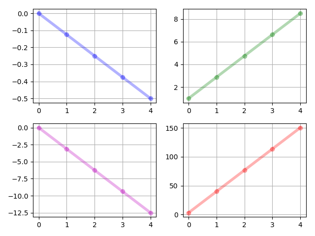
Figure 1: $\mathscr{X}(k)$ at time steps $k=0,1,2,3,4$ with cost function (22). The upper left figure shows $\mathbb{E}\left[x(k)\right]$. The upper right one shows $\mathbb{E}\left[x^{2}(k)\right]$. The lower left one shows $\mathbb{E}\left[x^{3}(k)\right]$ and the lower right one shows $\mathbb{E}\left[x^{4}(k)\right]$.

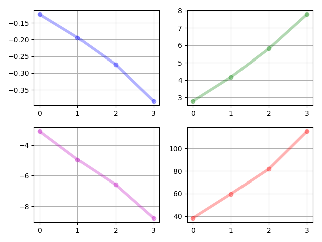
Figure 2: $\mathscr{U}(k)$ at time steps $k=0,1,2,3$ with cost function (22). The upper left figure shows $\mathbb{E}\left[u(k)\right]$. The upper right one shows $\mathbb{E}\left[u^{2}(k)\right]$. The lower left one shows $\mathbb{E}\left[u^{3}(k)\right]$ and the lower right one shows $\mathbb{E}\left[u^{4}(k)\right]$.

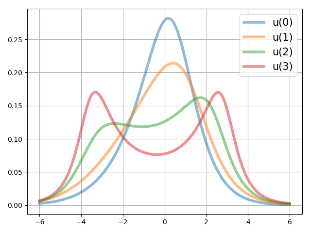
Figure 3: Realized control inputs $u(k)$ by $\mathscr{U}(k)$ for $k=0,1,2,3$ , which are obtained by cost function (22).

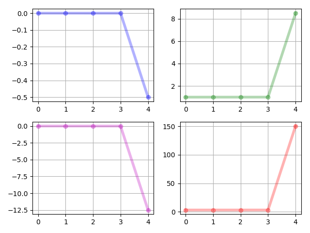
Figure 4: $\mathscr{X}(k)$ at time steps $k=0,1,2,3,4$ with cost function (23).

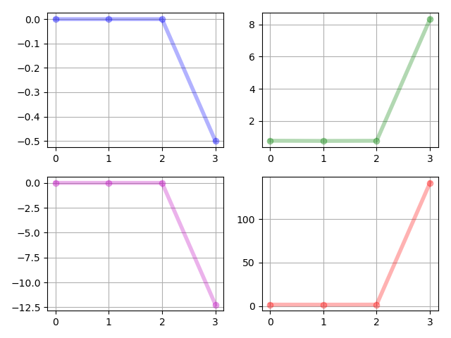
Figure 5: $\mathscr{U}(k)$ at time steps $k=0,1,2,3$ with cost function (23).

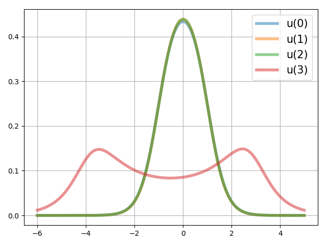
Figure 6: Realized control inputs $u(k)$ by $\mathscr{U}(k)$ for $k=0,1,2,3$, which are obtained by cost function (23).

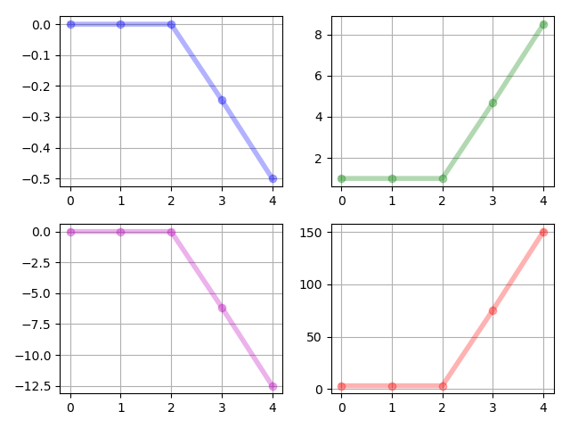
Figure 7: $\mathscr{X}(k)$ at time steps $k=0,1,2,3,4$ with cost function (32).

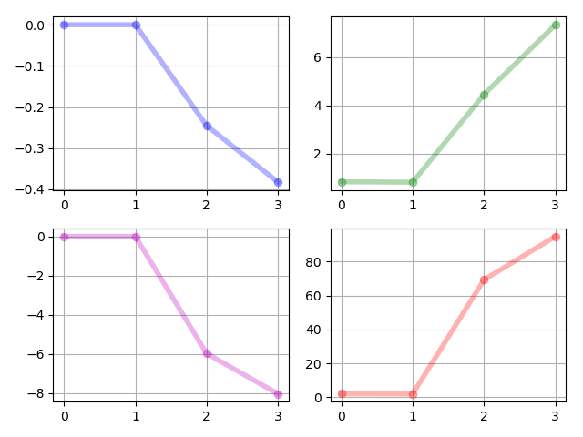
Figure 8: $\mathscr{U}(k)$ at time steps $k=0,1,2,3$ with cost function (32).

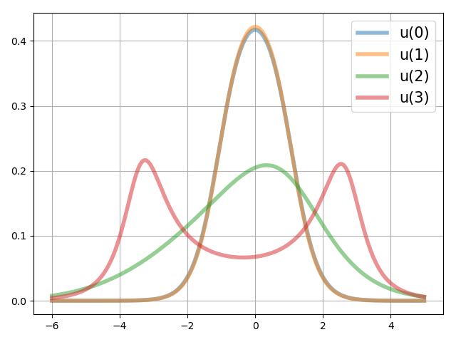
Figure 9: Realized control inputs $u(k)$ by $\mathscr{U}(k)$ for $k=0,1,2,3$, which are obtained by cost function (32).

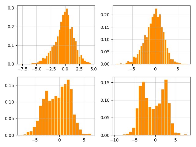
Figure 10: The histograms of $u_{i}(k)$ at time step $k$ for each agent $i$ by cost function (22). The upper left and right figures are $u_{i}(0)$ and $u_{i}(1),i=1,\cdots,1000$ respectively. The lower left and right figures are $u_{i}(2)$ and $u_{i}(3)$ respectively.

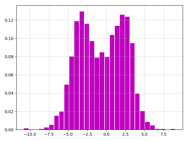
Figure 11: The histogram of the terminal system states $x_{i}(K)$ at time step $K=4$ for $i=1,\cdots,1000$ by cost function (22). It is close to the specified terminal distribution (31).

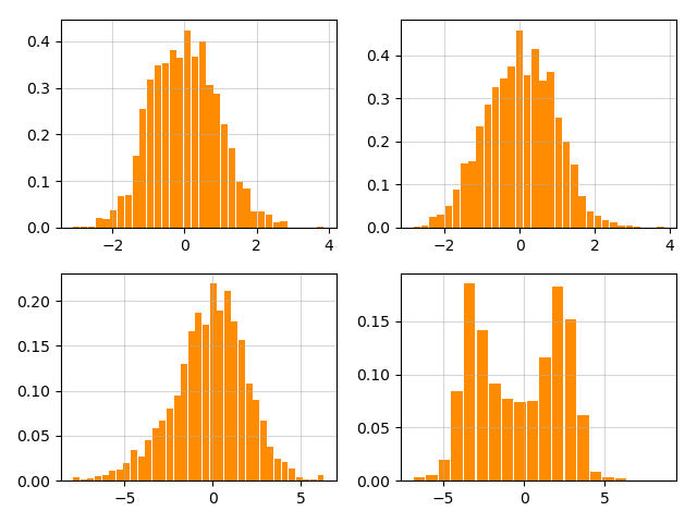
Figure 12: The histograms of $u_{i}(k)$ at time step $k$ for each agent $i$ by cost function (32).

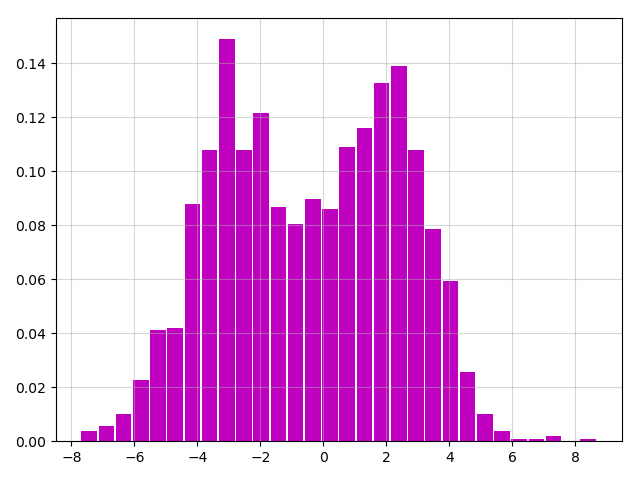
Figure 13: The histogram of the terminal system states $x_{i}(K)$ at time step $K=4$ for $i=1,\cdots,1000$ by cost function (32). It is close to the specified terminal distribution (31).

Then we treat the discrete distribution (occupation measure) steering problem defined in Problem 3.1 in [27]. The initial occupation measure $dq_{0}(x)$ composes of the i.i.d. samples drawn from the the continuous distribution $dq_{0}(x)$. Figure 10 shows the histograms of the $u_{i}(k)$ for each agent at time step $k=0,\cdots,3$, by cost function (22). Figure 11 shows the histogram of the terminal occupation measure of the agents. The two sharp peaks of the desired terminal state, of which the distribution is a mixture of two Laplacians, are well located at the desired points $x=-3$ and $x=2$. The histogram in 11 is very close to $q_{T}(x)$ in (31), which validates the performance of our proposed algorithm.

For the cost function of weighted energy effort and system energy (32), the histograms of the control inputs $u_{i}(k)$ are given in Figure 12. And the histogram of the terminal state of each agent $x_{i}(K)$ for $K=4$ is shown in Figure 13, where two sharp peaks are clearly located at $x=-3$ and $x=2$.

7.2 Two Laplacians to two Gaussians

Next, we consider the problem of steering the agents which are in separate groups to desired terminal groups. In this section, we simulate on steering a mixture of two Laplacians to a mixture of Gaussians. Both initial and terminal distributions have two modes. The initial one is chosen as

$$q_{0}(x)=\frac{0.5}{2}e^{|x-3|}+\frac{0.5}{2}e^{-|x+1|}.$$ (33)

and the terminal one is specified as

$$q_{T}(x)=\frac{0.5}{\sqrt{2\pi}}e^{\frac{(x-3)^{2}}{2}}+\frac{0.5}{\sqrt{2\pi}}e^{\frac{(x+3)^{2}}{2}}$$ (34)

The system parameters $a(k),k=0,\cdots,3$ are i.i.d. samples drawn from the uniform distribution $U[0.3,0.5]$. The dimension of each $\mathscr{U}(k)$ is $4$.

We first perform the control task with the cost function (22). The states of the moment system, i.e., $\mathscr{X}(k)$ for $k=0,1,2,3$ are given in Figure (14). The controls of the moment system, i.e., $\mathscr{U}(k)$ for $k=0,1,2,3$ are given in Figure (15). The realized controls in Figure (16) also show that the transition of the control inputs is smooth, even the task is to steer a distribution with two modes to another one with two modes. The results of discrete distribution (occupation measure) steering is given in Figure 20 and 21. The two modes of the histogram of the terminal states of the agents are well located at the desired points $x=\pm 3$.

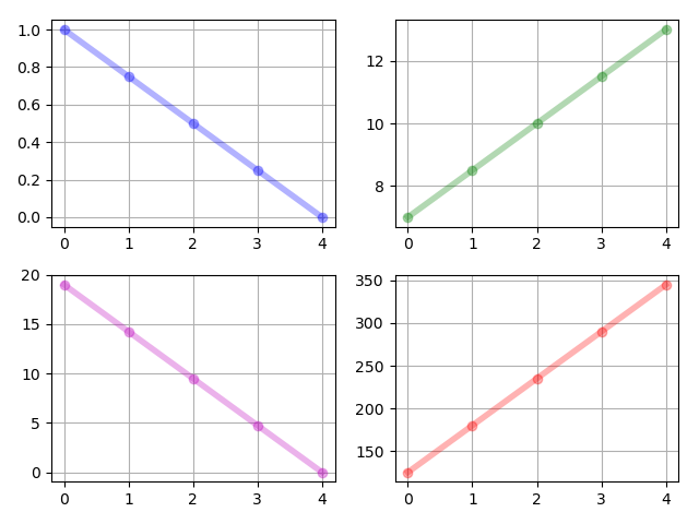
Figure 14: $\mathscr{X}(k)$ at time steps $k=0,1,2,3,4$ by cost function (22). The upper left figure shows $\mathbb{E}\left[x(k)\right]$. The upper right one shows $\mathbb{E}\left[x^{2}(k)\right]$. The lower left one shows $\mathbb{E}\left[x^{3}(k)\right]$ and the lower right one shows $\mathbb{E}\left[x^{4}(k)\right]$.

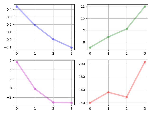
Figure 15: $\mathscr{U}(k)$ at time steps $k=0,1,2,3$ by cost function (22). The upper left figure shows $\mathbb{E}\left[u(k)\right]$. The upper right one shows $\mathbb{E}\left[u^{2}(k)\right]$. The lower left one shows $\mathbb{E}\left[u^{3}(k)\right]$ and the lower right one shows $\mathbb{E}\left[u^{4}(k)\right]$.

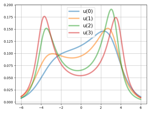
Figure 16: Realized control inputs $u(k)$ by $\mathscr{U}(k)$ for $k=0,1,2,3$, which are obtained by cost function (22).

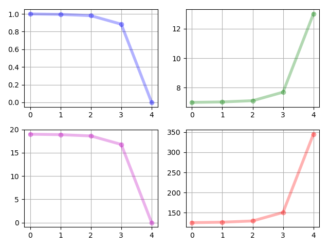
Figure 17: $\mathscr{X}(k)$ at time steps $k=0,1,2,3,4$ by cost function (32).

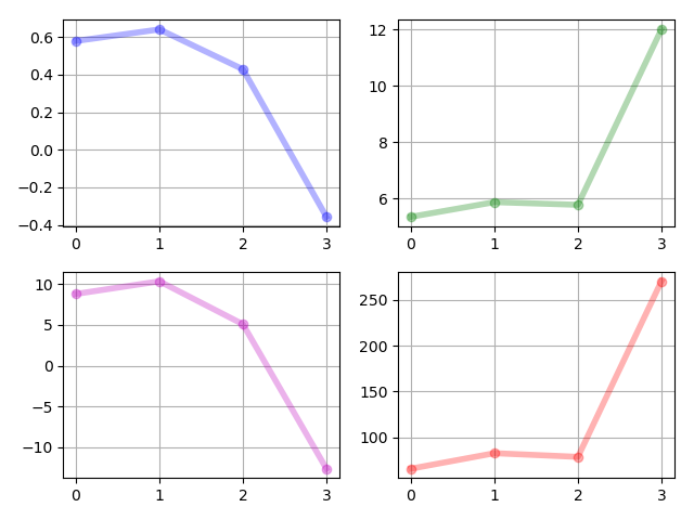
Figure 18: $\mathscr{U}(k)$ at time steps $k=0,1,2,3$ by cost function (32).

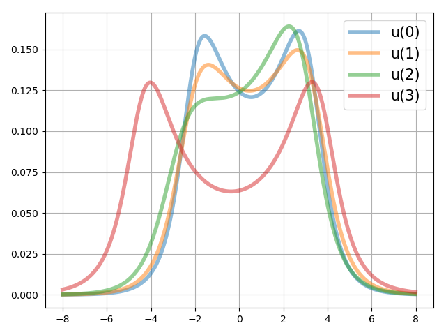
Figure 19: Realized control inputs $u(k)$ by $\mathscr{U}(k)$ for $k=0,1,2,3$, which are obtained by cost function (32).

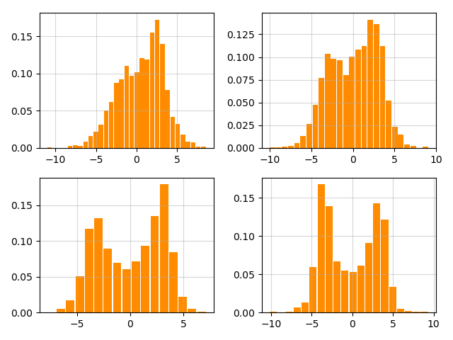
Figure 20: The histograms of $u_{i}(k)$ at time step $k$ for each agent $i$ by cost function (22). The upper left and right figures are $u_{i}(0)$ and $u_{i}(1),i=1,\cdots,1000$ respectively. The lower left and right figures are $u_{i}(2)$ and $u_{i}(3)$ respectively.

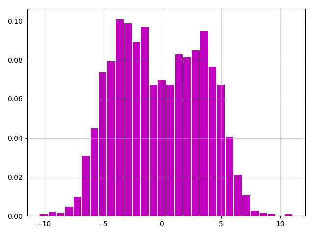
Figure 21: The histogram of the terminal system states $x_{i}(K)$ at time step $K=4$ for $i=1,\cdots,1000$ by cost function (22). It is close to the specified terminal distribution (34).

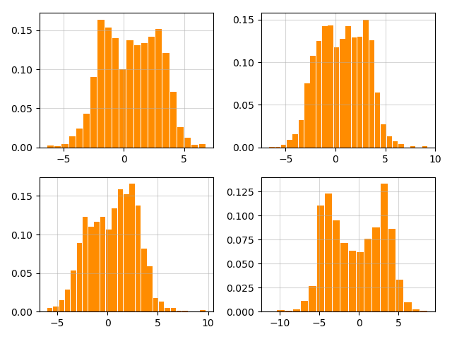
Figure 22: The histograms of $u_{i}(k)$ at time step $k$ for each agent $i$ by cost function (32).

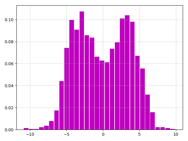
Figure 23: The histogram of the terminal system states $x_{i}(K)$ at time step $K=4$ for $i=1,\cdots,1000$ by cost function (32). It is close to the specified terminal distribution (34).

Next, we do optimization (21) with the cost function (24). In this simulation, we choose the cost function as (32). The simulation results are given in Figure 17, 18 and 19. The histogram of the terminal states of the agents is close to the desired continuous terminal distribution (34), which reveals the performance of our proposed algorithm.

8 A concluding remark

We consider the general distribution steering problem where the distributions to steer are arbitrary, which are only required to have first several orders of finite power moments. In our previous paper [26], we proposed a moment counterpart of the primal system for control. However, we was not able to put forward a control law based on optimization in the manner of conventional optimal control, which makes it hardly possible for us to obtain the control inputs by specific purposes, such as minimum energy effort. In this paper, we investigate the general distribution steering problem by convex optimization. The domain of the control inputs of the moment system is not convex and has a complex topology, which causes difficulty in optimization. We prove the controllability of the moment system and propose a set as the domain for optimization of which the convexity is proved. Then we consider different types of cost functions, including the smoothness of the state transition, the energy effort, the energy effort together with the system energy, and a general form of convex function, which is a weighted mixture of the energy effort and the system energy. A realization of the control inputs by the squared Hellinger distance is given to put forward a control scheme for the general distribution steering problem. We consider two typical scenarios in real application and formulate them as two distribution steering problems for simulation. The numerical results of the simulations validate our proposed algorithms. By the simulation results, we note that to yield smooth transition of the system states, one may need more energy.

In the future work, we would like to extend the results of this paper to nonlinear systems. System dynamics in the form of partial differential equations, such as Navier-Stokes equations, are of particular interest. We would also like to extend the results on the first-order system to more general systems, which will not be a trivial extension since the positive definiteness of the Hankel matrix will no longer be the sufficient and necessary condition for the existence of the multi-dimensional control inputs. Many results of this paper will not be valid any longer for the multi-dimensional systems and become difficult tasks.

In this appendix, we consider the approximation of $\frac{\partial\mathscr{U}(K-1)}{\partial\omega_{K-1}}$. By (3), we have

$$\mathbb{E}\left[x^{l}_{T}\right]$$ (35)

$$= \sum_{j=0}^{l}\binom{l}{j}a^{j}(K-1)\mathbb{E}\left[x^{j}(K-1)u^{l-j}(K-1)\right]$$

$$= \sum_{j=0}^{l}\binom{l}{j}a^{j}(K-1)\mathbb{E}\left[x^{j}(K-1)\right]\mathbb{E}\left[u^{l-j}(K-1)\right].$$

Then by (16), we have

$$\mathbb{E}\left[x^{l}_{T}\right]$$ (36)

$$= \sum_{j=0}^{l}\binom{l}{j}a^{j}(K-1)\left(\mathbb{E}\left[x^{j}(k_{0})\right]+\omega_{K-1}e_{j}\right)$$

$$\cdot \mathbb{E}\left[u^{l-j}(K-1)\right].$$

Let $e_{j}$ be the $j_{th}$ element of the vector $e(k_{0})$, i.e., $e_{j}=\mathbb{E}\left[x^{j}_{T}\right]-\mathbb{E}\left[x^{j}(k_{0})\right]$. Differentiate both sides of (35) over $\omega_{K-1}$ and we have

$$0= a^{l}(K-1)e_{l}$$ (37)

$$+ \sum_{j=1}^{l-1}\binom{l}{j}a^{j}(K-1)e_{j}\cdot\mathbb{E}\left[u^{l-j}(K-1)\right]$$

$$+ \sum_{j=1}^{l-1}\binom{l}{j}a^{j}(K-1)\left(\mathbb{E}\left[x^{j}(k_{0})\right]+\omega_{K-1}e_{j}\right)$$

$$\cdot \frac{\partial\mathbb{E}\left[u^{l-j}(K-1)\right]}{\partial\omega_{K-1}}+\frac{\partial\mathbb{E}\left[u^{l}(K-1)\right]}{\partial\omega_{K-1}}.$$

Since the absolute value of the second term of (37) is usually small, we have the following approximation

$$\frac{\partial\mathbb{E}\left[u^{l}(K-1)\right]}{\partial\omega_{K-1}}$$

$$\approx -a^{l}(K-1)e_{l}-\sum_{j=1}^{l-1}\binom{l}{j}a^{j}(K-1)e_{j}\cdot\mathbb{E}\left[u^{l-j}(K-1)\right],$$

for $l=1,\cdots,2n$. We can then write them as a matrix equation, which is

$$\frac{\partial\mathscr{U}(K-1)}{\partial\omega_{K-1}}\approx-\mathscr{A}(\mathscr{U}(K-1))e(k_{0}).$$

[]Guangyu Wu (S’22) received the B.E. degree from Northwestern Polytechnical University, Xi’an, China, in 2013, and two M.S. degrees, one in control science and engineering from Shanghai Jiao Tong University, Shanghai, China, in 2016, and the other in electrical engineering from the University of Notre Dame, South Bend, USA, in 2018.

He is currently pursuing the Ph.D. degree at Shanghai Jiao Tong University. His research interests are the moment problems and their applications to control theory and statistics.

[]Anders Lindquist (M’77–SM’86–F’89–LF’10) received the Ph.D. degree in optimization and systems theory from the Royal Institute of Technology, Stockholm, Sweden, in 1972, and an honorary doctorate (Doctor Scientiarum Honoris Causa) from Technion (Israel Institute of Technology) in 2010.

He is currently a Zhiyuan Chair Professor at Shanghai Jiao Tong University, China, and Professor Emeritus at the Royal Institute of Technology (KTH), Stockholm, Sweden. Before that he had a full academic career in the United States, after which he was appointed to the Chair of Optimization and Systems at KTH. Dr. Lindquist is a Member of the Royal Swedish Academy of Engineering Sciences, a Foreign Member of the Chinese Academy of Sciences, a Foreign Member of the Russian Academy of Natural Sciences, a Member of Academia Europaea (Academy of Europe), an Honorary Member the Hungarian Operations Research Society, a Fellow of SIAM, and a Fellow of IFAC. He received the 2003 George S. Axelby Outstanding Paper Award, the 2009 Reid Prize in Mathematics from SIAM, and the 2020 IEEE Control Systems Award, the IEEE field award in Systems and Control.

References

[1]
Shiba Biswal, Karthik Elamvazhuthi, and Spring Berman.
Decentralized control of multi-agent systems using local density
feedback.
IEEE Transactions on Automatic Control, 2021.
[2]
Christopher I Byrnes and Anders Lindquist.
A convex optimization approach to generalized moment problems.
In Control and modeling of complex systems, pages 3–21.
Springer, 2003.
[3]
Christopher I Byrnes and Anders Lindquist.
The generalized moment problem with complexity constraint.
Integral Equations and Operator Theory, 56(2):163–180, 2006.
[4]
Kenneth F Caluya and Abhishek Halder.
Reflected schrödinger bridge: Density control with path
constraints.
In 2021 American Control Conference (ACC), pages 1137–1142.
IEEE, 2021.
[5]
Yongxin Chen, Tryphon T Georgiou, and Michele Pavon.
Optimal steering of a linear stochastic system to a final probability
distribution, part i.
IEEE Transactions on Automatic Control, 61(5):1158–1169, 2015.
[6]
Yongxin Chen, Tryphon T Georgiou, and Michele Pavon.
Optimal steering of a linear stochastic system to a final probability
distribution, part ii.
IEEE Transactions on Automatic Control, 61(5):1170–1180, 2015.
[7]
Yongxin Chen, Tryphon T Georgiou, and Michele Pavon.
Optimal steering of a linear stochastic system to a final probability
distribution—part iii.
IEEE Transactions on Automatic Control, 63(9):3112–3118, 2018.
[8]
EG Collins and RE Skelton.
Covariance control discrete systems.
In 1985 24th IEEE Conference on Decision and Control, pages
542–547. IEEE, 1985.
[9]
EMMAN Collins and R Skelton.
A theory of state covariance assignment for discrete systems.
IEEE Transactions on Automatic Control, 32(1):35–41, 1987.
[10]
Karthik Elamvazhuthi, Matthias Kawski, Shiba Biswal, Vaibhav Deshmukh, and
Spring Berman.
Mean-field controllability and decentralized stabilization of markov
chains.
In 2017 IEEE 56th Annual Conference on Decision and Control
(CDC), pages 3131–3137. IEEE, 2017.
[11]
Tryphon T Georgiou and Anders Lindquist.
Kullback-leibler approximation of spectral density functions.
IEEE Transactions on Information Theory, 49(11):2910–2917,
2003.
[12]
Anthony Hotz and Robert E Skelton.
Covariance control theory.
International Journal of Control, 46(1):13–32, 1987.
[13]
Chen Hsieh and Robert E Skelton.
All covariance controllers for linear discrete-time systems.
IEEE transactions on automatic control, 35(8):908–915, 1990.
[14]
Ashkan Jasour, Allen Wang, and Brian C Williams.
Moment-based exact uncertainty propagation through nonlinear
stochastic autonomous systems.
arXiv preprint arXiv:2101.12490, 2021.
[15]
Ashkan M Jasour and Constantino Lagoa.
Reconstruction of support of a measure from its moments.
In 53rd IEEE Conference on Decision and Control, pages
1911–1916. IEEE, 2014.
[16]
Zhengyan Lin and Zhidong Bai.
Probability inequalities.
Springer Science & Business Media, 2011.
[17]
Fengjiao Liu, George Rapakoulias, and Panagiotis Tsiotras.
Optimal covariance steering for discrete-time linear stochastic
systems.
arXiv preprint arXiv:2211.00618, 2022.
[18]
Fengjiao Liu and Panagiotis Tsiotras.
Optimal covariance steering for continuous-time linear stochastic
systems with additive generic noise.
arXiv preprint arXiv:2206.11201, 2022.
[19]
Fengjiao Liu and Panagiotis Tsiotras.
Optimal covariance steering for continuous-time linear stochastic
systems with multiplicative noise.
arXiv preprint arXiv:2206.11735, 2022.
[20]
Kazuhide Okamoto, Maxim Goldshtein, and Panagiotis Tsiotras.
Optimal covariance control for stochastic systems under chance
constraints.
IEEE Control Systems Letters, 2(2):266–271, 2018.
[21]
Kazuhide Okamoto and Panagiotis Tsiotras.
Optimal stochastic vehicle path planning using covariance steering.
IEEE Robotics and Automation Letters, 4(3):2276–2281, 2019.
[22]
Augustinos D Saravanos, Isin M Balci, Efstathios Bakolas, and Evangelos A
Theodorou.
Distributed model predictive covariance steering.
arXiv preprint arXiv:2212.00398, 2022.
[23]
Carlo Sinigaglia, Andrea Manzoni, Francesco Braghin, and Spring Berman.
Robust optimal density control of robotic swarms.
arXiv preprint arXiv:2205.12592, 2022.
[24]
Vignesh Sivaramakrishnan, Joshua Pilipovsky, Meeko Oishi, and Panagiotis
Tsiotras.
Distribution steering for discrete-time linear systems with general
disturbances using characteristic functions.
In 2022 American Control Conference (ACC), pages 4183–4190.
IEEE, 2022.
[25]
Jan H van Schuppen.
Control and System Theory of Discrete-Time Stochastic Systems.
Springer, 2021.
[26]
Guangyu Wu and Anders Lindquist.
Density steering by power moments.
arXiv preprint arXiv:2211.02322, 2022.
[27]
Guangyu Wu and Anders Lindquist.
Group steering: Approaches based on power moments.
arXiv preprint arXiv:2211.13370, 2022.
[28]
Guangyu Wu and Anders Lindquist.
A non-classical parameterization for density estimation using sample
moments.
arXiv preprint arXiv:2201.04786, 2022.
[29]
Guangyu Wu and Anders Lindquist.
Non-gaussian bayesian filtering by density parametrization using
power moments.
arXiv preprint arXiv:2207.08519, 2022.
[30]
J-H Xu and Robert E Skelton.
An improved covariance assignment theory for discrete systems.
IEEE transactions on Automatic Control, 37(10):1588–1591,
1992.
[31]
Ji Yin, Zhiyuan Zhang, Evangelos Theodorou, and Panagiotis Tsiotras.
Trajectory distribution control for model predictive path integral
control using covariance steering.
In 2022 International Conference on Robotics and Automation
(ICRA), pages 1478–1484. IEEE, 2022.
[32]
Silun Zhang, Axel Ringh, Xiaoming Hu, and Johan Karlsson.
Modeling collective behaviors: A moment-based approach.
IEEE Transactions on Automatic Control, 66(1):33–48, 2020.
[33]
Tongjia Zheng, Qing Han, and Hai Lin.
Pde-based dynamic density estimation for large-scale agent systems.
IEEE Control Systems Letters, 5(2):541–546, 2020.
[34]
Tongjia Zheng, Qing Han, and Hai Lin.
Distributed mean-field density estimation for large-scale systems.
IEEE Transactions on Automatic Control, 2021.
[35]
Tongjia Zheng, Qing Han, and Hai Lin.
Transporting robotic swarms via mean-field feedback control.
IEEE Transactions on Automatic Control, 2021.
[36]
Albert Nikolaevič Širâev, Ralph Philip Boas, and Dmitrij Mihajlovič
Čibisov.
Probability-1.
Springer, 2016.