Modelling human logical reasoning process in dynamic environmental stress with cognitive agents

Abstract

Modelling human cognition can provide key insights into behavioral dynamics under changing conditions. This enables synthetic data generation and guides adaptive interventions for cognitive regulation. Challenges arise when environments are highly dynamic, obscuring stimulus-behavior relationships. We propose a cognitive agent integrating drift-diffusion with deep reinforcement learning to simulate granular stress effects on logical reasoning process. Leveraging a large dataset of 21,157 logical responses, we investigate performance impacts of dynamic stress. This prior knowledge informed model design and evaluation. Quantitatively, the framework improves cognition modelling by capturing both subject-specific and stimuli-specific behavioural differences. Qualitatively, it captures general trends in human logical reasoning under stress. Our approach is extensible to examining diverse environmental influences on cognition and behavior. Overall, this work demonstrates a powerful, data-driven methodology to simulate and understand the vagaries of human logical reasoning process in dynamic contexts.

Introduction

Understanding how humans make decisions under dynamic contexts is a fundamental challenge in modeling human cognition [1]. In particular, modeling the effects of environmental dynamics, such as stress [2] and feedback [3], on cognitive performance, could elucidate behavioral responses to tasks [2] and inform the design of feedback mechanisms to augment cognition [3]. Furthermore, such models may facilitate developing human-like robots [4, 5, 6] and enhancing human-agent collaboration [7, 8, 9]. Additionally, collecting and manually labeling human cognitive data poses substantial challenges. Computational models of cognition [10] enable generating synthetic datasets [11] and simulating environments for cognitive science research. These simulations could provide insights into the cognitive and neural functioning of biological systems [12], improving cognition modeling for applications including human decision prediction [13] and cognitive identity management [14].

The existing body of literature has amassed empirical evidence supporting the feasibility of modeling human cognition [15]. Traditional cognitive models, exemplified by BEAST [16] and the drift-diffusion model [17, 18], are characterized by closed-form structures. More recently, there has been a notable shift toward the integration of machine learning techniques [19] for simulating diverse human behaviors [20, 21, 22] across an array of tasks, including visual cognition [23, 24, 25], categorization [26, 27, 28, 29, 30], decision making [31, 32, 13, 33], game strategy [34], visual perception [35], word learning [36], probabilistic inference [37], point-and-click interactions [38, 39], and others. Of particular note, recurrent neural networks (RNNs) [1, 40, 41] have been adapted to execute various cognitive tasks [42] emulating human performance. RNNs have proven adept at simulating the intricate balance between accuracy and response time observed in biological vision [43].

However, prevailing research predominantly concentrates on modeling human cognition under standard and ideal conditions, often neglecting the nuanced impact of external stimuli [38, 39]. Alternatively, some studies treat external stimuli as a constant presence throughout the cognitive process [13]. We contend that a more nuanced modeling approach is imperative, particularly when dealing with dynamic stimuli that can fluctuate over time, contingent upon users’ performance. This nuanced approach involves stimuli variation at fine timescales, exerting a continuous influence on human cognitive behaviors. To illustrate, consider an animated visual stimulus conveying time pressure [44]. Such stimuli inform users of the passage of time, evoking sensations of pressure. Representing these stimuli as a binary existence indicator would oversimplify their nuanced effects. Therefore, our paper raises a fundamental question: How can we simulate the impact of dynamic environmental stimuli on the regulation of human cognitive behaviors with precision at a fine-grained level?

We aim to address this question by examining how dynamic time pressure stimuli [45], influences cognitive performance, particularly within the context of a math arithmetic task—a widely utilized benchmark for evaluating human cognition in logical reasoning [46, 47, 48]. The dynamism inherent in time pressure feedback encompasses two primary facets. Firstly, the presentation of time pressure can be dynamic, involving the delivery of progressively changing visual frames over time (Fig. 2(a)), thereby instilling a sense of urgency. Secondly, the presence of time pressure may vary dynamically across different trials. Existing research has underscored the impact of time pressure on human cognition and productivity [49]. Temporal cues have been shown to enhance focus [50] and arousal [51]. However, heightened time pressure may lead to an excessive mental workload, resulting in deteriorated response quality [2]. A recent study in the domain of visuomotor tasks [44] demonstrated that time pressure could reduce response time while concurrently increasing behavioral errors. In sum, time pressure stimuli represent a well-established feedback modality capable of modulating human cognitive performance. The modeling of cognition performance under dynamic time pressure holds the promise of offering valuable insights into cognitive behaviors and facilitating the development of adaptive intervention mechanisms for regulating user performance.

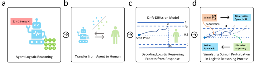
Figure 1: Illustration of the overall framework. First, we train a logical reasoning agent to solve cognitive tasks without considering users’ response. Second, we transfer features extracted from the logical reasoning agent without time pressure to real user choice and response time (initial estimation). Third, the initial estimated response time and predicted choice probability generate evidence accumulation trajectory in the drift-diffusion model. Lastly, the DRL agent simulates influence of stimuli perturbation on cognitive process by taking dynamic environmental stimuli as input and take specific action to modulate evidence accumulation process. When evidence accumulator achieves boundary threshold, the final prediction of response time is generated and DRL agent achieves terminate state.

In this paper, we introduce a systematic hybrid framework with deep reinforcement learning (DRL) depicted in Fig. 1. This framework integrates a classical closed-form cognitive model into a data-driven DRL approach, allowing for the comprehensive modeling of the impacts of dynamic, fine-grained time pressure stimuli. While neural networks (NNs) are recognized for their proficiency in function approximation and have been applied to model cognitive behaviors [13], their inherent black-box nature poses challenges in representing the internal mechanisms of the cognitive process. Consequently, utilizing a NN directly to simulate the dynamic effects of stimuli on cognition in a fine-grained manner becomes challenging. Recent efforts such as task-DyVA [1] focus on modelling cognitive response time in task-switching games instead of how human cognition responds to external stimuli. To address this limitation, our framework integrates DRL with the drift-diffusion model (DDM), a sequential sampling method widely employed in cognitive modeling [17, 18]. DDM posits that humans make decisions by accumulating evidence until a boundary threshold is reached [52]. The simulated choice and response time are then determined based on the corresponding boundary and accumulation time. While DDM excels in representing the cognition process in an explicable and fine-grained manner, it primarily focuses on posterior estimation of user decisions rather than predicting users’ future performance under stimuli. On the other hand, DRL, with NN at its core, offers a step-by-step interaction environment. This environment enables the incorporation of the fine-grained cognition process inherent in DDM while retaining the function approximation capabilities of NN. This hybrid approach bridges the gap between the transparency of classical cognitive models and the flexibility of data-driven methods, presenting a promising avenue for modeling the intricate dynamics of cognition under dynamic time pressure stimuli.

Our framework employs the DRL agent to encapsulate the modulation of the evidence accumulation (EA) process within the drift-diffusion model (DDM) induced by time pressure stimuli. In a detailed breakdown, the time pressure visual stimuli are discretized into frames corresponding to the steps in the EA process. At each step, the DRL agent takes the corresponding time pressure visual stimuli as input and introduces a positive, neutral, or negative bias in the EA process. This bias alters the EA, resulting in an earlier or later achievement of the boundary threshold. This, in turn, signifies a faster or slower response compared to cases without the stimuli. This hybrid modeling approach, specifically the integration of DRL to simulate external stimuli within the DDM in a fine-grained manner considering subject-specific and stimuli-specific behavioural differences, distinguishes our framework from previous works that primarily focus on modeling coarse-grained posterior estimation of decision and response time using reinforcement learning [53, 54]. Subsequently, we delve into the intricacies of the model architecture and modelling results.

Results

Hybrid cognitive agent framework

Our framework comprises four key steps, as illustrated in Fig. 1. In the initial step, we train a recurrent neural network (RNN)-based logical reasoning agent to proficiently solve the designated cognitive task. Following this, the second step involves the knowledge transfer from these trained agents to establish mappings from the RNN agent to human performance metrics. This results in human response time and accuracy for each trial. Moving to the third step, we employ a fine-grained Drift-Diffusion Model (DDM) to decode human performance, extracting detailed information about response time and accuracy. This step is pivotal in generating the evidence accumulation process (EA) reflective of the underlying cognitive mechanisms. In the final step, we introduce a deep reinforcement learning (DRL) agent to the framework. This agent plays a crucial role in simulating the impact of stimuli perturbation on the evidence accumulation process. By leveraging DRL, we can capture the nuanced dynamics of how external stimuli, such as time pressure, influence the intricate logical reasoning processes modeled by the DDM. This multi-step approach allows us to bridge the gap between logical reasoning agents, human performance, and the fine-grained representation of logical reasoning processes under dynamic stimuli.

To simulate the impact of dynamic time pressure, it is imperative to initially predict users’ baseline performance in the absence of time pressure. Drawing inspiration from prior research that models human subjects’ time perception by capturing internal activities in perceptual classification networks [55], we have devised a baseline prediction model. Specifically, Roseboom et al. [55] constructed a neural network functionally akin to human visual processing for image classification. The network was then exposed to input videos of natural scenes, causing changes in network activation. The accumulation of salient changes in activation was subsequently utilized to estimate duration, effectively gauging the perceived passage of time in the video through a Support Vector Machine (SVM).

Similarly, our baseline prediction model employs a long short-term memory (LSTM) neural network to address cognitive tasks [42]. In particular, we train an LSTM-based math answer agent (Fig. 1(a)) to learn and respond to math questions, thereby achieving functional similarity with human cognition in math tasks. The intermediate output of the LSTM layer serves as input features for an SVM, establishing mappings between agents and humans to estimate user choice and response time (Fig. 1(b)). The rationale underlying this approach is rooted in the recognition that distinct math questions may pose varying levels of difficulty, leading to user choice biases and variations in response time. The LSTM-based agent has the capacity to capture these potential differences in difficulty levels, and the SVM is employed to map these to user choice and response time, offering a comprehensive prediction of baseline performance.

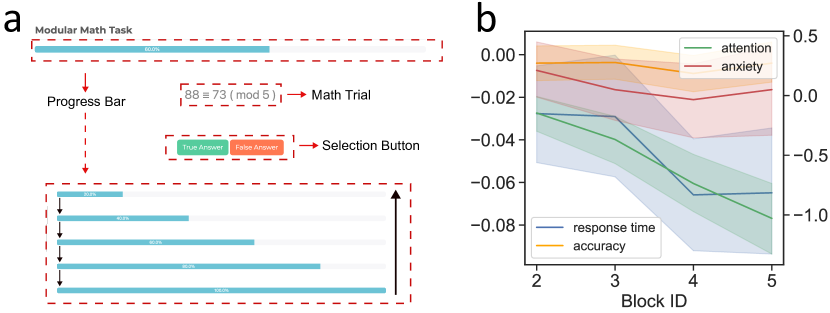
Figure 2: a: Math arithmetic task. Each math trial is composed of two two-digit numbers $Num_{1},Num_{2}$ and one one-digit numer $Num_{3}$, formatted as: $Num_{1}\equiv Num_{2}\,(\,mod\,Num_{3})$. To solve this question, participants first use $Num_{1}$ to subtract $Num_{2}$ and judge whether the subtraction result could be divisible by $Num_{3}$. If it is divisible, they select "True" button. Otherwise, they select "False" button. When the time pressure feedback happens, a progress bar will be shown on top of the math question, which adds one unit for each second and reset and add again when it accumulates five units. b: Overall trend of relative change of response time/accuracy (left y axis), and attention/anxiety (right y axis), respectively, across 4 blocks.

To simulate how dynamic time pressure affects user performance, we conceptualize the logical reasoning process as an evidence accumulation (EA) process in line with the Drift-Diffusion Model (DDM) [17] (Fig. 1(c)). The EA process enables the segmentation of users’ cognition into sequential steps, facilitating the fine-grained modeling of dynamic time pressure. The boundary threshold and accumulation time parameters in the DDM are derived from the predicted responses obtained from the previous SVM model.

In order to simulate the dynamic impact of time pressure visual stimuli, we introduce a Deep Reinforcement Learning (DRL) agent. The visual stimuli are segmented into frames, aligning with the steps in the EA process. For each frame, the specific visual stimuli are applied to the DRL agent (Fig. 1(d)), which, akin to how participants’ logical reasoning processes may be influenced by each frame of stimuli, modulates the EA process.

In particular, for each frame of time pressure stimuli, the DRL agent adjusts the EA process by introducing positive, neutral, or negative bias (action space of the DRL agent). This modulation may result in the evidence accumulator reaching the boundary threshold either earlier or later. The output from this DRL-modulated EA process serves as the final prediction for user response time. Additional details regarding the design and implementation of this framework are presented in Methods section.

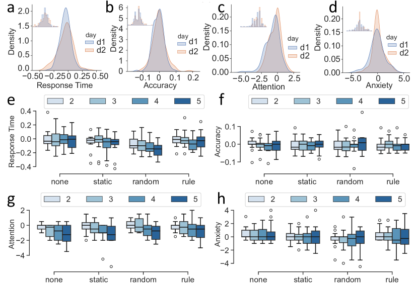
Figure 3: a,b,c,d: overall distribution of relative change of response time (a), accuracy (b), attention (c), and anxiety (d), respectively, across 2 days. e,f,g,h: box plot of relative change of response time (e), accuracy (f), attention (g), and anxiety (h), respectively, across 4 groups and 4 blocks.

Dataset collection and exploration

We have compiled an extensive dataset encompassing 21,157 logical responses from 50 participants engaged in math modular tasks, as outlined in Fig. 2(a). To enhance the diversity of the dataset and evaluate the cognition model under dynamic environmental stress, participants were randomly and uniformly distributed across four distinct groups: None Group: Participants experienced no time pressure for any trial. Static Group: Time pressure was consistently applied for each trial. Random Group: There was a 50% probability of time pressure being applied for each trial. Rule Group: Time pressure was adaptively applied based on users’ past performance. Each participant engaged in a two-day study, featuring one exercise session (20 trials) and one formal session (300 trials) per day. During the formal session, participants provided their choice and response time for each trial. Additionally, participants were requested to rate their current attention/anxiety status on a 7-point Likert scale every 30 trials. The final dataset comprises approximately 21,157 samples (trials), capturing a diverse range of cognitive responses under varying time pressure conditions.

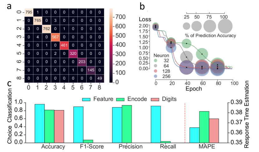
Figure 4: a. Confusion matrix (x axis: ground truth, y axis: prediction) for testing set prediction of the logical reasoning agent (LSTM neuron = 256). b. Training loss and accuracy with training epochs across four kinds of LSTM neurons of the logical reasoning agent. c. Performance of user choice classification of SVC models and response time estimation of SVR models across three math question representations: Feature label: SVM takes features extracted from logical reasoning agent as input, Encode label: SVM takes encoded vectors of raw math numbers as input, Digits label: SVM takes raw math numbers as input.

To comprehensively investigate the impact of different time pressure stimuli on cognition performance, we conducted an initial exploratory analysis on the dataset. To mitigate the influence of chance factors, we divided the 300 trials of the formal session into five blocks of equal size and calculated the block-wise averages for accuracy, response time, attention, and anxiety scores. Recognizing the inherent variability in users’ baseline performance, we aimed to elucidate the impact of time pressure across different groups by comparing the relative change in user performance and status across the four groups. Specifically, let $R_{i}$ denote the average result of $Block_{i}$, where $R_{1}$ ($Block_{1}$) represents the baseline performance. The final relative result for $Block_{i}$ ($i>1$) is $(R_{i}-R_{1})/R_{1}$ for accuracy and response time change and $R_{i}-R_{1}$ for attention and anxiety change. This adjustment accounts for the fact that attention/anxiety scores linearly reflect user status, while response time/accuracy changes need to be normalized against participants’ individual baseline performances. The obtained results underwent analysis using repeated-measures ANOVA. To discern specific differences, Bonferroni-corrected paired post hoc t-tests were employed for pairwise comparisons between the groups, enabling a thorough exploration of the impact of different time pressure stimuli on cognition performance and user status.

Response time

In the analysis of between-subjects effects, the ANOVA revealed a significant effect of Group ($F_{3,32}=3.015,P=0.044<0.05$) (Fig. 3(e)). Specifically, a significant difference was identified between the none group (mean $\pm$ SD: $-0.012\pm 0.021$) and the random group ($-0.105\pm 0.025$) with $p=0.039<0.05$. The rule group showed a larger reduction in response time ($-0.034\pm 0.021$) compared to the none group but a smaller reduction compared to the static group ($-0.054\pm 0.022$). Notably, the random group exhibited the most substantial reduction in response time. These results suggest that different types of time pressure stimuli may exert varying effects on response time.

Regarding within-subjects tests, a significant effect was observed across blocks ($F_{3,96}=7.121,P<0.001$) (Fig. 3(e)), specifically between the following blocks: $Block_{2}$ ($-0.031\pm 0.011$) vs. $Block_{4}$ ($-0.070\pm 0.014$): $p=0.023<0.05$, $Block_{2}$ vs. $Block_{5}$ ($-0.072\pm 0.014$): $p=0.026<0.05$, $Block_{3}$ ($-0.033\pm 0.013$) vs. $Block_{4}$: $p=0.008<0.01$, $Block_{3}$ vs. $Block_{5}$: $p=0.025<0.05$.

No interaction was found between Block and Group ($F_{9,96}=0.958,P=0.48$). Furthermore, there was no significant effect of Date ($F_{1,32}=0.003,P=0.959$) (Fig. 3(a)), and no other significant interaction effects were identified (all $P>0.05$). These findings provide valuable insights into the differential impact of time pressure stimuli on response time and underscore the significance of within-subject variations across different blocks.

Accuracy

No significant effect was observed in Group ($F_{3,32}=0.081,P=0.97>0.05$), Block ($F_{3,30}=0.313,P=0.816>0.05$) (Fig. 3(f)), or Date ($F_{1,32}=0.861,P=0.36>0.05$) (Fig. 3(b)). Additionally, no other significant interaction effects were identified (all $P>0.05$). This outcome aligns with expectations, as participants were instructed to prioritize accuracy over response time consistently. Consequently, the accuracy of users’ choices should generally be high, while response time may vary depending on the stimuli. The lack of significant effects in these factors supports the experimental design and participants’ adherence to the specified priority in their decision-making process.

Attention

No significant effect was detected in Group ($F_{3,32}=0.532,P=0.664>0.05$) (Fig. 3(g)). However, a significant effect emerged in Block ($F_{3,96}=27.366,P<0.001$) (Fig. 3(g)) and Date ($F_{1,32}=8.693,P=0.006<0.01$) (Fig. 3(c)). An interaction was also identified between Block and Date ($F_{3,96}=9.012,P<0.001$). Notably, no other significant interaction effects were observed (all $P>0.05$).

Anxiety

No significant effect was observed in Group ($F_{3,32}=0.925,P=0.44>0.05$) and Block ($F_{3,30}=1.243,P=0.312>0.05$) (Fig. 3(h)). However, a significant effect was found in Date ($F_{1,32}=4.165,P=0.05$) (Fig. 3(d)). Interactions were identified between Block and Date ($F_{3,30}=3.737,P=0.022<0.05$) and Date and Group ($F_{3,32}=5.458,P=0.004<0.01$). No other significant interaction effects were found (all $P>0.05$).

The results presented above suggest that both time pressure stimuli and block number may impact users’ response time. This evidence contributes valuable insights and aligns with prior knowledge, providing a foundation to inform the design of our cognition model. The observed effects underscore the relevance of considering these factors in modeling and understanding the dynamics of user response time under varying conditions.

Logical reasoning agent to solve math questions

We hypothesize that participants’ varied responses to different math questions stem from features inherent in the questions, such as difficulty levels. These features may influence user choice and response time even in ideal conditions (i.e., without external stimuli). To capture such features, we initially train a logical reasoning agent capable of solving math questions in a manner similar to humans. Subsequently, feature representations are extracted from the intermediate output of this logical reasoning agent.

Illustrated in Fig. 1, we employ an LSTM-based logical reasoning agent (architecture details in Methods section) that takes a math question as input and outputs the corresponding answer. For example, given the sequence "61 $\equiv$ 26(mod 4)" as input, the agent outputs "3" (the remainder of the subtraction result, "35," of "61" and "26," divided by "4"). It is essential to note the distinction from the data collection process, where users are required to choose whether the subtraction result ("35") of "61" and "26" is divisible by "4"—a binary selection task.

In other words, the logical reasoning agent is trained to answer math arithmetic tasks correctly, rather than to predict user responses. This design choice ensures that the agent learns the potential arithmetic reasoning process and generates representative features of math questions, rather than performing a binary classification task.

We curated an independent dataset (Methods section) specifically designated for training (80%) and testing (20%) the logical reasoning agent. Given that the first two numbers of math questions are both two-digits, the arithmetic reasoning result is chosen from 0 to 8. Consequently, the ground truth encompasses 9 classes. To optimize performance, we experimented with different numbers of output neurons (32, 64, 128, 256) from the LSTM layer.

After 100 epochs of training, the logical reasoning agent with 256 neurons achieved remarkable results, attaining a training loss of 0.0001 and 100% accuracy (Fig.4(b)). The confusion matrix (Fig.4(a)) for the testing set demonstrates that this neuron configuration yields over 99% accuracy for all classes, resulting in an overall test accuracy of 99.93%. These outcomes affirm that the LSTM-based logical reasoning agent adeptly solves math arithmetic problems in the majority of cases. This aligns with existing work [56, 57], which has demonstrated the capacity of neural networks to learn mathematical equivalence. The success of the logical reasoning agent in solving arithmetic problems lays a foundation for extracting representative features from math questions to construct cognition models.

Transfer from agents to humans

As previously mentioned, the second step in our simulation framework (Fig. 1) involves transferring features captured by the logical agent to real responses of humans by utilizing SVM models to predict users’ baseline performance without time pressure. The features comprise the intermediate output of the LSTM layer, with the output neuron number set to 256, resulting in 256 features captured by the math answer agent. During cognition performance analysis, we observed that users’ performance is influenced by the block number. Therefore, for each trial, we introduce the question id as an additional input feature, concatenated with the previous 256 features for SVM models. The question id denotes the corresponding trial number in the dataset, resulting in a total of 257 features for predicting user response for each sample/trial. Users’ response encompasses both user choice and response time. Consequently, the SVM models consist of a binary SVM classifier (SVC) to predict user choice (True or False selection) and an SVM regressor (SVR) to estimate users’ response time.

To evaluate the SVC model, we use accuracy, precision, recall, and F1-score metrics. For the SVR model, we employ Mean Average Percentage Error (MAPE) for evaluation. To demonstrate that the math answer agent has indeed captured useful and representative features from the math questions, we compare the SVM models with two additional settings where the SVM models do not take features captured from the math answer agent as input. Instead, they take raw three-digit numbers from the math questions or encoded vectors (Methods section) of raw numbers as input, along with the question id. The SVM performance in the three settings is depicted in Fig.4(c). Notably, SVM models with features from the math answer agent exhibit significantly higher accuracy (0.9613) and F1-score (0.8996) for user choice prediction and lower MAPE (0.3652) for response time estimation than the other two settings. These results underscore the effectiveness of the math answer agent in capturing representative features from math questions and the feasibility of predicting user baseline performance with the SVM models.

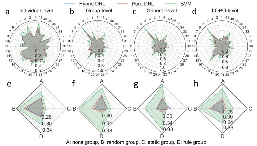
Figure 5: a,b,c,d,e,f,g,h: Average MAPE for each participant (a,b,c,d)/group (e,f,g,h) in predictions of testing set from Hybrid DRL agent, Pure DRL agent, and SVM model in four training strategies (a,e. Individual-Level, b,f. Group-Level, c,g. General-Level, d,h. LOPO-Level), respectively. (The number around the circle represents participant id in a,b,c,d).

Simulating time pressure stimuli perturbation on user performance with the hybrid DRL agent

Having obtained users’ baseline performance from SVM models, the subsequent step involves modeling the effect of time pressure on user performance. Since users’ accuracy is minimally affected by such stimuli, as indicated by the user study mentioned earlier, our focus shifts to estimating users’ response time. To showcase the merit of the hybrid DRL design, we introduce a baseline DRL model termed the "Pure DRL agent", which does not incorporate the Drift-Diffusion Model (DDM). Specifically, this Pure DRL agent does not segment time pressure visual stimuli into frames. Instead, for each trial from the dataset, if the time pressure stimuli exist, it directly takes the entire visual stimuli as input and outputs one action representing the overall change in response time due to time pressure. The final estimation of regulated response time is the sum of this action and the basic response time estimated by SVR models (further details are provided in Methods section). We conduct a comparative analysis between the hybrid and pure DRL agent designs across three key aspects: response time estimation performance, agent training efficiency, and interpretability. This comparison aims to highlight the advantages and effectiveness of the hybrid DRL approach in capturing the nuanced dynamics of time pressure stimuli on user response time.

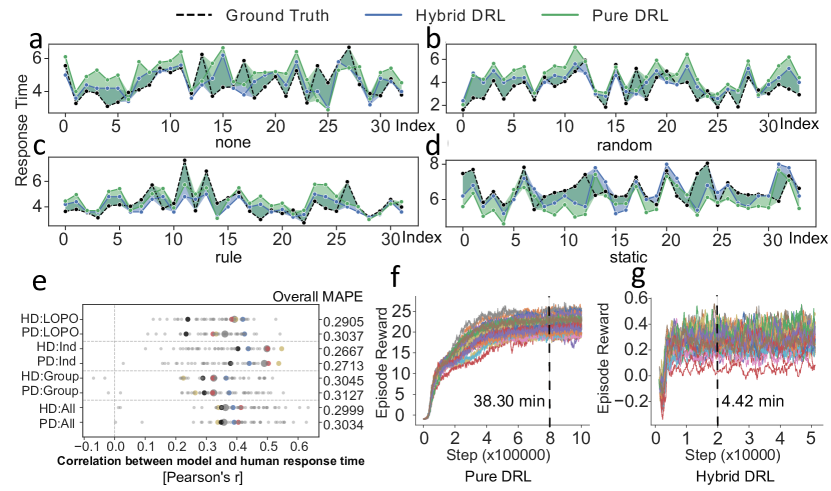
Figure 6: a,b,c,d: Examples of user response time in chronological order from one participant in each group predicted from Hybrid/ Pure DRL agent in LOPO-level training, compared with ground truth. e: Pearson correlation between predictions from Hybrid/ Pure DRL agent (HD: Hybrid DRL, PD: Pure DRL) and human real response time (ground truth) in four training strategies (All: General-level, Group: Group-level, Ind: Individual-level, LOPO: LOPO-level). Small gray dots, medium dots, and large gray dots represent Pearson correlation of prediction results from each participant’s testing set, each group’s testing set (red:none, yellow:static, black:random, blue:rule) and whole testing set, respectively. The right y axis depicts overall average MAPE of two agents in four training strategies. f,g: Training curve for Pure DRL (f) and Hybrid DRL (g) model.

Response time simulation

We employ both Mean Average Percentage Error (MAPE) and Pearson correlation to compare the performance of the hybrid DRL and Pure DRL agents. Four model training strategies are used for comparison: general-level, group-level, individual-level, and Leave-One-Participant-Out (LOPO)-level. General-level involves splitting the entire dataset into training (80%) and testing (20%) sets for overall model evaluation. Group-level trains and tests a specific model using data from each group, revealing performance across different time pressure stimuli. Individual-level trains and tests a model using data from a specific participant, assessing personalized model feasibility incorporating subject-specific behavioural differences. Shuffling is applied to the training and testing sets to prevent overfitting artifacts. As shuffled testing disrupts the temporal trend of user response time aross different math trials, we incorporate LOPO-level as an additional training strategy. This strategy selects all data from one participant as the testing set and uses data from other participants in the same group as the training set. By traversing every participant’s data as the testing set, we ensure a comprehensive assessment of the model’s performance in capturing the temporal trend of response time.

Fig. 5 illustrates the average Mean Average Percentage Error (MAPE) of the testing set for each individual user (a,b,c,d) and each group (e,f,g,h) using both the hybrid DRL and Pure DRL agents in the four training strategies. The baseline prediction results of SVM models without time pressure stimuli simulation are also presented. Both the hybrid DRL and Pure DRL agents show improvement in response time estimation compared to SVM results. However, the hybrid DRL agent consistently achieves lower MAPE compared to the Pure DRL agent in most cases, indicating the superiority of the hybrid DRL agent in response time estimation.

The overall average MAPE for the entire testing set by both agents is depicted on the right y-axis of Fig. 6(e), further supporting this conclusion. Fig. 6(e) also reveals that the hybrid DRL agent exhibits larger Pearson correlation in individual testing sets (small dots), group testing sets (medium dots), and the whole testing set (large dots) compared to the Pure DRL agent in most cases, across all four training strategies. Both MAPE and Pearson correlation demonstrate the superior performance of the hybrid DRL agent in modeling the effect of time pressure stimuli.

To compare which agent design better captures the trend of response time change in users’ overall tasks, we visualize prediction results and real user response time for the testing set from one participant of each group in LOPO-level in chronological order (Fig. 6(a,b,c,d)). The predicted and real response time curves clearly demonstrate that the hybrid DRL agent more accurately captures the trend of user response time compared to the Pure DRL agent.

Training efficiency

The training curves for both agents are presented in Fig. 6(f,g). The Pure DRL and hybrid DRL agents converge at approximately 800,000 steps and 20,000 steps, respectively. It’s important to note that the meanings of one step differ between the two agents. For the hybrid DRL agent, one step represents one frame of time pressure stimuli during one trial, whereas one step for the Pure DRL agent represents the entire trial. Consequently, a direct comparison of steps is not meaningful. Instead, we compare the training time required for both agents to achieve convergence on the same hardware (GeForce RTX 2080 Ti) and the same dataset. The results in Fig. 6(f,g) indicate that the hybrid DRL agent converges in approximately 1/10 of the time compared to the Pure DRL agent (4.42 minutes vs. 38.30 minutes). This outcome underscores the advantage of incorporating an explicit cognitive model (i.e., the DDM) in the hybrid DRL agent.

Interpretability

An essential advantage of the cognition-inspired hybrid DRL agent is its interpretability. The Pure DRL agent directly outputs estimated response time changes for each trial, obscuring the internal mechanism regarding how time pressure stimuli modulate the logical reasoning process. In contrast, the hybrid DRL agent can generate a trajectory of the time pressure effect on response time corresponding to the users’ logical reasoning process. Therefore, visualizing the trajectories of the hybrid DRL agent enables the extraction of new insights into how time pressure stimuli affect the human logical reasoning process.

We explore this benefit in Fig. 7(a,b,c,d,e,f,g,h). Here, the action trajectory represents the trajectory of actions taken by the hybrid DRL agent during one episode, with each episode corresponding to one math trial of users. The time pressure effect trajectory is the accumulated actions multiplied by $\delta_{p}$. $\delta_{p}$ represents one unit of evidence per step, transforming the normalized action value into the evidence accumulation process. We visualize the time pressure effect trajectories across the four groups in Fig. 7(a,b,c,d). Each curve represents one trajectory predicted by the hybrid DRL agent during one trial.

We observe that the time pressure effect trajectories are more concentrated in the random and rule groups but divergent in the none and static groups (Fig. 7(a,b,c,d)). This suggests that participants in the random and rule groups, especially the random group, are better regulated by the corresponding type of time pressure stimuli, resulting in similar trends in all time pressure effect trajectories in this group. Quantitatively, the random group has the lowest standard deviation (STD) of action trajectories (Fig. 7(g)) and the highest average value and slope for the time pressure effect trajectories (Fig. 7(f,h)). These findings indicate that the random group experiences the most effective regulation of user cognition performance.

This observation aligns with the expectation that users may quickly adapt to none time pressure or static time pressure, ceasing to be regulated by them after a few trials. However, users may not anticipate the time pressure stimuli in the random group, leading to a more prolonged regulation effect.

This result is also consistent with the earlier user study findings (Fig. 3(e)), where participants in the random group demonstrated a significantly larger reduction in response time. These experiments affirm the hybrid DRL agent’s capability to explain and support the observations in the user study.

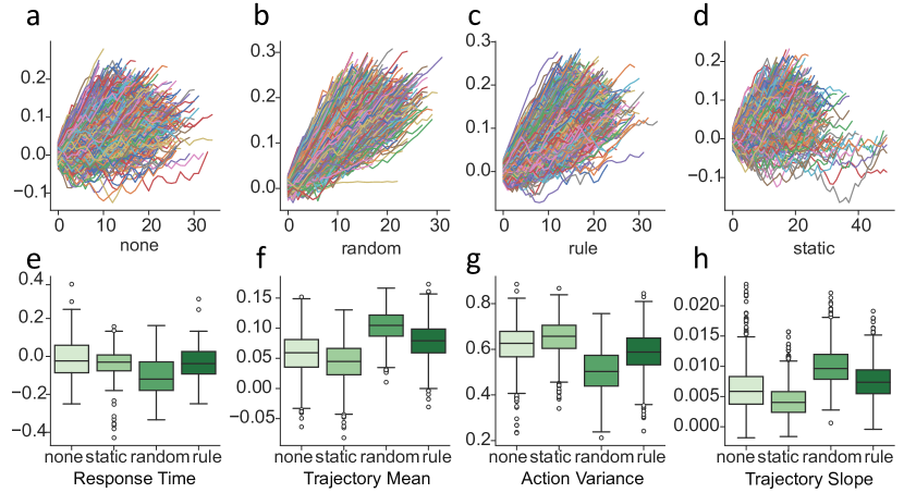
Figure 7: a,b,c,d: Time pressure effect trajectories of four groups, respectively. e: Box plot of relative response time change across four groups in the whole dataset. f,g,h: Box plot of mean value of time pressure effect trajectories (f), standard deviation of action trajectories (g), slope of time pressure effect trajectories (h) of four groups in predicted testing dataset by Hybrid DRL agent. The slope of one trajectory is calculated from the start point to the end point of the trajectory.

Discussion

Cognition modeling is a fundamental aspect of understanding human cognitive behaviors [1]. Traditional cognitive models such as BEAST [16] and the drift-diffusion model [17, 18] have provided insights, while machine learning techniques [19] offer a data-driven approach to modeling cognitive processes [1, 20, 21, 22, 23, 24, 25, 26, 27, 28, 29, 30, 31, 32, 13, 33]. However, machine learning techniques often face challenges related to interpretability due to their black-box nature. To address this limitation, we introduce an explainable cognition model, the drift-diffusion model, into the cognitive process. By combining this model with machine learning techniques, we create an interpretable framework to simulate the impact of environmental dynamics on the cognitive process. This integration enhances our ability to understand and interpret the complex interactions between environmental stimuli and cognitive behaviors.

Current research predominantly focuses on modeling human cognition under standard and ideal conditions, often overlooking the nuanced impact of external stimuli [38, 39]. Alternatively, some studies treat external stimuli as a constant presence throughout the cognitive process [13]. We argue that a more nuanced modeling approach is imperative, especially when dealing with dynamic environmental stimuli that can fluctuate over time based on users’ performance. This nuanced approach involves stimuli variation at fine timescales, exerting a continuous influence on human cognitive behaviors. Our hybrid modeling approach, specifically the integration of DRL to simulate external stimuli within the DDM in a fine-grained manner, considering subject-specific and stimuli-specific behavioral differences, distinguishes our framework from previous works, which have primarily focused on modeling coarse-grained posterior estimation of decision using reinforcement learning [53, 54].

In this study, we have presented a hybrid framework employing deep reinforcement learning (DRL) agents to model the impact of dynamic feedback on human cognition performance. The framework initiates with a logical reasoning agent designed to solve cognitive tasks. Captured features from this agent are then translated into real human responses, subsequently decoded into a fine-grained evidence accumulation process using the drift-diffusion model. Finally, a deep reinforcement learning agent simulates the influence of dynamic environmental stimuli on the human logical reasoning process. Through a systematic comparison with a pure reinforcement learning agent (baseline model), we have demonstrated the effectiveness and superiority of our hybrid DRL framework in realistically modeling the logical reasoning process with interpretability. Different levels of cognition modeling, including group-level, individual-level, and Leave-One-Participant-Out (LOPO)-level, have been explored, revealing the framework’s ability to capture stimuli-specific and subject-specific behavioral differences, and echoing the corresponding effects of various stimuli on real user performance in findings of exploratory analysis in datasets. The LOPO-level modeling further demonstrates the framework’s efficacy in capturing human dynamic cognitive responses in chronological order within the math task.

One limitation in our work pertains to the population group. Despite having a substantial dataset with 21,157 logical reasoning responses, the participant population is not extensive. Including a more diverse population, such as different age groups, may uncover new insights into varying cognitive responses across different age bands. Additionally, our focus on response time simulation stems from instructing participants to prioritize accuracy while considering the trade-off between accuracy and response time [58]. Future work could further explore the interaction between accuracy and response time in cognitive models.

Our framework can be generalized to various cognition tasks and applied in new application domains. In this paper, we use a math arithmetic task as a representative human cognition task and time pressure as the dynamic environmental stimuli. In general, for different cognition tasks, the approach involves training a task-solving agent (such as the logical reasoning agent in this paper) to simulate humans performing the tasks. This is feasible given existing work demonstrating the capabilities of machine learning models in solving a variety of cognition tasks [42]. Subsequently, SVM models or other machine learning models can be applied to establish the connection between captured features from the task-solving agent and users’ real responses. Finally, a DRL agent can be introduced to simulate the impact of dynamic stimuli on the evidence accumulator trajectory. This framework remains applicable to different stimuli in addition to environmental stress. For various visual stimuli, image/video can be input into the observation space of the DRL agent. For different modalities of stimuli, corresponding inputs can be utilized; for example, for auditory stimuli, digital audio signals can replace image/video inputs in the observation space.

We believe that our exploration contributes new insights and lays essential groundwork for cognition models incorporating machine learning under dynamic environments. Such models have the potential to enhance our understanding of cognitive and social behaviors in humans within dynamic environmental contexts, shedding light on behavioral responses to tasks [2]. Additionally, these models can inform the design of feedback mechanisms to augment cognition [3]. Furthermore, the application of such models may extend to the development of human-like robots [4] and the improvement of human-agent collaboration [7]. Computational models of cognition [10] play a crucial role in generating synthetic datasets [11] and simulating environments for cognitive science research. These simulations offer insights into the cognitive and neural functioning of biological systems [12], thereby advancing cognition modeling for applications, including human decision prediction [13] and cognitive identity management [14].

Methods

Dataset collection

We recruited 50 participants in total (age 21.44 ± 3.22 y (mean ± SD); 27 female) from the campus of the authors’ local institution to finish the math modular task (details in Fig. 2(a)). Participants came from a variety of majors including engineering, computer science, biology, and so on. Six participants took part in the preliminary study to explore potential configurations of study design, whose results were removed. Other 44 participants were randomly and uniformly divided into 4 groups in order to fully capture the potential effects of time pressure in cognition performance, as described in Results section. Two participants withdrew from the study and three participants did not finish the study completely. We also removed another three participants’ results which belonged to extreme outliers. Finally, we had 36 participants: none group (10), static group (9), random group (7), rule group (10). This study has been approved by the Institutional Review Board (IRB) in University of California, San Diego.

All participants took part in a two-day study. For each day, they were asked to first finish an exercise session containing 20 math trials and then finish a formal session containing 300 math trials. The exercise session aimed to familiarize the users with tasks and measure users’ baseline performance (without time pressure). In the formal session, different time pressure mechanisms were provided for different groups as mentioned above. There was also a 5-min rest between exercise session and formal session. It took each participant an average of one hour for the study per day. In the study, participants were told to always take accuracy as the priority and then try their best to answer questions as soon as possible. The compensation rule for each participant (ranging from $10 to $100) also prioritized average accuracy over response time in order to encourage participants to follow our instructions.

Math question generation and distribution

All math questions are composed of two two-digit numbers ($Num_{1}$, $Num_{2}$) and one one-digit number ($Num_{3}$). We denote the three numbers as $Num_{1}=ab$, $Num_{2}=cd$, $Num_{3}=e$, respectively. So each math question could be denoted as $ab\equiv cd\,(\,mod\,e)$, where $a\in[1,10)$, $b\in[2,10)$, $c\in[1,10)$, $d\in[1,b)$, $e\in[3,10)$. All math questions are randomly generated for each trial. We have traversed all possible combinations of math digits in the math question format, which are distributed uniformly in the whole math space for the four groups. Participants’ accuracy and the provided time pressure feedback are also distributed uniformly.

Rule-based strategy

Rule-based strategy is designed to provide adaptive time pressure feedback for each trial according to participants’ past performance. There is a response buffer to update and save user response of most recent 20 trials. For each new user response, it will be updated in the response buffer. Then we calculate five metrics (mean response time, delta response time, mean accuracy, push counter, and tolerant counter) in the buffer to decide whether the time pressure feedback will be delivered to participants in the next trial. The time pressure feedback will only happen if: (a). Mean response time exceeds its threshold RT. (b). Delta response time exceeds its threshold deltaRT. (c). Mean accuracy is lower than its threshold Accu. (d). Push counter is lower than its threshold PC. (e). Tolerant counter achieves its threshold TC.

When the time pressure feedback is decided to be delivered to participants in the next trial, push counter will add 1 unit and tolerant counter will be reset to 0. We use these five metrics to make sure that time pressure feedback will not increase user response time but could increase user accuracy. Push counter and tolerant counter are designed to avoid introducing too much distraction to users. The strategy will tolerant for a few trials and do not deliver time pressure feedback even if the first three metrics achieves the threshold. After tolerant counter achieves TC threshold, it will then deliver time pressure feedback. In addition, if the strategy delivers time pressure too many times (exceed PC threshold), the time pressure feedback will still not be delivered to users. Therefore, rule-based strategy is a relatively conservative strategy which cares more about avoiding introducing additional distraction to users.

Logical reasoning agent

The logical reasoning agent is a sequence-to-sequence model based on an LSTM layer. Before inputting math question into LSTM layer, the math question should be encoded into sequence vectors from original string format. Each math question could be denoted as $ab\equiv cd\,(\,mod\,e)$, which is composed of 11 characters. Each character will be mapped into a $1\times 17$ vector, where the location of this character in a pre-built character dictionary (["0","1","2","3","4","5","6","7","8","9","$\equiv$","(","m","o","d",")"," "]) will be denoted as 1, other locations will be denoted as 0. So we finally obtain a $11\times 17$ vector for each math question.

For each math question string ($1\times 11$), we use sequence encoding mentioned above to encode it into a sequence vector ($11\times 17$), which is then fed into LSTM layer. The hidden unit is 256 neurons, which is then connected with 17 neurons with softmax activation function. Finally, the neuron with highest probability is the final output answer. We use Keras[59] to implement the model (loss function: categorical cross entropy, optimizer: Adam, learning rate: 0.001).

The logical reasoning agent aims to solve math tasks correctly. In short, given one math question as input, it could directly output the arithmetic reasoning answer. Therefore, the training and testing of logical reasoning agent have no correlation or connection with real users’ response. Hence, we prepare a separate dataset that is independent with users’ dataset to train the logical reasoning agent. Finally, we traverse all possible combinations of three numbers in math questions and get a dataset including 20414 samples, which is split into training set (80%) and testing set (20%).

Transfer from logical reasoning agent to humans

SVM model is implemented with scikit-learn[60]. We use default regularization parameter, kernel, and other parameters for both SVM classifier (SVC) and regressor (SVR). SVR will take 256 features from LSTM layer of logical reasoning agent as well as question id for input and predict user response time. SVC will not only predict user response but also the probability $R_{p}$ for each possible response, which will serve as the boundary threshold in the drift-diffusion model.

Hybrid deep reinforcement learning (DRL) agent

Hybrid DRL model is implemented with PyTorch[61], Stable Baselines3[62], and Gym[63].

Drift-diffusion model and DRL training

The drift-diffusion model assumes that users make decision by accumulating evidence for each choice and make the final selection when the evidence accumulator achieves the threshold. Here we incorporate SVM model prediction results into drift-diffusion model. Specifically, we use the output probability of SVC as the accumulated evidence, whose start point is 0.5. The boundary threshold is $R_{p}$, which is the probability when SVC makes the predictions. Different from traditional drift-diffusion model that uses Bayesian modelling to draw a distribution of user response time, we need to have a fine-grained trajectory from start point to end point for each math trial to support our reinforcement learning process. Here we use Sigmoid function[64] to simulate and represent the trajectory from start point to end point. Different from social decision making process that could be random, math solving process could be relatively monotonous. When users are solving math questions, they are usually more confident given more time to answer. Therefore, we decide to use Sigmoid function to simulate the trajectory $T$ and it works well in our simulation study.

Observation space

The observation space is composed of two parts: math question information and dynamic time pressure visual stimuli. For each math trial, the math question information is encoded as a sequence vector ($11\times 17$) just like logical reasoning agent. The dynamic time pressure visual stimuli is segmented into frames just like what users will receive in the study. Given frame rate $f$, for each frame $i$, we could obtain the specific image $S_{i}$ of time pressure visual stimuli for input in the observation space (we set $f=5$). The default CNN feature extractor in Stable Baselines3 will extract features automatically from the time pressure image.

Action space

The action space contains one action with continuous numeric value from $-1$ to $1$. Hybrid DRL agent takes one step for each frame $i$. When the output action $a$ is 0, it means that current time pressure frame has no effect on evidence accumulator in drift-diffusion model. When the output action $a$ is from -1 to 0 or 0 to +1, then it means current time pressure frame leads to negative or positive change $\delta$ on evidence accumulator. The change $\delta$ is obtained from trajectory of drift diffusion model. Given boundary threshold $R_{p}$, start point $S_{p}$, response time $R_{t}$ and frame rate $f$, the change $\delta$ of evidence accumulation in each frame is $\delta=\lambda\times\delta_{p}$, $\delta_{p}=|R_{p}-S_{p}|/(f\times R_{t})$, where $\lambda$ is the discounting factor to avoid Hybrid DRL agent introducing too aggressive bias in cognition simulation results.

Terminal state

Terminal state happens when the evidence accumulator achieves boundary threshold ($R_{t}$) or Hybrid DRL agent achieves maximum steps in one episode. Here, one episode represents one math trial in the dataset. Here we set the maximum response time is 10 seconds, just like the dataset we use for model training. So the maximum step number $N=RT_{max}\times f=10\times 5=50$ steps. If DRL agent takes $S_{n}$ steps when the evidence accumulator achieves $R_{t}$, then the new predicted response time is $R_{rl}=S_{n}/f$.

Reward

For each step during per episode, the Hybrid DRL agent will only get reward in the terminal state. For other situations, the reward is 0. The reward mainly aims to encourage Hybrid DRL agent to behave similar with real users. Therefore, the reward function is:

$$r_{i}=\begin{cases}|E_{rl}-E_{svm}|/E_{svm}+P^{*},\quad&E_{rl}<E_{svm}\\ 0,\quad&E_{rl}\geq E_{svm}\end{cases}$$ (1)

where $E_{rl}$ and $E_{svm}$ are the estimated error rate of Hybrid DRL predicted response time ($R_{rl}$) and SVM predicted response time ($R_{svm}=R_{t}$) compared with real response time ($R_{u}$) respectively, i.e. $E_{rl}=|R_{rl}-R_{u}|/R_{u}$, $E_{svm}=|R_{svm}-R_{u}|/R_{u}$. $P^{*}$ is the penalty caused by terminal state if Hybrid DRL agent’s step number exceeds the maximum step threshold ($P^{*}=-1$). Otherwise, $P^{*}=0$.

Learning algorithm and policy

We use Proximal Policy Optimization (PPO)[65] as the learning algorithm and multilayer perceptron (MLP) to be the policy for agent training. All hyperparameters and network architectures are default settings in Stable Baselines3[62].

Pure deep reinforcement learning (DRL) agent

Pure DRL model is implemented with PyTorch[61], Stable Baselines3[62], and Gym[63].

Most parts of Pure DRL agent is the same as Hybrid DRL agent for comparison. The main difference is the way to represent effect of time pressure in human cognition performance. Hybrid DRL agent segments cognition process of each trial into frames and each action will represent specific effect on each frame/step. However, for Pure DRL agent, it will directly take the whole visual stimuli as input and output one action which represents the whole response time change due to time pressure. The final estimation of regulated response time is the sum of this action and basic response time estimated by SVR models.

Observation space

The observation space is composed of two parts: math question information and dynamic time pressure visual stimuli. For each math trial, the math question information is encoded as a sequence vector ($11\times 17$) just like logical reasoning agent. Different from Hybrid DRL agent, Pure DRL agent does not segment visual stimuli into frames. Instead, it takes whole time pressure stimuli video (lasting 5 seconds) as input. We first use a pre-trained Inception-V3 model[66] in Keras[59] to extract features from this video. The dimension of output feature from each frame of the video is $1\times 2048$. For the whole video, we use the same frame rate as Hybrid DRL agent ($f=5$). So finally we have $5\ seconds\times 5=25$ frames. The final feature dimension of this time pressure visual stimuli in observation space of Pure DRL agent is $25\times 2048$.

Action space

The action space contains one action ($R_{\delta}$) with continuous numeric value which is normalized into the range from $-1$ to $1$. Different from Hybrid DRL where each step is one frame of user cognition process, here each step of Pure DRL agent is just one trial of users’ response. For each trial, user baseline performance is obtained from SVM models. The action of Pure DRL agent represents perturbation for baseline response time ($R_{t}$) because of time pressure stimuli. Therefore, the final estimation of user response time is $R_{rl}=R_{t}+R_{\delta}\times RT_{max}$, where $RT_{max}=10$ is the maximum of user response time in the dataset.

Terminal state

Terminal state happens when final estimated response time $R_{rl}$ exceeds normal range (smaller than 0 or larger than $RT_{max}=10$) or Pure DRL agent achieves maximum steps in one episode. Here, one step represents one math trial in the dataset. Here we set the maximum step number to be 60 steps, which is the same as the trial number of each block in our user study result analysis.

Reward

Different from Hybrid DRL agent that could only obtain reward in terminate state, for the Pure DRL agent, it will get reward during each step (each trial in user dataset). The reward mainly aims to encourage Pure DRL agent to simulate effect of time pressure visual stimuli that is similar with real users’ response. Therefore, the reward function is:

$$r_{i}=\begin{cases}|E_{rl}-E_{svm}|/E_{svm}+P^{*},\quad&E_{rl}<E_{svm}\\ 0,\quad&E_{rl}\geq E_{svm}\end{cases}$$ (2)

where $E_{rl}$ and $E_{svm}$ are the estimated error rate of Pure DRL predicted response time ($R_{rl}$) and SVM predicted response time ($R_{svm}=R_{t}$) compared with real response time ($R_{u}$) respectively, i.e. $E_{rl}=|R_{rl}-R_{u}|/R_{u}$, $E_{svm}=|R_{svm}-R_{u}|/R_{u}$. $P^{*}$ is the penalty caused by terminal state if Pure DRL agent’s estimated response time exceeds the normal range (0 to 10 seconds) ($P^{*}=-1$). Otherwise, $P^{*}=0$.

Learning algorithm and policy

We use Proximal Policy Optimization (PPO)[65] as the learning algorithm and multilayer perceptron (MLP) to be the policy for agent training. All hyperparameters and network architectures are default settings in Stable Baselines3[62].

Data availability

All data and models analysed in this paper are publicly available without restriction: https://osf.io/nrxy4/.

Code availability

All code needed to reproduce the results is publicly available without restriction: https://github.com/songlinxu/ReactiveAI.

Author contributions statement

S.X. and X.Z. designed research; S.X. and X.Z. performed research; S.X. and X.Z. analyzed data; and S.X., and X.Z. wrote the paper.

Additional information

Competing interests: The authors declare no competing interest.

References

- [1] Jaffe, P. I., Poldrack, R. A., Schafer, R. J. & Bissett, P. G. Modelling human behaviour in cognitive tasks with latent dynamical systems. \JournalTitleNature Human Behaviour 1–15 (2023).
- [2] Cheng, S.-Y. Evaluation of effect on cognition response to time pressure by using eeg. In International conference on applied human factors and ergonomics, 45–52 (Springer, 2017).
- [3] Costa, J., Guimbretière, F., Jung, M. F. & Choudhury, T. Boostmeup: Improving cognitive performance in the moment by unobtrusively regulating emotions with a smartwatch. \JournalTitleProceedings of the ACM on Interactive, Mobile, Wearable and Ubiquitous Technologies 3, 1–23 (2019).
- [4] Huang, C.-Y. & Ku, L.-W. Emotionpush: Emotion and response time prediction towards human-like chatbots. In 2018 IEEE Global Communications Conference (GLOBECOM), 206–212, DOI: 10.1109/GLOCOM.2018.8647331 (2018).
- [5] Lin, N. et al. Imu-based active safe control of a variable stiffness soft actuator. \JournalTitleIEEE Robotics and Automation Letters 4, 1247–1254, DOI: 10.1109/LRA.2019.2894856 (2019).
- [6] Xu, S., Lin, N., Fan, R., Wu, P. & Chen, X. Exploring hardness and geometry information through active perception. In 2019 WRC Symposium on Advanced Robotics and Automation (WRC SARA), 32–37, DOI: 10.1109/WRC-SARA.2019.8931910 (2019).
- [7] Schürmann, T. & Beckerle, P. Personalizing human-agent interaction through cognitive models. \JournalTitleFrontiers in Psychology 11, 561510 (2020).
- [8] Xu, S. et al. Headtext: Exploring hands-free text entry using head gestures by motion sensing on a smart earpiece. \JournalTitlearXiv preprint arXiv:2205.09978 (2022).
- [9] Hu, F., He, P., Xu, S., Li, Y. & Zhang, C. Fingertrak: Continuous 3d hand pose tracking by deep learning hand silhouettes captured by miniature thermal cameras on wrist. \JournalTitleProceedings of the ACM on Interactive, Mobile, Wearable and Ubiquitous Technologies 4, 1–24 (2020).
- [10] Palminteri, S., Wyart, V. & Koechlin, E. The importance of falsification in computational cognitive modeling. \JournalTitleTrends in cognitive sciences 21, 425–433 (2017).
- [11] Zweifel, N. O., Bush, N. E., Abraham, I., Murphey, T. D. & Hartmann, M. J. A dynamical model for generating synthetic data to quantify active tactile sensing behavior in the rat. \JournalTitleProceedings of the National Academy of Sciences 118, e2011905118 (2021).
- [12] de Melo, C. M. et al. Next-generation deep learning based on simulators and synthetic data. \JournalTitleTrends in cognitive sciences (2021).
- [13] Bourgin, D. D., Peterson, J. C., Reichman, D., Russell, S. J. & Griffiths, T. L. Cognitive model priors for predicting human decisions. In International conference on machine learning, 5133–5141 (PMLR, 2019).
- [14] Yanushkevich, S. et al. Cognitive identity management: Synthetic data, risk and trust. In 2020 International Joint Conference on Neural Networks (IJCNN), 1–8, DOI: 10.1109/IJCNN48605.2020.9207385 (2020).
- [15] De Boeck, P. & Jeon, M. An overview of models for response times and processes in cognitive tests. \JournalTitleFrontiers in psychology 10, 102 (2019).
- [16] Erev, I., Ert, E., Plonsky, O., Cohen, D. & Cohen, O. From anomalies to forecasts: Toward a descriptive model of decisions under risk, under ambiguity, and from experience. \JournalTitlePsychological review 124, 369 (2017).
- [17] Ratcliff, R. & McKoon, G. The diffusion decision model: theory and data for two-choice decision tasks. \JournalTitleNeural computation 20, 873–922 (2008).
- [18] Steyvers, M., Hawkins, G. E., Karayanidis, F. & Brown, S. D. A large-scale analysis of task switching practice effects across the lifespan. \JournalTitleProceedings of the National Academy of Sciences 116, 17735–17740 (2019).
- [19] Cichy, R. M. & Kaiser, D. Deep neural networks as scientific models. \JournalTitleTrends in cognitive sciences 23, 305–317 (2019).
- [20] Peysakhovich, A. & Naecker, J. Using methods from machine learning to evaluate behavioral models of choice under risk and ambiguity. \JournalTitleJournal of Economic Behavior & Organization 133, 373–384 (2017).
- [21] Lake, B. M., Ullman, T. D., Tenenbaum, J. B. & Gershman, S. J. Building machines that learn and think like people. \JournalTitleBehavioral and brain sciences 40 (2017).
- [22] Ma, W. J. & Peters, B. A neural network walks into a lab: towards using deep nets as models for human behavior. \JournalTitlearXiv preprint arXiv:2005.02181 (2020).
- [23] Mehrer, J., Spoerer, C. J., Kriegeskorte, N. & Kietzmann, T. C. Individual differences among deep neural network models. \JournalTitleNature communications 11, 1–12 (2020).
- [24] Golan, T., Raju, P. C. & Kriegeskorte, N. Controversial stimuli: Pitting neural networks against each other as models of human cognition. \JournalTitleProceedings of the National Academy of Sciences 117, 29330–29337 (2020).
- [25] Kumbhar, O., Sizikova, E., Majaj, N. & Pelli, D. G. Anytime prediction as a model of human reaction time. \JournalTitlearXiv preprint arXiv:2011.12859 (2020).
- [26] Battleday, R. M., Peterson, J. C. & Griffiths, T. L. Modeling human categorization of natural images using deep feature representations. \JournalTitlearXiv preprint arXiv:1711.04855 (2017).
- [27] Battleday, R. M., Peterson, J. C. & Griffiths, T. L. Capturing human categorization of natural images by combining deep networks and cognitive models. \JournalTitleNature communications 11, 1–14 (2020).
- [28] Singh, P., Peterson, J. C., Battleday, R. M. & Griffiths, T. L. End-to-end deep prototype and exemplar models for predicting human behavior. \JournalTitlearXiv preprint arXiv:2007.08723 (2020).
- [29] Peterson, J. C., Abbott, J. T. & Griffiths, T. L. Evaluating (and improving) the correspondence between deep neural networks and human representations. \JournalTitleCognitive science 42, 2648–2669 (2018).
- [30] Battleday, R. M., Peterson, J. C. & Griffiths, T. L. From convolutional neural networks to models of higher-level cognition (and back again). \JournalTitleAnnals of the New York Academy of Sciences 1505, 55–78 (2021).
- [31] Peterson, J. C., Bourgin, D. D., Agrawal, M., Reichman, D. & Griffiths, T. L. Using large-scale experiments and machine learning to discover theories of human decision-making. \JournalTitleScience 372, 1209–1214 (2021).
- [32] Noti, G., Levi, E., Kolumbus, Y. & Daniely, A. Behavior-based machine-learning: A hybrid approach for predicting human decision making. \JournalTitlearXiv preprint arXiv:1611.10228 (2016).
- [33] Plonsky, O., Erev, I., Hazan, T. & Tennenholtz, M. Psychological forest: Predicting human behavior. In Thirty-first AAAI conference on artificial intelligence (2017).
- [34] Hartford, J. S., Wright, J. R. & Leyton-Brown, K. Deep learning for predicting human strategic behavior. \JournalTitleAdvances in neural information processing systems 29 (2016).
- [35] Wenliang, L. K. & Seitz, A. R. Deep neural networks for modeling visual perceptual learning. \JournalTitleJournal of Neuroscience 38, 6028–6044 (2018).
- [36] Ritter, S., Barrett, D. G., Santoro, A. & Botvinick, M. M. Cognitive psychology for deep neural networks: A shape bias case study. In International conference on machine learning, 2940–2949 (PMLR, 2017).
- [37] Orhan, A. E. & Ma, W. J. Efficient probabilistic inference in generic neural networks trained with non-probabilistic feedback. \JournalTitleNature communications 8, 1–14 (2017).
- [38] Do, S., Chang, M. & Lee, B. A simulation model of intermittently controlled point-and-click behaviour. In Proceedings of the 2021 CHI Conference on Human Factors in Computing Systems, 1–17 (2021).
- [39] Park, E. & Lee, B. An intermittent click planning model. In Proceedings of the 2020 CHI Conference on Human Factors in Computing Systems, 1–13 (2020).
- [40] Song, H. F., Yang, G. R. & Wang, X.-J. Reward-based training of recurrent neural networks for cognitive and value-based tasks. \JournalTitleElife 6, e21492 (2017).
- [41] Song, H. F., Yang, G. R. & Wang, X.-J. Training excitatory-inhibitory recurrent neural networks for cognitive tasks: a simple and flexible framework. \JournalTitlePLoS computational biology 12, e1004792 (2016).
- [42] Yang, G. R., Joglekar, M. R., Song, H. F., Newsome, W. T. & Wang, X.-J. Task representations in neural networks trained to perform many cognitive tasks. \JournalTitleNature neuroscience 22, 297–306 (2019).
- [43] Spoerer, C. J., Kietzmann, T. C., Mehrer, J., Charest, I. & Kriegeskorte, N. Recurrent neural networks can explain flexible trading of speed and accuracy in biological vision. \JournalTitlePLoS computational biology 16, e1008215 (2020).
- [44] Slobounov, S., Fukada, K., Simon, R., Rearick, M. & Ray, W. Neurophysiological and behavioral indices of time pressure effects on visuomotor task performance. \JournalTitleCognitive Brain Research 9, 287–298 (2000).
- [45] Zur, H. B. & Breznitz, S. J. The effect of time pressure on risky choice behavior. \JournalTitleActa Psychologica 47, 89–104 (1981).
- [46] Lin, C.-T., Chen, S.-A., Chiu, T.-T., Lin, H.-Z. & Ko, L.-W. Spatial and temporal eeg dynamics of dual-task driving performance. \JournalTitleJournal of neuroengineering and rehabilitation 8, 1–13 (2011).
- [47] Judd, N. & Klingberg, T. Training spatial cognition enhances mathematical learning in a randomized study of 17,000 children. \JournalTitleNature Human Behaviour 5, 1548–1554 (2021).
- [48] Daitch, A. L. et al. Mapping human temporal and parietal neuronal population activity and functional coupling during mathematical cognition. \JournalTitleProceedings of the National Academy of Sciences 113, E7277–E7286 (2016).
- [49] Moore, D. A. & Tenney, E. R. Time pressure, performance, and productivity. In Looking back, moving forward: A review of group and team-based research, vol. 15, 305–326 (Emerald Group Publishing Limited, 2012).
- [50] Whittaker, S., Kalnikaite, V., Hollis, V. & Guydish, A. ’don’t waste my time’ use of time information improves focus. In Proceedings of the 2016 CHI Conference on Human Factors in Computing Systems, 1729–1738 (2016).
- [51] Edland, A. & Svenson, O. Judgment and decision making under time pressure. In Time pressure and stress in human judgment and decision making, 27–40 (Springer, 1993).
- [52] Fudenberg, D., Newey, W., Strack, P. & Strzalecki, T. Testing the drift-diffusion model. \JournalTitleProceedings of the National Academy of Sciences 117, 33141–33148 (2020).
- [53] Viejo, G., Khamassi, M., Brovelli, A. & Girard, B. Modeling choice and reaction time during arbitrary visuomotor learning through the coordination of adaptive working memory and reinforcement learning. \JournalTitleFrontiers in behavioral neuroscience 9, 225 (2015).
- [54] Pedersen, M. L., Frank, M. J. & Biele, G. The drift diffusion model as the choice rule in reinforcement learning. \JournalTitlePsychonomic bulletin & review 24, 1234–1251 (2017).
- [55] Roseboom, W. et al. Activity in perceptual classification networks as a basis for human subjective time perception. \JournalTitleNature communications 10, 1–9 (2019).
- [56] Mickey, K. W. & McClelland, J. L. A neural network model of learning mathematical equivalence. In Proceedings of the annual meeting of the cognitive science society, vol. 36 (2014).
- [57] Zaremba, W. & Sutskever, I. Learning to execute. \JournalTitlearXiv preprint arXiv:1410.4615 (2014).
- [58] Wickelgren, W. A. Speed-accuracy tradeoff and information processing dynamics. \JournalTitleActa psychologica 41, 67–85 (1977).
- [59] Chollet, F. et al. Keras. https://keras.io (2015).
- [60] Pedregosa, F. et al. Scikit-learn: Machine learning in Python. \JournalTitleJournal of Machine Learning Research 12, 2825–2830 (2011).
- [61] Paszke, A. et al. Pytorch: An imperative style, high-performance deep learning library. In Advances in Neural Information Processing Systems 32, 8024–8035 (Curran Associates, Inc., 2019).
- [62] Raffin, A. et al. Stable-baselines3: Reliable reinforcement learning implementations. \JournalTitleJournal of Machine Learning Research 22, 1–8 (2021).
- [63] Brockman, G. et al. Openai gym. \JournalTitlearXiv preprint arXiv:1606.01540 (2016).
- [64] Han, J. & Moraga, C. The influence of the sigmoid function parameters on the speed of backpropagation learning. In Proceedings of the International Workshop on Artificial Neural Networks: From Natural to Artificial Neural Computation, IWANN ’96, 195–201 (Springer-Verlag, Berlin, Heidelberg, 1995).
- [65] Schulman, J., Wolski, F., Dhariwal, P., Radford, A. & Klimov, O. Proximal policy optimization algorithms. \JournalTitleArXiv abs/1707.06347 (2017).
- [66] Szegedy, C., Vanhoucke, V., Ioffe, S., Shlens, J. & Wojna, Z. Rethinking the inception architecture for computer vision, DOI: 10.48550/ARXIV.1512.00567 (2015).
Acknowledgements
This work is supported by National Science Foundation Grant NSF CNS-1901048.