Symplectic Perturbation Theory
in Massive Ambitwistor Space:
A Zig-Zag Theory of Massive Spinning Particles

Abstract

We develop a theory of massive spinning particles interacting with background fields in four spacetime dimensions in which holomorphy and chirality play a central role. Applying a perturbation theory of symplectic forms to the massive twistor space as a Kähler manifold, we find that the spin precession behavior of a massive spinning particle is directly determined from the manner in which self-dual and anti-self-dual field strengths permeate into “complex spacetime.” Especially, the particle shows the minimally coupled precession behavior if self-dual field strength continues holomorphically into the complex: the Newman-Janis shift. In general, computing the momentum impulse shows that the parameters that control generic non-holomorphic continuations are directly related to the coupling constants in the massive-massive-massless spinning on-shell amplitude of Arkani-Hamed, Huang, and Huang, and thus they are interpreted as the single-curvature Wilson coefficients given by Levi and Steinhoff, redefined on complex worldlines. Finally, exact expressions for Kerr and $\sqrt{\text{Kerr\hskip 0.50003pt}}$ actions are bootstrapped in monochromatic self-dual plane-wave backgrounds from symplectivity and a matching between classical scattering and the on-shell amplitude, from which we obtain all-order exact impulses of classical observables.

1 Introduction

Throughout a series of papers, we take a journey to the physics of massive spinning particles in four dimensions. We investigate their interactions with gauge theory and gravity within the context of recent developments in the scattering theory of spinning objects [1, 2, 3, 4, 5, 6, 7, 8, 9, 10, 11, 12, 13, 14, 15, 16, 17, 18, 19, 20, 21, 22, 23, 24, 25, 26, 27, 28, 29, 30, 31, 32, 33, 34, 35, 36, 37, 38, 39, 40].

It is an interesting fact that a classic theme of electromagnetism and general relativity, the equation of motion of a relativistic spinning test particle in an external field, has lacked a systematic analysis until recently. The Thomas-Bargmann-Michel-Telegdi (TBMT) [41, 42, 43, 44, 45, 46] and Mathisson-Papapetrou-Tulczyjew-Dixon (MPTD) [47, 48, 49, 50, 51, 52, 53, 54] equations specify the dynamics up to dipole order. The latter has been extended up to the quadrupole order as well [55, 56, 57, 58, 59, 60, 61]. The dipole and quadrupole couplings are given by the gyromagnetic ratio $g$ and the gravimagnetic ratio $\kappa$, respectively. Meanwhile, a particle description of a relativistic spinning object inherently involves the intricacy of the spin constraint [62, 54], due to the arbitrariness in defining the center-of-mass worldline. Steinhoff [63] has formulated the problem in terms of gauge symmetry. Building upon such a development, a systematic classification of all higher spin-induced multipole couplings, in a way independent of the spin gauge redundancies, was finally given by Levi and Steinhoff [26] after the subject gained revived interest in the context of the effective field theory approach to gravitational physics [22, 23, 24, 25, 26, 27, 28, 29, 30, 31, 32, 33, 34, 35, 36, 37, 38, 39, 40]. While using the Hanson-Regge spherical top [64, 65] to model the spinning degrees of freedom, [26] enumerated all $(D^{\ell-2}(\text{Riemann})){\hskip 1.00006pt\cdot\hskip 1.00006pt}(\text{spin})^{\ell}$-type terms as spin gauge invariant operators in the effective point-particle Lagrangian of an extended spinning body.

Amusingly, further insights were gained by matching Levi and Steinhoff’s spin multipole Wilson coefficients, $(C_{1},C_{2},C_{3},\cdots)$, with the coupling constants in Arkani-Hamed, Huang, and Huang [3]’s on-shell massive spinning three-point amplitudes [9, 2, 8, 11, 21, 10, 7]. In quantum field theory, one may objectively define minimal coupling by demanding the amplitudes to have the best high-energy behavior [66, 3]. The matching calculation shows that the minimal coupling of the massive spinning object to electromagnetism and gravity is given by $C_{\ell}{\,\hskip 1.00006pt=\hskip 1.00006pt\,}1$ for all $\ell>0$, which implies gyromagnetic ratio $g=2C_{1}=2$ for the TBMT equation and gravimagnetic ratio $\kappa=C_{2}=1$ for the extended MPTD equation: the spin precession behavior that the Kerr-Newman black hole is known to exhibit [67, 68, 69, 70, 71, 72, 73, 57, 74, 75, 76, 77, 78]. Indeed, it turns out that considering the classical spin limit of the minimally coupled amplitudes [9, 7, 8] à la coherent states [10] provides an amplitudes-level derivation of the Newman-Janis shift [78, 79, 6] property of the Kerr-Newman solution.

However, there is a discrepancy between the Lagrangian and the amplitudes-level understanding: the fact that $C_{\ell}{\,\hskip 1.00006pt=\hskip 1.00006pt\,}1$ describes the minimal spin precession behavior is quite obscure in the current presentation of the effective action, as it rather treats $C_{\ell}{\,\hskip 1.00006pt=\hskip 1.00006pt\,}0$ as “minimal” and implements $C_{\ell}{\,\hskip 1.00006pt\neq\hskip 1.00006pt\,}0$ by additional, “non-minimal” interaction Lagrangians. Recently, Guevara et al. [2] proposed complex-worldline actions for Kerr and $\sqrt{\text{Kerr\hskip 0.50003pt}}$. It is tempting to generalize their proposal, have a fully covariant all-order realization of the actions, and develop a perturbation theory that takes the true minimal coupling as the expansion point. Even before considering two-body systems [80] or four-point amplitudes [81], to our best knowledge, the test particle equations of motion that follow from [26]’s effective action have not been explicitly spelled out, at least in the post-Minkowskian setting that retains manifest Lorentz invariance. We aim to fill these gaps while providing a new angle on the physics of massive spinning particles from a twistorial perspective developed in [1].

In this first part of our journey, we take a “bottom-up” approach to spin precession. In a sense, we parallel the punchline of the modern S-matrix program. First, the effective action is not the starting point. Rather, we work with Poisson brackets and substitute the existence of a local action with the Jacobi identity (symplectivity), following the “symplectic perturbation theory” approach of [82]. Second, the gauge fields of Yang-Mills or gravity never appear; we only assume a closed two-form ${\textstyle\frac{1}{2}}\hskip 1.00006pt\phi_{\smash{\alpha{\dot{\alpha}}\beta{\dot{\beta}}}\vphantom{\beta}}\hskip 1.00006pt\hskip 0.12497pt{d{x}^{{\dot{\alpha}}\alpha}\wedge d{x}^{{\dot{\beta}}\beta}}$ on spacetime as a formal substitute for a “field strength” (contracted with a “charge”). From a set of physical assumptions, including Lorentz symmetry, little group symmetry, and symplectivity, we construct a complete dictionary between $\mathcal{O}((\text{curvature})^{1}{\hskip 0.50003pt\cdot\hskip 1.00006pt}(\text{spin})^{\infty})$ spin precession equations of motion, spin frame and momentum impulses, and on-shell three-point amplitudes in Section 3. Moreover, in Section 4, we deduce the exact symplectic structures of Kerr and $\sqrt{\text{Kerr\hskip 0.50003pt}}$ in monochromatic self-dual plane-wave backgrounds from a matching between classical scattering and the on-shell amplitude. Exact solutions to the resulting all-order equations of motion derive the impulses of classical observables as exact quantities. A “correction” term that follows from the symplectivity requirement induces precession of the color charge for $\sqrt{\text{Kerr\hskip 0.50003pt}}$ and an extra spacetime translation for Kerr. A top-down derivation of these results from a realization of the effective action in generic backgrounds is only given in the follow-up paper [83].

A key feature of our formulation of interacting massive spinning particles is that it fully appreciates a “hidden” complex-geometrical structure that is inherent in the free theory. By doing so, the minimal nature of the Kerr-Newman coupling $C_{\ell}{\,\hskip 1.00006pt=\hskip 1.00006pt\,}1$ becomes vividly evident already at the classical level. Let us outline the logic briefly as an invitation to the rest of the paper.

As a Kähler manifold, the massive twistor space $(Z,{\bar{Z}})$ has a “zig-zag” Poisson bracket, meaning that only the brackets between un-barred (holomorphic, “zig”) and barred (anti-holomorphic, “zag”) variables are non-zero:

$$\{Z,Z\}=0\,,\quad\{Z,{\bar{Z}}\}\neq 0\,,\quad\{{\bar{Z}},{\bar{Z}}\}=0\,.$$ (1)

In Section 3.1, we introduce a graphical notation that uses “white for $Z$ig and black for ${\bar{Z}}$ag.” The above free theory bracket is depicted as white-black or black-white junctions:

$$\{Z,{\bar{Z}}\}\neq 0\,,\quad\{{\bar{Z}},Z\}\neq 0\qquad\rightsquigarrow\qquad\textit{$Z$ig}\,\,\hskip 1.00006pt\includegraphics[valign={c}]{figs/z-bz.pdf}\hskip 1.00006pt\,\textit{${\bar{Z}}$ag}\quad\text{or}\quad\textit{${\bar{Z}}$ag}\,\,\hskip 1.00006pt\includegraphics[valign={c}]{figs/bz-z.pdf}\hskip 1.00006pt\,\textit{$Z$ig}\,.$$ (2)

Then, the perturbed Poisson bracket of the interacting theory is given by summing over all possible gluings of these “ribbons” while using the “field strength” two-form as a “glue.” For instance, if the “field strength” is holomorphic ($dZ{\hskip 1.00006pt{\wedge}\,}dZ$), the only allowed gluing is zig-to-zig so that the resulting Poisson bracket has zig-zag, zag-zig, and zag-zag components:

$$\{{\,\,\,\,\,},{\,\,\,\,\,}\}{}\,\,\,=\,\,\,{}\hskip 0.50003pt\hskip 0.12497pt \includegraphics[valign={c}]{figs/z-bz.pdf}\hskip 1.00006pt{\,\,\hskip 1.00006pt+\hskip 1.00006pt\,\,}\hskip 1.00006pt\includegraphics[valign={c}]{figs/bz-z.pdf}\hskip 1.00006pt{\,\,\hskip 1.00006pt-\hskip 1.00006pt\,\,}\includegraphics[valign={c}]{figs/l-b.pdf}\includegraphics[valign={c}]{figs/v+.pdf}\includegraphics[valign={c}]{figs/r-b.pdf}\,.$$ (3)

Remarkably, this “zig-zag logic” provides a derivation of the Newman-Janis shift. Suppose the particle is minimally coupled. When the background is self-dual, the left-handed (zig) massive spinor-helicity variable [84, 3, 85, 86], which is contained in the holomorphic twistor variable $Z$, should be parallel transported. For such a spin precession behavior to be implemented as the Hamiltonian equation of motion of the massive twistor, the zig-zag and zag-zag brackets between the spinor-helicity variables should vanish as in (3). This means that the self-dual “field strength” should extend holomorphically into the complexified Minkowski space! The details are elaborated on in Section 2.3.

For a non-minimal coupling such as $C_{\ell}{\,\hskip 1.00006pt=\hskip 1.00006pt\,}0$, the “field strength” is real and develops all the $dZ{\hskip 1.00006pt{\wedge}\,}dZ$, $dZ{\hskip 1.00006pt{\wedge}\,}d{\bar{Z}}$, $d{\bar{Z}}{\hskip 1.00006pt{\wedge}\,}d{\bar{Z}}$ components, so the diagrammatic expansion looks like

$$\begin{split}\{{\,\,\,\,\,},{\,\,\,\,\,}\}{}\,\,\,=\,\,\,{}\hskip 0.50003pt\hskip 0.12497pt&\includegraphics[valign={c}]{figs/z-bz.pdf}\hskip 1.00006pt{\,\,\hskip 1.00006pt+\hskip 1.00006pt\,\,}\hskip 1.00006pt\includegraphics[valign={c}]{figs/bz-z.pdf}\hskip 1.00006pt{\,\,\hskip 1.00006pt-\hskip 1.00006pt\,\,}\includegraphics[valign={c}]{figs/l-b.pdf}\includegraphics[valign={c}]{figs/0+ww.pdf}\includegraphics[valign={c}]{figs/r-b.pdf}{\,\,\hskip 1.00006pt-\hskip 1.00006pt\,\,}\includegraphics[valign={c}]{figs/l-b.pdf}\includegraphics[valign={c}]{figs/0+wb.pdf}\includegraphics[valign={c}]{figs/r.pdf}{\,\,\hskip 1.00006pt-\hskip 1.00006pt\,\,}\includegraphics[valign={c}]{figs/l.pdf}\includegraphics[valign={c}]{figs/0+bw.pdf}\includegraphics[valign={c}]{figs/r-b.pdf}{\,\,\hskip 1.00006pt-\hskip 1.00006pt\,\,}\includegraphics[valign={c}]{figs/l.pdf}\includegraphics[valign={c}]{figs/0+bb.pdf}\includegraphics[valign={c}]{figs/r.pdf}\\ &\smash{{\,\,\hskip 1.00006pt+\hskip 1.00006pt\,\,}\includegraphics[valign={c}]{figs/l-b.pdf}\includegraphics[valign={c}]{figs/0+ww.pdf}\includegraphics[valign={c}]{figs/0+bw.pdf}\includegraphics[valign={c}]{figs/r-b.pdf}{\,\,\hskip 1.00006pt+\hskip 1.00006pt\,\,}\includegraphics[valign={c}]{figs/l-b.pdf}\includegraphics[valign={c}]{figs/0+ww.pdf}\includegraphics[valign={c}]{figs/0+bb.pdf}\includegraphics[valign={c}]{figs/r.pdf}{\,\,\hskip 1.00006pt+\hskip 1.00006pt\,\,}\cdots{\,\,\hskip 1.00006pt+\hskip 1.00006pt\,\,}\includegraphics[valign={c}]{figs/l.pdf}\includegraphics[valign={c}]{figs/0+bb.pdf}\includegraphics[valign={c}]{figs/0+wb.pdf}\includegraphics[valign={c}]{figs/r.pdf}{\,\,\hskip 1.00006pt+\hskip 1.00006pt\,\,}\cdots\,.}\end{split}$$ (4)

It never truncates, in contrast to (3). We see that the non-minimal nature of other generic couplings also becomes manifest in our complex-geometrical formulation.

These “zig-zag diagrams” are essentially a Penrose graphical notation [87, 88, 89, 90]. They depict how massive spinning particles classically interact with self-dual and anti-self-dual fields. In this sense, we adopted the terminology “zig-zag” as an homage to Penrose’s “zig-zag electron” [91]. The color scheme and design of the diagrams are also inspired by twistor diagrams [92, 93, 94, 95, 96, 97, 98, 99, 100, 101, 102, 103, 104, 105] and [2]’s “worldsheet” in the spin-space-time.

The twistor particle program [84, 106] is approaching its 50^th birthday. We hope our theory of interacting massive twistor particles, deeply rooted in holomorphy and chirality, could have the honor of manifesting and realizing a part of Roger Penrose’s geometrical imaginations on our universe and ambitious proposals on reformulating our language describing nature.

Notations and conventions

The metric signature is $(-,+,+,+)$. We employ $m,n,r,s,$ $\cdots$ for flat Lorentz indices while reserving $\mu,\nu,\rho,\sigma\cdots$ for generic spacetime indices. It is the former that is converted to the left-handed and right-handed $\mathrm{SL}(2,\mathbb{C})$ spinor indices, $\alpha,\beta,{\gamma},{\delta}\cdots$ and ${\dot{\alpha}},{\dot{\beta}},{\dot{{\gamma}}},{\dot{{\delta}}}\cdots$. Our spinor conventions are that of [1]. For the $\mathrm{SU}(2)$ massive little group, we use $I,J,K,L\cdots$ for the spinors and $a,b,c,d,\cdots$ for the adjoint.

We use the index-free notation $\pi_{\alpha}{\hskip 1.00006pt\rightsquigarrow\hskip 1.00006pt}|\pi\rangle$, $\pi^{\alpha}{\hskip 1.00006pt\rightsquigarrow\hskip 0.50003pt}\langle\pi|$, ${\bar{\pi}}^{\dot{\alpha}}{\hskip 1.00006pt\rightsquigarrow\hskip 1.00006pt}|{\bar{\pi}}{\kern-0.39993pt\leavevmode\hbox{$\vbox{\hbox{\resizebox{}{}{\scalebox{0.99}[0.99]{{\leavevmode\hbox{\set@color{${\hbox to0.0pt{\reflectbox{\rotatebox[origin={c}]{180.0}{$\rfloor$}}\hss}\rfloor}$}}}}}}}$}\kern-0.37003pt}$, ${\bar{\pi}}_{\dot{\alpha}}{\hskip 1.00006pt\rightsquigarrow\hskip 0.50003pt}{\kern-0.37003pt\leavevmode\hbox{$\vbox{\hbox{\resizebox{}{}{\scalebox{0.99}[0.99]{{\leavevmode\hbox{\set@color{${\lfloor\hbox to0.0pt{\hss\reflectbox{\rotatebox[origin={c}]{180.0}{$\lfloor$}}}}$}}}}}}}$}\kern-0.39993pt}{\bar{\pi}}|$. Sometimes we simply make contracted indices implicit as ${\bar{o}}_{\dot{\alpha}}\hskip 0.24994ptz^{{\dot{\alpha}}\alpha}o_{\alpha}={\bar{o}zo}$ or $(\lambda\hskip 0.50003pt\sigma_{a})_{\alpha}{}^{I}=\lambda_{\alpha}{}^{J}(\sigma_{a})_{J}{}^{I}$ to avoid clutter. This does not create any ambiguity because we never raise/lower spinor indices except for massless spinors: no $\lambda^{\alpha}{}_{I}$, ${\bar{\lambda}}{}^{I{\dot{\alpha}}}$, $z_{\alpha{\dot{\alpha}}}$, etc., and $\epsilon^{\alpha\beta}o_{\beta}=o^{\alpha}$ but $\epsilon^{\alpha\beta}\lambda_{\beta}{}^{I}=(\hskip 0.24994pt\epsilon\hskip 0.50003pt\lambda\hskip 0.24994pt)^{\alpha I}$.

Lorentz indices are converted to spinor indices as $p_{\alpha{\dot{\alpha}}}:=p_{m}(\sigma^{m})_{\alpha{\dot{\alpha}}}$ but with a single exception: we find it favorable to define $x^{{\dot{\alpha}}\alpha}:={\textstyle\frac{1}{-2}}({\bar{\sigma}}^{m})^{{\dot{\alpha}}\alpha}x^{m}$ for position-type quantities to minimize the occurrence of the normalization factor $(-2)$ from $(\sigma^{m})_{\alpha{\dot{\alpha}}}({\bar{\sigma}}^{n})^{{\dot{\alpha}}\alpha}=-2\eta^{mn}$. This property is passed down to tetrad $e^{{\dot{\alpha}}\alpha}:={\textstyle\frac{1}{-2}}({\bar{\sigma}}^{m})^{{\dot{\alpha}}\alpha}\hskip 1.00006pte^{m}{}_{\mu}\hskip 1.00006ptdx^{\mu}$, four-velocity $u^{{\dot{\alpha}}\alpha}=\dot{x}^{{\dot{\alpha}}\alpha}$, etc. The conversion rule for two-forms is $F_{\smash{mn}\vphantom{\beta}}(\sigma^{m})_{\smash{\alpha{\dot{\alpha}}}\vphantom{\beta}}(\sigma^{n})_{\smash{\beta{\dot{\beta}}}\vphantom{\beta}}=:2\hskip 0.50003pt\epsilon_{\alpha\beta}F_{\smash{{\dot{\alpha}}{\dot{\beta}}}\vphantom{\beta}}+2F_{\alpha\beta}\hskip 0.24994pt{\bar{\epsilon}}_{\smash{{\dot{\alpha}}{\dot{\beta}}}\vphantom{\beta}}$.

Lastly, we employ the notation $\delta\kern-1.99997pt\makebox[0.0pt][l]{$\bar{}$}\kern 1.99997pt(\xi):=2\pi\delta(\xi)$ for the normalized delta function.

2 Massive Ambitwistor Space

The “twistor particle program,” initiated by Penrose [106], aims to describe particles in four dimensions as a system of twistors. Massive particles are regarded as “composite systems” of two or more twistors, as a massive momentum decomposes into two or more null momenta. Initially, the $\mathrm{SU}(n)$ internal symmetries of such $n$-twistor systems were associated with the zoo of elementary particles: e.g., $n{\,=\,}2$ for the weak isospin doublet of leptons and $n{\,=\,}3$ for the flavor symmetry of hadrons [106, 84, 107, 108, 109, 110, 111, 112, 113, 114, 115]. However, it rather turns out that a massive particle can only be consistently described with the bi-twistor system [116, 117]. Hence we interpret the $\mathrm{SU}(2)$ internal symmetry of a bi-twistor as a symmetry of a “kinematic” origin: the massive little group. Then the spinor dyads decomposing the massive momentum [118, 84] are precisely what are nowadays called the massive spinor-helicity variables [3, 85, 86].

At the level of free theory, the bi-twistor model has been successfully formulated as a Lagrangian or Hamiltonian system [119, 120, 121, 122, 123, 124, 125, 126, 127, 128, 129, 130, 131, 132, 133, 134, 135, 136, 137, 138]. In [1], it was generalized to incorporate the Regge trajectory and shown to be equivalent to the Hanson-Regge spherical top [64, 65], which is another spinning particle model that has been developed independently from the twistor side while being the standard approach in the study of effective theory for spinning gravitational objects [2, 9, 10, 21, 22, 23, 24, 25, 26, 27, 28, 29, 30, 31, 32, 33, 34, 35, 36, 37, 38, 39, 40]. Therefore, a bi-twistor rather describes a classical spinning particle, carrying a spin angular momentum of magnitude a large multiple of $\hbar$. In the first-quantized theory, the bi-twistor particle becomes a “universal spin machine” that can prepare massive states of arbitrary spin, producing the spectrum of [3]’s massive spinning amplitudes and deriving the mode expansion of massive higher-spin fields given in [139] [1, 134, 135, 136, 137].

It is the goal of our journey to establish an interacting theory of the massive twistor. We start with reviewing the details of the free theory.

2.1 Free theory

Massive twistor and dual twistor spaces

The twistor space $\mathbb{T}$ is the carrier space of the fundamental representation of $\mathrm{SU}(2,2)$, the conformal group of the $(1,3)$-signature flat space. The massive twistor space ${\mathbb{MT}}$ is the product $\mathbb{T}\times\mathbb{T}$ endowed with an $\mathrm{SU}(2)$ “little group” symmetry that acts from the right as $Z_{\mathrm{A}}{}^{I}\mapsto Z_{\mathrm{A}}{}^{J}U_{J}{}^{I}$, where $Z_{\mathrm{A}}{}^{I}\in{\mathbb{MT}}$ and $U_{I}{}^{J}\in\mathrm{SU}(2)$. The Hermitian metric of $\mathrm{SU}(2,2)$ identifies the conjugate and dual spaces of ${\mathbb{MT}}$ as $[Z_{\mathrm{B}}{}^{I}]^{*}A^{\bar{{\mathrm{B}}}{\mathrm{A}}}=:{\bar{Z}}_{I}{}^{\mathrm{A}}\in{\mathbb{MT}}^{*}$, while the $\mathrm{SU}(2)$ representation is pseudo-real.

Kähler geometry

$\mathbb{MT}$ is a complex 8-manifold equipped with a Kähler structure respecting its symmetry ${\mathrm{Spin}(2,4)\times\mathrm{U}(2)}\hskip 1.00006pt\cong\hskip 1.00006pt{\mathrm{SU}(2,2){\hskip 1.00006pt\times\hskip 1.00006pt}\mathrm{U}(1)\times\mathrm{SU}(2)}$:

$$\theta^{\circ} =\hskip 0.50003pt{\textstyle\frac{i}{2}}\big{(}{\bar{Z}}_{I}{}^{\mathrm{A}}dZ_{\mathrm{A}}{}^{I}-d{\bar{Z}}_{I}{}^{\mathrm{A}}Z_{\mathrm{A}}{}^{I}\big{)}{\quad\implies\quad}\omega^{\circ}=d\theta^{\circ}=i\hskip 1.00006ptd{\bar{Z}}_{I}{}^{\mathrm{A}}\wedge dZ_{\mathrm{A}}{}^{I}\,,$$ (5)

$$J\hskip 1.00006pt\hskip 0.50003pt =\hskip 0.50003pti\hskip 1.00006ptdZ_{\mathrm{A}}{}^{I}\otimes\frac{\partial}{\partial Z_{\mathrm{A}}{}^{I}}-i\hskip 1.00006ptd{\bar{Z}}_{I}{}^{\mathrm{A}}\otimes\frac{\partial}{\partial{\bar{Z}}_{I}{}^{\mathrm{A}}}\,,\quad\bar{\partial}\alpha=\frac{\partial\alpha_{\cdots}}{\partial{\bar{Z}}_{I}{}^{\mathrm{A}}}\hskip 1.00006ptd{\bar{Z}}_{I}{}^{\mathrm{A}}{\hskip 1.00006pt{\wedge}\,}\cdots\,.$$ (6)

The Dolbeault operator in (6) introduces the notion of holomorphy of differential forms as $\bar{\partial}=0$. The Poisson bracket $\{f,g\}^{\circ}:=\omega^{\circ}{}^{-1}(df,dg)$ is given as

$$\{Z_{\mathrm{A}}{}^{I},Z_{\mathrm{B}}{}^{J}\}^{\circ}=0\,,\quad\{Z_{\mathrm{A}}{}^{I},{\bar{Z}}_{J}{}^{\mathrm{B}}\}^{\circ}=-i\hskip 1.00006pt\delta_{\mathrm{A}}{}^{\mathrm{B}}\hskip 1.00006pt\delta_{J}{}^{I}\,,\quad\{{\bar{Z}}_{I}{}^{\mathrm{A}},{\bar{Z}}_{J}{}^{\mathrm{B}}\}^{\circ}=0\,.$$ (7)

The Noether charges of the $\mathrm{U}(1)$ and $\mathrm{SU}(2)$ symmetries are

$$W_{0}:=-{\textstyle\frac{1}{2}}\hskip 0.50003pt{\bar{Z}}_{I}{}^{\mathrm{A}}Z_{\mathrm{A}}{}^{I}\,,\quad W_{a}:={\textstyle\frac{1}{2}}\hskip 0.50003ptZ_{\mathrm{A}}{}^{I}(\sigma_{a})_{I}{}^{J}{\bar{Z}}_{J}{}^{\mathrm{A}}\,.$$ (8)

Infinity and chirality

The two-component content of a twistor and a dual twistor is

$$Z_{{\mathrm{A}}}{}^{I}=\begin{pmatrix}\lambda_{\alpha}{}^{I}\\ i\mu^{{\dot{\alpha}}I}\end{pmatrix}\,,\quad\bar{Z}_{I}{}^{{\mathrm{A}}}=\begin{pmatrix}-i{\bar{\mu}}_{I}{}^{\alpha}&{\bar{\lambda}}_{I{\dot{\alpha}}}\end{pmatrix}\,,\quad A^{\bar{{\mathrm{B}}}{\mathrm{A}}}={\begin{pmatrix}\hskip 8.09998pt\mathclap{0}\hskip 6.99997pt\mathclap{}&\hskip 6.99997pt\mathclap{\delta^{\dot{\beta}}{}_{\dot{\alpha}}\kern-1.60004pt}\hskip 6.99997pt\mathclap{}\\ \hskip 8.09998pt\mathclap{\delta_{\beta}{}^{\alpha}}\hskip 6.99997pt\mathclap{}&\hskip 6.99997pt\mathclap{0}\hskip 6.99997pt\mathclap{}\end{pmatrix}}\,.$$ (9)

In this block basis, the infinity twistors and the highest-rank Clifford algebra element $\gamma_{\ast}:=\frac{1}{4!}\hskip 0.50003pt\varepsilon_{mnrs}\gamma^{m}\gamma^{n}\gamma^{s}\gamma^{r}$ representing the Hodge star are given as

$$I^{{\mathrm{A}}{\mathrm{B}}}=\begin{pmatrix}\epsilon^{\alpha\beta}&0\hskip 1.00006pt\\ 0&0\hskip 1.00006pt\end{pmatrix}\,,\quad\bar{I}_{{\mathrm{A}}{\mathrm{B}}}=\begin{pmatrix}\hskip 1.00006pt0&0\\ \hskip 1.00006pt0&\hskip 0.50003pt{-{\bar{\epsilon}}^{{\dot{\alpha}}{\dot{\beta}}}}\end{pmatrix}\,,\quad(\gamma_{\ast})_{\mathrm{A}}{}^{\mathrm{B}}={\begin{pmatrix}-i\delta_{\alpha}{}^{\beta}&0\\ 0&+i\delta^{\dot{\alpha}}{}_{\dot{\beta}}\end{pmatrix}}\,,$$ (10)

where $\varepsilon_{0123}\doteq 1$. These are invariant under infinity-fixing (i.e., Poincaré) and origin-fixing conformal transformations, respectively. We introduce shorthand notations

$$\textstyle\Delta:=-\frac{1}{2}\hskip 1.00006ptI^{{\mathrm{A}}{\mathrm{B}}}Z_{\mathrm{A}}{}^{I}Z_{\mathrm{B}}{}^{J}\epsilon_{IJ}={\rm det}(\lambda) \textstyle\,,\quad{\bar{\Delta}}:=-\frac{1}{2}\hskip 1.00006pt\epsilon^{IJ}{\bar{Z}}_{I}{}^{\mathrm{A}}{\bar{Z}}_{J}{}^{\mathrm{B}}\bar{I}_{{\mathrm{A}}{\mathrm{B}}}={\rm det}({\bar{\lambda}})\,,$$

$$(\lambda^{-1})_{I}{}^{\alpha}:=-\Delta^{-1}\epsilon^{\alpha\beta}\epsilon_{IJ}\lambda_{\beta}{}^{J} \,,\quad({\bar{\lambda}}^{-1})^{{\dot{\alpha}}I}:={\bar{\Delta}}^{-1}{\bar{\epsilon}}^{{\dot{\alpha}}{\dot{\beta}}}\epsilon^{IJ}{\bar{\lambda}}_{\smash{J{\dot{\beta}}}\vphantom{I}}\,,$$ (11)

$$\textstyle\chi:=\frac{i}{2}\hskip 1.00006pt{\bar{Z}}_{I}{}^{\mathrm{A}}(P_{+})_{\mathrm{A}}{}^{\mathrm{B}}Z_{\mathrm{B}}{}^{I}=-\frac{1}{2}\hskip 1.00006pt{\bar{\lambda}}_{I{\dot{\alpha}}}\hskip 1.00006pt\mu^{{\dot{\alpha}}I} \textstyle\,,\quad{\bar{\chi}}:=-\frac{i}{2}\hskip 1.00006pt{\bar{Z}}_{I}{}^{\mathrm{A}}(P_{-})_{\mathrm{A}}{}^{\mathrm{B}}Z_{\mathrm{B}}{}^{I}=-\frac{1}{2}\hskip 1.00006pt{\bar{\mu}}_{I}{}^{\alpha}\lambda_{\alpha}{}^{I}\,,$$

where $(P_{\pm})_{\mathrm{A}}{}^{\mathrm{B}}:={\textstyle\frac{1}{2}}(1\mp i\gamma_{*})_{\mathrm{A}}{}^{\mathrm{B}}$ are the right-hand (self-dual) and left-hand (anti-self-dual) projectors. $\chi$ and ${\bar{\chi}}$ are not holomorphic/anti-holomorphic, but the only non-vanishing Poisson brackets between $\Delta$, ${\bar{\Delta}}$, $\chi$, ${\bar{\chi}}$ are still the “skew-diagonal” ones:

$$\{\chi,{\bar{\Delta}}\}^{\circ}={\bar{\Delta}}\,,\quad\{{\bar{\chi}},\Delta\}^{\circ}=\Delta\,.$$ (12)

Fibration and “hybrid” description

The complexified Minkowski space [93, 140, 77, 76, 74, 75, 141] $\mathbb{CE}^{1,3}$ is the vector space $\mathbb{C}^{4}$ equipped with the metric $\eta_{mn}\doteq\mathrm{diag}(-1,+1,+1,+1)$ that has signature $(1,3)$ on the real section. The massive twistor space ${\mathbb{MT}}$ fibers over $\mathbb{CE}^{1,3}$ as the trivial spin-frame bundle $\mathbb{CE}^{1,3}\times\mathbb{C}^{4}$. The massive incidence relation can be thought of as describing such a fibration and is invertible in the sub-bundle $\mathbb{CE}^{1,3}\times\mathrm{GL}(2,\mathbb{C})$ where the spin frames are restricted to be non-degenerate. As a result, we are equipped with two coordinate systems, “twistor” $(Z,{\bar{Z}})$ for ${\mathbb{MT}}$ and “hybrid” [132] $(\lambda,{\bar{\lambda}},z,{\bar{z}})$ for the sub-bundle:

$$\begin{split}\textstyle z^{{\dot{\alpha}}\alpha}:=(\mu\lambda^{-1})^{{\dot{\alpha}}\alpha}\,,\quad{\bar{z}}^{{\dot{\alpha}}\alpha}:=({\bar{\lambda}}^{-1}{\bar{\mu}})^{{\dot{\alpha}}\alpha}\quad\Longleftrightarrow\quad\mu^{{\dot{\alpha}}I}={z}^{{\dot{\alpha}}\alpha}\lambda_{\alpha}{}^{I}\,,\quad{\bar{\mu}}_{I}{}^{\alpha}={\bar{\lambda}}_{I{\dot{\alpha}}}\hskip 1.00006pt{{\bar{z}}}^{{\dot{\alpha}}\alpha}\,.\end{split}$$ (13)

The symplectic potential, form, and the Poisson bivector appear in the hybrid basis as

$$\theta^{\circ} =-{\bar{\lambda}}_{I{\dot{\alpha}}}\hskip 1.00006ptd{x}^{{\dot{\alpha}}\alpha}\lambda_{\alpha}{}^{I}-{i\big{(}{\bar{\lambda}}_{I{\dot{\alpha}}}\hskip 1.00006pt{y}^{{\dot{\alpha}}\alpha}d\lambda_{\alpha}{}^{I}-d{\bar{\lambda}}_{I{\dot{\alpha}}}\hskip 1.00006pt{y}^{{\dot{\alpha}}\alpha}\lambda_{\alpha}{}^{I}\big{)}}\,,$$ (14)

$$\omega^{\circ} ={\bar{\lambda}}_{I{\dot{\alpha}}}\hskip 1.00006pt{d{{\bar{z}}}^{{\dot{\alpha}}\alpha}\wedge d\lambda_{\alpha}{}^{I}}-{d{\bar{\lambda}}_{I{\dot{\alpha}}}\wedge d{z}^{{\dot{\alpha}}\alpha}}\lambda_{\alpha}{}^{I}-2i\hskip 1.00006ptd{\bar{\lambda}}_{I{\dot{\alpha}}}\wedge{y}^{{\dot{\alpha}}\alpha}d\lambda_{\alpha}{}^{I}\,,$$

$$\omega^{\circ}{}^{-1} =({\bar{\lambda}}^{-1})^{{\dot{\alpha}}I}\frac{\partial}{\partial\lambda_{\alpha}{}^{I}}\wedge\frac{\partial}{\partial{{\bar{z}}}^{{\dot{\alpha}}\alpha}}-(\lambda^{-1})_{I}{}^{\alpha}\frac{\partial}{\partial{z}^{{\dot{\alpha}}\alpha}\vphantom{{{\bar{z}}}^{{\dot{\alpha}}}}}\wedge\frac{\partial}{\partial{\bar{\lambda}}_{I{\dot{\alpha}}}}-2i{y}^{{\dot{\alpha}}\beta}({\bar{\lambda}}^{-1}\lambda^{-1})^{{\dot{\beta}}\alpha}\frac{\partial}{\partial{z}^{{\dot{\alpha}}\alpha}\vphantom{{{\bar{z}}}^{{\dot{\alpha}}}}}\wedge\frac{\partial}{\partial{{\bar{z}}}^{{\dot{\beta}}\beta}}\,.$$

By the vector fields $\partial/\partial\lambda$, $\partial/\partial{\bar{\lambda}}$, $\partial/\partial{z}$, $\partial/\partial{{\bar{z}}}$, we always refer to the $(\lambda,{\bar{\lambda}},{z},{{\bar{z}}})$ basis. The real structure that $\mathbb{CE}^{1,3}$ inherits from ${\mathbb{MT}}$ defines real coordinates $x^{m}:=\frac{1}{2}(z^{m}{\hskip 1.00006pt+\hskip 1.00006pt}{\bar{z}}^{m})$, $y^{m}$ $:=\frac{1}{2i}(z^{m}{\hskip 1.00006pt-\hskip 1.00006pt}{\bar{z}}^{m})$. The non-vanishing $\{z^{{\dot{\alpha}}\alpha},{\bar{z}}^{{\dot{\alpha}}\alpha}\}^{\circ}=-2iy^{{\dot{\alpha}}\beta}({\bar{\lambda}}^{-1}\lambda^{-1})^{{\dot{\beta}}\alpha}$ then boils down to

$$\begin{split}\textstyle\{{x}^{m},{x}^{n}\}^{\circ}=\{{y}^{m},{y}^{n}\}^{\circ}=S^{mn}/\Delta{\bar{\Delta}}\,,\quad\{{x}^{m},{y}^{n}\}^{\circ}=2({y}^{(m}p^{n)}-{\textstyle\frac{1}{2}}\hskip 0.50003pt\eta^{mn}y{\hskip 1.00006pt\cdot\hskip 1.00006pt}p)/\Delta{\bar{\Delta}}\,,\end{split}$$ (15)

where $S^{mn}$ and $p_{m}$ are defined in (18). Therefore, the real spacetime $\mathbb{E}^{1,3}$ (the real section $y^{m}=0$ of $\mathbb{CE}^{1,3}$) is noncommutative upon canonical quantization. This motivates us to regard holomorphic geometric objects as physically more fundamental than the real ones.

Spin-space-time

At this point, let us introduce a new terminology “spin-space-time.” In general, it refers to a complex manifold in which spacetime is embedded as a real section and deviations from the real section describe the spin length. Such a notion of a complex manifold was first introduced by Newman [141, 142, 74, 75, 76, 77, 78, 79]. He called it “complex spacetime,” but let us introduce a new term to distinguish it from a mere complexification of spacetime while emphasizing its physical semantics that the imaginary directions describe spin. As we have just described in (15), the spin-space-time of a free spinning particle in special relativity is the complexified Minkowski space of twistor theory [141].

Spherical top interpretation

The twistor space $\mathbb{T}$ can be viewed as a spinorial representation of a massless spinning particle’s constrained phase space in which the mass-shell constraint is explicitly solved in terms of spinor-helicity variables [93, 143]. Similarly, the massive twistor space ${\mathbb{MT}}$ provides a spinorial rephrasing of a massive spinning particle’s degrees of freedom [106, 84, 134], yet not only solving the mass-shell constraint with the spinorial frame variables but also the spin supplementary condition [1].

The equivalence between the massive twistor model and the Hanson-Regge spherical top is best illustrated by rewriting the symplectic potential (14). Up to a term, it becomes the symplectic potential of the covariantly gauge-fixed Hanson-Regge spherical top:

$${\begin{array}[]{rl}p_{\alpha{\dot{\alpha}}}:=-\lambda_{\alpha}{}^{I}{\bar{\lambda}}_{I{\dot{\alpha}}}&\,,\quad\Lambda^{{\dot{\alpha}}\alpha}{}_{a}:=-|\Delta|\hskip 1.00006pt({\bar{\lambda}}^{-1})^{{\dot{\alpha}}I}(\sigma_{a})_{I}{}^{J}(\lambda^{-1})_{J}{}^{\alpha}\,,\\ S^{mn}:=\varepsilon^{mnrs}\hskip 1.00006pt{y}_{r}p_{s}&\,,\quad(\Lambda^{-1})^{a}{}_{\alpha{\dot{\alpha}}}:=|\Delta|^{-1}\hskip 0.50003pt\lambda_{\alpha}{}^{I}(\sigma^{a})_{I}{}^{J}\hskip 0.50003pt{\bar{\lambda}}_{J{\dot{\alpha}}}\,,\end{array}}$$ (18)

$${{\implies}\quad}\theta^{\circ}\,=\,p_{m}\hskip 0.50003ptd{x}^{m}+{\textstyle\frac{1}{2}}\hskip 1.00006ptS^{n}{}_{m}\hskip 1.00006ptd\Lambda^{m}{}_{a}(\Lambda^{-1})^{a}{}_{n}+W_{0}\hskip 1.00006pt\hskip 0.24994ptd\big{(}\hskip 0.50003pt{{\textstyle\frac{i}{2}}\log({\bar{\Delta}}/\Delta)}\big{)}\,,$$ (19)

where $(\sigma_{a})_{I}{}^{J}$, ${a=1,2,3}$, are the $\mathrm{SU}(2)$ sigma matrices. Note that $(\Lambda^{-1})^{a}{}_{m}=\eta_{mn}\hskip 1.00006pt\Lambda^{n}{}_{b}\hskip 1.00006pt\delta^{ba}$.

We emphasize that, unlike in [1], $p_{m}$, $\Lambda^{m}{}_{a}$, $S_{mn}$ are simply defined as the above in this paper. They are the particle’s momentum, body frame, and spin angular momentum, whereas $x^{m}$ describes the particle’s Cartesian position in spacetime. Quotienting ${\mathbb{MT}}$ by the $\mathrm{U}(1)$ action of $\{{\,\,\,\,\,},W_{0}\}^{\circ}$, one obtains a $15$-dimensional submanifold coordinatized by $p_{m}$, $\Lambda^{m}{}_{a}$, $x^{m}$, $y^{m}$. With these variables, the parameterization (18) of the spherical top “almost” solves the covariant spin condition. Fixing the value of $W_{0}=-p_{m}\hskip 1.00006pt{y}^{m}$ then finally eliminates the redundancy ${y}^{m}\sim{y}^{m}+kp^{m}$ inherent in $S_{mn}=\varepsilon_{mnrs}\hskip 1.00006pt{y}^{r}p^{s}$. As a result, we are left with a $14$-dimensional constrained phase space, which we denote as ${\mathbb{MT}}_{\diamond}$.

Massive ambitwistor space

So far, $Z_{\mathrm{A}}{}^{I}$ and ${\bar{Z}}_{I}{}^{\mathrm{A}}$ have denoted the holomorphic and anti-holomorphic coordinates of ${\mathbb{MT}}$. Meanwhile, ${\mathbb{MT}}$ can also be obtained by first considering the product space ${\mathbb{MA}}:={\mathbb{MT}}\times{\mathbb{MT}}^{*}\ni(Z,{\bar{Z}})$ where $Z_{\mathrm{A}}{}^{I}$ and ${\bar{Z}}_{\mathrm{A}}{}^{I}$ are independent complex variables and then imposing the Lorentzian-signature reality condition $[Z_{\mathrm{B}}{}^{I}]^{*}A^{\bar{{\mathrm{B}}}{\mathrm{A}}}=:{\bar{Z}}_{I}{}^{\mathrm{A}}$ later. Conversely, geometric structures in ${\mathbb{MT}}$, such as (5)-(7), can be promoted to ${\mathbb{MA}}$ by dropping the reality condition. Then the spin frames $\lambda_{\alpha}{}^{I}$, ${\bar{\lambda}}_{I{\dot{\alpha}}}$ in (9) describe complexified massive kinematics, and the holomorphic and anti-holomorphic subspaces of $\mathbb{CE}^{1,3}$ are promoted to separate complex vector spaces so that $z^{m}$ and ${\bar{z}}^{m}$ are not related by complex conjugation. We call this space ${\mathbb{MA}}$ the massive ambitwistor space.

Further, from the definition of the projective (massless) ambitwistor space [144, 145, 146],

$$\mathbb{A}_{\diamond}\,:=\,\Big{\{}\hskip 0.50003pt{(Z,{\bar{Z}}){\,\in\,}\mathbb{T}{\hskip 1.00006pt\times\hskip 1.00006pt}\mathbb{T}^{*}\,\Big{|}\,{\bar{Z}}^{\mathrm{A}}Z_{\mathrm{A}}=0}\hskip 1.00006pt\hskip 0.50003pt\Big{\}}\Big{/}({Z_{\mathrm{A}}}\hskip 1.00006pt\partial/\partial{Z_{\mathrm{A}}}-{{\bar{Z}}^{\mathrm{A}}}\partial/\partial{{\bar{Z}}^{\mathrm{A}}})\,,$$ (20)

it is natural to define the “projective massive ambitwistor space” as

$$\mathbb{MA}_{\diamond}\,:=\,\Big{\{}\hskip 0.50003pt{(Z,{\bar{Z}}){\,\in\,}\mathbb{MT}{\hskip 1.00006pt\times\hskip 1.00006pt}\mathbb{MT}^{*}\,\Big{|}\,W_{0}=0}\hskip 1.00006pt\hskip 0.50003pt\Big{\}}\Big{/}\{{\,\,\,\,\,},W_{0}\}^{\circ}\,.$$ (21)

Then the constrained phase space ${\mathbb{MT}}_{\diamond}$, which we described earlier, is the real section of ${\mathbb{MA}}_{\diamond}$. We will assume this complexified setting from now. By abuse of terminology, we continue to use terms such as “holomorphic” and “anti-holomorphic” as well as “complex conjugate,” “real-valued,” etc., omitting the premise “when restricted on the real section.”

Some twistor particle models have interpreted a certain $\mathrm{U}(1)$ subgroup of the $\mathrm{U}(2)$ internal symmetry of a bi-twistor as the electromagnetic gauge group [141, 119, 123, 126, 127, 128, 130, 129, 131, 132, 136]. However, in our case, the internal $\mathrm{U}(2)$ is purely of a “kinematic” origin. $W^{a}$ are the body frame components of the Pauli-Lubanski pseudovector, associated with the massive little group. $W_{0}$ is the redundancy inherent in formulating the spin length as a Lorentz-covariant (pseudo)vector:

$$W_{0}=-p_{m}\hskip 1.00006pt{y}^{m}\,,\quad W^{a}=-(\lambda\hskip 0.50003pt\sigma^{a}{\bar{\lambda}})_{\alpha{\dot{\alpha}}}\hskip 0.50003pty^{{\dot{\alpha}}\alpha}=-|\Delta|(\Lambda^{-1})^{a}{}_{m}\hskip 0.50003pty^{m}\,.$$ (22)

The physical spin length pseudovector is given by the “spatial” projection $-(y^{m}{\hskip 1.00006pt-\hskip 1.00006pt\hskip 1.00006pt}p^{m}\hskip 0.50003ptp{\hskip 1.00006pt\cdot\hskip 1.00006pt}y/p^{2})=\Lambda^{m}{}_{a}\hskip 1.00006ptW^{a}/|\Delta|=:a^{m}$. Note that this ambiguity of $y^{m}$ is precisely that of the impact parameter. As already indicated in (21), we find the gauge slice $W_{0}=0$ particularly preferable.

Free theory time evolution

In [1], the massive twistor model is generalized to incorporate the Regge trajectory—a function $m(\vec{W}^{2})$ of the spin-squared $\vec{W}^{2}:=W^{a}W_{a}$ that controls the mass of the spinning particle [64, 63]. Taking $(m(\vec{W}^{2})-{\bar{\Delta}})$ and $(m(\vec{W}^{2})-\Delta)$ as Hamiltonian constraints with Lagrange multipliers $\kappa$ and $\bar{\kappa}$, the equation of motion reads

$$d/d\sigma=\kappa\{{\,\,\,\,\,},m(\vec{W}^{2}){\hskip 1.00006pt-\hskip 1.00006pt}{\bar{\Delta}}\}^{\circ}+\bar{\kappa}\{{\,\,\,\,\,},m(\vec{W}^{2}){\hskip 1.00006pt-\hskip 1.00006pt}\Delta\}^{\circ}\,,\quad{\bar{\Delta}}=m(\vec{W}^{2})=\Delta\,.$$ (23)

The proposed gauge-fixing $\dot{W}_{0}{\hskip 1.00006pt=\hskip 1.00006pt}0$ is invariant under $x^{m}$-translations, conforms to the reality requirement ($f{\hskip 1.00006pt\hskip 0.50003pt\in\hskip 1.00006pt\hskip 1.00006pt}\mathbb{R}{\hskip 1.00006pt\implies\hskip 1.00006pt}df/d\sigma\in\mathbb{R}$ after imposing the reality condition), and puts $\kappa{\hskip 1.00006pt-\hskip 1.00006pt}\bar{\kappa}=0$ on the mass-shell constraint surface. The remaining one degree of freedom, $(\kappa{\hskip 1.00006pt+\hskip 1.00006pt}\bar{\kappa})/2$, accounts for the reparameterization of the worldline. We use a “constant einbein” gauge:

$$(\kappa{\hskip 1.00006pt+\hskip 1.00006pt}\bar{\kappa})\hskip 1.00006ptd\sigma=:d\tau\,,$$ (24)

$${{\implies}\quad}d/d\tau={\textstyle\frac{1}{-2}}\{{\,\,\,\,\,},{\bar{\Delta}}{\hskip 1.00006pt+\hskip 1.00006pt}\Delta\}^{\circ}+\Omega^{a}\{{\,\,\,\,\,},W_{a}\}^{\circ}\,,\quad\Omega^{a}:=2m^{\prime}(\vec{W}^{2})W^{a}\,.$$ (25)

Unfixing the gauge is easy. This $\tau$ coincides with the proper time for solutions to (25).

Color phase space

For describing the $\sqrt{\text{Kerr\hskip 0.50003pt}}$ particle, we will sometimes assume an extension of the phase space by color degrees of freedom. The color phase space can be modeled as a fermionic phase space $\mathbb{C}^{0|N}$ (or either $\mathbb{C}^{N}$ for a bosonic model). Let $\psi^{i}$, ${\smash{\bar{\psi}}\kern 0.20004pt\vphantom{\psi}}_{i}$ be its holomorphic and anti-holomorphic coordinates. The free theory is governed by the Kähler form $i\hskip 1.00006ptd{\smash{\bar{\psi}}\kern 0.20004pt\vphantom{\psi}}_{i}\hskip 1.00006pt{\wedge}\,d\psi^{i}$, and the color phase space enjoys the $\mathrm{U}(N)$ symmetry.

A subgroup $G$ of the $\mathrm{U}(N)$ can be gauged by coupling to spacetime gauge fields while the remaining color degrees of freedom are suppressed by Lagrange multipliers (worldline gauge fields). This means that the equation of motion (25) gets appended by terms from a set of Hamiltonian constraints. For example, $(n-{\smash{\bar{\psi}}\kern 0.20004pt\vphantom{\psi}}_{i}\psi^{i})=0$ reduces $\mathrm{U}(N)$ to $G=\mathrm{SU}(N)$.

Let $(t_{a})^{i}{}_{j}$ be anti-Hermitian generators of $G$ such that $(t_{a}t_{b})^{i}{}_{i}=-\frac{1}{2}\hskip 1.00006pt\delta_{ab}$ and $([t_{a},t_{b}])^{i}{}_{j}=(t_{c})^{i}{}_{j}\hskip 0.50003ptf^{c}{}_{ab}$. The color charge of the particle in the adjoint representation is given by $q_{a}:=i\hskip 1.00006pt{\smash{\bar{\psi}}\kern 0.20004pt\vphantom{\psi}}_{i}(t_{a})^{i}{}_{j}\psi^{j}$, and it follows from $\{\psi^{i},{\smash{\bar{\psi}}\kern 0.20004pt\vphantom{\psi}}_{j}\}^{\circ}=-i\hskip 1.00006pt\delta^{i}{}_{j}$ that $\{q_{a},q_{b}\}^{\circ}=q_{c}\hskip 1.00006ptf^{c}{}_{ab}$, so the Hamiltonian flows of $q_{a}$ realize $G$. The Lagrange multipliers disappear in the $\dot{q}_{a}$ equation of motion.

With this understanding, we derive equations of motion while gauging the whole group for simplicity: $G{\,=\,}\mathrm{U}(N)$. It is straightforward to generalize the results to $G{\,\neq\,}\mathrm{U}(N)$.

2.2 Coupling to background fields

Now, we start to move on to the interacting theory.

Symplectic perturbation theory

Following [82], we understand interactions as perturbations on the symplectic structure while retaining the same Hamiltonian. This idea traces back to Souriau [147, 148, 149, 150, 151] and also to Feynman [152]. The phase space is equipped with two symplectic forms $\omega^{\circ}$ and $\omega=\omega^{\circ}+\omega^{\prime}$, the former defining the free theory and the latter defining the interacting theory. The key equation is that the perturbed Poisson bracket $\{f,g\}=\omega^{-1}(df,dg)$ is given by a geometric series expansion

$$\begin{split}\omega^{-1}\hskip 1.00006pt&=\hskip 1.00006pt\omega^{\circ}{}^{-1}-\omega^{\circ}{}^{-1}{\,\omega^{\prime}\hskip 1.00006pt}\omega^{\circ}{}^{-1}+\omega^{\circ}{}^{-1}{\,\omega^{\prime}\hskip 1.00006pt}\omega^{\circ}{}^{-1}{\,\omega^{\prime}\hskip 1.00006pt}\omega^{\circ}{}^{-1}-\cdots\,,\\ \{f,g\}\hskip 1.00006pt&=\hskip 1.00006pt\{f,g\}^{\circ}-\{f,\zeta^{i}\}^{\circ}\,\omega^{\prime}_{ij}\,\{\zeta^{j},g\}^{\circ}+\{f,\zeta^{i}\}^{\circ}\,\omega^{\prime}_{ij}\,\{\zeta^{j},\zeta^{k}\}^{\circ}\,\omega^{\prime}_{kl}\,\{\zeta^{l},g\}^{\circ}-\cdots\,,\end{split}$$ (26)

where $\zeta^{i}$ denote local coordinates such that $\omega^{\prime}={\textstyle\frac{1}{2}}\hskip 1.00006pt\omega^{\prime}_{ij}\hskip 1.00006ptd\zeta^{i}{\hskip 1.00006pt{\wedge}\,}d\zeta^{j}$. See [82] for various examples concerning familiar physical systems. Here, we directly jump to the massive ambitwistor without a warm-up. The massive ambitwistor space is now granted a new symplectic form given by “(5) plus perturbation,” $\omega=\omega^{\circ}+\omega^{\prime}$.

Assumptions on the interactions

Various interactions can be systematically classified in the symplectic perturbation language as if classifying interaction Hamiltonians. First of all, we restrict our attention to interactions that “decouple” from the internal $\mathrm{U}(2)$:

$$\omega^{\prime}({\,\,\,\,\,},\{{\,\,\,\,\,},W_{0}\}^{\circ})=0 \quad\Longleftrightarrow\quad\{f,W_{0}\}=\{f,W_{0}\}^{\circ}\,,$$ (27a)

$$\omega^{\prime}({\,\,\,\,\,},\{{\,\,\,\,\,},W_{a}\}^{\circ})=0 \quad\Longleftrightarrow\quad\{f,W_{a}\}=\{f,W_{a}\}^{\circ}\,.$$ (27b)

Quotienting ${\mathbb{MA}}$ by the $\mathrm{U}(2)$ group action of $\{{\,\,\,\,\,},W_{0}\}^{\circ}$ and $\{{\,\,\,\,\,},W_{a}\}^{\circ}$, one finds that the symplectic perturbation $\omega^{\prime}$ should be composed only of $dp_{m}$, $dz^{m}$, $d{\bar{z}}^{m}$. If the phase space gets extended by some additional degree of freedom, say $Q$, then $\omega^{\prime}$ can also involve $dQ$, provided that $Q$ has vanishing free-theory Poisson bracket with $W_{0}$ and $W_{a}$.

The first condition (27a) states that $\omega^{\prime}$ reduces down to the projective massive ambitwistor space ${\mathbb{MA}}_{\diamond}$. It is compulsory, as we identify $\{{\,\,\,\,\,},W_{0}\}^{\circ}$ as a gauge direction. On the other hand, the second condition (27b) is an optional assumption that simplifies our discussion and can be violated by having a $d\Lambda^{m}{}_{a}$ component in $\omega^{\prime}$. It implies that $W^{a}$ continues to be conserved in the interacting theory as in the free theory so that the precession of $\Lambda^{m}{}_{a}$ and $y^{m}$ are synchronized. It leads to a weaker condition,

$$\omega^{\prime}({\,\,\,\,\,},\{{\,\,\,\,\,},\vec{W}^{2}\}^{\circ})=0 \quad\Longleftrightarrow\quad\{f,\vec{W}^{2}\}=\{f,\vec{W}^{2}\}^{\circ}\,,$$ (28)

which implies that the torque that external fields exert on the body does not alter the rotational kinetic energy. In the language of three-point amplitudes, this means that we are restricting to the equal-mass sector.

Interacting theory time evolution

By the very idea of symplectic perturbation theory, the Hamiltonian equation of motion is given by the same Hamiltonian constraints $(m(\vec{W}^{2})-{\bar{\Delta}})$ and $(m(\vec{W}^{2}){\hskip 1.00006pt-\hskip 1.00006pt}\Delta)$, but the bracket is different. Provided the requirement (27a), our reparameterization gauge fixing in the free theory equally applies to the interacting theory:

$$d/d\tau={\textstyle\frac{1}{-2}}\{{\,\,\,\,\,},{\bar{\Delta}}{\hskip 1.00006pt+\hskip 1.00006pt}\Delta\}+\Omega^{a}\{{\,\,\,\,\,},W_{a}\}^{\circ}\,.$$ (29)

In virtue of (28), one simply needs to add the Regge evolution term of the free theory to the constant-mass equation of motion. Hence, for simplicity, we often assume constant mass when we derive equations of motion. The Regge term generates internal $\mathrm{SU}(2)$ rotation:

$$\{{\,\,\,\,\,},W_{a}\}^{\circ} =\frac{1}{2i}\left({(\lambda\hskip 0.50003pt\sigma_{a})_{\alpha}{}^{I}\hskip 0.24994pt\frac{\partial}{\partial\lambda_{\alpha}{}^{I}}-(\sigma_{a}{\bar{\lambda}})_{I{\dot{\alpha}}}\hskip 1.00006pt\frac{\partial}{\partial{\bar{\lambda}}_{I{\dot{\alpha}}}}}\hskip 0.50003pt\right)\,.$$ (30)

One can easily check that $W_{0}$, $W^{a}$, $\Omega^{a}$, $m(\vec{W}^{2})$, etc. are constants of motion under (29).

2.3 A derivation of the Newman-Janis shift

Having described general aspects of the interacting theory, let us give a more detailed look on the implications of applying symplectic perturbation theory to the massive ambitwistor space and provide an overview of the next section.

Symplectic perturbation theory perhaps becomes the most interesting in Kähler manfiolds. The symplectic structure of a Kähler manifold is $(1,1)$. (We have given a nickname “zig-zag” to such a $(1,1)$ property.) This implies that holomorphic (anti-holomorphic) coordinates remain Poisson-commutative under holomorphic (anti-holomorphic) perturbations on the symplectic form. In particular, for Kähler vector spaces, holomorphic (anti-holomorphic) perturbations on the symplectic form leave the holomorphic (anti-holomorphic) subspace as a Lagrangian submanifold. This “zig-zag logic” applies to the massive twistor space, as it is a Kähler vector space.

Meanwhile, holomorphy and chirality are inherently linked in twistor theory: the left-handed and right-handed spinor-helicity variables, $\lambda$ and ${\bar{\lambda}}$, are contained respectively in the holomorphic and anti-holomorphic twistor variables, $Z$ and ${\bar{Z}}$. When combined with the “zig-zag logic,” this feature of the twistor space has a remarkable physical implication.

Suppose a massive ambitwistor particle under a constant Regge trajectory is put in a self-dual background. If the coupling is minimal, the left-handed spin frame should be parallel-transported. Think of gravity: if the left-handed spinor bundle is flat, $\dot{\lambda}_{\alpha}{}^{I}$ should be nothing but zero in the gauge where the connection coefficients vanish because “gravity is geometry.” For $\dot{\lambda}_{\alpha}{}^{I}=0$ to be implemented as the Hamiltonian equation of motion (i.e., $\{\lambda_{\alpha}{}^{I},{\bar{\Delta}}{\,+\,}\Delta\}=0$), the brackets $\{\lambda_{\alpha}{}^{I},\lambda_{\beta}{}^{J}\}$ and $\{\lambda_{\alpha}{}^{I},{\bar{\lambda}}_{\smash{J{\dot{\beta}}}\vphantom{\beta}}\}$ should vanish. The zig-zag structure then asserts that the spin-space-time part of the symplectic perturbation should have $(2,0)$ components only. Therefore, the Newman-Janis shift is reborn from the massive ambitwistor space as a geometric prescription of minimal coupling: self-dual field strength extends holomorphically to the spin-space-time [78, 79, 74, 6, 153].

In short, the Newman-Janis shift can be regarded as a fact that derives from the zig-zag nature of the massive ambitwistor space, provided that we take the fact that $\dot{\lambda}_{\alpha}{}^{I}=0$ specifies the minimal spin precession behavior of a massive spinning particle as an input.

Let us elaborate on how a “zig-zig” perturbation $dz{\hskip 1.00006pt{\wedge}\,}dz$ induces the “zag-zag” bracket $\{{\bar{\lambda}},{\bar{\lambda}}\}$. Recall first how the brackets of a charged scalar particle follow from the expansion (26). Through the free theory’s $\{x^{m},p_{n}\}^{\circ}{\hskip 1.00006pt\,=\,\hskip 1.00006pt}\delta^{m}{}_{n}$, coupling to $\omega^{\prime}={\textstyle\frac{1}{2}}\hskip 1.00006pt\phi_{mn}(x)\hskip 1.00006ptdx^{m}{\hskip 1.00006pt{\wedge}\,}dx^{n}$ leads to the bracket $\{p_{m},p_{n}\}=\phi_{mn}(x)$ between kinetic momenta (generators of gauge-covariant translations) in the interacting theory: $\{p_{m},p_{n}\}=-\{p_{m},x^{r}\}^{\circ}\,\phi_{rs}(x)\hskip 1.00006pt\{x^{s},p_{n}\}^{\circ}$. In the same way, for the spinning particle, coupling to a holomorphic perturbation $\omega^{\prime}={\textstyle\frac{1}{2}}\hskip 1.00006pt\phi_{mn}(z)\hskip 1.00006ptdz^{m}{\hskip 1.00006pt{\wedge}\,}dz^{n}$ leads to $\{\lambda,\lambda\}=0$, $\{\lambda,{\bar{\lambda}}\}=0$, $\{{\bar{\lambda}},{\bar{\lambda}}\}\sim\phi$ through the non-vanishing free theory bracket $\{{\bar{\lambda}},z\}^{\circ}$: $\{{\bar{\lambda}}_{I{\dot{\alpha}}},{\bar{\lambda}}_{\smash{J{\dot{\beta}}}\vphantom{I{\dot{\alpha}}}}\}=-\{{\bar{\lambda}}_{I{\dot{\alpha}}},z^{r}\}^{\circ}\,\phi_{rs}(z)\hskip 1.00006pt\{z^{s},{\bar{\lambda}}_{\smash{J{\dot{\beta}}}\vphantom{I{\dot{\alpha}}}}\}^{\circ}$.

Going further, we can expect that the particle will get non-minimally coupled if the spin-space-time part of the self-dual field strength involves $dz{\hskip 1.00006pt{\wedge}\,}d{\bar{z}}$ and $d{\bar{z}}{\hskip 1.00006pt{\wedge}\,}d{\bar{z}}$ components as well: the left-handed spin frame is not parallel transported even if the background is left-flat. It remains to question how big the space of Wilson coefficients that such a non-holomorphic analytic continuation of the self-dual field strength can cover is.

In the next section, we verify these claims and expectations by computing equations of motion and further amplitudes. Before that, let us introduce a few terminologies.

Spin-space-time part of the symplectic perturbation

The criteria (27) allows having $dp_{m}$, $d\psi^{i}$, $d{\smash{\bar{\psi}}\kern 0.20004pt\vphantom{\psi}}_{i}$ as well as spin-space-time components $dz^{m}$, $d{\bar{z}}^{m}$ in $\omega^{\prime}$. Meanwhile, the non-spin-space-time components can be ignored for obtaining spin frame equations of motion and computing amplitudes. Hence, in the next section, we consider $\omega^{\prime}$ of the form

$$\omega^{\prime}{} {}=\,{{}^{(2,0)}\omega^{\prime}_{mn}}\hskip 1.00006pt({\textstyle\frac{1}{2}}\hskip 1.00006pt{d{z}^{m}\wedge d{z}^{n}})+{{}^{(1,1)}\omega^{\prime}_{mn}}\hskip 1.00006pt{d{z}^{m}\wedge d{{\bar{z}}}^{n}}+{{}^{(0,2)}\omega^{\prime}_{mn}}\hskip 1.00006pt({\textstyle\frac{1}{2}}\hskip 1.00006pt{d{{\bar{z}}}^{m}\wedge d{{\bar{z}}}^{n}})\,,$$ (31)

regardless of its closure.

We assume that a spacetime two-form $\phi={\textstyle\frac{1}{2}}\hskip 1.00006pt\phi_{mn}(x)\hskip 1.00006ptdx^{m}{\hskip 1.00006pt{\wedge}\,}dx^{n}$ is given as a background field, and (31) arises from it. We give the nickname “field strength” to $\phi$. While ${{}^{(2,0)}\omega^{\prime}_{mn}}$ and ${{}^{(0,2)}\omega^{\prime}_{mn}}$ are antisymmetric by construction, ${{}^{(1,1)}\omega^{\prime}_{mn}}$ can have both antisymmetric and symmetric components. However, the symmetric component vanishes on the real section as $dx^{(m}{\hskip 1.00006pt{\wedge}\,}dx^{n)}=0$ and cannot be generated from the antisymmetric “field strength” $\phi$ at linear order. Therefore, up to linear order in $\phi$ we can say that all of the components in (31) are antisymmetric and thus can be split into self-dual and anti-self-dual parts. As a result, we rewrite (31) as $\omega^{\prime}=\omega^{\prime+}+\omega^{\prime-}+\mathcal{O}(\phi^{2})$, where

$$\omega^{\prime+}{} {}=\,{{}^{0}\omega^{\prime+}_{mn}}\hskip 1.00006pt({\textstyle\frac{1}{2}}\hskip 1.00006pt{d{z}^{m}\wedge d{z}^{n}})+{{}^{1}\omega^{\prime+}_{mn}}\hskip 1.00006pt{d{z}^{m}\wedge d{{\bar{z}}}^{n}}+{{}^{2}\omega^{\prime+}_{mn}}\hskip 1.00006pt({\textstyle\frac{1}{2}}\hskip 1.00006pt{d{{\bar{z}}}^{m}\wedge d{{\bar{z}}}^{n}})\,,$$ (32a)

$$\omega^{\prime-}{} {}=\,{{}^{0}\omega^{\prime-}_{mn}}\hskip 1.00006pt({\textstyle\frac{1}{2}}\hskip 1.00006pt{d{{\bar{z}}}^{m}\wedge d{{\bar{z}}}^{n}})+{{}^{1}\omega^{\prime-}_{mn}}\hskip 1.00006pt{d{z}^{m}\wedge d{{\bar{z}}}^{n}}+{{}^{2}\omega^{\prime-}_{mn}}\hskip 1.00006pt({\textstyle\frac{1}{2}}\hskip 1.00006pt{d{z}^{m}\wedge d{z}^{n}})$$ (32b)

such that ${{}^{0}\omega^{\prime+}_{mn}}$, ${{}^{1}\omega^{\prime+}_{mn}}$, ${{}^{2}\omega^{\prime+}_{mn}}$ are self-dual and ${{}^{0}\omega^{\prime-}_{mn}}$, ${{}^{1}\omega^{\prime-}_{mn}}$, ${{}^{2}\omega^{\prime-}_{mn}}$ are anti-self-dual. It is reasonable to assume that $\omega^{\prime\pm}=\mathcal{O}(\phi^{\pm}{}^{1})$, where $\phi^{\pm}$ are the self-dual and anti-self-dual parts of $\phi$. The $\mathcal{O}(\phi^{2})$ part in $\omega^{\prime}=\omega^{\prime+}+\omega^{\prime-}+\mathcal{O}(\phi^{2})$ contains terms like $\phi^{+}\phi^{-}$.

Heavenly vs. Earthly

For $\omega^{\prime}$ to be a real two-form, $\omega^{\prime+}$ and $\omega^{\prime-}$ should be complex conjugate to each other.

$$\omega^{\prime}\hskip 1.00006pt=\hskip 1.00006pt\omega^{\prime+}+\omega^{\prime-}+\mathcal{O}(\phi^{2})\,,\quad\omega^{\prime-}=[\omega^{\prime+}]^{*}\quad\text{(earthly perturbation)}\,.$$ (33)

While the fields we experience in our “real” macroscopic world are described by symplectic structures like (33) that reduce to a real two-form upon imposing the $(1,3)$-signature reality condition, it is also physically meaningful to consider purely self-dual or anti-self-dual configurations [154, 155, 156, 157, 158, 159, 160, 161, 162, 163, 164]. To this end, we allow complex symplectic perturbations, which should not come as a surprise because we have already complexified $\omega^{\circ}$. Following Newman [154, 155] and Plebański [161, 162], we call purely self-dual or anti-self-dual complexified cases “heavenly” and the real case “earthly”:

$$\begin{split}\omega^{\prime}&{}={}\hskip 1.00006pt\omega^{\prime+}\quad\text{(heavenly perturbation, self-dual)}\,,\\ \omega^{\prime}&{}={}\hskip 1.00006pt\omega^{\prime-}\quad\text{(heavenly perturbation, anti-self-dual)}\,.\end{split}$$ (34)

We present heavenly and earthly perturbations at once by describing only the self-dual part $\omega^{\prime+}$. Our main focus is on the heavenly case for both conceptual and practical reasons: a) the geometry of a single (“nonlinear”) field quantum is given as a heavenly configuration [156, 157], and b) earthly equations easily follow from the corresponding heavenly equations by taking the “$\hskip 0.50003pt2\hskip 0.50003pt{\operatorname{Re}}$” value if one is only interested in linear perturbative order in $\phi$.

3 From Symplectic Perturbations to Amplitudes

3.1 Minimal equation of motion

Linking self-duality with holomorphy

First, we consider the case where the self-dual symplectic perturbation is given by a holomorphic two-form in the spin-space-time:

$$\omega^{\prime+} ={}\hskip 1.00006pt\phi^{+}_{mn}(z)\hskip 1.00006pt({\textstyle\frac{1}{2}}\hskip 1.00006ptdz^{m}{\hskip 1.00006pt{\wedge}\,}dz^{n})\hskip 1.00006pt=\hskip 1.00006pt\phi_{\smash{{\dot{\alpha}}{\dot{\beta}}}\vphantom{\beta}}(z)\hskip 1.00006pt\epsilon_{\alpha\beta}({dz^{{\dot{\alpha}}\alpha}\wedge dz^{{\dot{\beta}}\beta}})\quad\text{(minimal coupling)}\,.$$ (35)

In terms of (32), this has vanishing ${{}^{1}\omega^{\prime\pm}_{mn}}$ and ${{}^{2}\omega^{\prime\pm}_{mn}}$. The argument given in the previous section claims that (35) describes the minimal coupling of the particle to the background.

Earthly Poisson bracket

Let us consider the earthly case first. Applying (26), the perturbed Poisson bracket reads (we ignore the potentially existent $\mathcal{O}(\phi^{2})$ part of $\omega^{\prime}$)

$${\begin{array}[]{rl}\{f,g\}\hskip 1.00006pt=\hskip 1.00006pt\{f,g\}^{\circ}&{}-\{f,{z}^{r}\}^{\circ}{\,\phi^{+}_{rs}({z})\hskip 1.00006pt}\{{z}^{s},g\}^{\circ}+\{f,{{\bar{z}}}^{m}\}^{\circ}{\,\phi^{-}_{mn}({{\bar{z}}})\hskip 1.00006pt}\{{{\bar{z}}}^{n},{z}^{r}\}^{\circ}{\,\phi^{+}_{rs}({z})\hskip 1.00006pt}\{{z}^{s},g\}^{\circ}\\ &{}-\{f,{{\bar{z}}}^{r}\}^{\circ}{\,\phi^{-}_{rs}({{\bar{z}}})\hskip 1.00006pt}\{{{\bar{z}}}^{s},g\}^{\circ}+\{f,{z}^{m}\}^{\circ}{\,\phi^{+}_{mn}({z})\hskip 1.00006pt}\{{z}^{n},{{\bar{z}}}^{r}\}^{\circ}{\,\phi^{-}_{rs}({{\bar{z}}})\hskip 1.00006pt}\{{{\bar{z}}}^{s},g\}^{\circ}\\ &{}+\cdots\,,\end{array}}$$ (39)

provided (33) and (35). The holomorphic/anti-holomorphic skew-diagonalization is lost, and $\mathbb{MT}$ and $\mathbb{MT}^{*}$ are no longer Lagrangian submanifolds.

Zig-zag diagrams

To reduce bulkiness in writing these equations down, we devise a handy graphical notation motivated by the alternating “$zig\text{-}{\bar{z}}ag$” pattern of $\phi^{+}(z)$ and $\phi^{-}({\bar{z}})$ in (39). For example, the Hamiltonian vector field generated by ${\bar{\Delta}}$ reads

$$\begin{split}\{{\,\,\,\,\,},{\bar{\Delta}}\}\hskip 1.00006pt=\hskip 1.00006pt\{{\,\,\,\,\,},{\bar{\Delta}}\}^{\circ}&-\{{\,\,\,\,\,},{z}^{r}\}^{\circ}{\,\phi^{+}_{rs}({z})\hskip 1.00006pt}\{{z}^{s},{\bar{\Delta}}\}^{\circ}\\ &+\{{\,\,\,\,\,},{{\bar{z}}}^{m}\}^{\circ}{\,\phi^{-}_{mn}({{\bar{z}}})\hskip 1.00006pt}\{{{\bar{z}}}^{n},{z}^{r}\}^{\circ}{\,\phi^{+}_{rs}({z})\hskip 1.00006pt}\{{z}^{s},{\bar{\Delta}}\}^{\circ}+\cdots\,.\end{split}$$ (40)

In the graphical notation, (40) appears as (41a),

$$\{{\,\,\,\,\,},{\bar{\Delta}}\} \,\,=\,\hskip 1.00006pt\includegraphics[valign={c}]{figs/l.pdf}\includegraphics[valign={c}]{figs/xD-b.pdf}-\includegraphics[valign={c}]{figs/l-b.pdf}\includegraphics[valign={c}]{figs/v+.pdf}\includegraphics[valign={c}]{figs/xD-b.pdf}+\includegraphics[valign={c}]{figs/l.pdf}\includegraphics[valign={c}]{figs/v-.pdf}\includegraphics[valign={c}]{figs/v+.pdf}\includegraphics[valign={c}]{figs/xD-b.pdf}-\includegraphics[valign={c}]{figs/l-b.pdf}\includegraphics[valign={c}]{figs/v+.pdf}\includegraphics[valign={c}]{figs/v-.pdf}\includegraphics[valign={c}]{figs/v+.pdf}\includegraphics[valign={c}]{figs/xD-b.pdf}+\cdots\,,$$ (41a)

$$\{{\,\,\,\,\,},\Delta\} \,\,=\,\hskip 1.00006pt\includegraphics[valign={c}]{figs/l-b.pdf}\includegraphics[valign={c}]{figs/xD.pdf}-\includegraphics[valign={c}]{figs/l.pdf}\includegraphics[valign={c}]{figs/v-.pdf}\includegraphics[valign={c}]{figs/xD.pdf}+\includegraphics[valign={c}]{figs/l-b.pdf}\includegraphics[valign={c}]{figs/v+.pdf}\includegraphics[valign={c}]{figs/v-.pdf}\includegraphics[valign={c}]{figs/xD.pdf}-\includegraphics[valign={c}]{figs/l.pdf}\includegraphics[valign={c}]{figs/v-.pdf}\includegraphics[valign={c}]{figs/v+.pdf}\includegraphics[valign={c}]{figs/v-.pdf}\includegraphics[valign={c}]{figs/xD.pdf}+\cdots\,,$$ (41b)

while complex conjugation “flips” (41a) to (41b). The rule is that each graphical element corresponds to a differential-geometric object. The “external legs” and “vertices” are

$$\begin{split}\omega^{\circ}{}^{-1}({\,\,\,\,\,},d\Delta)\,=\,\includegraphics[valign={c}]{figs/l-b.pdf}\includegraphics[valign={c}]{figs/xD.pdf}&\,,\quad{\textstyle\frac{1}{2}}\hskip 1.00006pt\phi^{+}_{mn}(z)\hskip 1.00006pt{d{z}^{m}\wedge d{z}^{n}}\,=\,\includegraphics[valign={c}]{figs/insert+.pdf}\hskip 0.50003pt\,,\\ \omega^{\circ}{}^{-1}({\,\,\,\,\,},d{\bar{\Delta}})\,=\,\includegraphics[valign={c}]{figs/l.pdf}\includegraphics[valign={c}]{figs/xD-b.pdf}&\,,\quad{\textstyle\frac{1}{2}}\hskip 1.00006pt\phi^{-}_{mn}({\bar{z}})\hskip 1.00006pt{d{{\bar{z}}}^{m}\wedge d{{\bar{z}}}^{n}}\,=\,\includegraphics[valign={c}]{figs/insert-.pdf}\hskip 0.50003pt\,,\end{split}$$ (42)

while color-flipping “propagators” represent the skew-diagonalized free Poisson bivector:

$$\omega^{\circ}{}^{-1}({\,\,\,\,\,},{\,\,\,\,\,})\quad=\quad\hskip 0.50003pt\includegraphics[valign={c}]{figs/z-bz.pdf}\,\,+\,\,\includegraphics[valign={c}]{figs/bz-z.pdf}\,\,.$$ (43)

Juxtaposing these elements (42)-(43) in a line by attaching “zigs” (holomorphic, white) to zigs and “zags” (anti-holomorphic, black) to zags gives a valid “zig-zag diagram” (inspired by Penrose’s idea “zig-zag electron” [91]). One can imagine a diagram as a ribbon and say that it should always twist once before “interacting” with an “operator insertion” $\omega^{\prime\pm}$. One side of the ribbon is white; the other side is black. By “summing over zig-zags,” we can intuitively figure out how the time-evolution generators ${\bar{\Delta}}$ and $\Delta$ “propagate” to the holomorphic and anti-holomorphic sectors.

In this notation, the Poisson bivector $\omega^{-1}$ is given by the sum of the components of the following block matrix:

$$\left({\begin{array}[]{l|l}-\includegraphics[valign={c},scale={1.0}]{figs/l.pdf}\includegraphics[valign={c},scale={1.0}]{figs/v-.pdf}\includegraphics[valign={c},scale={1.0}]{figs/r.pdf}+\includegraphics[valign={c},scale={1.0}]{figs/l.pdf}\includegraphics[valign={c},scale={1.0}]{figs/v-.pdf}\includegraphics[valign={c},scale={1.0}]{figs/v+.pdf}\includegraphics[valign={c},scale={1.0}]{figs/v-.pdf}\includegraphics[valign={c},scale={1.0}]{figs/r.pdf}-\cdots&\includegraphics[valign={c},scale={1.0}]{figs/z-bz.pdf}-\includegraphics[valign={c},scale={1.0}]{figs/l.pdf}\includegraphics[valign={c},scale={1.0}]{figs/v-.pdf}\includegraphics[valign={c},scale={1.0}]{figs/v+.pdf}\includegraphics[valign={c},scale={1.0}]{figs/r-b.pdf}+\cdots\phantom{\displaystyle\frac{}{0_{0_{0}}}}\\ \hline\cr\includegraphics[valign={c},scale={1.0}]{figs/bz-z.pdf}-\includegraphics[valign={c},scale={1.0}]{figs/l-b.pdf}\includegraphics[valign={c},scale={1.0}]{figs/v+.pdf}\includegraphics[valign={c},scale={1.0}]{figs/v-.pdf}\includegraphics[valign={c},scale={1.0}]{figs/r.pdf}+\cdots&-\includegraphics[valign={c},scale={1.0}]{figs/l-b.pdf}\includegraphics[valign={c},scale={1.0}]{figs/v+.pdf}\includegraphics[valign={c},scale={1.0}]{figs/r-b.pdf}+\includegraphics[valign={c},scale={1.0}]{figs/l-b.pdf}\includegraphics[valign={c},scale={1.0}]{figs/v+.pdf}\includegraphics[valign={c},scale={1.0}]{figs/v-.pdf}\includegraphics[valign={c},scale={1.0}]{figs/v+.pdf}\includegraphics[valign={c},scale={1.0}]{figs/r-b.pdf}-\cdots\end{array}}\right).$$ (46)

.

Heavenly Poisson bracket

Next, consider the heavenly case. The expansions truncate at linear order if we have the zig vertex only. The Poisson bracket is exactly given as

$$\omega^{-1}=\includegraphics[valign={c}]{figs/l.pdf}\includegraphics[valign={c}]{figs/r-b.pdf}+\includegraphics[valign={c}]{figs/l-b.pdf}\includegraphics[valign={c}]{figs/r.pdf}-\includegraphics[valign={c}]{figs/l-b.pdf}\includegraphics[valign={c}]{figs/v+.pdf}\includegraphics[valign={c}]{figs/r-b.pdf}\,.$$ (47)

The holomorphic massive twistor space ${\mathbb{MT}}$ remains to be a Lagrangian submanifold,

$$\{Z_{\mathrm{A}}{}^{I},Z_{\mathrm{B}}{}^{J}\}=0\,,\quad\{Z_{\mathrm{A}}{}^{I},{\bar{Z}}_{J}{}^{\mathrm{B}}\}=-i\hskip 1.00006pt\delta_{J}{}^{I}\delta_{\mathrm{A}}{}^{\mathrm{B}}\,,$$ (48)

while the anti-holomorphic ${\mathbb{MT}}^{*}$ becomes Poisson-noncommutative as

$$\{{\bar{Z}}_{I}{}^{\mathrm{A}},{\bar{Z}}_{J}{}^{\mathrm{B}}\} =\frac{2}{\Delta}\hskip 1.00006pt\epsilon_{IJ}\hskip 1.00006pt\phi_{\smash{{\dot{{\gamma}}}{\dot{{\delta}}}}\vphantom{\beta}}(z)\hskip 1.00006pt\rho^{{\dot{{\gamma}}}{\mathrm{A}}}\rho^{{\dot{{\delta}}}{\mathrm{B}}}\,,$$ (49)

where $\rho^{{\dot{{\gamma}}}{\mathrm{A}}}$ is the “converter” that follows from pulling $dz^{{\dot{\alpha}}\alpha}$ back from $\mathbb{CE}^{1,3}$ to ${\mathbb{MT}}$:

$$\begin{split}\rho^{{\dot{{\gamma}}}{\mathrm{A}}}:=\begin{pmatrix}-iz^{{\dot{{\gamma}}}\alpha}&\delta^{\dot{{\gamma}}}{}_{\dot{\alpha}}\end{pmatrix}{\quad\implies\quad}&dz^{{\dot{\alpha}}\alpha}=-i(\rho\hskip 1.00006ptdZ\lambda^{-1})^{{\dot{\alpha}}\alpha}\,,\quad\rho^{{\dot{{\gamma}}}{\mathrm{A}}}Z_{\mathrm{A}}{}^{I}=0\,.\end{split}$$ (50)

For reference, we unpack (49) in the hybrid basis:

$$\begin{split}\{{\bar{\lambda}}_{I{\dot{\alpha}}},{\bar{\lambda}}_{\smash{J{\dot{\beta}}}\vphantom{{\dot{\alpha}}}}\}&=(2/\Delta)\hskip 1.00006pt\epsilon_{IJ}\hskip 1.00006pt\phi_{\smash{{\dot{\alpha}}{\dot{\beta}}}\vphantom{\beta}}(z)\,,\\ \{{\bar{\lambda}}_{I{\dot{\alpha}}},{\bar{z}}^{{\dot{\beta}}\beta}\}&=(4i/\Delta)\hskip 1.00006pt({\bar{\lambda}}^{-1})^{{\dot{\beta}}J}\hskip 1.00006pt\epsilon_{IJ}\hskip 1.00006pt\phi_{\smash{{\dot{\alpha}}{\dot{{\delta}}}}\vphantom{\beta}}(z)\hskip 1.00006pty^{{\dot{{\delta}}}\beta}\,,\\ \{{\bar{z}}^{{\dot{\alpha}}\alpha},{\bar{z}}^{{\dot{\beta}}\beta}\}&=(8/\Delta{\bar{\Delta}})\hskip 1.00006pt{\bar{\epsilon}}^{{\dot{\alpha}}{\dot{\beta}}}\phi_{\smash{{\dot{{\gamma}}}{\dot{{\delta}}}}}(z)\hskip 1.00006pty^{{\dot{{\gamma}}}\alpha}y^{{\dot{{\delta}}}\beta}\,.\end{split}$$ (51)

From the candy-shaped diagram , one intuitively sees that the “zig” symplectic perturbation induces Poisson non-commutativity on the “zag” massive twistor space. For the particle to be minimally coupled, the self-dual field strength should only appear in $\{{\bar{\lambda}}_{I{\dot{\alpha}}},{\bar{\lambda}}_{\smash{J{\dot{\beta}}}\vphantom{I{\dot{\alpha}}}}\}$ among the spinorial frame brackets, and hence we find (35).

Heavenly equation of motion

Further, let us check the minimal spin precession behavior by deriving the equation of motion with (35). For the constant-mass case, (29) gives

$$\hskip 1.00006pt\frac{d}{d\tau} =\frac{1}{-2}\left(\includegraphics[valign={c}]{figs/l.pdf}\includegraphics[valign={c}]{figs/xD-b.pdf}-\includegraphics[valign={c}]{figs/l-b.pdf}\includegraphics[valign={c}]{figs/v+.pdf}\includegraphics[valign={c}]{figs/xD-b.pdf}\right)+\frac{1}{-2}\left(\includegraphics[valign={c}]{figs/l-b.pdf}\includegraphics[valign={c}]{figs/xD.pdf}\right)\,.$$ (52)

${\bar{\Delta}}$ and $\Delta$ generate holomorphic and anti-holomorphic translations in the free theory:

$$\begin{split}&\{{\,\,\,\,\,},{\bar{\Delta}}\}^{\circ}=\includegraphics[valign={c}]{figs/l.pdf}\includegraphics[valign={c}]{figs/xD-b.pdf}={\bar{\Delta}}(p^{-1})^{{\dot{\alpha}}\alpha}\frac{\partial}{\partial{z}^{{\dot{\alpha}}\alpha}}\,,\quad\{{\,\,\,\,\,},\Delta\}^{\circ}=\includegraphics[valign={c}]{figs/l-b.pdf}\includegraphics[valign={c}]{figs/xD.pdf}=\Delta(p^{-1})^{{\dot{\alpha}}\alpha}\frac{\partial}{\partial{{\bar{z}}}^{{\dot{\alpha}}\alpha}}\,.\end{split}$$ (53)

The interaction with $\omega^{\prime+}$ performs a local chiral (complexified) Lorentz transformation:

$$-\includegraphics[valign={c}]{figs/l-b.pdf}\includegraphics[valign={c}]{figs/v+.pdf}\includegraphics[valign={c}]{figs/xD-b.pdf} =\frac{-2}{\Delta}\left({\bar{\lambda}}_{\smash{I{\dot{\beta}}}\vphantom{\beta}}\hskip 1.00006pt\phi^{\dot{\beta}}{}_{\dot{\alpha}}(z)\hskip 0.50003pt\frac{\partial}{\partial{\bar{\lambda}}_{I{\dot{\alpha}}}}+2i\hskip 1.00006pt\phi^{\dot{\alpha}}{}_{\dot{\beta}}(z)\hskip 1.00006pty^{{\dot{\beta}}\alpha}\frac{\partial}{\partial{\bar{z}}^{{\dot{\alpha}}\alpha}}\right)\,.$$ (54)

Note that $2i\hskip 1.00006pt\hskip 0.50003pt\partial/\partial{\bar{z}}^{{\dot{\alpha}}\alpha}|_{z}=-\partial/\partial y^{{\dot{\alpha}}\alpha}|_{z}$. As ${\mathbb{MT}}$ is Poisson-commutative, the zig sector of the particle gets decoupled from the interaction:

$$\begin{split}\dot{Z}_{\mathrm{A}}{}^{I}&={\textstyle\frac{1}{-2}}\left\langle dZ_{\mathrm{A}}{}^{I},\includegraphics[valign={c}]{figs/l.pdf}\includegraphics[valign={c}]{figs/xD-b.pdf}\right\rangle\,,\\ \dot{{\bar{Z}}}_{I}{}^{\mathrm{A}}&={\textstyle\frac{1}{-2}}\left\langle d{\bar{Z}}_{I}{}^{\mathrm{A}},\includegraphics[valign={c}]{figs/l-b.pdf}\includegraphics[valign={c}]{figs/xD.pdf}\right\rangle+{\textstyle\frac{1}{-2}}\left\langle d{\bar{Z}}_{I}{}^{\mathrm{A}},-\includegraphics[valign={c}]{figs/l-b.pdf}\includegraphics[valign={c}]{figs/v+.pdf}\includegraphics[valign={c}]{figs/xD-b.pdf}\right\rangle\,.\end{split}$$ (55)

The angle bracket here represents the contraction between one-forms and vectors. The linear coupling in the $\dot{{\bar{Z}}}_{I}{}^{\mathrm{A}}$ equation of motion encodes all changes in the dynamics due to $\omega^{\prime}$, while $\omega^{\prime}$ need not be “small.” Such linearization or exact solvability is indeed the characteristic of heavenly physics.

Minimal spin precession

From (LABEL:eq:holomorhictranslations)-(55), we find

$$\begin{split}\dot{\lambda}_{\alpha}{}^{I}=0&\,,\quad\textstyle\dot{{\bar{\lambda}}}_{I{\dot{\alpha}}}=\frac{1}{m_{0}}\hskip 1.00006pt{\bar{\lambda}}_{\smash{I{\dot{\beta}}}\vphantom{I}}\,\phi^{\dot{\beta}}{}_{\dot{\alpha}}(z)\,,\\ \dot{z}^{{\dot{\alpha}}\alpha}={\textstyle\frac{1}{-2}}m_{0}(p^{-1})^{{\dot{\alpha}}\alpha}&\,,\quad\textstyle\dot{{\bar{z}}}^{{\dot{\alpha}}\alpha}={\textstyle\frac{1}{-2}}m_{0}(p^{-1})^{{\dot{\alpha}}\alpha}+\frac{1}{m_{0}}\hskip 1.00006pt2i\hskip 1.00006pt\phi^{\dot{\alpha}}{}_{\dot{\beta}}(z)\hskip 1.00006pty^{{\dot{\beta}}\alpha}\,.\end{split}$$ (56)

In turn, it follows that the precession of the right-handed spin frame ${\bar{\lambda}}_{I{\dot{\alpha}}}$ and the precession of spin length pseudovector $y^{{\dot{\alpha}}\alpha}$ are exactly synchronized:

$$i\Big{(}{\hskip 0.50003pt\dot{x}^{{\dot{\alpha}}\alpha}-{\textstyle\frac{1}{-2}}m_{0}(p^{-1})^{{\dot{\alpha}}\alpha}}\Big{)}\,=\,\dot{y}^{{\dot{\alpha}}\alpha}\hskip 1.00006pt=\,\textstyle-\frac{1}{m_{0}}\hskip 1.00006pt\phi{}^{\dot{\alpha}}{}_{\dot{\beta}}(z)\hskip 1.00006pty^{{\dot{\beta}}\alpha}\,.$$ (57)

Thus, we conclude that the prescription (35) “universally” leads to the minimal spin precession behavior, regardless of what specific field $\phi$ describes!

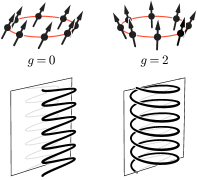
Figure 1: Geometric characterization of the gyromagnetic ratio $g$. A charged spinning particle exhibits both orbital and spin precession in an external “magnetic” field. If $g{\hskip 1.00006pt=\hskip 1.00006pt}2$, the two precessions are locally synchronized; such a motion appears as an isotropic spiral trajectory as seen in the particle’s spin-space-time. In contrast, $g{\hskip 1.00006pt=\hskip 1.00006pt}0$ translates to a “flattened” sinusoidal curve. Notice how spin-space-time offers a new angle on spin precession. The visual reasoning suggests that the field strength should somehow extend into the complex. The isotropy of $g{\hskip 1.00006pt=\hskip 1.00006pt}2$ points to the equal blending of all $dx$-$dy$ components in $dz{\hskip 1.00006pt{\wedge}\,}dz$; the “flatness” of $g{\hskip 1.00006pt=\hskip 1.00006pt}0$ points to the reality of $dx{\hskip 1.00006pt{\wedge}\,}dx$.

Earthly equation of motion and $\bm{C_{\ell}{\,\hskip 1.00006pt=\hskip 1.00006pt\,}1}$

Finally, we spell out the constant-mass earthly equation of motion at $\mathcal{O}(\omega^{\prime 1})$ in the vectorial language by taking “ $2\hskip 0.50003pt{\operatorname{Re}}$” to (56):

$$\begin{split}m_{0}\hskip 1.00006pt\dot{p}_{m}\simeq-\hskip 1.00006ptp_{n}\hskip 1.00006pt(\hskip 0.50003pt\phi^{+}(z){\,+\,}\phi^{-}({\bar{z}})\hskip 0.12497pt)^{n}{}_{m}&\,,\quad m_{0}\hskip 1.00006pt\dot{\Lambda}^{m}{}_{a}\simeq\hskip 1.00006pt(\hskip 0.50003pt\phi^{+}(z){\,+\,}\phi^{-}({\bar{z}})\hskip 0.12497pt)^{m}{}_{n}\hskip 1.00006pt\Lambda^{n}{}_{a}\,,\\ m_{0}\dot{x}^{m}\simeq p^{m}-\hskip 1.00006pt*(\hskip 0.50003pt\phi^{+}(z){\,+\,}\phi^{-}({\bar{z}})\hskip 0.12497pt)^{m}{}_{n}\hskip 1.00006pty^{n}&\,,\quad m_{0}\hskip 1.00006pt\dot{y}^{m}\simeq\hskip 1.00006pt(\hskip 0.50003pt\phi^{+}(z){\,+\,}\phi^{-}({\bar{z}})\hskip 0.12497pt)^{m}{}_{n}\hskip 1.00006pty^{n}\,.\end{split}$$ (58)

The orbital ($p_{m}$) and spin ($\Lambda^{m}{}_{a}$, $y^{m}$) precessions are synchronized at $\mathcal{O}(\phi^{1})$ (Figure 1). Taylor-expanding the fields around the real section, we recognize $C_{\ell}{\,\hskip 1.00006pt=\hskip 1.00006pt\,}1$ (see (193)), in particular $g{\,=\,}2$ at $\mathcal{O}(y^{1})$ and $\kappa{\,=\,}1$ at $\mathcal{O}(y^{2})$ by referring to TBMT and MPTD equations.

Spin as a chiral Wick rotation of deviation

Meanwhile, note that the evolution of $x^{m}$ deviates from this synchronized precession ($p^{m}$) by a zitterbewegung that is “dual” to the spin precession ($-{\ast\phi}{}^{m}{}_{n}\hskip 1.00006pty^{n}$). This zitterbewegung reflects the “spin-induced spacetime noncommutativity” (15) and its resolution in the complex combinations: The covariant spin gauge fixing has put deviation in real spacetime and spin on an equal footing. We give a closer look at this dual relationship between deviation and spin in [83].

3.2 Non-minimal equation of motion

We now return to the generic class of spin-space-time symplectic perturbations (32).

Maximally non-minimal coupling

A typical example of a non-holomorphic spin-space-time symplectic perturbation is a closed two-form that localizes on the spacetime:

$$\begin{split}\omega^{\prime+}&={\textstyle\frac{1}{2}\,}\phi^{+}_{mn}(x)\hskip 1.00006pt{d{x}^{m}\wedge d{x}^{n}}\,,\\ &={\textstyle\frac{1}{4}\,}\phi^{+}_{mn}(x)\hskip 1.00006pt\big{(}{\textstyle\frac{1}{2}}\hskip 1.00006pt{d{z}^{m}\wedge d{z}^{n}}+dz^{m}{\hskip 0.50003pt\otimes\hskip 1.00006pt\hskip 0.50003pt}d{\bar{z}}^{n}+d{\bar{z}}^{m}{\hskip 0.50003pt\otimes\hskip 1.00006pt\hskip 0.50003pt}dz^{n}+{\textstyle\frac{1}{2}}\hskip 1.00006pt{d{{\bar{z}}}^{m}\wedge d{{\bar{z}}}^{n}}\big{)}\,,\\ &=:\frac{1}{4}\left(\,\includegraphics[valign={c}]{figs/insert0+ww.pdf}+\includegraphics[valign={c}]{figs/insert0+wb.pdf}+\includegraphics[valign={c}]{figs/insert0+bw.pdf}+\includegraphics[valign={c}]{figs/insert0+bb.pdf}\,\right)\,.\end{split}$$ (59)

In terms of (32), we have

$${{}^{0}\omega^{\prime+}_{mn}}\hskip 1.00006pt=\hskip 1.00006pt{{}^{1}\omega^{\prime+}_{mn}}\hskip 1.00006pt=\hskip 1.00006pt{{}^{2}\omega^{\prime+}_{mn}}\hskip 1.00006pt=\hskip 1.00006pt{\textstyle\frac{1}{4}}\hskip 1.00006pt\phi^{+}_{mn}(x)\,.$$ (60)

At first sight, the symplectic perturbation (59) may seem like a “minimal” coupling prescription because it simply brings the “field strength” two-form without any post-processing, such as the Newman-Janis shift. However, in the holomorphic/anti-holomorphic basis, it looks rather complicated. In fact, the zig-zag representation discloses its maximally non-minimal nature. We find three new types of zig-zag vertices, which cause a proliferation of zig-zag interaction scenarios:

$$\{{\,\,\,\,\,},{\bar{\Delta}}\}=\, \includegraphics[valign={c}]{figs/l.pdf}\includegraphics[valign={c}]{figs/xD-b.pdf}-\includegraphics[valign={c}]{figs/l-b.pdf}\includegraphics[valign={c}]{figs/0+ww.pdf}\includegraphics[valign={c}]{figs/xD-b.pdf}-\includegraphics[valign={c}]{figs/l.pdf}\includegraphics[valign={c}]{figs/0+bw.pdf}\includegraphics[valign={c}]{figs/xD-b.pdf}$$ (61)

$$+\includegraphics[valign={c}]{figs/l-b.pdf}\includegraphics[valign={c}]{figs/0+wb.pdf}\includegraphics[valign={c}]{figs/0+ww.pdf}\includegraphics[valign={c}]{figs/xD-b.pdf}+\includegraphics[valign={c}]{figs/l.pdf}\includegraphics[valign={c}]{figs/0+bb.pdf}\includegraphics[valign={c}]{figs/0+ww.pdf}\includegraphics[valign={c}]{figs/xD-b.pdf}+\includegraphics[valign={c}]{figs/l-b.pdf}\includegraphics[valign={c}]{figs/0+ww.pdf}\includegraphics[valign={c}]{figs/0+bw.pdf}\includegraphics[valign={c}]{figs/xD-b.pdf}+\includegraphics[valign={c}]{figs/l.pdf}\includegraphics[valign={c}]{figs/0+bw.pdf}\includegraphics[valign={c}]{figs/0+bw.pdf}\includegraphics[valign={c}]{figs/xD-b.pdf}+\cdots\vphantom{\leavevmode\hbox{\raise-8.61108pt\hbox{\set@color\resizebox{}{}{{\leavevmode\hbox{\set@color{$0$}}}}}}}\,,$$

$$\{{\,\,\,\,\,},\Delta\}=\, \includegraphics[valign={c}]{figs/l-b.pdf}\includegraphics[valign={c}]{figs/xD.pdf}-\includegraphics[valign={c}]{figs/l-b.pdf}\includegraphics[valign={c}]{figs/0+wb.pdf}\includegraphics[valign={c}]{figs/xD.pdf}-\includegraphics[valign={c}]{figs/l.pdf}\includegraphics[valign={c}]{figs/0+bb.pdf}\includegraphics[valign={c}]{figs/xD.pdf}$$ (62)

$$+\includegraphics[valign={c}]{figs/l-b.pdf}\includegraphics[valign={c}]{figs/0+wb.pdf}\includegraphics[valign={c}]{figs/0+wb.pdf}\includegraphics[valign={c}]{figs/xD.pdf}+\includegraphics[valign={c}]{figs/l.pdf}\includegraphics[valign={c}]{figs/0+bb.pdf}\includegraphics[valign={c}]{figs/0+wb.pdf}\includegraphics[valign={c}]{figs/xD.pdf}+\includegraphics[valign={c}]{figs/l-b.pdf}\includegraphics[valign={c}]{figs/0+ww.pdf}\includegraphics[valign={c}]{figs/0+bb.pdf}\includegraphics[valign={c}]{figs/xD.pdf}+\includegraphics[valign={c}]{figs/l.pdf}\includegraphics[valign={c}]{figs/0+bw.pdf}\includegraphics[valign={c}]{figs/0+bb.pdf}\includegraphics[valign={c}]{figs/xD.pdf}+\cdots\,.$$

The expansions never truncate, regardless of whether one assumes pure self-duality or not. Besides, one can argue that $\phi^{+}_{mn}(x)$ actually contains an infinite number of derivative couplings as $\phi^{+}_{mn}(z)-iy^{r}\phi^{+}_{mn,r}(z)+\cdots$ if one takes the holomorphic Minkowski space as more fundamental than the real spacetime. In any respect, this is by no means “minimal.”

Maximally non-minimal spin precession: $\bm{C_{\ell\hskip 0.35002pt>\hskip 0.35002pt0}{\hskip 1.00006pt\,=\,\hskip 1.00006pt}0}$

Let us compute the $\mathcal{O}(\omega^{\prime 1})$ equation of motion that follows from (59). First of all, we find

$$-\includegraphics[valign={c}]{figs/l-b.pdf}\includegraphics[valign={c}]{figs/0+ww.pdf}\includegraphics[valign={c}]{figs/xD-b.pdf} =\,\,\frac{(-2)}{\Delta}\,\omega^{\prime{\dot{\beta}}}{}_{{\dot{\alpha}}}(x)\left({\bar{\lambda}}_{I{\dot{\beta}}}\hskip 1.00006pt\hskip 0.50003pt\frac{\partial}{\partial{\bar{\lambda}}_{I{\dot{\alpha}}}}+2iy^{{\dot{\alpha}}{\gamma}}\frac{\partial}{\partial{\bar{z}}^{{\dot{\beta}}{\gamma}}}\right)\,,$$ (63a)

$$-\includegraphics[valign={c}]{figs/l-b.pdf}\includegraphics[valign={c}]{figs/0+wb.pdf}\includegraphics[valign={c}]{figs/xD.pdf} =\,\,\frac{(-2)}{{\bar{\Delta}}}\,\omega^{\prime{\dot{\beta}}}{}_{{\dot{\alpha}}}(x)\left({\bar{\lambda}}_{I{\dot{\beta}}}\hskip 1.00006pt\hskip 0.50003pt\frac{\partial}{\partial{\bar{\lambda}}_{I{\dot{\alpha}}}}+2iy^{{\dot{\alpha}}{\gamma}}\frac{\partial}{\partial{\bar{z}}^{{\dot{\beta}}{\gamma}}}\right)\,,$$ (63b)

$$-\includegraphics[valign={c}]{figs/l.pdf}\includegraphics[valign={c}]{figs/0+bw.pdf}\includegraphics[valign={c}]{figs/xD-b.pdf} =\,\,\frac{(-2)}{\Delta}\,p_{\alpha{\dot{\alpha}}}\hskip 1.00006pt\omega^{\prime{\dot{\alpha}}}{}_{\dot{\beta}}(x)\hskip 0.50003pt(p^{-1})^{{\dot{\beta}}\beta}\left(\lambda_{\beta}{}^{I}\hskip 0.50003pt\frac{\partial}{\partial\lambda_{\alpha}{}^{I}}-2iy^{{\dot{{\gamma}}}\alpha}\hskip 0.50003pt\frac{\partial}{\partial z^{{\dot{{\gamma}}}\beta}}\right)\,,$$ (63c)

$$-\includegraphics[valign={c}]{figs/l.pdf}\includegraphics[valign={c}]{figs/0+bb.pdf}\includegraphics[valign={c}]{figs/xD.pdf} =\,\,\frac{(-2)}{{\bar{\Delta}}}\,p_{\alpha{\dot{\alpha}}}\hskip 1.00006pt\omega^{\prime{\dot{\alpha}}}{}_{\dot{\beta}}(x)\hskip 0.50003pt(p^{-1})^{{\dot{\beta}}\beta}\left(\lambda_{\beta}{}^{I}\hskip 0.50003pt\frac{\partial}{\partial\lambda_{\alpha}{}^{I}}-2iy^{{\dot{{\gamma}}}\alpha}\hskip 0.50003pt\frac{\partial}{\partial z^{{\dot{{\gamma}}}\beta}}\right)\,.$$ (63d)

The first two lines are equal to (54) on the mass-shell constraint surface. The last two lines involve an interesting combination $p_{\alpha{\dot{\alpha}}}\hskip 1.00006pt\omega^{\prime{\dot{\alpha}}}{}_{\dot{\beta}}\hskip 0.50003pt(p^{-1})^{{\dot{\beta}}\beta}$. This particular sandwiching has a geometrical interpretation as a reflection across the momentum direction:

$$\begin{split}(p\hskip 1.00006pt{\bar{\sigma}}^{m}p)_{\alpha{\dot{\alpha}}}=p^{2}\hskip 1.00006ptI^{m}{}_{n}(\sigma^{n})_{\alpha{\dot{\alpha}}}&\,,\quad(p^{-1}\sigma^{m}\hskip 1.00006ptp^{-1})^{{\dot{\alpha}}\alpha}=p^{-2}\hskip 1.00006ptI^{m}{}_{n}({\bar{\sigma}}^{n})^{{\dot{\alpha}}\alpha}\,,\\ (p\hskip 1.00006pt{\bar{\sigma}}^{mn}p^{-1})_{\alpha}{}^{\beta}=-I^{m}{}_{r}I^{n}{}_{s}(\sigma^{rs})_{\alpha}{}^{\beta}&\,,\quad(p^{-1}\sigma^{mn}\hskip 1.00006ptp)^{\dot{\alpha}}{}_{\dot{\beta}}=-I^{m}{}_{r}I^{n}{}_{s}({\bar{\sigma}}^{rs})^{\dot{\alpha}}{}_{\dot{\beta}}\,,\\ I^{m}{}_{n}:=\delta^{m}{}_{n}-2p^{m}p_{n}/p^{2}&\,,\quad\varepsilon_{pqkl}\hskip 0.50003ptI^{p}{}_{m}I^{q}{}_{n}I^{k}{}_{r}I^{l}{}_{s}=-\varepsilon_{mnrs}\,.\end{split}$$ (64)

These identities are easily understood if one recalls the inversive geometry of the Clifford/conformal algebra [170] and that the inversion map $p^{m}\mapsto p^{m}/p^{2}$ has the Jacobian $p^{-2}(\delta^{m}{}_{n}-2p^{m}p_{n}/p^{2})$. For later use, we define a notation “${{}_{\mathcal{I}}F_{mn}}$” for two-forms $F_{mn}$:

$$\begin{split}{{}_{\mathcal{I}}F_{mn}}:=F_{rs}\hskip 1.00006ptI^{r}{}_{m}I^{s}{}_{n}{\quad\implies\quad}\left\{{\begin{array}[]{rl}p_{\alpha{\dot{\alpha}}}\hskip 1.00006ptF^{\dot{\alpha}}{}_{\dot{\beta}}\hskip 1.00006pt(p^{-1})^{{\dot{\beta}}\beta}&=-(_{\mathcal{I}}F)_{\alpha}{}^{\beta}\,,\\ (p^{-1})^{{\dot{\alpha}}\alpha}\hskip 1.00006ptF_{\alpha}{}^{\beta}\hskip 1.00006ptp_{\beta{\dot{\beta}}}&=-(_{\mathcal{I}}F)^{\dot{\alpha}}{}_{\dot{\beta}}\,.\end{array}}\right.\end{split}$$ (65)

The heavenly equation of motion follows from collecting (LABEL:eq:holomorhictranslations), (63), and (65). Then the earthly equation of motion is then obtained by simply replacing $\phi^{+}_{mn}(x)$ with $\phi_{mn}(x)$, as the real perturbation $dx{\hskip 1.00006pt{\wedge}\,}dx$ acts “symmetrically” on the zig and zag sectors:

$$\begin{split}m_{0}\hskip 1.00006pt\dot{p}_{m}\simeq-p_{n}\hskip 1.00006pt\phi{}^{n}{}_{m}(x)\,,\quad&\textstyle m_{0}\hskip 1.00006pt\dot{\Lambda}^{m}{}_{a}\simeq-\frac{1}{{m_{0}}^{2}}\hskip 1.00006ptp^{m}p^{r}\phi_{rs}(x)\hskip 1.00006pt\Lambda^{s}{}_{a}\,,\\ m_{0}\dot{x}^{m}\simeq p^{m}-(\eta^{mr}{-\hskip 1.00006pt}p^{m}p^{r}/p^{2})\hskip 1.00006pt{\ast\phi_{rs}}(x)\hskip 1.00006pty^{s}\,,\quad&\textstyle m_{0}\hskip 1.00006pt\dot{y}^{m}\simeq-\frac{1}{{m_{0}}^{2}}\hskip 1.00006ptp^{m}p^{r}\phi_{rs}(x)\hskip 1.00006pty^{s}\,.\end{split}$$ (66)

(66) agrees with (193) if $C_{\ell\hskip 0.35002pt>\hskip 0.35002pt0}{\hskip 1.00006pt\,=\,\hskip 1.00006pt}0$: $g{\,=\,}0$ for TBMT and $\kappa{\,=\,}0$ for MPTD. Evidently, the precession behaviors of $p_{m}$ and $y^{m}$ are not synchronized.

To sum up, our formalism is the simplest with the holomorphic symplectic perturbation (35) and gets “maximally” complicated with (59): all the $(2,0)$-, $(1,1)$-, and $(0,2)$-parts appear in (59) with an “equal” magnitude. This contrasts sharply with the traditional approach, which treats the real-supported symplectic structure (59) as the default and implements the minimal gyromagnetic ratio $g{\,=\,}2$ by an additional “non-minimal” spin interaction Hamiltonian $H^{\prime}=q\vec{B}{\hskip 1.00006pt\cdot\hskip 1.00006pt}\vec{S}$ (and similarly for $\kappa$). While the traditional approach creates an unfortunate discrepancy between the classical formalism and the amplitudes-level understanding of [66, 3], our perturbation theory is literally minimal at the true minimal coupling $C_{\ell}{\hskip 1.00006pt\,=\,\hskip 1.00006pt}1$ ($g{\,=\,}2$, $\kappa{\,=\,}1$, $\cdots$). Therefore, we argue that our “zig-zag” formulation provides a rationale for identifying $C_{\ell}{\hskip 1.00006pt\,=\,\hskip 1.00006pt}1$ as the true minimal coupling and $C_{\ell\hskip 0.35002pt>\hskip 0.35002pt0}{\hskip 1.00006pt\,=\,\hskip 1.00006pt}0$ ($g{\,=\,}2$, $\kappa{\,=\,}0$, $\cdots$) as the maximally non-minimal coupling already at the classical level. The massive twistor representation of massive spinning particles has guided us to do so, as the zig-zag structure—already inherent in the free theory as the skew-diagonalization of the Poisson bracket—asserts that one should understand everything in the complex basis.

Generic heavenly equation of motion

Finally, we spell out the $\mathcal{O}(\omega^{\prime 1})$ heavenly equation of motion that follows from the generic perturbation (32a). It is easily obtainable by recycling the calculations of (63):

$$\begin{split}m_{0}\hskip 0.50003pt\frac{d}{d\tau}\,\simeq\,\hskip 1.00006pt\frac{p^{{\dot{\alpha}}\alpha}}{-2}\hskip 0.50003pt\frac{\partial}{\partial x^{{\dot{\alpha}}\alpha}}&{}+(\hskip 0.50003pt{{}^{0+1}\omega^{\prime}})^{\dot{\beta}}{}_{\dot{\alpha}}\left({\bar{\lambda}}_{I{\dot{\beta}}}\hskip 1.00006pt\frac{\partial}{\partial{\bar{\lambda}}_{I{\dot{\alpha}}}}+2iy^{{\dot{\alpha}}{\gamma}}\frac{\partial}{\partial{\bar{z}}^{{\dot{\beta}}{\gamma}}}\right)\\ &{}+({{}^{1+2}\mathllap{\leavevmode\hbox{\raise-0.86108pt\hbox{\set@color\resizebox{}{}{{\leavevmode\hbox{\set@color{${}_{\mathcal{I}}\hskip 0.50003pt$}}}}}}}\omega^{\prime}})_{\alpha}{}^{\beta}\left(-\lambda_{\beta}{}^{I}\hskip 0.50003pt\frac{\partial}{\partial\lambda_{\alpha}{}^{I}}+2iy^{{\dot{{\gamma}}}\alpha}\hskip 0.50003pt\frac{\partial}{\partial z^{{\dot{{\gamma}}}\beta}}\right)\,,\end{split}$$ (67)

where ${{}^{0+1}\omega^{\prime+}_{mn}}:={{}^{0}\omega^{\prime+}_{mn}}+{{}^{1}\omega^{\prime+}_{mn}}$, ${{}^{1+2}\omega^{\prime+}_{mn}}:={{}^{1}\omega^{\prime+}_{mn}}+{{}^{2}\omega^{\prime+}_{mn}}$. In other words,

$$\begin{split}m_{0}\hskip 0.50003pt\dot{\lambda}_{\alpha}{}^{I}\simeq-(^{1+2}\mathllap{\leavevmode\hbox{\raise-0.86108pt\hbox{\set@color\resizebox{}{}{{\leavevmode\hbox{\set@color{${}_{\mathcal{I}}\hskip 0.50003pt$}}}}}}}\omega^{\prime})_{\alpha}{}^{\beta}\hskip 0.50003pt\lambda_{\beta}{}^{I}&\,,\quad m_{0}\hskip 0.50003pt\dot{z}^{{\dot{\alpha}}\alpha}\simeq{\textstyle\frac{1}{-2}}{p^{{\dot{\alpha}}\alpha}}+2i\hskip 0.50003pty^{{\dot{\alpha}}\beta}\hskip 0.50003pt(^{1+2}\mathllap{\leavevmode\hbox{\raise-0.86108pt\hbox{\set@color\resizebox{}{}{{\leavevmode\hbox{\set@color{${}_{\mathcal{I}}\hskip 0.50003pt$}}}}}}}\omega^{\prime})_{\beta}{}^{\alpha}\,,\\ m_{0}\hskip 0.50003pt\dot{{\bar{\lambda}}}_{I{\dot{\alpha}}}\simeq{\bar{\lambda}}_{I{\dot{\beta}}}\hskip 0.50003pt(\hskip 0.50003pt^{0+1}\omega^{\prime})^{\dot{\beta}}{}_{\dot{\alpha}}&\,,\quad m_{0}\hskip 0.50003pt\dot{{\bar{z}}}^{{\dot{\alpha}}\alpha}\simeq{\textstyle\frac{1}{-2}}{p^{{\dot{\alpha}}\alpha}}+2i\hskip 1.00006pt(\hskip 0.50003pt^{0+1}\omega^{\prime})^{\dot{\alpha}}{}_{\dot{\beta}}\hskip 1.00006pty^{{\dot{\beta}}\alpha}\,.\end{split}$$ (68)

In the vectorial language, we find

$$\begin{split}m_{0}\hskip 1.00006pt\dot{p}_{m}&\simeq\big{(}\hskip 0.50003pt{{{}^{0+1}\omega^{\prime+}}}-{{{}^{1+2}\mathllap{\leavevmode\hbox{\raise-0.86108pt\hbox{\set@color\resizebox{}{}{{\leavevmode\hbox{\set@color{${}_{\mathcal{I}}\hskip 0.50003pt$}}}}}}}\omega^{\prime+}}}\big{)}{}_{m}{}^{n}\hskip 1.00006ptp_{n}\simeq-p_{n}\hskip 1.00006pt\omega^{\prime+}{}^{n}{}_{m}\,,\\ m_{0}\hskip 1.00006pt\dot{\Lambda}^{m}{}_{a}&\simeq\big{(}\hskip 0.50003pt{{{}^{0+1}\omega^{\prime+}}}-{{{}^{1+2}\mathllap{\leavevmode\hbox{\raise-0.86108pt\hbox{\set@color\resizebox{}{}{{\leavevmode\hbox{\set@color{${}_{\mathcal{I}}\hskip 0.50003pt$}}}}}}}\omega^{\prime+}}}\big{)}{}^{m}{}_{n}\hskip 1.00006pt\Lambda^{n}{}_{a}\,,\\ m_{0}\hskip 1.00006pt\dot{y}^{m}&\simeq\big{(}\hskip 0.50003pt{{{}^{0+1}\omega^{\prime+}}}-{{{}^{1+2}\mathllap{\leavevmode\hbox{\raise-0.86108pt\hbox{\set@color\resizebox{}{}{{\leavevmode\hbox{\set@color{${}_{\mathcal{I}}\hskip 0.50003pt$}}}}}}}\omega^{\prime+}}}\big{)}{}^{m}{}_{n}\hskip 1.00006pty^{n}\,,\\ m_{0}\dot{x}^{m}&\simeq p^{m}-{\ast}\big{(}\hskip 0.50003pt{{{}^{0+1}\omega^{\prime+}}}-{{{}^{1+2}\mathllap{\leavevmode\hbox{\raise-0.86108pt\hbox{\set@color\resizebox{}{}{{\leavevmode\hbox{\set@color{${}_{\mathcal{I}}\hskip 0.50003pt$}}}}}}}\omega^{\prime+}}}\big{)}{}^{m}{}_{n}\hskip 1.00006pty^{n}\,.\end{split}$$ (69)

Note that _I and $\ast$ anti-commute.

Arbitrary g value

Before moving on to the Wilson coefficients, let us discuss two more examples for further concreteness. First, it is instructive to think of a certain interpolation between the two extremes (35) and (59):

$$\begin{split}\omega^{\prime+}&{}=\phi_{\smash{{\dot{\alpha}}{\dot{\beta}}}\vphantom{\beta}}({x{\hskip 1.00006pt+\hskip 1.00006pt}igy/2})\,\hskip 0.50003pt\epsilon_{\alpha\beta}\hskip 1.00006ptd(x{\hskip 1.00006pt+\hskip 1.00006pt}igy/2)^{{\dot{\alpha}}\alpha}{\hskip 1.00006pt{\wedge}\,}d(x{\hskip 1.00006pt+\hskip 1.00006pt}igy/2)^{{\dot{\beta}}\beta}\,,\\ &{}=:{\frac{1}{4}\bigg{(}\smash{(1+g/2)^{2}\,\hskip 1.00006pt\includegraphics[valign={c}]{figs/insertg+ww.pdf}\hskip 1.00006pt+(1-(g/2)^{2})\,\hskip 1.00006pt\includegraphics[valign={c}]{figs/insertg+wb.pdf}\hskip 1.00006pt+(1-(g/2)^{2})\,\hskip 1.00006pt\includegraphics[valign={c}]{figs/insertg+bw.pdf}\hskip 1.00006pt+(1-g/2)^{2}\,\hskip 1.00006pt\includegraphics[valign={c}]{figs/insertg+bb.pdf}\hskip 1.00006pt\,}\bigg{)}}\,,\\ \omega^{\prime-}&{}=\phi_{\smash{{\dot{\alpha}}{\dot{\beta}}}\vphantom{\beta}}({x{\hskip 1.00006pt-\hskip 1.00006pt}igy/2})\,\hskip 0.50003pt{\bar{\epsilon}}_{\smash{{\dot{\alpha}}{\dot{\beta}}}\vphantom{\beta}}\hskip 1.00006ptd(x{\hskip 1.00006pt-\hskip 1.00006pt}igy/2)^{{\dot{\alpha}}\alpha}{\hskip 1.00006pt{\wedge}\,}d(x{\hskip 1.00006pt-\hskip 1.00006pt}igy/2)^{{\dot{\beta}}\beta}\,,\\ &{}=:{\frac{1}{4}\bigg{(}(1+g/2)^{2}\,\hskip 1.00006pt\leavevmode\hbox{$\vbox{\hbox{\resizebox{}{}{{\leavevmode\hbox{\set@color{{\includegraphics[rotate=180]{figs/insertg+bb.pdf}}}}}}}}$}\hskip 1.00006pt+(1-(g/2)^{2})\,\hskip 1.00006pt\leavevmode\hbox{$\vbox{\hbox{\resizebox{}{}{{\leavevmode\hbox{\set@color{{\includegraphics[rotate=180]{figs/insertg+wb.pdf}}}}}}}}$}\hskip 1.00006pt+(1-(g/2)^{2})\,\hskip 1.00006pt\leavevmode\hbox{$\vbox{\hbox{\resizebox{}{}{{\leavevmode\hbox{\set@color{{\includegraphics[rotate=180]{figs/insertg+bw.pdf}}}}}}}}$}\hskip 1.00006pt+(1-g/2)^{2}\,\hskip 1.00006pt\leavevmode\hbox{$\vbox{\hbox{\resizebox{}{}{{\leavevmode\hbox{\set@color{{\includegraphics[rotate=180]{figs/insertg+ww.pdf}}}}}}}}$}\hskip 1.00006pt\,\bigg{)}}\,.\end{split}$$ (70)

For reference, we have spelled out the anti-self-dual counterpart as well. As indicated in the diagrammatic format, each part of $\omega^{\prime+}$ is given as

$$\begin{split}{{}^{0}\omega^{\prime+}_{mn}}&\hskip 1.00006pt=\hskip 1.00006pt\hskip 0.24994pt{\textstyle\frac{1}{4}}\hskip 0.50003pt(1+g/2)^{2}\,\phi^{+}_{mn}(x{\hskip 1.00006pt+\hskip 1.00006pt}igy/2)\,,\\ {{}^{1}\omega^{\prime+}_{mn}}&\hskip 1.00006pt=\hskip 1.00006pt\hskip 0.24994pt{\textstyle\frac{1}{4}}\hskip 0.50003pt(1-(g/2)^{2})\,\phi^{+}_{mn}(x{\hskip 1.00006pt+\hskip 1.00006pt}igy/2)\,,\\ {{}^{2}\omega^{\prime+}_{mn}}&\hskip 1.00006pt=\hskip 1.00006pt\hskip 0.24994pt{\textstyle\frac{1}{4}}\hskip 0.50003pt(1-g/2)^{2}\,\phi^{+}_{mn}(x{\hskip 1.00006pt+\hskip 1.00006pt}igy/2)\,.\end{split}$$ (71)

The heavenly equation of motion (69) boils down to

$$\begin{split}m_{0}\hskip 1.00006pt\dot{p}_{m}&=-p_{n}\hskip 1.00006pt\phi^{+}{}^{n}{}_{m}(x{\hskip 1.00006pt+\hskip 1.00006pt}igy/2)\,,\\ m_{0}\hskip 0.50003pt\hskip 0.24994pt\dot{\Lambda}^{m}{}_{a}&=\bigg{(}\hskip 1.00006pt{\frac{g}{2}\,\phi^{+}{}^{m}{}_{n}(x{\hskip 1.00006pt+\hskip 1.00006pt}igy/2)-\frac{2{\hskip 1.00006pt-\hskip 1.00006pt}g}{2}\,\frac{\hskip 0.24994pt{p^{m}p_{l}}\hskip 0.24994pt}{m^{2}}\,\phi^{+}{}^{l}{}_{n}(x{\hskip 1.00006pt+\hskip 1.00006pt}igy/2)}\bigg{)}\hskip 1.00006pt\Lambda^{n}{}_{a}\,,\\ m_{0}\hskip 1.00006pt\dot{y}^{m}&=\bigg{(}\hskip 1.00006pt{\frac{g}{2}\,\phi^{+}{}^{m}{}_{n}(x{\hskip 1.00006pt+\hskip 1.00006pt}igy/2)-\frac{2{\hskip 1.00006pt-\hskip 1.00006pt}g}{2}\,\frac{\hskip 0.24994pt{p^{m}p_{l}}\hskip 0.24994pt}{m^{2}}\,\phi^{+}{}^{l}{}_{n}(x{\hskip 1.00006pt+\hskip 1.00006pt}igy/2)}\bigg{)}\hskip 1.00006pty^{n}\,,\\ m_{0}\dot{x}^{m}&=p^{m}+\bigg{(}\hskip 1.00006pt{-{\ast}\phi^{+}{}^{m}{}_{n}(x{\hskip 1.00006pt+\hskip 1.00006pt}igy/2)-\frac{2{\hskip 1.00006pt-\hskip 1.00006pt}g}{2}\,\frac{\hskip 0.24994pt{p^{m}p_{l}}\hskip 0.24994pt}{m^{2}}\,{\ast}\phi^{+}{}^{l}{}_{n}(x{\hskip 1.00006pt+\hskip 1.00006pt}igy/2)}\bigg{)}\hskip 1.00006pty^{n}\,.\end{split}$$ (72)

Replacing $\phi^{+}{}^{m}{}_{n}(x{\hskip 1.00006pt+\hskip 1.00006pt}igy/2)$ with $\phi^{+}{}^{m}{}_{n}(x)+(g/2)\hskip 1.00006pt{\ast}((y{\hskip 1.00006pt\cdot\hskip 1.00006pt}\partial)\phi^{+}(x))^{m}{}_{n}+\cdots$, one finds that (72) reproduces the arbitrary-$g$ TBMT equation (191) in the small spin-derivative limit $(y{\hskip 0.50003pt\cdot\hskip 0.50003pt}\partial)\hskip 0.50003pt\phi\ll\phi$. It is interesting that the projector structure of the TBMT equation derives from the reflection matrix $I^{m}{}_{n}$, which traces back to the inversive geometry of the Clifford algebra (cf. [171]).

Antipodal minimal coupling

When we were introducing the ansatz (35), the reader may have questioned the possibility of extending the self-dual part anti-holomorphically:

$$\begin{split}\omega^{\prime+}&\hskip 0.50003pt=\,\hskip 1.00006pt{\bar{\phi}}_{\smash{\alpha\beta}\vphantom{\beta}}({\bar{z}})\hskip 1.00006pt{\bar{\epsilon}}_{\smash{{\dot{\alpha}}{\dot{\beta}}}\vphantom{\beta}}({d{\bar{z}}^{{\dot{\alpha}}\alpha}\wedge d{\bar{z}}^{{\dot{\beta}}\beta}})\,\,=\,\,\hskip 0.50003pt\includegraphics[valign={c},scale={1.0}]{figs/insertA+.pdf}\hskip 0.50003pt\,,\\ \omega^{\prime-}&\hskip 0.50003pt=\,\hskip 1.00006pt\phi_{\smash{{\dot{\alpha}}{\dot{\beta}}}\vphantom{\beta}}(z)\hskip 1.00006pt\epsilon_{\smash{\alpha\beta}\vphantom{\beta}}({dz^{{\dot{\alpha}}\alpha}\wedge dz^{{\dot{\beta}}\beta}})\,\,=\,\,\hskip 0.50003pt\includegraphics[valign={c},scale={1.0}]{figs/insertA-.pdf}\hskip 0.50003pt\,.\end{split}$$ (73)

In terms of (70), this corresponds to $g{\,=\,}-2$. The combinatorics of the zig-zag expansions is the same as that of the minimal coupling:

$$\begin{split}&\omega^{-1}=\includegraphics[valign={c}]{figs/l.pdf}\includegraphics[valign={c}]{figs/r-b.pdf}+\includegraphics[valign={c}]{figs/l-b.pdf}\includegraphics[valign={c}]{figs/r.pdf}-\includegraphics[valign={c}]{figs/l.pdf}\includegraphics[valign={c}]{figs/A+.pdf}\includegraphics[valign={c}]{figs/r.pdf}\quad\text{(heavenly)}\,,\\ &{\begin{array}[]{rl}\omega^{-1}=\includegraphics[valign={c}]{figs/l.pdf}\includegraphics[valign={c}]{figs/r-b.pdf}+\includegraphics[valign={c}]{figs/l-b.pdf}\includegraphics[valign={c}]{figs/r.pdf}{}&{}-\includegraphics[valign={c}]{figs/l.pdf}\includegraphics[valign={c}]{figs/A+.pdf}\includegraphics[valign={c}]{figs/r.pdf}-\includegraphics[valign={c}]{figs/l-b.pdf}\includegraphics[valign={c}]{figs/A-.pdf}\includegraphics[valign={c}]{figs/r-b.pdf}\\ {}\hfil&{}+\includegraphics[valign={c}]{figs/l-b.pdf}\includegraphics[valign={c}]{figs/A-.pdf}\includegraphics[valign={c}]{figs/A+.pdf}\includegraphics[valign={c}]{figs/r.pdf}+\includegraphics[valign={c}]{figs/l.pdf}\includegraphics[valign={c}]{figs/A+.pdf}\includegraphics[valign={c}]{figs/A-.pdf}\includegraphics[valign={c}]{figs/r-b.pdf}+\cdots\quad\text{(earthly)}\,.\end{array}}\end{split}$$ (74)

We call this case “antipodal minimal coupling,” in the sense that its equation of motion is a certain “inversion” of that of the minimal coupling. The self-dual heavenly equation of motion reads

$$\begin{split}m_{0}\hskip 0.50003pt\dot{\lambda}_{\alpha}{}^{I}=-(^{\phantom{\hskip 0.17496pt\mathcal{I}}}\mathllap{\leavevmode\hbox{\raise-0.86108pt\hbox{\set@color\resizebox{}{}{{\leavevmode\hbox{\set@color{${}_{\mathcal{I}}\hskip 0.50003pt$}}}}}}}{\bar{\phi}}({\bar{z}}))_{\alpha}{}^{\beta}\hskip 0.50003pt\lambda_{\beta}{}^{I}&\,,\quad m_{0}\hskip 0.50003pt\dot{z}^{{\dot{\alpha}}\alpha}={\textstyle\frac{1}{-2}}{p^{{\dot{\alpha}}\alpha}}+2i\hskip 0.50003pty^{{\dot{\alpha}}\beta}\hskip 0.50003pt(^{\phantom{\hskip 0.17496pt\mathcal{I}}}\mathllap{\leavevmode\hbox{\raise-0.86108pt\hbox{\set@color\resizebox{}{}{{\leavevmode\hbox{\set@color{${}_{\mathcal{I}}\hskip 0.50003pt$}}}}}}}{\bar{\phi}}({\bar{z}}))_{\beta}{}^{\alpha}\,,\\ m_{0}\hskip 0.50003pt\dot{{\bar{\lambda}}}_{I{\dot{\alpha}}}=0&\,,\quad m_{0}\hskip 0.50003pt\dot{{\bar{z}}}^{{\dot{\alpha}}\alpha}={\textstyle\frac{1}{-2}}{p^{{\dot{\alpha}}\alpha}}\,.\end{split}$$ (75)

One finds the same equations by taking complex conjugate to (56) and then replacing ${\bar{\phi}}_{\alpha}{}^{\beta}({\bar{z}})$ with $(^{\phantom{\hskip 0.17496pt\mathcal{I}}}\mathllap{\leavevmode\hbox{\raise-0.86108pt\hbox{\set@color\resizebox{}{}{{\leavevmode\hbox{\set@color{${}_{\mathcal{I}}\hskip 0.50003pt$}}}}}}}{\bar{\phi}}({\bar{z}}))_{\alpha}{}^{\beta}$.

Wilson coefficients on real worldlines

From the examples (59) and (70), and further (73), one can conjecture that (32a) has sufficient degrees of freedom to implement all types of non-minimal couplings linear in the “field strength”: Levi and Steinhoff [26]’s Wilson coefficients.

A scalar field $\phi(x)$ on the real section of $\mathbb{CE}^{1,3}$ holomorphically extends into the complex as $\Phi(x,y)$ by the Cauchy-Riemann flow $\Phi(x,0)=\phi(x)$, $\partial\Phi/\partial y^{m}=i\hskip 1.00006pt\partial\Phi/\partial x^{m}$ $\implies$ $\Phi(x,y)=\exp(iy^{m}\partial/\partial x^{m})\hskip 1.00006pt\phi(x)=\phi(x{\hskip 1.00006pt+\hskip 1.00006pt}iy)$. If the Cauchy-Riemann (holomorphy) condition ${\partial\Phi/\partial y^{m}}=i\hskip 1.00006pt{\partial\Phi/\partial x^{m}}$ is dropped, the most general “analytic” continuation is then given by replacing the exponential with a suitably convergent power series as $\Phi(x,y)=\big{(}\hskip 1.00006pt{1+\frac{1}{1!}\hskip 1.00006ptC_{1}(iy^{m}\partial/\partial x^{m})+\frac{1}{2!}\hskip 1.00006ptC_{2}(iy^{m}\partial/\partial x^{m})^{2}+\cdots\hskip 0.50003pt}\hskip 1.00006pt\big{)}\hskip 1.00006pt\phi(x)$. This “non-holomorphic analytic continuation” equally applies to differential forms by replacing $y^{m}\partial/\partial x^{m}$ with $\pounds_{y}$, where $y:=y^{m}\hskip 0.50003pt\partial/\partial x^{m}|_{y}$ denotes the spin length as a vector field in $\mathbb{CE}^{1,3}$. Then the constants $C_{1},C_{2},\cdots$ are essentially the Wilson coefficients of [26].

Hence, we consider generic symplectic perturbations of the form

$$\omega^{\prime\pm}=C^{\pm}(\pm i\pounds_{y})\,[\hskip 0.50003pt{\textstyle\frac{1}{2}}\hskip 1.00006pt\phi^{\pm}_{mn}(x)\hskip 1.00006pt{d{x}^{m}\wedge d{x}^{n}}\hskip 0.50003pt]\,,\quad C^{\pm}(\xi)=\textstyle\sum_{\ell=0}^{\infty}{\textstyle\frac{1}{\ell!}\hskip 1.00006pt}C^{\pm}_{\ell}\hskip 1.00006pt\xi^{\ell}\,,$$ (76)

with $C^{\pm}(\xi)$ being complex-analytic functions such that $[C^{+}(\xi)]^{*}=C^{-}(\bar{\xi})$ and $|C^{\pm}(0)|=1$. The closure condition is guaranteed by $[d,\pounds_{y}]=0$, provided that $d({\textstyle\frac{1}{2}}\hskip 1.00006pt\phi_{mn}(x)\hskip 1.00006pt{d{x}^{m}\wedge d{x}^{n}})=0$. Note that we leave a possibility for $C^{\pm}(0)$ to carry a phase: $C^{\pm}(0)={\mathrm{e}}^{\mp ih\varphi}$. As argued in [82], $\omega^{\prime\pm}\mapsto{\mathrm{e}}^{\mp ih\varphi}\hskip 1.00006pt\omega^{\prime\pm}$ describes the electric-magnetic duality rotation for helicity-$h$ fields if certain conditions are met.

Wilson coefficients on complex worldlines

The minimal coupling (35) is described by the usual analytic continuation, $C^{+}(\xi)=C^{-}(\xi)={\mathrm{e}}^{\xi}$:

$$\begin{split}{\textstyle\frac{1}{2}}\hskip 1.00006pt\phi^{+}_{mn}(z)\hskip 1.00006pt{d{z}^{m}\wedge d{z}^{n}}&\,=\,{\mathrm{e}}^{+i\pounds_{y}}\,[\hskip 0.50003pt{\textstyle\frac{1}{2}}\hskip 1.00006pt\phi^{+}_{mn}(x)\hskip 1.00006pt{d{x}^{m}\wedge d{x}^{n}}\hskip 0.50003pt]\,,\\ {\textstyle\frac{1}{2}}\hskip 1.00006pt\phi^{-}_{mn}({\bar{z}})\hskip 1.00006pt{d{{\bar{z}}}^{m}\wedge d{{\bar{z}}}^{n}}&\,=\,{\mathrm{e}}^{-i\pounds_{y}}\,[\hskip 0.50003pt{\textstyle\frac{1}{2}}\hskip 1.00006pt\phi^{-}_{mn}(x)\hskip 1.00006pt{d{x}^{m}\wedge d{x}^{n}}\hskip 0.50003pt]\,.\end{split}$$ (77)

Now we redefine the Wilson coefficients with respect to the minimal coupling as

$$C^{\pm}(\xi)\hskip 1.00006pt=:\hskip 1.00006pt{\mathrm{e}}^{\xi}\cdot f^{\pm}(\xi) \,,\quad f^{\pm}(\xi)=\textstyle\sum_{\ell=0}^{\infty}f^{\pm}_{\ell}\hskip 1.00006pt\xi^{\ell}\,.$$ (78)

Then (76) reads

$$\begin{split}\omega^{\prime+}&=f^{+}(+i\pounds_{y})\,[\hskip 0.50003pt{\textstyle\frac{1}{2}}\hskip 1.00006pt\phi^{+}_{mn}(z)\hskip 1.00006pt{d{z}^{m}\wedge d{z}^{n}}\hskip 0.50003pt]\,,\\ \omega^{\prime-}&=f^{-}(-i\pounds_{y})\,[\hskip 0.50003pt{\textstyle\frac{1}{2}}\hskip 1.00006pt\phi^{-}_{mn}({\bar{z}})\hskip 1.00006pt{d{{\bar{z}}}^{m}\wedge d{{\bar{z}}}^{n}}\hskip 0.50003pt]\,.\end{split}$$ (79)

An intuitive zig-zag picture for (79) will be a set of “distributed insertions” on the ribbon with all types of zig-zag components.

Non-minimal symplectic perturbation

Direct computation shows that

$$f(i\pounds_{y})\hskip 1.00006pt\big{(}{{\textstyle\frac{1}{2}}\hskip 1.00006pt\phi_{mn}(z)\hskip 1.00006pt{d{z}^{m}\wedge d{z}^{n}}}\big{)}$$ (80)

$$=\left({{\begin{array}[]{rl}&\big{(}{f(iy{\hskip 1.00006pt\cdot\hskip 1.00006pt}\partial)\hskip 1.00006pt\phi_{mn}(z)}\big{)}\hskip 1.00006pt{\textstyle\frac{1}{2}}\hskip 1.00006pt{d{z}^{m}\wedge d{z}^{n}}\\ +&\big{(}{f^{\prime}(iy{\hskip 1.00006pt\cdot\hskip 1.00006pt}\partial)\hskip 1.00006pt\phi_{mn}(z)}\big{)}\hskip 1.00006pti\hskip 1.00006pt{d{y}^{m}\wedge d{z}^{n}}\\ +&\big{(}{f^{\prime\prime}(iy{\hskip 1.00006pt\cdot\hskip 1.00006pt}\partial)\hskip 1.00006pt\phi_{mn}(z)}\big{)}\hskip 1.00006pt{\textstyle\frac{i^{2}}{2}}\hskip 1.00006pt{d{y}^{m}\wedge d{y}^{n}}\end{array}}}\right)=\left({{\begin{array}[]{rl}&\big{(}{{{}^{0}\mathfrak{S}}[f](iy{\hskip 1.00006pt\cdot\hskip 1.00006pt}\partial)\hskip 1.00006pt\phi_{mn}(z)}\big{)}\hskip 1.00006pt{\textstyle\frac{1}{2}}\hskip 1.00006pt{d{z}^{m}\wedge d{z}^{n}}\\ +&\big{(}{{{}^{1}\mathfrak{S}}[f](iy{\hskip 1.00006pt\cdot\hskip 1.00006pt}\partial)\hskip 1.00006pt\phi_{mn}(z)}\big{)}\hskip 1.00006pt{d{z}^{m}\wedge d{{\bar{z}}}^{n}}\\ +&\big{(}{{{}^{2}\mathfrak{S}}[f](iy{\hskip 1.00006pt\cdot\hskip 1.00006pt}\partial)\hskip 1.00006pt\phi_{mn}(z)}\big{)}\hskip 1.00006pt{\textstyle\frac{1}{2}}\hskip 1.00006pt{d{{\bar{z}}}^{m}\wedge d{{\bar{z}}}^{n}}\end{array}}}\right)\,,$$ (87)

where by $y{\hskip 1.00006pt\cdot\hskip 1.00006pt}\partial$ we mean $\pounds_{y}$ acting on scalar functions. This computation holds regardless of the closure of ${\textstyle\frac{1}{2}}\hskip 1.00006pt\phi_{mn}(z)\hskip 1.00006pt{d{z}^{m}\wedge d{z}^{n}}$. We have defined the polynomials

$${{}^{0}\mathfrak{S}}[f](\xi):=(1+(d/d\xi)+{\textstyle\frac{1}{4}}\kern 0.15pt(d/d\xi)^{2})\,f(\xi) \,,\quad{{}^{0+1}\mathfrak{S}}[f](\xi):={{}^{0}\mathfrak{S}}[f](\xi)+{{}^{1}\mathfrak{S}}[f](\xi)\,,$$

$${{}^{1}\mathfrak{S}}[f](\xi):=(-{\textstyle\frac{1}{2}}\kern 0.15pt(d/d\xi)-{\textstyle\frac{1}{4}}\kern 0.15pt(d/d\xi)^{2})\,f(\xi) \,,\quad{{}^{1+2}\mathfrak{S}}[f](\xi):={{}^{1}\mathfrak{S}}[f](\xi)+{{}^{2}\mathfrak{S}}[f](\xi)\,,$$ (88)

$${{}^{2}\mathfrak{S}}[f](\xi):=({\textstyle\frac{1}{4}}\kern 0.15pt(d/d\xi)^{2})\,f(\xi) \,,\quad{{}^{0+1}\mathfrak{S}}[f](\xi)+{{}^{1+2}\mathfrak{S}}[f](\xi)=f(\xi)\,.$$

We emphasize that a Newman-Janis shift of a generic tensor field must shift not only the components but also the accompanying basis vectors/one-forms. The $dy$ terms that the Lie derivative $\pounds_{y}$ induces are crucial for a) the closure of (80), b) incorporating time-varying spin, and c) producing the correct “zig-zag vertices” in our holomorphic/anti-holomorphic perturbation theory. Yet, not much attention has been paid to this point in the literature.

From (80), we conclude that (79) matches with (32a) and (32b) as

$$\begin{split}{{}^{0}\omega^{\prime+}_{mn}}={{}^{0}\mathfrak{S}}[f^{+}](iy{\hskip 1.00006pt\cdot\hskip 1.00006pt}\partial)\hskip 1.00006pt\phi^{+}_{mn}(z)\,,\quad{{}^{0}\omega^{\prime-}_{mn}}={{}^{0}\mathfrak{S}}[f^{-}](-iy{\hskip 1.00006pt\cdot\hskip 1.00006pt}\partial)\hskip 1.00006pt\phi^{-}_{mn}({\bar{z}})\,,\\ {{}^{1}\omega^{\prime+}_{mn}}={{}^{1}\mathfrak{S}}[f^{+}](iy{\hskip 1.00006pt\cdot\hskip 1.00006pt}\partial)\hskip 1.00006pt\phi^{+}_{mn}(z)\,,\quad{{}^{1}\omega^{\prime-}_{mn}}={{}^{1}\mathfrak{S}}[f^{-}](-iy{\hskip 1.00006pt\cdot\hskip 1.00006pt}\partial)\hskip 1.00006pt\phi^{-}_{mn}({\bar{z}})\,,\\ {{}^{2}\omega^{\prime+}_{mn}}={{}^{2}\mathfrak{S}}[f^{+}](iy{\hskip 1.00006pt\cdot\hskip 1.00006pt}\partial)\hskip 1.00006pt\phi^{+}_{mn}(z)\,,\quad{{}^{2}\omega^{\prime-}_{mn}}={{}^{2}\mathfrak{S}}[f^{-}](-iy{\hskip 1.00006pt\cdot\hskip 1.00006pt}\partial)\hskip 1.00006pt\phi^{-}_{mn}({\bar{z}})\,.\end{split}$$ (89)

Plugging in (89) to (68)-(69), one obtains the generic non-minimal heavenly equation of motion that incorporates all the single-curvature Wilson coefficients. It is easy to check that $f^{+}(\xi)=f^{-}(\xi)=1$ derives (56) and (58), while $f^{+}(\xi)=f^{-}(\xi)={\mathrm{e}}^{-\xi}$ derives (66). The “interpolation” (70) is described by $f^{+}(\xi)=f^{-}(\xi)={\mathrm{e}}^{(g/2-1)\xi}$.

3.3 Impulse and classical-spin amplitudes

Finally, in this last subsection, we obtain classical-spin scattering amplitudes from Born approximation in a monochromatic plane wave background

$$\phi_{{\dot{\alpha}}{\dot{\beta}}}(z)=(i\nu/2)\hskip 1.00006pt{\bar{o}}_{\dot{\alpha}}\hskip 0.50003pt{\bar{o}}_{\dot{\beta}}\hskip 1.00006pt{\mathrm{e}}^{-i\hskip 0.35002pt{\bar{o}zo}}\,,$$ (90)

which is interpreted as describing a positive-frequency field quantum carrying positive helicity [172, 173]. Geometrically, the spinor-helicity variables ${\bar{o}}_{\dot{\alpha}}$ and $o_{\alpha}{\hskip 1.00006pt=\hskip 1.00006pt}[{\bar{o}}_{\dot{\alpha}}]^{*}$ of the field quanta introduce a principal null direction to spacetime. Accordingly, we install a Newman-Penrose spin frame [118] $\langle\iota o\rangle=\epsilon^{\alpha\beta}o_{\alpha}\iota_{\beta}=1={\bar{\epsilon}}^{{\dot{\alpha}}{\dot{\beta}}}{\bar{o}}_{\dot{\alpha}}\hskip 0.50003pt{\bar{\iota}}_{\dot{\beta}}={\kern-0.37003pt\leavevmode\hbox{$\vbox{\hbox{\resizebox{}{}{\scalebox{0.99}[0.99]{{\leavevmode\hbox{\set@color{${\lfloor\hbox to0.0pt{\hss\reflectbox{\rotatebox[origin={c}]{180.0}{$\lfloor$}}}}$}}}}}}}$}\kern-0.39993pt}{\bar{o}}{\bar{\iota}}{\kern-0.39993pt\leavevmode\hbox{$\vbox{\hbox{\resizebox{}{}{\scalebox{0.99}[0.99]{{\leavevmode\hbox{\set@color{${\hbox to0.0pt{\reflectbox{\rotatebox[origin={c}]{180.0}{$\rfloor$}}\hss}\rfloor}$}}}}}}}$}\kern-0.37003pt}$. Both the “relativist” and “amplitudes” notations will be used interchangeably: $o_{\alpha}=:{\mathsf{3}}_{\alpha}$, ${\bar{o}}_{\dot{\alpha}}=:{\bar{\mathsf{3}}}_{\dot{\alpha}}$.

Complexified 3pt on-shell kinematics

As a preliminary, we introduce a one-parameter family of complexified on-shell kinematics for equal-mass massive-massive-massless amplitudes. This is relevant to our discussion because the massive ambitwistor description computes not only the momentum impulse $\mathit{\Delta}p_{\alpha{\dot{\alpha}}}$ but also $\mathit{\Delta}\lambda_{\alpha}{}^{I}$ and $\mathit{\Delta}{\bar{\lambda}}_{I{\dot{\alpha}}}$ separately. Suppose a particle of fixed mass $m$ gets deflected by absorbing a massless momentum $-{\mathsf{3}}_{\alpha}{\bar{\mathsf{3}}}_{\dot{\alpha}}$:

$$|{\mathsf{2}}^{I}\rangle{\kern-0.37003pt\leavevmode\hbox{$\vbox{\hbox{\resizebox{}{}{\scalebox{0.99}[0.99]{{\leavevmode\hbox{\set@color{${\lfloor\hbox to0.0pt{\hss\reflectbox{\rotatebox[origin={c}]{180.0}{$\lfloor$}}}}$}}}}}}}$}\kern-0.39993pt}{\bar{\mathsf{2}}}_{I}|=|{\mathsf{1}}^{I}\rangle{\kern-0.37003pt\leavevmode\hbox{$\vbox{\hbox{\resizebox{}{}{\scalebox{0.99}[0.99]{{\leavevmode\hbox{\set@color{${\lfloor\hbox to0.0pt{\hss\reflectbox{\rotatebox[origin={c}]{180.0}{$\lfloor$}}}}$}}}}}}}$}\kern-0.39993pt}{\bar{\mathsf{1}}}_{I}|+|{\mathsf{3}}\rangle{\kern-0.37003pt\leavevmode\hbox{$\vbox{\hbox{\resizebox{}{}{\scalebox{0.99}[0.99]{{\leavevmode\hbox{\set@color{${\lfloor\hbox to0.0pt{\hss\reflectbox{\rotatebox[origin={c}]{180.0}{$\lfloor$}}}}$}}}}}}}$}\kern-0.39993pt}{\bar{\mathsf{3}}}|\,,\quad|{\mathsf{1}}^{I}\rangle[{\bar{\mathsf{1}}}_{I}{\bar{\mathsf{3}}}]=mx|{\mathsf{3}}\rangle\,.$$ (91)

The $x$-factor encodes the equal-mass condition. The real kinematics is given by (e.g., [7])

$$\begin{split}|{\mathsf{2}}^{I}\rangle&{}=|{\mathsf{1}}^{I}\rangle+(x/2m)\hskip 1.00006pt|{\mathsf{3}}\rangle\langle{\mathsf{3}}{\mathsf{1}}^{I}\rangle\,,\quad{\kern-0.37003pt\leavevmode\hbox{$\vbox{\hbox{\resizebox{}{}{\scalebox{0.99}[0.99]{{\leavevmode\hbox{\set@color{${\lfloor\hbox to0.0pt{\hss\reflectbox{\rotatebox[origin={c}]{180.0}{$\lfloor$}}}}$}}}}}}}$}\kern-0.39993pt}{\bar{\mathsf{2}}}_{I}|{}={\kern-0.37003pt\leavevmode\hbox{$\vbox{\hbox{\resizebox{}{}{\scalebox{0.99}[0.99]{{\leavevmode\hbox{\set@color{${\lfloor\hbox to0.0pt{\hss\reflectbox{\rotatebox[origin={c}]{180.0}{$\lfloor$}}}}$}}}}}}}$}\kern-0.39993pt}{\bar{\mathsf{1}}}_{I}|+(1/2mx)\hskip 1.00006pt{\kern-0.37003pt\leavevmode\hbox{$\vbox{\hbox{\resizebox{}{}{\scalebox{0.99}[0.99]{{\leavevmode\hbox{\set@color{${\lfloor\hbox to0.0pt{\hss\reflectbox{\rotatebox[origin={c}]{180.0}{$\lfloor$}}}}$}}}}}}}$}\kern-0.39993pt}{\bar{\mathsf{1}}}_{I}{\bar{\mathsf{3}}}{\kern-0.39993pt\leavevmode\hbox{$\vbox{\hbox{\resizebox{}{}{\scalebox{0.99}[0.99]{{\leavevmode\hbox{\set@color{${\hbox to0.0pt{\reflectbox{\rotatebox[origin={c}]{180.0}{$\rfloor$}}\hss}\rfloor}$}}}}}}}$}\kern-0.37003pt}{\kern-0.37003pt\leavevmode\hbox{$\vbox{\hbox{\resizebox{}{}{\scalebox{0.99}[0.99]{{\leavevmode\hbox{\set@color{${\lfloor\hbox to0.0pt{\hss\reflectbox{\rotatebox[origin={c}]{180.0}{$\lfloor$}}}}$}}}}}}}$}\kern-0.39993pt}{\bar{\mathsf{3}}}|\,,\end{split}$$ (92)

which is the unique solution to (91) that satisfies the reality condition $[{\mathsf{1}}_{\alpha}{}^{I}]^{*}={\bar{\mathsf{1}}}_{I{\dot{\alpha}}}$, $[{\mathsf{2}}_{\alpha}{}^{I}]^{*}$ $={\bar{\mathsf{2}}}_{I{\dot{\alpha}}}$. But, there is a one-parameter family of solutions if we drop the reality condition:

$$\begin{split}|{\mathsf{2}}^{I}\rangle&{}=|{\mathsf{1}}^{I}\rangle+(1-\vartheta/2)\hskip 0.50003pt(x/2m)\hskip 1.00006pt|{\mathsf{3}}\rangle\langle{\mathsf{3}}{\mathsf{1}}^{I}\rangle\,,\\ {\kern-0.37003pt\leavevmode\hbox{$\vbox{\hbox{\resizebox{}{}{\scalebox{0.99}[0.99]{{\leavevmode\hbox{\set@color{${\lfloor\hbox to0.0pt{\hss\reflectbox{\rotatebox[origin={c}]{180.0}{$\lfloor$}}}}$}}}}}}}$}\kern-0.39993pt}{\bar{\mathsf{2}}}_{I}|&{}={\kern-0.37003pt\leavevmode\hbox{$\vbox{\hbox{\resizebox{}{}{\scalebox{0.99}[0.99]{{\leavevmode\hbox{\set@color{${\lfloor\hbox to0.0pt{\hss\reflectbox{\rotatebox[origin={c}]{180.0}{$\lfloor$}}}}$}}}}}}}$}\kern-0.39993pt}{\bar{\mathsf{1}}}_{I}|+(1+\vartheta/2)\hskip 0.50003pt(1/2mx)\hskip 1.00006pt{\kern-0.37003pt\leavevmode\hbox{$\vbox{\hbox{\resizebox{}{}{\scalebox{0.99}[0.99]{{\leavevmode\hbox{\set@color{${\lfloor\hbox to0.0pt{\hss\reflectbox{\rotatebox[origin={c}]{180.0}{$\lfloor$}}}}$}}}}}}}$}\kern-0.39993pt}{\bar{\mathsf{1}}}_{I}{\bar{\mathsf{3}}}{\kern-0.39993pt\leavevmode\hbox{$\vbox{\hbox{\resizebox{}{}{\scalebox{0.99}[0.99]{{\leavevmode\hbox{\set@color{${\hbox to0.0pt{\reflectbox{\rotatebox[origin={c}]{180.0}{$\rfloor$}}\hss}\rfloor}$}}}}}}}$}\kern-0.37003pt}{\kern-0.37003pt\leavevmode\hbox{$\vbox{\hbox{\resizebox{}{}{\scalebox{0.99}[0.99]{{\leavevmode\hbox{\set@color{${\lfloor\hbox to0.0pt{\hss\reflectbox{\rotatebox[origin={c}]{180.0}{$\lfloor$}}}}$}}}}}}}$}\kern-0.39993pt}{\bar{\mathsf{3}}}|\,.\end{split}$$ (93)

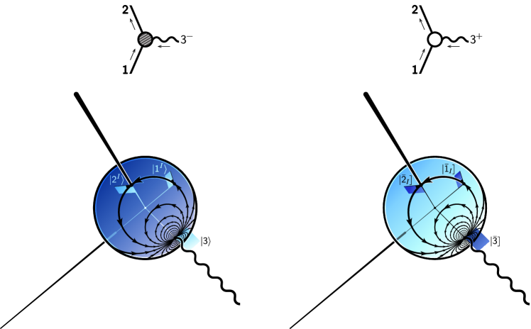
Figure 2: Null rotation on the left and right skies. As a conformal transformation on the celestial sphere, it preserves the angle that the null flag of the spinor being transformed makes with the circular flow lines. This provides a geometrical way of seeing $\langle{\mathsf{3}}{\mathsf{2}}^{I}\rangle=\langle{\mathsf{3}}{\mathsf{1}}^{I}\rangle$ or $[{\bar{\mathsf{2}}}_{I}{\bar{\mathsf{3}}}]=[{\bar{\mathsf{1}}}_{I}{\bar{\mathsf{3}}}]$ [89].

The parameter $\vartheta$ controls the ratio between the contributions from $\mathit{\Delta}\lambda_{\alpha}{}^{I}$ and $\mathit{\Delta}{\bar{\lambda}}_{I{\dot{\alpha}}}$ that add up to $\mathit{\Delta}p_{\alpha{\dot{\alpha}}}=-{\mathsf{3}}_{\alpha}{\bar{\mathsf{3}}}_{\dot{\alpha}}$. As depicted in the left side of Figure 2, the equation $|{\mathsf{2}}^{I}\rangle=|{\mathsf{1}}^{I}\rangle+{t\hskip 1.00006pt|{\mathsf{3}}\rangle\langle{\mathsf{3}}{\mathsf{1}}^{I}\rangle}$ has a geometric interpretation as a null rotation [89] on the celestial sphere that takes the flagpole direction of the spinor $|{\mathsf{3}}\rangle$ as the fixed point. Then (93) is a complexified Lorentz transformation that null rotates the celestial spheres of the right-handed and left-handed spinors differently.

In analogy with the MHV kinematics [174], we consider the following two extreme cases.

$$\,\,\,\leftrightarrow\,\,\,\left\{{\begin{array}[]{rl}|{\mathsf{2}}^{I}\rangle&{}=|{\mathsf{1}}^{I}\rangle\phantom{{}+(x/m)\hskip 1.00006pt|{\mathsf{3}}\rangle\langle{\mathsf{3}}{\mathsf{1}}^{I}\rangle}\\ {\kern-0.37003pt\leavevmode\hbox{$\vbox{\hbox{\resizebox{}{}{\scalebox{0.99}[0.99]{{\leavevmode\hbox{\set@color{${\lfloor\hbox to0.0pt{\hss\reflectbox{\rotatebox[origin={c}]{180.0}{$\lfloor$}}}}$}}}}}}}$}\kern-0.39993pt}{\bar{\mathsf{2}}}_{I}|&{}={\kern-0.37003pt\leavevmode\hbox{$\vbox{\hbox{\resizebox{}{}{\scalebox{0.99}[0.99]{{\leavevmode\hbox{\set@color{${\lfloor\hbox to0.0pt{\hss\reflectbox{\rotatebox[origin={c}]{180.0}{$\lfloor$}}}}$}}}}}}}$}\kern-0.39993pt}{\bar{\mathsf{1}}}_{I}|+(1/mx)\hskip 1.00006pt{\kern-0.37003pt\leavevmode\hbox{$\vbox{\hbox{\resizebox{}{}{\scalebox{0.99}[0.99]{{\leavevmode\hbox{\set@color{${\lfloor\hbox to0.0pt{\hss\reflectbox{\rotatebox[origin={c}]{180.0}{$\lfloor$}}}}$}}}}}}}$}\kern-0.39993pt}{\bar{\mathsf{1}}}_{I}{\bar{\mathsf{3}}}{\kern-0.39993pt\leavevmode\hbox{$\vbox{\hbox{\resizebox{}{}{\scalebox{0.99}[0.99]{{\leavevmode\hbox{\set@color{${\hbox to0.0pt{\reflectbox{\rotatebox[origin={c}]{180.0}{$\rfloor$}}\hss}\rfloor}$}}}}}}}$}\kern-0.37003pt}{\kern-0.37003pt\leavevmode\hbox{$\vbox{\hbox{\resizebox{}{}{\scalebox{0.99}[0.99]{{\leavevmode\hbox{\set@color{${\lfloor\hbox to0.0pt{\hss\reflectbox{\rotatebox[origin={c}]{180.0}{$\lfloor$}}}}$}}}}}}}$}\kern-0.39993pt}{\bar{\mathsf{3}}}|\end{array}}\right.$$ (94c)

$$\,\,\,\leftrightarrow\,\,\,\left\{{\begin{array}[]{rl}|{\mathsf{2}}^{I}\rangle&{}=|{\mathsf{1}}^{I}\rangle+(x/m)\hskip 1.00006pt|{\mathsf{3}}\rangle\langle{\mathsf{3}}{\mathsf{1}}^{I}\rangle\\ {\kern-0.37003pt\leavevmode\hbox{$\vbox{\hbox{\resizebox{}{}{\scalebox{0.99}[0.99]{{\leavevmode\hbox{\set@color{${\lfloor\hbox to0.0pt{\hss\reflectbox{\rotatebox[origin={c}]{180.0}{$\lfloor$}}}}$}}}}}}}$}\kern-0.39993pt}{\bar{\mathsf{2}}}_{I}|&{}={\kern-0.37003pt\leavevmode\hbox{$\vbox{\hbox{\resizebox{}{}{\scalebox{0.99}[0.99]{{\leavevmode\hbox{\set@color{${\lfloor\hbox to0.0pt{\hss\reflectbox{\rotatebox[origin={c}]{180.0}{$\lfloor$}}}}$}}}}}}}$}\kern-0.39993pt}{\bar{\mathsf{1}}}_{I}|\phantom{{}+(1/mx)\hskip 1.00006pt{\kern-0.37003pt\leavevmode\hbox{$\vbox{\hbox{\resizebox{}{}{\scalebox{0.99}[0.99]{{\leavevmode\hbox{\set@color{${\lfloor\hbox to0.0pt{\hss\reflectbox{\rotatebox[origin={c}]{180.0}{$\lfloor$}}}}$}}}}}}}$}\kern-0.39993pt}{\bar{\mathsf{1}}}_{I}{\bar{\mathsf{3}}}{\kern-0.39993pt\leavevmode\hbox{$\vbox{\hbox{\resizebox{}{}{\scalebox{0.99}[0.99]{{\leavevmode\hbox{\set@color{${\hbox to0.0pt{\reflectbox{\rotatebox[origin={c}]{180.0}{$\rfloor$}}\hss}\rfloor}$}}}}}}}$}\kern-0.37003pt}{\kern-0.37003pt\leavevmode\hbox{$\vbox{\hbox{\resizebox{}{}{\scalebox{0.99}[0.99]{{\leavevmode\hbox{\set@color{${\lfloor\hbox to0.0pt{\hss\reflectbox{\rotatebox[origin={c}]{180.0}{$\lfloor$}}}}$}}}}}}}$}\kern-0.39993pt}{\bar{\mathsf{3}}}|}\end{array}}\right.$$ (94f)

These complexified kinematics naturally arise from the minimally coupled heavenly equations of motion; for instance, (56) parallel-transports $\lambda_{\alpha}{}^{I}$ while preserving ${\bar{\Delta}}$. They are associated with zig-zag vector fields (as operators on the $(\lambda,{\bar{\lambda}})$ Lagrange submanifold, say) as the following:

$$\includegraphics[scale={1.0},valign={c}]{figs/hkin-.pdf}\,\,\,\sim\,\,\,\includegraphics[valign={c}]{figs/l.pdf}\includegraphics[valign={c}]{figs/v-.pdf}\includegraphics[valign={c}]{figs/xD.pdf}\,,\qquad\quad\includegraphics[scale={1.0},valign={c}]{figs/hkin+.pdf}\,\,\,\sim\,\,\,\includegraphics[valign={c}]{figs/l-b.pdf}\includegraphics[valign={c}]{figs/v+.pdf}\includegraphics[valign={c}]{figs/xD-b.pdf}\,.$$ (95)

Minimal impulse and amplitude

The amplitudes can be conveniently obtained by computing the interaction action for a zeroth-order trajectory in an on-shell plane wave background (cf. Appendix A of [10]). However, to keep pursuing the “symplectic form only” philosophy, we rather relate the zig-zag expansions to amplitudes by computing the impulses. The zig-zag vector field (54) is evaluated for (90) as

$$\begin{split}-\smash{\includegraphics[valign={c}]{figs/l-b.pdf}\includegraphics[valign={c}]{figs/v+.pdf}\includegraphics[valign={c}]{figs/xD-b.pdf}}\,\hskip 1.00006pt&=\,\,\{{\,\,\,\,\,},z^{{\dot{\alpha}}\alpha}\}^{\circ}\,\hskip 1.00006pt(2/\Delta)\hskip 1.00006ptp_{\smash{\alpha{\dot{\beta}}}\vphantom{{\dot{\alpha}}}}\hskip 1.00006pt\phi^{\dot{\beta}}{}_{\dot{\alpha}}(z)\,,\\ &=\,\,\{{\,\,\,\,\,},z^{{\dot{\alpha}}\alpha}\}^{\circ}\,\hskip 1.00006pti\big{(}\hskip 1.00006pt\nu\hskip 1.00006ptp_{\smash{\alpha{\dot{\beta}}}\vphantom{\beta}}{\kern 0.09995pt}{\bar{o}}^{\dot{\beta}}{\bar{o}}_{\smash{{\dot{\alpha}}}\vphantom{\alpha}}\hskip 0.50003pt\big{)}\hskip 1.00006pt{\mathrm{e}}^{-i\hskip 0.35002pt{\bar{o}zo}}/\Delta\,,\\ &=\,\,\{{\,\,\,\,\,},z^{{\dot{\alpha}}\alpha}\}^{\circ}\,\hskip 1.00006pti\big{(}\hskip 1.00006pt\nu\langle\iota|p|{\bar{o}}{\kern-0.39993pt\leavevmode\hbox{$\vbox{\hbox{\resizebox{}{}{\scalebox{0.99}[0.99]{{\leavevmode\hbox{\set@color{${\hbox to0.0pt{\reflectbox{\rotatebox[origin={c}]{180.0}{$\rfloor$}}\hss}\rfloor}$}}}}}}}$}\kern-0.37003pt}\hskip 0.50003pt{\mathrm{e}}^{{\bar{o}}yo}\hskip 1.00006pto_{\alpha}{\bar{o}}_{\dot{\alpha}}-\nu\langle o|p|{\bar{o}}{\kern-0.39993pt\leavevmode\hbox{$\vbox{\hbox{\resizebox{}{}{\scalebox{0.99}[0.99]{{\leavevmode\hbox{\set@color{${\hbox to0.0pt{\reflectbox{\rotatebox[origin={c}]{180.0}{$\rfloor$}}\hss}\rfloor}$}}}}}}}$}\kern-0.37003pt}\hskip 0.50003pt{\mathrm{e}}^{{\bar{o}}yo}\hskip 1.00006pt\iota_{\alpha}{\bar{o}}_{\dot{\alpha}}\hskip 0.50003pt\big{)}\hskip 1.00006pt{\mathrm{e}}^{-i{\bar{o}}xo}/\Delta\,.\end{split}$$ (96)

We have used $\delta_{\alpha}{}^{\beta}=o_{\alpha}\iota^{\beta}-\iota_{\alpha}o^{\beta}$ in the last line. The heavenly “ambitwistor impulse” follows from integrating (LABEL:eq:3vec+1) over time:

$$\mathit{\Delta}Z_{\mathrm{A}}{}^{I}=0\,,\quad\mathit{\Delta}{\bar{Z}}_{I}{}^{\mathrm{A}}=\int_{-\infty}^{+\infty}\frac{d\tau}{-2}\,\Big{\langle}d{\bar{Z}}_{I}{}^{\mathrm{A}},-\smash{\includegraphics[valign={c}]{figs/l-b.pdf}\includegraphics[valign={c}]{figs/v+.pdf}\includegraphics[valign={c}]{figs/xD-b.pdf}}\Big{\rangle}\,.$$ (97)

The recipe to obtain the amplitude is identifying the amount of impulse expected from the particle interpretation (absorption of a single quantum) and then reading off the proportionality factor from $\mathit{\Delta}p_{\alpha{\dot{\alpha}}}$. In the first-order approximation, the integration (97) does nothing other than inducing the delta function $\delta\kern-1.99997pt\makebox[0.0pt][l]{$\bar{}$}\kern 1.99997pt(\langle o|{\mathsf{1}}|{\bar{o}}{\kern-0.39993pt\leavevmode\hbox{$\vbox{\hbox{\resizebox{}{}{\scalebox{0.99}[0.99]{{\leavevmode\hbox{\set@color{${\hbox to0.0pt{\reflectbox{\rotatebox[origin={c}]{180.0}{$\rfloor$}}\hss}\rfloor}$}}}}}}}$}\kern-0.37003pt}\hskip 0.50003pt)$. Thus, we can just directly read off the “amplitude times momentum kick” $(\nu m_{0}x\hskip 1.00006pt{\mathrm{e}}^{{\mathsf{3}}\cdot a})(-{\mathsf{3}}_{\alpha}{\bar{\mathsf{3}}}_{\dot{\alpha}})$ from the bracketed term in the last line of (LABEL:eq:3vec+1) by putting $\langle o|p|{\bar{o}}{\kern-0.39993pt\leavevmode\hbox{$\vbox{\hbox{\resizebox{}{}{\scalebox{0.99}[0.99]{{\leavevmode\hbox{\set@color{${\hbox to0.0pt{\reflectbox{\rotatebox[origin={c}]{180.0}{$\rfloor$}}\hss}\rfloor}$}}}}}}}$}\kern-0.37003pt}=0$ and plugging in the scattering data $p_{\alpha{\dot{\alpha}}}{\,=\,}{\mathsf{1}}_{\alpha{\dot{\alpha}}}$, $y^{{\dot{\alpha}}\alpha}{\,=\,}{{-}a^{{\dot{\alpha}}\alpha}}$. In this sense, the vector field (LABEL:eq:3vec+1) is a “symplectic avatar” of the positive-helicity three-point amplitude. Note that it performs a null rotation on ${\bar{\lambda}}_{I{\dot{\alpha}}}$, $y^{{\dot{\alpha}}\alpha}$:

$$\{{\,\,\,\,\,},z^{{\dot{\alpha}}\alpha}\}^{\circ}\,\hskip 1.00006pti\nu\hskip 1.00006ptp_{\smash{\alpha{\dot{\beta}}}\vphantom{\beta}}{\kern 0.09995pt}{\bar{o}}^{\dot{\beta}}{\bar{o}}_{\smash{{\dot{\alpha}}}\vphantom{\alpha}}\hskip 1.00006pt\frac{{\mathrm{e}}^{-i\hskip 0.35002pt{\bar{o}zo}}}{\Delta}\,=\,\bigg{(}\hskip 0.50003pt{{\bar{\lambda}}_{I{\dot{\beta}}}\hskip 1.00006pt\frac{\partial}{\partial{\bar{\lambda}}_{I{\dot{\alpha}}}}-y^{{\dot{\alpha}}\beta}\left.\frac{\partial}{\partial y^{{\dot{\beta}}\beta}}\right|_{z}\hskip 1.00006pt}\bigg{)}\hskip 1.00006pt\hskip 0.50003pti\nu\hskip 1.00006pt{\bar{o}}^{\dot{\beta}}{\bar{o}}_{\smash{{\dot{\alpha}}}\vphantom{\alpha}}\hskip 1.00006pt\frac{{\mathrm{e}}^{-i\hskip 0.35002pt{\bar{o}zo}}}{\Delta}\,.$$ (98)

The amplitude $\nu m_{0}x\hskip 1.00006pt{\mathrm{e}}^{{\mathsf{3}}\cdot a}$ is precisely the scalar amplitude $e_{h}\hskip 0.50003ptm_{0}x^{h}$ [3] times the minimal exponential spin factor [8, 7] if

$$\nu=e_{h}\hskip 0.50003ptx^{h-1}\,,$$ (99)

where $e_{h}$ collectively denotes the coupling constants of Yang-Mills ($h{\hskip 1.00006pt=\hskip 1.00006pt}1$) and gravity ($h{\hskip 1.00006pt=\hskip 1.00006pt}2$). We revisit this finding later in section 4.1.

Generic impulse and amplitude

For non-minimal couplings, the interaction with the self-dual plane wave alters both $\lambda_{\alpha}{}^{I}$ and ${\bar{\lambda}}_{I{\dot{\alpha}}}$. Consider the maximally non-minimal coupling for an example; the first two “avatar” vector fields (63a)-(63b) contribute to the first-order $\mathit{\Delta}{\bar{\lambda}}_{I{\dot{\alpha}}}$, while (63c)-(63d) contribute to $\mathit{\Delta}\lambda_{\alpha}{}^{I}$. Generalizing, one finds

$$\begin{split}\mathit{\Delta}^{(1)}{\kern-0.37003pt\leavevmode\hbox{$\vbox{\hbox{\resizebox{}{}{\scalebox{0.99}[0.99]{{\leavevmode\hbox{\set@color{${\lfloor\hbox to0.0pt{\hss\reflectbox{\rotatebox[origin={c}]{180.0}{$\lfloor$}}}}$}}}}}}}$}\kern-0.39993pt}{\bar{\lambda}}_{I}|&\hskip 1.00006pt=\,i\Big{(}\hskip 1.00006pt\hskip 0.50003pt\nu m_{0}x\hskip 1.00006pt{\mathrm{e}}^{{\mathsf{3}}\cdot a}\,{\cdot}\,{{}^{0+1}\mathfrak{S}[f^{+}]({\mathsf{3}}{\kern 0.20004pt\cdot\kern 0.20004pt}a)}\hskip 0.50003pt\Big{)}\,\delta\kern-1.99997pt\makebox[0.0pt][l]{$\bar{}$}\kern 1.99997pt(2\hskip 1.00006pt{\mathsf{3}}{\kern 0.20004pt\cdot\kern 0.20004pt}{\mathsf{1}})\,\hskip 1.00006pt{\textstyle\frac{1}{m_{0}x}}{\kern-0.37003pt\leavevmode\hbox{$\vbox{\hbox{\resizebox{}{}{\scalebox{0.99}[0.99]{{\leavevmode\hbox{\set@color{${\lfloor\hbox to0.0pt{\hss\reflectbox{\rotatebox[origin={c}]{180.0}{$\lfloor$}}}}$}}}}}}}$}\kern-0.39993pt}{\bar{\mathsf{1}}}_{I}{\bar{\mathsf{3}}}{\kern-0.39993pt\leavevmode\hbox{$\vbox{\hbox{\resizebox{}{}{\scalebox{0.99}[0.99]{{\leavevmode\hbox{\set@color{${\hbox to0.0pt{\reflectbox{\rotatebox[origin={c}]{180.0}{$\rfloor$}}\hss}\rfloor}$}}}}}}}$}\kern-0.37003pt}{\kern-0.37003pt\leavevmode\hbox{$\vbox{\hbox{\resizebox{}{}{\scalebox{0.99}[0.99]{{\leavevmode\hbox{\set@color{${\lfloor\hbox to0.0pt{\hss\reflectbox{\rotatebox[origin={c}]{180.0}{$\lfloor$}}}}$}}}}}}}$}\kern-0.39993pt}{\bar{\mathsf{3}}}|\,,\\ \mathit{\Delta}^{(1)}|\lambda^{I}\rangle&\hskip 1.00006pt=\,i\Big{(}\hskip 1.00006pt\hskip 0.50003pt\nu m_{0}x\hskip 1.00006pt{\mathrm{e}}^{{\mathsf{3}}\cdot a}\,{\cdot}\,{{}^{1+2}\mathfrak{S}[f^{+}]({\mathsf{3}}{\kern 0.20004pt\cdot\kern 0.20004pt}a)}\hskip 0.50003pt\Big{)}\,\delta\kern-1.99997pt\makebox[0.0pt][l]{$\bar{}$}\kern 1.99997pt(2\hskip 1.00006pt{\mathsf{3}}{\kern 0.20004pt\cdot\kern 0.20004pt}{\mathsf{1}})\,{\textstyle\frac{x}{m_{0}}}\hskip 0.50003pt|{\mathsf{3}}\rangle\langle{\mathsf{3}}{\mathsf{1}}^{I}\rangle\,,\end{split}$$ (100)

while replacing $iy^{m}\partial/\partial x^{m}$ with $i(-a^{m})(i{\mathsf{3}}_{m})={\mathsf{3}}{\hskip 1.00006pt\cdot\hskip 1.00006pt}a$. The $x$-factor is defined on the support of $\delta\kern-1.99997pt\makebox[0.0pt][l]{$\bar{}$}\kern 1.99997pt(2\hskip 1.00006pt{\mathsf{3}}{\hskip 1.00006pt\cdot\hskip 1.00006pt}{\mathsf{1}})$. Adding up these two and using the identity ${{}^{0}\mathfrak{S}[f](\xi)}+2\hskip 1.00006pt{{}^{1}\mathfrak{S}[f](\xi)}+{{}^{2}\mathfrak{S}[f](\xi)}=f(\xi)$, we find the momentum impulse

$$\mathit{\Delta}^{(1)}p_{\alpha{\dot{\alpha}}}=i\Big{(}\hskip 1.00006pt\hskip 0.50003pt\nu m_{0}x\hskip 1.00006pt{\mathrm{e}}^{{\mathsf{3}}\cdot a}\,{\cdot}\,f^{+}({\mathsf{3}}{\kern 0.20004pt\cdot\kern 0.20004pt}a)\hskip 0.50003pt\Big{)}\,\delta\kern-1.99997pt\makebox[0.0pt][l]{$\bar{}$}\kern 1.99997pt(2\hskip 1.00006pt{\mathsf{3}}{\kern 0.20004pt\cdot\kern 0.20004pt}{\mathsf{1}})\,(-{\mathsf{3}}_{\alpha}{\bar{\mathsf{3}}}_{\dot{\alpha}})\,.$$ (101)

For concreteness, we also spell out the negative-helicity counterparts. A positive-frequency field quantum carrying negative helicity is described by ${\bar{\phi}}_{\alpha\beta}({\bar{z}})=(i\nu/2)\hskip 1.00006pto_{\alpha}o_{\beta}\hskip 1.00006pt{\mathrm{e}}^{-i{\bar{o}}{\bar{z}}o}$ (note that it is not the straightforward complex conjugate of (90)). We find

$$\begin{split}\mathit{\Delta}^{(1)}{\kern-0.37003pt\leavevmode\hbox{$\vbox{\hbox{\resizebox{}{}{\scalebox{0.99}[0.99]{{\leavevmode\hbox{\set@color{${\lfloor\hbox to0.0pt{\hss\reflectbox{\rotatebox[origin={c}]{180.0}{$\lfloor$}}}}$}}}}}}}$}\kern-0.39993pt}{\bar{\lambda}}_{I}|&\hskip 1.00006pt=\,i\Big{(}\hskip 1.00006pt\hskip 0.50003pt\nu m_{0}x^{-1}\hskip 1.00006pt{\mathrm{e}}^{-{\mathsf{3}}{\hskip 0.70004pt\cdot\hskip 0.70004pt}a}\,{\cdot}\,{{}^{1+2}\mathfrak{S}[f^{-}](-{\mathsf{3}}{\kern 0.20004pt\cdot\kern 0.20004pt}a)}\hskip 0.50003pt\Big{)}\,\delta\kern-1.99997pt\makebox[0.0pt][l]{$\bar{}$}\kern 1.99997pt(2\hskip 1.00006pt{\mathsf{3}}{\kern 0.20004pt\cdot\kern 0.20004pt}{\mathsf{1}})\,\hskip 1.00006pt{\textstyle\frac{1}{m_{0}x}}{\kern-0.37003pt\leavevmode\hbox{$\vbox{\hbox{\resizebox{}{}{\scalebox{0.99}[0.99]{{\leavevmode\hbox{\set@color{${\lfloor\hbox to0.0pt{\hss\reflectbox{\rotatebox[origin={c}]{180.0}{$\lfloor$}}}}$}}}}}}}$}\kern-0.39993pt}{\bar{\mathsf{1}}}_{I}{\bar{\mathsf{3}}}{\kern-0.39993pt\leavevmode\hbox{$\vbox{\hbox{\resizebox{}{}{\scalebox{0.99}[0.99]{{\leavevmode\hbox{\set@color{${\hbox to0.0pt{\reflectbox{\rotatebox[origin={c}]{180.0}{$\rfloor$}}\hss}\rfloor}$}}}}}}}$}\kern-0.37003pt}{\kern-0.37003pt\leavevmode\hbox{$\vbox{\hbox{\resizebox{}{}{\scalebox{0.99}[0.99]{{\leavevmode\hbox{\set@color{${\lfloor\hbox to0.0pt{\hss\reflectbox{\rotatebox[origin={c}]{180.0}{$\lfloor$}}}}$}}}}}}}$}\kern-0.39993pt}{\bar{\mathsf{3}}}|\,,\\ \mathit{\Delta}^{(1)}|\lambda^{I}\rangle&\hskip 1.00006pt=\,i\Big{(}\hskip 1.00006pt\hskip 0.50003pt\nu m_{0}x^{-1}\hskip 1.00006pt{\mathrm{e}}^{-{\mathsf{3}}{\hskip 0.70004pt\cdot\hskip 0.70004pt}a}\,{\cdot}\,{{}^{0+1}\mathfrak{S}[f^{-}](-{\mathsf{3}}{\kern 0.20004pt\cdot\kern 0.20004pt}a)}\hskip 0.50003pt\Big{)}\,\delta\kern-1.99997pt\makebox[0.0pt][l]{$\bar{}$}\kern 1.99997pt(2\hskip 1.00006pt{\mathsf{3}}{\kern 0.20004pt\cdot\kern 0.20004pt}{\mathsf{1}})\,{\textstyle\frac{x}{m_{0}}}\hskip 0.50003pt|{\mathsf{3}}\rangle\langle{\mathsf{3}}{\mathsf{1}}^{I}\rangle\,,\end{split}$$ (102)

$$\mathit{\Delta}^{(1)}p_{\alpha{\dot{\alpha}}} \hskip 1.00006pt=\,i\Big{(}\hskip 1.00006pt\hskip 0.50003pt\nu m_{0}x^{-1}\hskip 1.00006pt{\mathrm{e}}^{-{\mathsf{3}}{\hskip 0.70004pt\cdot\hskip 0.70004pt}a}\,{\cdot}\,f^{-}(-{\mathsf{3}}{\kern 0.20004pt\cdot\kern 0.20004pt}a)\hskip 0.50003pt\Big{)}\,\delta\kern-1.99997pt\makebox[0.0pt][l]{$\bar{}$}\kern 1.99997pt(2\hskip 1.00006pt{\mathsf{3}}{\kern 0.20004pt\cdot\kern 0.20004pt}{\mathsf{1}})\,(-{\mathsf{3}}_{\alpha}{\bar{\mathsf{3}}}_{\dot{\alpha}})\,.$$ (103)

The helicity flip is effectively implemented by the sign change of the pseudovector $a^{m}$.

To summarize, we have obtained the minimal and non-minimal amplitudes as follows:

$${\mathcal{M}}^{\pm h}({\mathsf{1}},a;{\mathsf{3}})=e_{h}\hskip 0.50003ptm_{0}x^{h}\hskip 1.00006pt\hskip 0.50003pt{\mathrm{e}}^{\pm{\mathsf{3}}\cdot a}\,,\quad{\mathcal{M}}^{\pm h}[f^{\pm}]({\mathsf{1}},a;{\mathsf{3}})={\mathcal{M}}^{\pm h}({\mathsf{1}},a;{\mathsf{3}})\,{\cdot}\,f^{\pm}(\pm{\mathsf{3}}{\kern 0.20004pt\cdot\kern 0.20004pt}a)\,.$$ (104)

For example, the “exponential” arbitrary-$g$ coupling (70) leads to

$$\begin{split}f^{\pm}(\xi)={\mathrm{e}}^{(g/2-1)\xi}&{\quad\implies\quad}{\mathcal{M}}^{\pm h}[f^{\pm}]({\mathsf{1}},a;{\mathsf{3}})={\mathcal{M}}^{\pm h}({\mathsf{1}},a;{\mathsf{3}})\,{\cdot}\,{\mathrm{e}}^{\pm(g/2-1)\hskip 0.35002pt{\mathsf{3}}{\kern 0.14003pt\cdot\kern 0.14003pt}a}\,.\end{split}$$ (105)

Moreover, we also derived classical complexified kinematics corresponding to the non-minimal amplitudes. Peeling off the amplitudes ${\mathcal{M}}^{\pm h}[f^{\pm}]({\mathsf{1}},a;{\mathsf{3}})$ from the impulses (100) and (102), we find that the “asymmetry parameter” $\vartheta$ of (93) is given by

$$\pm\vartheta\,=\,{\textstyle\frac{1}{2}}\hskip 1.00006pt{{}^{0-2}\mathfrak{S}[f^{\pm}](\pm{\mathsf{3}}{\kern 0.20004pt\cdot\kern 0.20004pt}a)}\hskip 1.00006pt:=\hskip 1.00006pt{\textstyle\frac{1}{2}}\big{(}\hskip 1.00006pt{{{}^{0}\mathfrak{S}[f^{\pm}](\pm{\mathsf{3}}{\kern 0.20004pt\cdot\kern 0.20004pt}a)}-{{}^{2}\mathfrak{S}[f^{\pm}](\pm{\mathsf{3}}{\kern 0.20004pt\cdot\kern 0.20004pt}a)}}\big{)}$$ (106)

for positive-helicity and negative-helicity amplitudes, respectively. It is easy to see that (70) leads to $\vartheta=g$. Especially, $g=0$ leads to the real kinematics (92).

Matching with definite-spin amplitudes

Finally, we explicate the connection with the discrete definite-spin amplitudes. Previous studies [9, 2, 8, 11, 21, 10] have established a dictionary between the Wilson coefficients $C^{\pm}_{\ell}$ and the coupling constants $g^{\pm}_{\ell}$ appearing in the generic three-point amplitude [3]:

$$\mathcal{A}^{+h}_{(2s)}[g^{+}]({\mathsf{2}}{\leftarrow}{\mathsf{1}};{\mathsf{3}}) \hskip 1.00006pt=\hskip 1.00006pte_{h}\hskip 0.50003ptm_{0}x^{h}\hskip 1.00006pt\sum_{\ell=0}^{2s}\hskip 1.00006ptg^{+}_{\ell}\hskip 1.00006pt\langle{\mathsf{2}}^{-1}{\mathsf{1}}\rangle^{\kern-0.35002pt\odot(2s-\ell)}{\hskip 1.00006pt\odot}\left(\frac{x}{m_{0}/\hbar}\langle{\mathsf{2}}^{-1}{\mathsf{3}}\rangle\langle{\mathsf{3}}{\mathsf{1}}\rangle\right)^{\kern-1.92496pt\odot\ell}\,,$$ (107a)

$$\mathcal{A}^{-h}_{(2s)}[g^{-}]({\mathsf{2}}{\leftarrow}{\mathsf{1}};{\mathsf{3}}) \hskip 1.00006pt=\hskip 1.00006pte_{h}\hskip 0.50003ptm_{0}x^{h}\hskip 1.00006pt\sum_{\ell=0}^{2s}\hskip 1.00006ptg^{-}_{\ell}\hskip 1.00006pt{\kern-0.37003pt\leavevmode\hbox{$\vbox{\hbox{\resizebox{}{}{\scalebox{0.99}[0.99]{{\leavevmode\hbox{\set@color{${\lfloor\hbox to0.0pt{\hss\reflectbox{\rotatebox[origin={c}]{180.0}{$\lfloor$}}}}$}}}}}}}$}\kern-0.39993pt}{\bar{\mathsf{2}}}{\bar{\mathsf{1}}}^{-1}{\kern-0.39993pt\leavevmode\hbox{$\vbox{\hbox{\resizebox{}{}{\scalebox{0.99}[0.99]{{\leavevmode\hbox{\set@color{${\hbox to0.0pt{\reflectbox{\rotatebox[origin={c}]{180.0}{$\rfloor$}}\hss}\rfloor}$}}}}}}}$}\kern-0.37003pt}^{\kern-0.35002pt\odot(2s-\ell)}{\hskip 1.00006pt\odot}\left(\frac{1}{(m_{0}/\hbar)x}{\kern-0.37003pt\leavevmode\hbox{$\vbox{\hbox{\resizebox{}{}{\scalebox{0.99}[0.99]{{\leavevmode\hbox{\set@color{${\lfloor\hbox to0.0pt{\hss\reflectbox{\rotatebox[origin={c}]{180.0}{$\lfloor$}}}}$}}}}}}}$}\kern-0.39993pt}{\bar{\mathsf{2}}}{\bar{\mathsf{3}}}{\kern-0.39993pt\leavevmode\hbox{$\vbox{\hbox{\resizebox{}{}{\scalebox{0.99}[0.99]{{\leavevmode\hbox{\set@color{${\hbox to0.0pt{\reflectbox{\rotatebox[origin={c}]{180.0}{$\rfloor$}}\hss}\rfloor}$}}}}}}}$}\kern-0.37003pt}{\kern-0.37003pt\leavevmode\hbox{$\vbox{\hbox{\resizebox{}{}{\scalebox{0.99}[0.99]{{\leavevmode\hbox{\set@color{${\lfloor\hbox to0.0pt{\hss\reflectbox{\rotatebox[origin={c}]{180.0}{$\lfloor$}}}}$}}}}}}}$}\kern-0.39993pt}{\bar{\mathsf{3}}}{\bar{\mathsf{1}}}^{-1}{\kern-0.39993pt\leavevmode\hbox{$\vbox{\hbox{\resizebox{}{}{\scalebox{0.99}[0.99]{{\leavevmode\hbox{\set@color{${\hbox to0.0pt{\reflectbox{\rotatebox[origin={c}]{180.0}{$\rfloor$}}\hss}\rfloor}$}}}}}}}$}\kern-0.37003pt}\right)^{\kern-1.92496pt\odot\ell}\,.$$ (107b)

We have temporarily restored $\hbar$. We restrict our attention to the diagonal (equal-mass and equal-spin) sector. As a result of the matching, one finds

$${\mathrm{e}}^{\xi}{\,\cdot\,}f^{\pm}(\xi)\hskip 1.00006pt=\hskip 1.00006ptC^{\pm}(\xi)\hskip 1.00006pt=\hskip 1.00006pt{\mathrm{e}}^{\xi}{\,\cdot\,}\hskip 0.50003ptg^{\pm}(-\xi/|\vec{W}|){\quad\implies\quad}f^{\pm}(\xi)\hskip 1.00006pt=\hskip 1.00006ptg^{\pm}(-\xi/|\vec{W}|)\,,$$ (108)

where the generating function describing the classical limit of $g^{\pm}_{\ell}$ is defined as

$$g^{\pm}(\xi):=\lim_{\hbar\to 0}\sum_{\ell=0}^{\infty}g^{\pm}_{\ell}(\hbar\xi)^{\ell}\,.$$ (109)

Notice that Wilson coefficients on complex worldlines, $f^{\pm}_{\ell}$, are more straightforwardly related to the coupling constants $g^{\pm}_{\ell}$. As a pedagogical demonstration, we re-derive (108) in appendix B without resorting to the “real-based” Wilson coefficients $C^{\pm}_{\ell}$. We briefly discuss how the spin coherent states are implemented in the spherical top framework and then reproduce [10]’s matching calculation with our notations and conventions. We also observe that using the complexified kinematics (94c)-(94f), rather than the real kinematics (92), provides a “shortcut” for the calculations.

4 Scattering of $\sqrt{\text{Kerr\hskip 0.50003pt}}$ and Kerr in Heavenly Plane Waves

In the previous section, we have studied “universal” implications of relating chirality and holomorphy on the linear-order perturbative physics, leaving $\phi$ unspecified. In this section, we finally specialize $\phi$ to Yang-Mills and gravity. Still, we continue pursuing a “bottom-up” approach: we reverse engineer the $\sqrt{\text{Kerr\hskip 0.50003pt}}$ and Kerr actions in heavenly backgrounds from the matching (99) between the minimal amplitude $e_{h}\hskip 0.50003ptm_{0}x^{h}\hskip 1.00006pt{\mathrm{e}}^{{\mathsf{3}}\cdot a}$ and the plane wave ansatz (90), without having a top-down picture. Furthermore, we also exactly solve the classical dynamics of $\sqrt{\text{Kerr\hskip 0.50003pt}}$ and Kerr in self-dual plane-wave backgrounds of arbitrarily (non-perturbatively) large magnitudes and re-derive their impulses as exact quantities, thus examining the validity of the results of Section 3.3 for $\sqrt{\text{Kerr\hskip 0.50003pt}}$ and Kerr.

4.1 Corrections from symplectivity

Heavenly plane-wave symplectic perturbations

The classical-spin amplitudes of $\sqrt{\text{Kerr\hskip 0.50003pt}}$ and Kerr particles are given as [7, 10]

$${\mathcal{M}}^{+h}({\mathsf{1}},a;{\mathsf{3}})=e_{h}\hskip 0.50003ptmx^{h}\hskip 1.00006pt{\mathrm{e}}^{{\mathsf{3}}\cdot a}\,,\quad(e_{1},e_{2})=(\sqrt{2}g\hskip 1.00006ptq_{a}c^{a},m{/}{M_{\text{Pl}}})\,,$$ (110)

where $g$ and $M_{\text{Pl}}:=(8\pi G)^{-1/2}$ are the Yang-Mills coupling constant and the Planck mass, respectively. $q_{a}$ denotes the non-abelian color charge of the $\sqrt{\text{Kerr\hskip 0.50003pt}}$ particle, and $c^{a}$ denotes the color “polarization.” As already pointed out in (99), the amplitude $\nu mx\hskip 0.50003pt{\mathrm{e}}^{{\mathsf{3}}\cdot a}$ boils down to (110) if $\nu=e_{h}\hskip 0.50003ptx^{h-1}$ on the support of $\delta\kern-1.99997pt\makebox[0.0pt][l]{$\bar{}$}\kern 1.99997pt(2\hskip 1.00006pt{\mathsf{3}}{\hskip 1.00006pt\cdot\hskip 1.00006pt}{\mathsf{1}})$. A natural guess is

$$\begin{split}\text{{\text{$\sqrt{\text{Kerr\hskip 0.50003pt}}$}}}:\quad\nu=\sqrt{2}g\hskip 1.00006ptq_{a}c^{a}\,,\qquad\text{Kerr}:\quad\nu={M_{\text{Pl}}}^{-1}(-\iota^{\alpha}p_{\alpha{\dot{\alpha}}}{\bar{o}}^{\dot{\alpha}})\,.\end{split}$$ (111)

Accordingly, we can deduce that the $\sqrt{\text{Kerr\hskip 0.50003pt}}$ and Kerr particles have the following symplectic perturbations in the background (90):

$$\text{{\text{$\sqrt{\text{Kerr\hskip 0.50003pt}}$}}}:\quad\omega^{\prime+} =q_{a}\hskip 1.00006pt\frac{ig\hskip 1.00006ptc^{a}}{\sqrt{2}}\hskip 1.00006pt{\bar{o}}_{\dot{\alpha}}\hskip 0.50003pt{\bar{o}}_{\dot{\beta}}\hskip 1.00006pt(dz{\hskip 1.00006pt{\wedge}\,}dz)^{{\dot{\alpha}}{\dot{\beta}}}\hskip 1.00006pt{\mathrm{e}}^{-i\hskip 0.35002pt{\bar{o}zo}}+(\cdots)\,,$$ (112a)

$$\text{Kerr}:\quad\omega^{\prime+} =p_{{\gamma}{\dot{{\gamma}}}}\hskip 1.00006pt\frac{-i\hskip 0.50003pt{\bar{o}}^{\dot{{\gamma}}}\iota^{\gamma}}{2{M_{\text{Pl}}}}\hskip 1.00006pt{\bar{o}}_{\dot{\alpha}}\hskip 0.50003pt{\bar{o}}_{\dot{\beta}}\hskip 1.00006pt(dz{\hskip 1.00006pt{\wedge}\,}dz)^{{\dot{\alpha}}{\dot{\beta}}}\hskip 1.00006pt{\mathrm{e}}^{-i\hskip 0.35002pt{\bar{o}zo}}+(\cdots)\,.$$ (112b)

We have denoted $(dz{\hskip 1.00006pt{\wedge}\,}dz)^{{\dot{\alpha}}{\dot{\beta}}}:=\epsilon_{\alpha\beta}({d{z}^{{\dot{\alpha}}\alpha}\wedge d{z}^{{\dot{\beta}}\beta}})$.

Closure condition

The astute reader may have noticed that, while we have worked as if $\nu$ is a constant in previous sections, $q_{a}c^{a}$ and $(-\iota^{\alpha}p_{\alpha{\dot{\alpha}}}{\bar{o}}^{\dot{\alpha}})$ are actually not. Instead, they turn out to be constants of motion: consider how $d\nu{\hskip 1.00006pt{\wedge}\,}{\kern-0.37003pt\leavevmode\hbox{$\vbox{\hbox{\resizebox{}{}{\scalebox{0.99}[0.99]{{\leavevmode\hbox{\set@color{${\lfloor\hbox to0.0pt{\hss\reflectbox{\rotatebox[origin={c}]{180.0}{$\lfloor$}}}}$}}}}}}}$}\kern-0.39993pt}{\bar{o}}|dz|\iota\rangle\hskip 1.00006pt{\mathrm{e}}^{-i\hskip 0.35002pt{\bar{o}zo}}$ contributes to the zig-zag expansion of $\{\nu,{\bar{\Delta}}\}$. But still, they are not constants “off-shell,” so additional non-$dz{\hskip 1.00006pt{\wedge}\,}dz$ type terms are needed for the closure $d\omega^{\prime+}=0$ as indicated already as ellipses in (112). Noting that the auxiliary spinor $\iota_{\alpha}$ can be traded off with derivatives as

$$\begin{split}i\hskip 0.50003pt\partial_{\beta{\dot{\beta}}}\big{(}{\bar{o}}_{\dot{\alpha}}\hskip 0.50003pt\iota^{\beta}\hskip 1.00006pt{\mathrm{e}}^{-i\hskip 0.35002pt{\bar{o}zo}}\big{)}&={\bar{o}}_{\dot{\alpha}}\hskip 0.50003pt{\bar{o}}_{\dot{\beta}}\hskip 1.00006pt{\mathrm{e}}^{-i\hskip 0.35002pt{\bar{o}zo}}\,,\\ i\hskip 0.50003pt\partial_{{\gamma}{\dot{{\gamma}}}}\big{(}i\hskip 0.50003pt\partial_{{\delta}{\dot{{\delta}}}}\big{(}{\bar{o}}_{\dot{\alpha}}\hskip 0.50003pt{\bar{o}}_{\dot{\beta}}\hskip 0.50003pt\iota^{\gamma}\hskip 0.50003pt\iota^{\delta}\hskip 1.00006pt{\mathrm{e}}^{-i\hskip 0.35002pt{\bar{o}zo}}\big{)}\big{)}&=i\hskip 0.50003pt\partial_{{\delta}{\dot{{\delta}}}}\big{(}{\bar{o}}_{\dot{\alpha}}\hskip 0.50003pt{\bar{o}}_{\dot{\beta}}\hskip 0.50003pt{\bar{o}}_{\dot{{\gamma}}}\hskip 0.50003pt\iota^{\delta}\hskip 1.00006pt{\mathrm{e}}^{-i\hskip 0.35002pt{\bar{o}zo}}\big{)}={\bar{o}}_{\dot{\alpha}}\hskip 0.50003pt{\bar{o}}_{\dot{\beta}}\hskip 0.50003pt{\bar{o}}_{\dot{{\gamma}}}\hskip 0.50003pt{\bar{o}}_{\dot{{\delta}}}\hskip 1.00006pt{\mathrm{e}}^{-i\hskip 0.35002pt{\bar{o}zo}}\,,\end{split}$$ (113)

we can complete (112a)-(112b) as (notice a double copy structure)

$$\text{{\text{$\sqrt{\text{Kerr\hskip 0.50003pt}}$}}}:\quad\omega^{\prime+} =d\Big{(}\hskip 1.00006ptg\hskip 1.00006ptq_{a}c^{a}(\sqrt{2}\hskip 1.00006pt\iota_{\beta}\hskip 0.50003pt{\bar{o}}_{\smash{{\dot{\beta}}}\vphantom{\beta}})\hskip 1.00006ptdz^{{\dot{\beta}}\beta}\hskip 1.00006pt{\mathrm{e}}^{-i\hskip 0.35002pt{\bar{o}zo}}\hskip 0.50003pt\Big{)}\,,$$ (114a)

$$\text{Kerr}:\quad\omega^{\prime+} =d\Big{(}\hskip 0.50003pt{\textstyle-\frac{1}{2M_{\text{Pl}}}}\hskip 1.00006ptp_{\alpha{\dot{\alpha}}}(\sqrt{2}\hskip 1.00006pt\iota^{\alpha}\hskip 0.50003pt{\bar{o}}^{\dot{\alpha}})(\sqrt{2}\hskip 1.00006pt\iota_{\beta}\hskip 0.50003pt{\bar{o}}_{\smash{{\dot{\beta}}}\vphantom{\beta}})\hskip 1.00006ptdz^{{\dot{\beta}}\beta}\hskip 1.00006pt{\mathrm{e}}^{-i\hskip 0.35002pt{\bar{o}zo}}\hskip 0.50003pt\Big{)}\,.$$ (114b)

We see that the additional terms have the forms $dq{\hskip 1.00006pt{\wedge}\,}dz$ and $dp{\hskip 1.00006pt{\wedge}\,}dz$, respectively. Both are admittable in the standard of (27).

Thankfully, since $\{q_{a},\Delta\}^{\circ}=\{q_{a},{\bar{\Delta}}\}^{\circ}=0$ and $\{p_{\alpha{\dot{\alpha}}},\Delta\}^{\circ}=\{p_{\alpha{\dot{\alpha}}},{\bar{\Delta}}\}^{\circ}=0$, these non-spin-space-time “correction” terms do not spoil the “zig-zag” logic of section 3 at all: the $\lambda_{\alpha}{}^{I}$, ${\bar{\lambda}}_{I{\dot{\alpha}}}$, $y^{{\dot{\alpha}}\alpha}$ impulses and the resulting amplitudes remain intact. The only change in the equation of motion is that a “gauge drift” term gets added to the time evolution vector field, contributing to $\dot{q}_{a}$ or $\dot{x}^{{\dot{\alpha}}\alpha}$:

$$\{{\,\,\,\,\,},q_{a}\}^{\circ}\hskip 1.00006pt=\hskip 1.00006pt-q_{c}\hskip 1.00006ptf^{c}{}_{ab}\,\frac{\partial}{\partial q_{b}}\,,\quad\{{\,\,\,\,\,},p_{\alpha{\dot{\alpha}}}\}^{\circ}\hskip 1.00006pt=\hskip 1.00006pt\frac{\partial}{\partial x^{{\dot{\alpha}}\alpha}}\,.$$ (115)

Generic heavenly symplectic perturbations

The sequences (113) reflect the spin-1 and spin-2 nature of Yang-Mills and gravity. Identifying the fully gauge-invariant ${\bar{o}}_{\dot{\alpha}}\hskip 0.50003pt{\bar{o}}_{\dot{\beta}}$ as the self-dual Yang-Mills field strength, its anti-derivative $\iota_{\alpha}\hskip 0.50003pt{\bar{o}}_{\dot{\alpha}}$ is the gauge connection; identifying ${\bar{o}}_{\dot{\alpha}}\hskip 0.50003pt{\bar{o}}_{\dot{\beta}}\hskip 0.50003pt{\bar{o}}_{\dot{{\gamma}}}\hskip 0.50003pt{\bar{o}}_{\dot{{\delta}}}$ as the self-dual Weyl tensor, the two anti-derivatives are the self-dual metric (tetrad) perturbation and spin connection. Indeed, as elaborated in the appendix of [83], the plane-wave gauge fields are given in the lightcone gauge as

$$\begin{split}A^{a}(z)=\sqrt{2}g\hskip 1.00006pt\hskip 0.50003ptc^{a}\hskip 0.50003pt\iota_{\beta}\hskip 0.50003pt{\bar{o}}_{\smash{{\dot{\beta}}}\vphantom{\beta}}\hskip 1.00006ptdz^{{\dot{\beta}}\beta}\hskip 1.00006pt{\mathrm{e}}^{-i\hskip 0.35002pt{\bar{o}zo}}&\,,\quad\textstyle F^{a}(z)=\frac{ig}{\sqrt{2}}\hskip 1.00006pt\hskip 0.50003ptc^{a}\hskip 0.50003pt{\bar{o}}_{\dot{\alpha}}\hskip 0.50003pt{\bar{o}}_{\dot{\beta}}\hskip 0.12497pt(dz{\hskip 1.00006pt{\wedge}\,}dz)^{{\dot{\alpha}}{\dot{\beta}}}\hskip 1.00006pt{\mathrm{e}}^{-i\hskip 0.35002pt{\bar{o}zo}}\,;\\ h^{{\dot{{\gamma}}}{\gamma}}(z)\textstyle={\frac{-1}{{M_{\text{Pl}}}}}\hskip 1.00006pt{\bar{o}}^{\dot{{\gamma}}}\iota^{\gamma}\hskip 0.24994pt\iota_{\beta}\hskip 0.50003pt{\bar{o}}_{\smash{{\dot{\beta}}}\vphantom{\beta}}\hskip 1.00006ptdz^{{\dot{\beta}}\beta}\hskip 1.00006pt{\mathrm{e}}^{-i\hskip 0.35002pt{\bar{o}zo}}&\,,\quad dh^{{\dot{{\gamma}}}{\gamma}}(z)\textstyle={\frac{-i}{2{M_{\text{Pl}}}}}\hskip 1.00006pt{\bar{o}}^{\dot{{\gamma}}}\iota^{\gamma}\hskip 0.50003pt{\bar{o}}_{\dot{\alpha}}\hskip 0.50003pt{\bar{o}}_{\dot{\beta}}\hskip 0.12497pt(dz{\hskip 1.00006pt{\wedge}\,}dz)^{{\dot{\alpha}}{\dot{\beta}}}\hskip 1.00006pt{\mathrm{e}}^{-i\hskip 0.35002pt{\bar{o}zo}}\,.\end{split}$$ (116)

Hence, we can propose that (114a)-(114b) generalize to arbitrary heavenly geometries as

$$\text{{\text{$\sqrt{\text{Kerr\hskip 0.50003pt}}$}}}:\quad\omega^{\prime+} =d\big{(}\hskip 0.50003ptq_{a}A^{a}(z)\big{)} =dq_{a}{\hskip 1.00006pt{\wedge}\,}A^{a}(z)+q_{a}dA^{a}(z)\,,$$ (117a)

$$\text{Kerr}:\quad\omega^{\prime+} =d\big{(}\hskip 0.50003ptp_{\alpha{\dot{\alpha}}}h^{{\dot{\alpha}}\alpha}(z)\big{)} =dp_{\alpha{\dot{\alpha}}}{\hskip 1.00006pt{\wedge}\,}h^{{\dot{\alpha}}\alpha}(z)+p_{\alpha{\dot{\alpha}}}\hskip 0.50003ptdh^{{\dot{\alpha}}\alpha}(z)\,.$$ (117b)

Here, “$(z)$” means that the differential forms are holomorphic in $\mathbb{CE}^{1,3}$. $A^{a}(z)$, $F^{a}(z)$, and $h^{{\dot{\alpha}}\alpha}(z)$ denote the Yang-Mills gauge potential, field strength, and the tetrad perturbation, analytically continued to the spin-space-time. To be clearer, we mean that the restriction of $e^{{\dot{\alpha}}\alpha}(z)=dz^{{\dot{\alpha}}\alpha}+h^{{\dot{\alpha}}\alpha}(z)$ on the real section describes a self-dual real spacetime geometry as a tetrad. This proposal is indeed consistent with the Newman-Janis shift: (117a) and (117b) respectively follow from the scalar-particle symplectic structures given in [82] upon analytically continuing the fields.

It is now evident that the $dq{\hskip 1.00006pt{\wedge}\,}dz$ and $dp{\hskip 1.00006pt{\wedge}\,}dz$ terms we have deduced from the closure condition are the plane-wave versions of $dq_{a}{\hskip 1.00006pt{\wedge}\,}A^{a}(z)$ and $dp_{\alpha{\dot{\alpha}}}{\hskip 1.00006pt{\wedge}\,}h^{{\dot{\alpha}}\alpha}(z)$ that covariantize the exterior derivatives of the free theory’s $i\hskip 1.00006ptd{\smash{\bar{\psi}}\kern 0.20004pt\vphantom{\psi}}_{i}{\hskip 1.00006pt{\wedge}\,}d\psi^{i}$ and $i\hskip 1.00006ptd{\bar{Z}}_{I}{}^{\mathrm{A}}{\hskip 1.00006pt{\wedge}\,}dZ_{\mathrm{A}}{}^{I}$, respectively. This again explains the fact that the equation of motion changes only by the “gauge drift” terms.

To recapitulate, we have inferred that the Newman-Janis shift of the $\sqrt{\text{Kerr\hskip 0.50003pt}}$ and Kerr particles works by (anti-)holomorphically extending the gauge fields $A^{a}$ and $e^{m}$ to the spin-space-time in the (anti-)self-dual sector. In fact, this already discloses the conclusion we arrive at in [83]. Nevertheless, our understanding is yet far from complete or concrete because we have not established the general/gauge covariant notion of curved spin-space-time nor described the earthly/off-shell theory. We postpone further investigations to [83].

4.2 Exact solution to equations of motion

Exact solution for abelian $\sqrt{\text{Kerr\hskip 0.50003pt}}$

Now, we show that the minimal heavenly equation of motion can be solved exactly in a plane-wave background. We first work with (56) and (90) while assuming that $\nu$ is a constant; the $dq{\hskip 1.00006pt{\wedge}\,}dz$ and $dp{\hskip 1.00006pt{\wedge}\,}dz$ corrections will be discussed later. This simplified setting can be regarded as describing electromagnetism.

For full generality, we assume a non-trivial Regge trajectory in this subsection. Let $m$ and $\Omega^{a}$ denote the mass and the body-frame components of the angular velocity (see (25)) as constants of motion.

Recall that the monochromatic wave (90) introduces a principal null direction. The geometrical interpretation of (98) as the chiral null rotation implies two simplifications. First, ${\bar{\lambda}}_{I{\dot{\alpha}}}{\kern 0.09995pt}{\bar{o}}^{\dot{\alpha}}$ is conserved. Second, the particle’s zitterbewegung ($-{\ast}\phi^{m}{}_{n}\hskip 1.00006pty^{n}$) lies within the self-dual null planes (“${\dot{\alpha}}$-planes”) of $|{\bar{o}}{\kern-0.39993pt\leavevmode\hbox{$\vbox{\hbox{\resizebox{}{}{\scalebox{0.99}[0.99]{{\leavevmode\hbox{\set@color{${\hbox to0.0pt{\reflectbox{\rotatebox[origin={c}]{180.0}{$\rfloor$}}\hss}\rfloor}$}}}}}}}$}\kern-0.37003pt}$. Hence, the “lightcone” reparameterization gauge that measures “time” along the principal null direction is ignorant of the interaction and makes the einbein $(\kappa+\bar{\kappa})/2$ a constant as in the free theory. By a rescaling, it coincides with our gauge (24):

$${\bar{o}}_{\dot{\alpha}}\frac{dz^{{\dot{\alpha}}\alpha}}{d\sigma}={\bar{o}}_{\dot{\alpha}}\frac{dx^{{\dot{\alpha}}\alpha}}{d\sigma}=-(\kappa{\hskip 1.00006pt+\hskip 1.00006pt}\bar{\kappa})\hskip 1.00006pt{\bar{o}}_{\dot{\alpha}}u^{{\dot{\alpha}}\alpha}{\quad\implies\quad}\hskip 0.50003pt\frac{{\kern-0.37003pt\leavevmode\hbox{$\vbox{\hbox{\resizebox{}{}{\scalebox{0.99}[0.99]{{\leavevmode\hbox{\set@color{${\lfloor\hbox to0.0pt{\hss\reflectbox{\rotatebox[origin={c}]{180.0}{$\lfloor$}}}}$}}}}}}}$}\kern-0.39993pt}{\bar{o}}|dx|o\rangle}{{\kern-0.37003pt\leavevmode\hbox{$\vbox{\hbox{\resizebox{}{}{\scalebox{0.99}[0.99]{{\leavevmode\hbox{\set@color{${\lfloor\hbox to0.0pt{\hss\reflectbox{\rotatebox[origin={c}]{180.0}{$\lfloor$}}}}$}}}}}}}$}\kern-0.39993pt}{\bar{o}}|u|o\rangle}=-(\kappa{\hskip 1.00006pt+\hskip 1.00006pt}\bar{\kappa})\hskip 1.00006ptd\sigma=d\tau\,.$$ (118)

We have introduced

$$u^{{\dot{\alpha}}\alpha}:={\textstyle\frac{1}{-2}}m(p^{-1}(\tau_{0}))^{{\dot{\alpha}}\alpha}\,,$$ (119)

where $\tau_{0}$ is an initial time of one’s choice. Integrating (118), we find

$${\bar{o}}_{\dot{\alpha}}\hskip 1.00006ptz^{{\dot{\alpha}}\alpha}(\tau)\hskip 1.00006pt=\hskip 1.00006pt{\bar{o}}_{\dot{\alpha}}\hskip 1.00006ptz^{{\dot{\alpha}}\alpha}(\tau_{0})+{\bar{o}}_{\dot{\alpha}}u^{{\dot{\alpha}}\alpha}\hskip 1.00006pt(\tau-\tau_{0})\,.$$ (120)

Plugging this back in the plane wave (90), the equation of motion is solved as

$$\begin{split}{\bar{\lambda}}_{I{\dot{\alpha}}}(\tau)=R_{I}{}^{J}(\tau,\tau_{0})\,{\bar{\lambda}}_{\smash{J{\dot{\beta}}}\vphantom{I}}(\tau_{0})\hskip 1.00006ptL^{\dot{\beta}}{}_{\dot{\alpha}}(\tau_{0},\tau)&\,,\quad\lambda_{\alpha}{}^{I}(\tau)=\lambda_{\alpha}{}^{J}(\tau_{0})\hskip 1.00006ptR_{J}{}^{I}(\tau_{0},\tau)\,,\\ z^{{\dot{\alpha}}\alpha}(\tau)=z^{{\dot{\alpha}}\alpha}(\tau_{0})+F^{\dot{\alpha}}{}_{\dot{\beta}}(\tau,\tau_{0})\hskip 1.00006ptu^{{\dot{\beta}}\alpha}&\,,\quad y^{{\dot{\alpha}}\alpha}(\tau)=L^{\dot{\alpha}}{}_{\dot{\beta}}(\tau,\tau_{0})\hskip 1.00006pty^{{\dot{\beta}}\alpha}(\tau_{0})\,,\end{split}$$ (121)

where the internal $\mathrm{SU}(2)$ rotation $R_{I}{}^{J}(\tau_{0},\tau)$ and the null rotation $L^{\dot{\alpha}}{}_{\dot{\beta}}(\tau_{0},\tau)$ are given by

$$R_{I}{}^{J}(\tau_{1},\tau_{2}) :=\exp\big{(}(\tau_{2}-\tau_{1})\hskip 0.50003pt\Omega^{a}\hskip 0.50003pt(\sigma_{a})/2i\hskip 0.50003pt\big{)}{}_{I}{}^{J}\,,$$ (122a)

$$L^{\dot{\alpha}}{}_{\dot{\beta}}(\tau_{0},\tau) :=\exp\left(\hskip 0.50003pt{\frac{i\nu}{2m}|{\bar{\mathsf{3}}}{\kern-0.39993pt\leavevmode\hbox{$\vbox{\hbox{\resizebox{}{}{\scalebox{0.99}[0.99]{{\leavevmode\hbox{\set@color{${\hbox to0.0pt{\reflectbox{\rotatebox[origin={c}]{180.0}{$\rfloor$}}\hss}\rfloor}$}}}}}}}$}\kern-0.37003pt}{\kern-0.37003pt\leavevmode\hbox{$\vbox{\hbox{\resizebox{}{}{\scalebox{0.99}[0.99]{{\leavevmode\hbox{\set@color{${\lfloor\hbox to0.0pt{\hss\reflectbox{\rotatebox[origin={c}]{180.0}{$\lfloor$}}}}$}}}}}}}$}\kern-0.39993pt}{\bar{\mathsf{3}}}|\,{\mathrm{e}}^{i{\mathsf{3}}\cdot(z(\tau_{0})-u\tau_{0})}\int_{\tau_{0}}^{\tau}d\tau^{\prime}\,\hskip 1.00006pt{\mathrm{e}}^{i({\mathsf{3}}\cdot u)\tau^{\prime}}}\hskip 0.24994pt\right){\vphantom{\Big{|}}}^{\dot{\alpha}}{\vphantom{\Big{|}}}_{\dot{\beta}}\,.$$ (122b)

Our notation is such that $R_{I}{}^{K}(\tau_{1},\tau_{2})\,R_{K}{}^{J}(\tau_{2},\tau_{1})=\delta_{I}{}^{J}$ and $L^{\dot{\alpha}}{}_{\dot{{\gamma}}}(\tau_{0},\tau)\,L^{\dot{{\gamma}}}{}_{\dot{\beta}}(\tau,\tau_{0})=\delta^{\dot{\alpha}}{}_{\dot{\beta}}$. Lastly, the matrix $F^{\dot{\alpha}}{}_{\dot{\beta}}(\tau,\tau_{0})$ in (121) is defined as

$$F^{\dot{\alpha}}{}_{\dot{\beta}}(\tau,\tau_{0}):=\int_{\tau_{0}}^{\tau}d\tau^{\prime}\hskip 1.00006ptL^{\dot{\alpha}}{}_{\dot{\beta}}(\tau^{\prime},\tau_{0})\,.$$ (123)

Arbitrary wave profile

In a strict sense, the scattering problem is not well-defined with (90) because the oscillation of the wave does not die off at the past and future timelike infinities. A generic self-dual plane wave with an arbitrary profile is given by [175, 176, 177]

$$\phi_{{\dot{\alpha}}{\dot{\beta}}}(z)\hskip 1.00006pt=\hskip 1.00006pt(i\nu/2)\hskip 1.00006pt{\bar{o}}_{\dot{\alpha}}\hskip 0.50003pt{\bar{o}}_{\dot{\beta}}\hskip 1.00006pt\Psi^{\prime}({\bar{o}zo})\,,$$ (124)

and then the solution (121) holds with the Lorentz kernel

$$L^{\dot{\alpha}}{}_{\dot{\beta}}(\tau_{0},\tau)\hskip 1.00006pt=\hskip 1.00006pt\delta^{\dot{\alpha}}{}_{\dot{\beta}}-\frac{i\nu}{2\hskip 1.00006pt{\mathsf{3}}{\hskip 1.00006pt\cdot\hskip 1.00006pt}p(\tau_{0})}\hskip 1.00006pt{\bar{\mathsf{3}}}^{\dot{\alpha}}{\bar{\mathsf{3}}}_{\dot{\beta}}\Big{(}\hskip 1.00006pt{\Psi({-}{\mathsf{3}}{\hskip 1.00006pt\cdot\hskip 1.00006pt}z(\tau))-\Psi({-}{\mathsf{3}}{\hskip 1.00006pt\cdot\hskip 1.00006pt}z(\tau_{0}))}\hskip 1.00006pt\Big{)}\,.$$ (125)

The (classical and quantum) S-matrix is well-defined if the function $\Psi^{\prime}(\xi)$ is compactly supported on the real line $\xi{\,\in\,}\mathbb{R}$. Then the monochromatic plane wave $\Psi^{\prime}(\xi)={\mathrm{e}}^{-i\xi}$ shall be thought of as the $\epsilon{\hskip 1.00006pt\to\hskip 1.00006pt}0^{+}$ limit of its Gaussian regularization $\Psi^{\prime}(\xi)={\mathrm{e}}^{-i\xi-\epsilon\hskip 0.70004pt\xi^{2}/2}$. With this understanding, we continue to work with (90) for simplicity.

Classical interaction picture

To define the impulse properly, one should implement the classical analog of the interaction picture. The covariant phase space of the free theory is the space of gauge orbits in ${\mathbb{MA}}_{\diamond}$ generated by the time evolution vector field $\{{\,\,\,\,\,},({\bar{\Delta}}{\hskip 1.00006pt+\hskip 1.00006pt}\Delta){\hskip 1.00006pt-\hskip 1.00006pt}2m(\vec{W}^{2})\}^{\circ}$. This quotient space, which we denote as ${\mathbb{MA}}_{*}$, realizes the space of asymptotic in- and out-states. Then the interaction picture describes an interacting-theory trajectory by the evolution of its “shadow” on ${\mathbb{MA}}_{*}$. Identifying ${\mathbb{MA}}_{*}$ with a particular gauge slice $\chi+{\bar{\chi}}=p_{m}x^{m}=0$ in ${\mathbb{MA}}_{\diamond}$, the “shadow” of (121) is given by

$$\smash{\underset{\scalebox{0.8}[0.8]{\leavevmode\hbox{\raise 1.99997pt\hbox{\set@color\resizebox{}{}{{\leavevmode\hbox{\set@color{$*$}}}}}}}}{\lambda}{}_{\alpha}{}^{I}(\tau)}:={} \lambda_{\alpha}{}^{J}(\tau)\hskip 1.00006ptR_{J}{}^{I}(\tau,\tau_{*})=\lambda_{\alpha}{}^{J}(\tau_{0})\hskip 1.00006ptR_{J}{}^{I}(\tau_{0},\tau_{*})\,,$$ (126a)

$$\smash{\underset{\scalebox{0.8}[0.8]{\leavevmode\hbox{\raise 1.99997pt\hbox{\set@color\resizebox{}{}{{\leavevmode\hbox{\set@color{$*$}}}}}}}}{{\bar{\lambda}}}{}_{I{\dot{\alpha}}}(\tau)}:={} R_{I}{}^{J}(\tau_{*},\tau)\hskip 1.00006pt{\bar{\lambda}}_{J{\dot{\alpha}}}(\tau)=R_{I}{}^{J}(\tau_{*},\tau_{0})\hskip 1.00006pt{\bar{\lambda}}_{\smash{J{\dot{\beta}}}\vphantom{{\dot{\alpha}}}}(\tau_{0})\hskip 1.00006ptL^{\dot{\beta}}{}_{\dot{\alpha}}(\tau_{0},\tau)\,,$$ (126b)

$$\smash{\underset{\scalebox{0.8}[0.8]{\leavevmode\hbox{\raise 1.99997pt\hbox{\set@color\resizebox{}{}{{\leavevmode\hbox{\set@color{$*$}}}}}}}}{y}{}^{{\dot{\alpha}}\alpha}(\tau)}:={} y^{{\dot{\alpha}}\alpha}(\tau)=L^{\dot{\alpha}}{}_{\dot{\beta}}(\tau,\tau_{0})\hskip 1.00006pty^{{\dot{\beta}}\alpha}(\tau_{0})\,,$$ (126c)

$$\begin{split}\smash{\underset{\scalebox{0.8}[0.8]{\leavevmode\hbox{\raise 1.99997pt\hbox{\set@color\resizebox{}{}{{\leavevmode\hbox{\set@color{$*$}}}}}}}}{z}{}^{{\dot{\alpha}}\alpha}(\tau)}:={}&z^{{\dot{\alpha}}\alpha}(\tau)-{\textstyle\frac{1}{-2}}\hskip 1.00006ptm(p^{-1}(\tau))^{{\dot{\alpha}}\alpha}\hskip 1.00006pt(\tau-\tau_{*})\,,\\ ={}&\smash{z^{{\dot{\alpha}}\alpha}(\tau_{0})+((\tau_{*}{-\hskip 1.00006pt}\tau_{0})\hskip 0.50003ptL^{\dot{\alpha}}{}_{\dot{\beta}}(\tau,\tau_{0})-G^{\dot{\alpha}}{}_{\dot{\beta}}(\tau,\tau_{0}))\hskip 1.00006ptu^{{\dot{\beta}}\alpha}\,,}\end{split}$$ (126d)

where $\tau_{*}$ is determined as a function of $\tau_{0}$ and $\tau$ by the equation

$$-m(\tau-\tau_{*})\hskip 1.00006pt =\hskip 1.00006ptp_{\alpha{\dot{\alpha}}}(\tau)\hskip 1.00006ptz^{{\dot{\alpha}}\alpha}(\tau)\,,$$ (127)

$${{\implies}\quad}\tau_{*}(\tau_{0},\tau)\hskip 1.00006pt =\hskip 1.00006pt\smash{\tau_{0}\hskip 1.00006pt+\hskip 1.00006ptz^{{\dot{\alpha}}\alpha}(\tau_{0})\hskip 1.00006ptp_{\smash{\alpha{\dot{\beta}}}\vphantom{{\dot{\alpha}}}}(\tau_{0})\hskip 1.00006ptL^{\dot{\beta}}{}_{\dot{\alpha}}(\tau_{0},\tau)/m}\,.$$ (128)

That is, we evolve backward in time by the amount $(\tau-\tau_{*})$ along the free theory trajectory such that $\smash{\underset{\scalebox{0.8}[0.8]{\leavevmode\hbox{\raise 1.99997pt\hbox{\set@color\resizebox{}{}{{\leavevmode\hbox{\set@color{$*$}}}}}}}}{\smash{p}\vphantom{x}}}{}_{m}(\tau)\hskip 1.00006pt\smash{\underset{\scalebox{0.8}[0.8]{\leavevmode\hbox{\raise 1.99997pt\hbox{\set@color\resizebox{}{}{{\leavevmode\hbox{\set@color{$*$}}}}}}}}{x}}{}^{m}(\tau)=0$. We have introduced

$$\begin{split}G^{\dot{\alpha}}{}_{\dot{\beta}}(\tau,\tau_{0})\hskip 1.00006pt:=\,{}&(\tau-\tau_{0})\hskip 1.00006ptL^{\dot{\alpha}}{}_{\dot{\beta}}(\tau,\tau_{0})-F^{\dot{\alpha}}{}_{\dot{\beta}}(\tau,\tau_{0})\,=\int_{\tau_{0}}^{\tau}d\tau^{\prime}\,(\tau^{\prime}{-}\tau_{0})\hskip 1.00006pt\frac{\partial}{\partial\tau^{\prime}}L^{\dot{\alpha}}{}_{\dot{\beta}}(\tau^{\prime},\tau_{0})\,.\end{split}$$ (129)

Precise definition of impulse

Finally, the impulse of an observable $f$ is defined as

$$\smash{\mathit{\Delta}f:=\underset{\scalebox{0.8}[0.8]{\leavevmode\hbox{\raise 1.99997pt\hbox{\set@color\resizebox{}{}{{\leavevmode\hbox{\set@color{$*$}}}}}}}}{f}({+}\infty)-\underset{\scalebox{0.8}[0.8]{\leavevmode\hbox{\raise 1.99997pt\hbox{\set@color\resizebox{}{}{{\leavevmode\hbox{\set@color{$*$}}}}}}}}{f}({-}\infty)}\vphantom{\underset{\cdot}{0}}\,.$$ (130)

The interaction-picture initial state at infinite past defines the scattering data:

$$\begin{split}\smash{\underset{\scalebox{0.8}[0.8]{\leavevmode\hbox{\raise 1.99997pt\hbox{\set@color\resizebox{}{}{{\leavevmode\hbox{\set@color{$*$}}}}}}}}{\lambda}{}_{\alpha}{}^{I}({-}\infty)}=:{\mathsf{1}}_{\alpha}{}^{I}&\,,\quad\smash{\underset{\scalebox{0.8}[0.8]{\leavevmode\hbox{\raise 1.99997pt\hbox{\set@color\resizebox{}{}{{\leavevmode\hbox{\set@color{$*$}}}}}}}}{{\bar{\lambda}}}{}_{I{\dot{\alpha}}}({-}\infty)}=:{\bar{\mathsf{1}}}_{I{\dot{\alpha}}}\,,\quad\smash{\underset{\scalebox{0.8}[0.8]{\leavevmode\hbox{\raise 1.99997pt\hbox{\set@color\resizebox{}{}{{\leavevmode\hbox{\set@color{$*$}}}}}}}}{x}{}^{{\dot{\alpha}}\alpha}({-}\infty)}=:b^{{\dot{\alpha}}\alpha}\,,\quad\smash{\underset{\scalebox{0.8}[0.8]{\leavevmode\hbox{\raise 1.99997pt\hbox{\set@color\resizebox{}{}{{\leavevmode\hbox{\set@color{$*$}}}}}}}}{y}{}^{{\dot{\alpha}}\alpha}({-}\infty)}=:-a^{{\dot{\alpha}}\alpha}\,.\end{split}$$ (131)

These of course satisfy the constraints ${\mathsf{1}}^{2}{\hskip 0.50003pt+\hskip 1.00006pt}m^{2}=0$ and ${\mathsf{1}}{\hskip 1.00006pt\cdot\hskip 1.00006pt}a{\,=\,}0{\,=\,}{\mathsf{1}}{\hskip 1.00006pt\cdot\hskip 1.00006pt}b$. Indeed, one finds from (126b)-(128) that $a^{m}$ and $b^{m}$ are the “orbital and spin” impact parameters, respectively:

$$z^{m}({-}\infty)+u^{m}\hskip 1.00006ptu{\hskip 1.00006pt\cdot\hskip 1.00006pt}z({-}\infty)=-i(a+ib)^{m}\,.$$ (132)

We have taken $\tau_{0}={-}\infty$ so that $p_{\alpha{\dot{\alpha}}}({-}\infty)=\smash{\underset{\scalebox{0.8}[0.8]{\leavevmode\hbox{\raise 1.99997pt\hbox{\set@color\resizebox{}{}{{\leavevmode\hbox{\set@color{$*$}}}}}}}}{p}{}_{\alpha{\dot{\alpha}}}}({-}\infty)={\mathsf{1}}_{\alpha{\dot{\alpha}}}$ and $u^{{\dot{\alpha}}\alpha}={\textstyle\frac{1}{-2}}m({\mathsf{1}}^{-1})^{{\dot{\alpha}}\alpha}$.

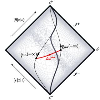
Figure 3: Scattering of a massive particle in a “sandwich” plane wave geometry. The interacting trajectory is matched with free-theory worldlines in the in- and out-regions. The “classical S-matrix” is then defined as a map acting on the representative free-particle states.

“Exact amplitude”

Now we are ready to compute (130) for various classical observables. Using (132), the infinite time limit of (122b) is found as

$$\begin{split}L^{\dot{\alpha}}{}_{\dot{\beta}}({-}\infty,{+}\infty)\,=\,\delta^{\dot{\alpha}}{}_{\dot{\beta}}+i\hskip 0.50003pt{\mathcal{M}}^{+}\hskip 1.00006pt\delta\kern-1.99997pt\makebox[0.0pt][l]{$\bar{}$}\kern 1.99997pt(2\hskip 1.00006pt{\mathsf{3}}{\hskip 1.00006pt\cdot\hskip 1.00006pt}{\mathsf{1}})\hskip 1.00006pt({\bar{\mathsf{3}}}^{\dot{\alpha}}{\bar{\mathsf{3}}}_{\dot{\beta}}/mx)\,,\quad{\mathcal{M}}^{+}:=\nu mx\hskip 1.00006pt\hskip 0.50003pt{\mathrm{e}}^{{\mathsf{3}}\cdot(a+ib)}\,,\end{split}$$ (133)

from which it follows that the minimal momentum impulse and amplitude found in Section 3.3 are reproduced as exact quantities. Besides, as expected from $\dot{W}^{a}=0$, we find that $y^{{\dot{\alpha}}\alpha}$ experiences the same chiral null rotation as $p_{\alpha{\dot{\alpha}}}$:

$$\mathit{\Delta}p_{\alpha{\dot{\alpha}}} =i\hskip 0.50003pt{\mathcal{M}}^{+}\hskip 1.00006pt\delta\kern-1.99997pt\makebox[0.0pt][l]{$\bar{}$}\kern 1.99997pt(2\hskip 1.00006pt{\mathsf{3}}{\hskip 1.00006pt\cdot\hskip 1.00006pt}{\mathsf{1}})\,{\mathsf{1}}_{\smash{\alpha{\dot{\beta}}}\vphantom{{\dot{\alpha}}}}\hskip 0.50003pt({\bar{\mathsf{3}}}^{\dot{\beta}}{\bar{\mathsf{3}}}_{\dot{\alpha}}/mx)=i\hskip 0.50003pt{\mathcal{M}}^{+}\hskip 1.00006pt\delta\kern-1.99997pt\makebox[0.0pt][l]{$\bar{}$}\kern 1.99997pt(2\hskip 1.00006pt{\mathsf{3}}{\hskip 1.00006pt\cdot\hskip 1.00006pt}{\mathsf{1}})\,{\mathsf{3}}_{\alpha{\dot{\alpha}}}\,,$$ (134a)

$$\mathit{\Delta}y^{{\dot{\alpha}}\alpha} =i\hskip 0.50003pt{\mathcal{M}}^{+}\hskip 1.00006pt\delta\kern-1.99997pt\makebox[0.0pt][l]{$\bar{}$}\kern 1.99997pt(2\hskip 1.00006pt{\mathsf{3}}{\hskip 1.00006pt\cdot\hskip 1.00006pt}{\mathsf{1}})\,({\bar{\mathsf{3}}}^{\dot{\alpha}}{\bar{\mathsf{3}}}_{\dot{\beta}}/mx)\hskip 1.00006pta^{{\dot{\beta}}\alpha}\,.$$ (134b)

For the spinorial frame impulse, however, there are additional $\mathrm{SU}(2)$ factors due to $\delta\tau_{*}:=\tau_{*}({-}\infty,{+}\infty)-\tau_{*}({-}\infty,{-}\infty)$:

$$\begin{split}\smash{\underset{\scalebox{0.8}[0.8]{\leavevmode\hbox{\raise 1.99997pt\hbox{\set@color\resizebox{}{}{{\leavevmode\hbox{\set@color{$*$}}}}}}}}{\lambda}{}_{\alpha}{}^{I}({+}\infty)}&={\mathsf{1}}_{\alpha}{}^{J}\exp\big{(}\hskip 0.50003pt{\delta\tau_{*}\hskip 1.00006pt\Omega^{a}(\sigma_{a})/2i}\hskip 0.50003pt\big{)}{}_{J}{}^{I}\,,\\ \smash{\underset{\scalebox{0.8}[0.8]{\leavevmode\hbox{\raise 1.99997pt\hbox{\set@color\resizebox{}{}{{\leavevmode\hbox{\set@color{$*$}}}}}}}}{{\bar{\lambda}}}{}_{I{\dot{\alpha}}}({+}\infty)}&=\exp\big{(}\hskip 0.50003pt{-\delta\tau_{*}\hskip 1.00006pt\Omega^{a}(\sigma_{a})/2i}\hskip 0.50003pt\big{)}{}_{I}{}^{J}\hskip 1.00006pt{\bar{\mathsf{1}}}_{\smash{J{\dot{\beta}}}\vphantom{I{\dot{\alpha}}}}\hskip 1.00006ptL^{\dot{\beta}}{}_{\dot{\alpha}}({-}\infty,{+}\infty)\,.\end{split}$$ (135)

Putting $\Omega^{a}=0$ recovers the result of Section 3.3. One finds from (128) that

$$\delta\tau_{*} \hskip 1.00006pt=\hskip 1.00006pt{\mathcal{M}}^{+}\hskip 0.50003pt\delta\kern-1.99997pt\makebox[0.0pt][l]{$\bar{}$}\kern 1.99997pt(2\hskip 1.00006pt{\mathsf{3}}{\hskip 1.00006pt\cdot\hskip 1.00006pt}{\mathsf{1}})\,({\mathsf{3}}{\hskip 1.00006pt\cdot\hskip 1.00006pt}(a{\hskip 1.00006pt+\hskip 1.00006pt}ib)/m)\,.$$ (136)

Angular momentum impulses

The orbital and spin angular momenta of the particle are given as $L_{mn}:=2x_{[m}p_{n]}$ and $S_{mn}:=\varepsilon_{mnrs}{\hskip 0.50003pt}y^{r}{}p^{s}$. In the spinor notation, the total angular momentum $J_{mn}:=L_{mn}+S_{mn}$ is given by

$$J^{\dot{\alpha}}{}_{\dot{\beta}}=-z^{{\dot{\alpha}}\alpha}p_{\alpha{\dot{\beta}}}+{\textstyle\frac{1}{2}}\hskip 1.00006pt\delta^{\dot{\alpha}}{}_{\dot{\beta}}\hskip 0.50003pt(z^{{\dot{{\gamma}}}{\gamma}}p_{{\gamma}{\dot{{\gamma}}}})\,,\quad\bar{J}_{\alpha}{}^{\beta}=-p_{\alpha{\dot{\alpha}}}{\bar{z}}^{{\dot{\alpha}}\beta}+{\textstyle\frac{1}{2}}\hskip 1.00006pt\delta_{\alpha}{}^{\beta}\hskip 0.50003pt(p_{{\gamma}{\dot{{\gamma}}}}{\bar{z}}^{{\dot{{\gamma}}}{\gamma}})\,.$$ (137)

Since $L_{mn}$, $S_{mn}$, and $J_{mn}$ are all conserved quantities in the free theory, we can use the interaction-picture expressions for computing their impulse.

First, we find from (134) that

$${\begin{array}[]{rl}\mathit{\Delta}\bar{S}_{\alpha}{}^{\beta}=0\,,\quad\mathit{\Delta}S^{\dot{\alpha}}{}_{\dot{\beta}}&{}={\mathcal{M}}^{+}\,\delta\kern-1.99997pt\makebox[0.0pt][l]{$\bar{}$}\kern 1.99997pt(2\hskip 1.00006pt{\mathsf{3}}{\hskip 1.00006pt\cdot\hskip 1.00006pt}{\mathsf{1}})\,\big{(}|{\bar{\mathsf{3}}}{\kern-0.39993pt\leavevmode\hbox{$\vbox{\hbox{\resizebox{}{}{\scalebox{0.99}[0.99]{{\leavevmode\hbox{\set@color{${\hbox to0.0pt{\reflectbox{\rotatebox[origin={c}]{180.0}{$\rfloor$}}\hss}\rfloor}$}}}}}}}$}\kern-0.37003pt}{\kern-0.37003pt\leavevmode\hbox{$\vbox{\hbox{\resizebox{}{}{\scalebox{0.99}[0.99]{{\leavevmode\hbox{\set@color{${\lfloor\hbox to0.0pt{\hss\reflectbox{\rotatebox[origin={c}]{180.0}{$\lfloor$}}}}$}}}}}}}$}\kern-0.39993pt}{\bar{\mathsf{3}}}|a|{\mathsf{1}}|-|a|{\mathsf{1}}|{\bar{\mathsf{3}}}{\kern-0.39993pt\leavevmode\hbox{$\vbox{\hbox{\resizebox{}{}{\scalebox{0.99}[0.99]{{\leavevmode\hbox{\set@color{${\hbox to0.0pt{\reflectbox{\rotatebox[origin={c}]{180.0}{$\rfloor$}}\hss}\rfloor}$}}}}}}}$}\kern-0.37003pt}{\kern-0.37003pt\leavevmode\hbox{$\vbox{\hbox{\resizebox{}{}{\scalebox{0.99}[0.99]{{\leavevmode\hbox{\set@color{${\lfloor\hbox to0.0pt{\hss\reflectbox{\rotatebox[origin={c}]{180.0}{$\lfloor$}}}}$}}}}}}}$}\kern-0.39993pt}{\bar{\mathsf{3}}}|\big{)}{}^{\dot{\alpha}}{}_{\dot{\beta}}/mx\,,\\ &{}={\mathcal{M}}^{+}\,\delta\kern-1.99997pt\makebox[0.0pt][l]{$\bar{}$}\kern 1.99997pt(2\hskip 1.00006pt{\mathsf{3}}{\hskip 1.00006pt\cdot\hskip 1.00006pt}{\mathsf{1}})\,({\mathsf{3}}^{{\dot{\alpha}}\alpha}a_{\smash{\alpha{\dot{\beta}}}\vphantom{\beta}}-a^{{\dot{\alpha}}\alpha}{\mathsf{3}}_{\smash{\alpha{\dot{\beta}}}\vphantom{\beta}})\,,\\ &{}=i\hskip 0.50003pt{\mathcal{M}}^{+}\,\delta\kern-1.99997pt\makebox[0.0pt][l]{$\bar{}$}\kern 1.99997pt(2\hskip 1.00006pt{\mathsf{3}}{\hskip 1.00006pt\cdot\hskip 1.00006pt}{\mathsf{1}})\,(-\varepsilon_{mnrs}\hskip 0.50003pta^{r}{\mathsf{3}}^{s})\hskip 0.50003pt({\bar{\sigma}}^{mn})^{\dot{\alpha}}{}_{\dot{\beta}}\,,\end{array}}$$ (141)

which is consistent with the chiral Lorentz transformation interpretation.

Next, we compute $\mathit{\Delta}J^{\dot{\alpha}}{}_{\dot{\beta}}$. The $(\tau_{*}{-\hskip 1.00006pt}\tau_{0})\hskip 1.00006ptL^{\dot{\alpha}}{}_{\dot{\beta}}(\tau,\tau_{0})\hskip 0.50003ptu^{{\dot{\beta}}\alpha}\propto(p^{-1}(\tau))^{{\dot{\alpha}}\alpha}$ term in (126d) does not boil down to a particularly neat expression in the infinite time limit, but it drops out when one computes $p_{\alpha{\dot{\alpha}}}(\tau)\hskip 1.00006pt\smash{\underset{\scalebox{0.8}[0.8]{\leavevmode\hbox{\raise 1.99997pt\hbox{\set@color\resizebox{}{}{{\leavevmode\hbox{\set@color{$*$}}}}}}}}{z}{}^{{\dot{\alpha}}\beta}(\tau)}$ or $\smash{\underset{\scalebox{0.8}[0.8]{\leavevmode\hbox{\raise 1.99997pt\hbox{\set@color\resizebox{}{}{{\leavevmode\hbox{\set@color{$*$}}}}}}}}{z}{}^{{\dot{\alpha}}\alpha}(\tau)}\hskip 1.00006ptp_{\smash{\alpha{\dot{\beta}}}\vphantom{\alpha{\dot{\alpha}}}}(\tau)$ and symmetrizes the two spinor indices. As a result, we find

$$\begin{split}\mathit{\Delta}J^{\smash{{\dot{\alpha}}{\dot{\beta}}}\vphantom{({\dot{\alpha}}}}\hskip 1.00006pt&=\hskip 1.00006pti\hskip 0.50003pt{\mathcal{M}}^{+}\hskip 1.00006pt\delta\kern-1.99997pt\makebox[0.0pt][l]{$\bar{}$}\kern 1.99997pt(2\hskip 1.00006pt{\mathsf{3}}{\hskip 1.00006pt\cdot\hskip 1.00006pt}{\mathsf{1}})\hskip 1.00006pt\big{(}{-z_{\smash{*}}^{({\dot{\alpha}}\alpha}\hskip 0.50003pt{\mathsf{3}}_{\alpha}\vphantom{z}^{\smash{{\dot{\beta}})}\vphantom{({\dot{\alpha}}}}}\big{)}\,,\\ \mathit{\Delta}L^{\smash{{\dot{\alpha}}{\dot{\beta}}}\vphantom{({\dot{\alpha}}}}\hskip 1.00006pt&=\hskip 1.00006pti\hskip 0.50003pt{\mathcal{M}}^{+}\hskip 1.00006pt\delta\kern-1.99997pt\makebox[0.0pt][l]{$\bar{}$}\kern 1.99997pt(2\hskip 1.00006pt{\mathsf{3}}{\hskip 1.00006pt\cdot\hskip 1.00006pt}{\mathsf{1}})\hskip 1.00006pt\big{(}{-(z_{\smash{*}}\hskip 0.50003pt{+}\hskip 1.00006pt2ia)^{({\dot{\alpha}}\alpha}\hskip 0.50003pt{\mathsf{3}}_{\alpha}\vphantom{z}^{\smash{{\dot{\beta}})}\vphantom{({\dot{\alpha}}}}}\big{)}\,,\\ \mathit{\Delta}\bar{J}^{\smash{\alpha\beta}\vphantom{({\dot{\alpha}}}}\hskip 1.00006pt=\hskip 1.00006pt\mathit{\Delta}\bar{L}^{\smash{\alpha\beta}\vphantom{({\dot{\alpha}}}}\hskip 1.00006pt&=\hskip 1.00006pti\hskip 0.50003pt{\mathcal{M}}^{+}\hskip 1.00006pt\delta\kern-1.99997pt\makebox[0.0pt][l]{$\bar{}$}\kern 1.99997pt(2\hskip 1.00006pt{\mathsf{3}}{\hskip 1.00006pt\cdot\hskip 1.00006pt}{\mathsf{1}})\,\big{(}{-{\mathsf{3}}^{(\alpha}{}_{\dot{\alpha}}\hskip 0.50003ptz_{\smash{*}}^{{\dot{\alpha}}\beta)}}\big{)}\,,\end{split}$$ (142)

noting that

$$G^{\dot{\alpha}}{}_{\dot{\beta}}({+}\infty,{-}\infty)=(2/x)\hskip 1.00006pt{\mathcal{M}}^{+}\hskip 0.50003pt\delta\kern-1.99997pt\makebox[0.0pt][l]{$\bar{}$}\kern 1.99997pt^{\prime}(2\hskip 1.00006pt{\mathsf{3}}{\hskip 1.00006pt\cdot\hskip 1.00006pt}{\mathsf{1}})\,{\bar{\mathsf{3}}}^{\dot{\alpha}}{\bar{\mathsf{3}}}_{\dot{\beta}}\hskip 1.00006pt=(2/m)\hskip 1.00006pt{\mathcal{M}}^{+}\hskip 0.50003pt\delta\kern-1.99997pt\makebox[0.0pt][l]{$\bar{}$}\kern 1.99997pt^{\prime}(2\hskip 1.00006pt{\mathsf{3}}{\hskip 1.00006pt\cdot\hskip 1.00006pt}{\mathsf{1}})\,{\mathsf{1}}^{{\dot{\alpha}}\alpha}{\mathsf{3}}_{\smash{\alpha{\dot{\beta}}}\vphantom{{\dot{\alpha}}}}\,.$$ (143)

We have defined

$$z_{\smash{*}}^{{\dot{\alpha}}\alpha}\hskip 1.00006pt:=\hskip 1.00006pt(b-ia)^{{\dot{\alpha}}\alpha}+u^{{\dot{\alpha}}\alpha}\hskip 1.00006ptT\,,\quad T:=-im/({\mathsf{3}}{\hskip 1.00006pt\cdot\hskip 1.00006pt}{\mathsf{1}})-u\cdot z({-}\infty)\,,$$ (144)

which has a natural interpretation as the intersection point of the initial and final asymptotic holomorphic worldlines. The existence of such a point is not a trivial fact and is a consequence of the special geometry of this scattering problem.

To sum up, (142) boils down to

$$\begin{split}\mathit{\Delta}S^{mn}&=i\hskip 0.50003pt{\mathcal{M}}^{+}\hskip 1.00006pt\delta\kern-1.99997pt\makebox[0.0pt][l]{$\bar{}$}\kern 1.99997pt(2\hskip 1.00006pt{\mathsf{3}}{\hskip 1.00006pt\cdot\hskip 1.00006pt}{\mathsf{1}})\hskip 1.00006pt\big{(}\hskip 1.00006pt{-2i\hskip 1.00006pta^{[m}{\mathsf{3}}^{n]}-\varepsilon^{mnrs}a_{r}{\mathsf{3}}_{s}}\big{)}\,,\\ \mathit{\Delta}L^{mn}&=i\hskip 0.50003pt{\mathcal{M}}^{+}\hskip 1.00006pt\delta\kern-1.99997pt\makebox[0.0pt][l]{$\bar{}$}\kern 1.99997pt(2\hskip 1.00006pt{\mathsf{3}}{\hskip 1.00006pt\cdot\hskip 1.00006pt}{\mathsf{1}})\hskip 1.00006pt\big{(}\hskip 1.00006pt{2\hskip 1.00006pt{\mathsf{1}}^{[m}{\mathsf{3}}^{n]}(T/m)+2b^{[m}{\mathsf{3}}^{n]}+\varepsilon^{mnrs}a_{r}{\mathsf{3}}_{s}}\big{)}\,,\\ \mathit{\Delta}J^{mn}&=i\hskip 0.50003pt{\mathcal{M}}^{+}\hskip 1.00006pt\delta\kern-1.99997pt\makebox[0.0pt][l]{$\bar{}$}\kern 1.99997pt(2\hskip 1.00006pt{\mathsf{3}}{\hskip 1.00006pt\cdot\hskip 1.00006pt}{\mathsf{1}})\hskip 1.00006pt\big{(}\hskip 1.00006pt{2\hskip 1.00006pt{\mathsf{1}}^{[m}{\mathsf{3}}^{n]}(T/m)+2b^{[m}{\mathsf{3}}^{n]}-2i\hskip 1.00006pta^{[m}{\mathsf{3}}^{n]}}\big{)}\,.\end{split}$$ (145)

Note that only $\mathit{\Delta}J^{mn}=i\hskip 0.50003pt{\mathcal{M}}^{+}\hskip 1.00006pt\delta\kern-1.99997pt\makebox[0.0pt][l]{$\bar{}$}\kern 1.99997pt(2\hskip 1.00006pt{\mathsf{3}}{\hskip 1.00006pt\cdot\hskip 1.00006pt}{\mathsf{1}})\,z_{\smash{*}}^{[m}{\mathsf{3}}^{n]}$ is “polar.” The other two have “axial” components, i.e., terms involving the epsilon tensor. Especially, the orbital angular momentum impulse $\mathit{\Delta}L^{mn}$ is not polar. One may interpret this fact as a failure of a local particle interpretation in real spacetime (and the necessity of complex spacetime).

Exact $\sqrt{\text{Kerr\hskip 0.50003pt}}$ impulses

Finally, let us re-solve the equation of motion with (114). We start off with $\sqrt{\text{Kerr\hskip 0.50003pt}}$. For clarity’s sake, we spell out the entire symplectic form:

$${\begin{array}[]{rl}\omega_{{{\text{$\sqrt{\text{Kerr\hskip 0.35002pt}}$}}}}^{\text{SDPW}}\,={}&{}i\hskip 1.00006ptd{\bar{Z}}_{I}{}^{\mathrm{A}}{\hskip 1.00006pt{\wedge}\,}dZ_{\mathrm{A}}{}^{I}+i\hskip 0.50003ptd{\smash{\bar{\psi}}\kern 0.20004pt\vphantom{\psi}}_{i}{\hskip 1.00006pt{\wedge}\,}d\psi^{i}\\ {}\hfil&{}{}+\sqrt{2}g\,dq_{a}c^{a}{\hskip 1.00006pt{\wedge}\,}{\kern-0.37003pt\leavevmode\hbox{$\vbox{\hbox{\resizebox{}{}{\scalebox{0.99}[0.99]{{\leavevmode\hbox{\set@color{${\lfloor\hbox to0.0pt{\hss\reflectbox{\rotatebox[origin={c}]{180.0}{$\lfloor$}}}}$}}}}}}}$}\kern-0.39993pt}{\bar{o}}|dz|\iota\rangle\hskip 1.00006pt{\mathrm{e}}^{-i\hskip 0.35002pt{\bar{o}zo}}+{\textstyle\frac{ig}{\sqrt{2}}}\hskip 1.00006ptq_{a}c^{a}\hskip 1.00006pt{\bar{o}}_{\dot{\alpha}}\hskip 0.50003pt{\bar{o}}_{\dot{\beta}}(dz{\hskip 1.00006pt{\wedge}\,}dz)^{{\dot{\alpha}}{\dot{\beta}}}\hskip 1.00006pt{\mathrm{e}}^{-i\hskip 0.35002pt{\bar{o}zo}}\,.\end{array}}$$ (148)

The resulting equation of motion boils down to

$$\begin{split}\dot{\lambda}_{\alpha}{}^{I}={\textstyle\frac{1}{2i}}(\lambda\hskip 0.50003pt\sigma_{a})_{\alpha}{}^{I}&\,,\quad\dot{{\bar{\lambda}}}_{I{\dot{\alpha}}}=(i\nu{/}2m)\hskip 1.00006pt{\bar{\lambda}}_{\smash{I{\dot{\beta}}}\vphantom{I}}\hskip 1.00006pt{\bar{o}}^{\dot{\beta}}{\bar{o}}_{\dot{\alpha}}\hskip 1.00006pt{\mathrm{e}}^{-i\hskip 0.35002pt{\bar{o}zo}}-{\textstyle\frac{1}{2i}}(\sigma_{a}{\bar{\lambda}})_{I{\dot{\alpha}}}\,,\\ \dot{z}^{{\dot{\alpha}}\alpha}={\textstyle\frac{1}{-2}}m(p^{-1})^{{\dot{\alpha}}\alpha}&\,,\quad\dot{y}^{{\dot{\alpha}}\alpha}=-(i\nu{/}2m)\hskip 1.00006pt{\bar{o}}^{\dot{\alpha}}{\bar{o}}_{\dot{\beta}}\hskip 1.00006pty^{{\dot{\beta}}\alpha}\hskip 1.00006pt{\mathrm{e}}^{-i\hskip 0.35002pt{\bar{o}zo}}\,,\end{split}$$ (149a)

$$\dot{\psi}^{i}=-({\textstyle\frac{g}{\sqrt{2}}}\tilde{x}\hskip 0.50003ptc^{a})\hskip 1.00006pt(t_{a})^{i}{}_{j}\hskip 0.24994pt\psi^{j}\hskip 0.50003pt\hskip 1.00006pt{\mathrm{e}}^{-i\hskip 0.35002pt{\bar{o}zo}} \,,\quad\dot{\bar{\psi}}_{i}=({\textstyle\frac{g}{\sqrt{2}}}\tilde{x}\hskip 0.50003ptc^{a})\hskip 1.00006pt{\smash{\bar{\psi}}\kern 0.20004pt\vphantom{\psi}}_{j}(t_{a})^{j}{}_{i}\hskip 0.50003pt\hskip 1.00006pt{\mathrm{e}}^{-i\hskip 0.35002pt{\bar{o}zo}}\,.$$ (149b)

The last line implies $\dot{q}_{a}=(q_{b}f^{b}{}_{ca}\hskip 0.24994ptc^{c})\hskip 1.00006pt{\textstyle\frac{g}{\sqrt{2}}}\tilde{x}\,{\mathrm{e}}^{-i\hskip 0.35002pt{\bar{o}zo}}$. We have defined the “off-shell $x$-factor”

$$\tilde{x}:=-\langle\iota|p|{\bar{o}}{\kern-0.39993pt\leavevmode\hbox{$\vbox{\hbox{\resizebox{}{}{\scalebox{0.99}[0.99]{{\leavevmode\hbox{\set@color{${\hbox to0.0pt{\reflectbox{\rotatebox[origin={c}]{180.0}{$\rfloor$}}\hss}\rfloor}$}}}}}}}$}\kern-0.37003pt}/|\Delta|\,,$$ (150)

which is a constant of motion. Note that both “holomorphic” and “anti-holomorphic” color degrees of freedom, $\psi^{i}$ and ${\smash{\bar{\psi}}\kern 0.20004pt\vphantom{\psi}}_{i}$, are localized at the holomorphic position $z^{{\dot{\alpha}}\alpha}$, being parallel-transported by the holomorphic gauge connection. Indeed, both $\psi^{i}$ and ${\smash{\bar{\psi}}\kern 0.20004pt\vphantom{\psi}}_{i}$ should couple to the holomorphic connection for $q_{a}F^{a}(z)=(i\hskip 0.50003pt{\smash{\bar{\psi}}\kern 0.20004pt\vphantom{\psi}}\hskip 0.50003ptt_{a}\psi)F^{a}(z)$ to be gauge invariant.

We can understand (149) as a combination of an infinitesimal self-dual null rotation, color rotation, and internal $\mathrm{SU}(2)$ rotation with fixed points ${\bar{o}}^{\dot{\alpha}}$, $c^{a}$, and $\Omega^{a}$, respectively. Hence, $\nu=\sqrt{2}g\hskip 1.00006ptq_{a}c^{a}$ is conserved.

Now, since (149a) is totally unaffected by the $dq{\hskip 1.00006pt{\wedge}\,}dz$ correction, it follows that the solution (121) and the impulses (134)-(145) are all valid. The only additional piece of information is the color time evolution and impulse that follow from (149b):

$$\psi^{i}(\tau) =U^{i}{}_{j}(\tau,\tau_{0})\hskip 1.00006pt\psi^{j}(\tau_{0})\,,\quad{\smash{\bar{\psi}}\kern 0.20004pt\vphantom{\psi}}_{i}(\tau)={\smash{\bar{\psi}}\kern 0.20004pt\vphantom{\psi}}_{j}(\tau_{0})\hskip 1.00006ptU^{j}{}_{i}(\tau_{0},\tau)\,,$$ (151a)

$$U^{i}{}_{j}(\tau_{2},\tau_{1}) =\exp\left(\hskip 0.50003pt{\frac{g\tilde{x}}{\sqrt{2}}\hskip 1.00006ptc^{a}(t_{a})\,{\mathrm{e}}^{i{\mathsf{3}}\cdot(z(\tau_{0})-u\tau_{0})}\int_{\tau_{1}}^{\tau_{2}}d\tau^{\prime}\,\hskip 1.00006pt{\mathrm{e}}^{i({\mathsf{3}}\cdot u)\tau^{\prime}}}\hskip 0.24994pt\right){\vphantom{\Big{|}}}^{i}{\vphantom{\Big{|}}}_{j}\,,$$ (151b)

$$U^{i}{}_{j}({+}\infty,{-}\infty) =\exp\left(\hskip 1.00006pt{i\hskip 0.50003pt{\mathcal{M}}^{+1}({\mathsf{1}},a;{\mathsf{3}})\hskip 1.00006pt{\mathrm{e}}^{i{\mathsf{3}}\cdot b}\hskip 1.00006pt\delta\kern-1.99997pt\makebox[0.0pt][l]{$\bar{}$}\kern 1.99997pt(2\hskip 1.00006pt{\mathsf{3}}{\hskip 1.00006pt\cdot\hskip 1.00006pt}{\mathsf{1}})\hskip 1.00006ptc^{a}\hskip 1.00006pti(t_{a})}\hskip 0.24994pt\right){\vphantom{\big{|}}}^{i}{\vphantom{\big{|}}}_{j}\,.$$ (151c)

Note that $\smash{\underset{\scalebox{0.8}[0.8]{\leavevmode\hbox{\raise 1.99997pt\hbox{\set@color\resizebox{}{}{{\leavevmode\hbox{\set@color{$*$}}}}}}}}{\psi}{\vphantom{\psi}}^{i}(\tau)}=\psi^{i}(\tau)$ and $\smash{\underset{\scalebox{0.8}[0.8]{\leavevmode\hbox{\raise 1.99997pt\hbox{\set@color\resizebox{}{}{{\leavevmode\hbox{\set@color{$*$}}}}}}}}{{\smash{\bar{\psi}}\kern 0.20004pt\vphantom{\psi}}}{\vphantom{{\smash{\bar{\psi}}\kern 0.20004pt\vphantom{\psi}}}}_{i}(\tau)}={\smash{\bar{\psi}}\kern 0.20004pt\vphantom{\psi}}_{i}(\tau)$, since $\dot{\psi}^{i}=0$ and $\dot{\bar{\psi}}_{i}=0$ in the free theory. The color rotation (151b) may be thought of as the “square root” of the chiral Lorentz transformation (122b) or the additional null translation (156) which we derive shortly. The time evolution and the impulse of the color charge $q_{a}$ easily follow from translating (151b)-(151c) to the adjoint representation. One may expand the exponential and find

$$\begin{split}\mathit{\Delta}\psi^{i}\hskip 1.00006pt&=\hskip 1.00006pti\hskip 0.50003pt{\mathcal{M}}^{+1}({\mathsf{1}},a;{\mathsf{3}})\hskip 1.00006pt{\mathrm{e}}^{i{\mathsf{3}}\cdot b}\hskip 1.00006pt\delta\kern-1.99997pt\makebox[0.0pt][l]{$\bar{}$}\kern 1.99997pt(2\hskip 1.00006pt{\mathsf{3}}{\hskip 1.00006pt\cdot\hskip 1.00006pt}{\mathsf{1}})\,(\hskip 0.24994pt(t_{c})^{i}{}_{j}\hskip 0.50003pt\psi^{j}\hskip 0.24994pt)\hskip 1.00006ptic^{c}+\mathcal{O}(g^{2})\,,\\ \mathit{\Delta}{\smash{\bar{\psi}}\kern 0.20004pt\vphantom{\psi}}_{i}\hskip 1.00006pt&=\hskip 1.00006pti\hskip 0.50003pt{\mathcal{M}}^{+1}({\mathsf{1}},a;{\mathsf{3}})\hskip 1.00006pt{\mathrm{e}}^{i{\mathsf{3}}\cdot b}\hskip 1.00006pt\delta\kern-1.99997pt\makebox[0.0pt][l]{$\bar{}$}\kern 1.99997pt(2\hskip 1.00006pt{\mathsf{3}}{\hskip 1.00006pt\cdot\hskip 1.00006pt}{\mathsf{1}})\,(\hskip 0.24994pt-{\smash{\bar{\psi}}\kern 0.20004pt\vphantom{\psi}}_{j}(t_{c})^{j}{}_{i}\hskip 0.24994pt)\hskip 1.00006ptic^{c}+\mathcal{O}(g^{2})\,,\\ \mathit{\Delta}q_{a}\hskip 1.00006pt&=\hskip 1.00006pti\hskip 0.50003pt{\mathcal{M}}^{+1}({\mathsf{1}},a;{\mathsf{3}})\hskip 1.00006pt{\mathrm{e}}^{i{\mathsf{3}}\cdot b}\hskip 1.00006pt\delta\kern-1.99997pt\makebox[0.0pt][l]{$\bar{}$}\kern 1.99997pt(2\hskip 1.00006pt{\mathsf{3}}{\hskip 1.00006pt\cdot\hskip 1.00006pt}{\mathsf{1}})\,(\hskip 0.24994pt-q_{b}\hskip 0.50003ptf^{b}{}_{ca}\hskip 0.24994pt)\hskip 1.00006ptic^{c}+\mathcal{O}(g^{2})\,.\end{split}$$ (152)

Exact Kerr impulses

For Kerr in the self-dual gravitational plane wave, the symplectic form is given by

$$\begin{split}{\begin{array}[]{rl}\omega_{\text{Kerr}}^{\text{SDPW}}\,={}&{}i\hskip 1.00006ptd{\bar{Z}}_{I}{}^{\mathrm{A}}{\hskip 1.00006pt{\wedge}\,}dZ_{\mathrm{A}}{}^{I}\\ {}\hfil&{}\displaystyle-\frac{1}{{M_{\text{Pl}}}}\hskip 1.00006pt\langle\iota|dp|{\bar{o}}{\kern-0.39993pt\leavevmode\hbox{$\vbox{\hbox{\resizebox{}{}{\scalebox{0.99}[0.99]{{\leavevmode\hbox{\set@color{${\hbox to0.0pt{\reflectbox{\rotatebox[origin={c}]{180.0}{$\rfloor$}}\hss}\rfloor}$}}}}}}}$}\kern-0.37003pt}{\hskip 0.50003pt\wedge\hskip 0.50003pt}{\kern-0.37003pt\leavevmode\hbox{$\vbox{\hbox{\resizebox{}{}{\scalebox{0.99}[0.99]{{\leavevmode\hbox{\set@color{${\lfloor\hbox to0.0pt{\hss\reflectbox{\rotatebox[origin={c}]{180.0}{$\lfloor$}}}}$}}}}}}}$}\kern-0.39993pt}{\bar{o}}|dz|\iota\rangle\hskip 1.00006pt{\mathrm{e}}^{-i\hskip 0.35002pt{\bar{o}zo}}+\frac{im\tilde{x}}{2{M_{\text{Pl}}}}\hskip 1.00006pt{\bar{o}}_{\dot{\alpha}}\hskip 0.50003pt{\bar{o}}_{\dot{\beta}}\hskip 0.24994pt(dz{\hskip 1.00006pt{\wedge}\,}dz)^{{\dot{\alpha}}{\dot{\beta}}}\hskip 1.00006pt{\mathrm{e}}^{-i\hskip 0.35002pt{\bar{o}zo}}\,.\end{array}}\end{split}$$ (153)

The equation of motion reads

$$\begin{split}\dot{{\bar{\lambda}}}_{I{\dot{\alpha}}}=(i\nu{/}2m)\hskip 1.00006pt{\bar{\lambda}}_{\smash{I{\dot{\beta}}}\vphantom{I}}\hskip 1.00006pt{\bar{o}}^{\dot{\beta}}{\bar{o}}_{\dot{\alpha}}\hskip 1.00006pt{\mathrm{e}}^{-i\hskip 0.35002pt{\bar{o}zo}}-{\textstyle\frac{1}{2i}}(\sigma_{a}{\bar{\lambda}})_{I{\dot{\alpha}}}&\,,\quad\dot{\lambda}_{\alpha}{}^{I}={\textstyle\frac{1}{2i}}(\lambda\hskip 0.50003pt\sigma_{a})_{\alpha}{}^{I}\,,\\ \dot{z}^{{\dot{\alpha}}\alpha}={\textstyle\frac{1}{-2}}\big{(}\hskip 0.50003pt{m(p^{-1})^{{\dot{\alpha}}\alpha}{\hskip 0.50003pt-\hskip 1.00006pt}(\nu{/}m)\hskip 1.00006pt{{\bar{o}}^{\dot{\alpha}}\iota^{\alpha}}\hskip 1.00006pt{\mathrm{e}}^{-i\hskip 0.35002pt{\bar{o}zo}}}\hskip 1.00006pt\big{)}&\,,\quad\dot{y}^{{\dot{\alpha}}\alpha}=-(i\nu{/}2m)\hskip 1.00006pt{\bar{o}}^{\dot{\alpha}}{\bar{o}}_{\dot{\beta}}\hskip 1.00006pty^{{\dot{\beta}}\alpha}\hskip 1.00006pt{\mathrm{e}}^{-i\hskip 0.35002pt{\bar{o}zo}}\,.\end{split}$$ (154)

The additional “zitterbewegung” of $z^{{\dot{\alpha}}\alpha}$ lies within the ${\dot{\alpha}}$-plane of $|{\bar{o}}{\kern-0.39993pt\leavevmode\hbox{$\vbox{\hbox{\resizebox{}{}{\scalebox{0.99}[0.99]{{\leavevmode\hbox{\set@color{${\hbox to0.0pt{\reflectbox{\rotatebox[origin={c}]{180.0}{$\rfloor$}}\hss}\rfloor}$}}}}}}}$}\kern-0.37003pt}$. As a result, $\nu{\hskip 1.00006pt=\hskip 1.00006pt}$ $(m{/}{M_{\text{Pl}}})\hskip 0.50003pt\tilde{x}$ is conserved, and (120) is valid. This means that the solution (121) holds except for $z^{{\dot{\alpha}}\alpha}(\tau)$. The revised solution for $z^{{\dot{\alpha}}\alpha}(\tau)$ is given as

$$z^{{\dot{\alpha}}\alpha}(\tau)\hskip 1.00006pt=\hskip 1.00006ptz^{{\dot{\alpha}}\alpha}(\tau_{0})+F^{\dot{\alpha}}{}_{\dot{\beta}}(\tau,\tau_{0})\hskip 1.00006ptu^{{\dot{\beta}}\alpha}+X^{{\dot{\alpha}}\alpha}(\tau,\tau_{0})\,,$$ (155)

where the new contribution $X^{{\dot{\alpha}}\alpha}(\tau,\tau_{0})$ is given by

$$X^{{\dot{\alpha}}\alpha}(\tau,\tau_{0})\hskip 1.00006pt:={} \hskip 1.00006pt\frac{\tilde{x}\hskip 1.00006pt{\bar{o}}^{\dot{\alpha}}\iota^{\alpha}}{2{M_{\text{Pl}}}}\hskip 1.00006pt{\mathrm{e}}^{i{\mathsf{3}}\cdot(z(\tau_{0})-u\tau_{0})}\int_{\tau_{0}}^{\tau}d\tau^{\prime}\,\hskip 1.00006pt{\mathrm{e}}^{i({\mathsf{3}}\cdot u)\tau^{\prime}}\,,$$ (156)

$${{\implies}\quad}X^{{\dot{\alpha}}\alpha}({+}\infty,{-}\infty)\hskip 1.00006pt={} \hskip 1.00006pt{\mathcal{M}}^{+2}({\mathsf{1}},a;{\mathsf{3}})\hskip 1.00006pt{\mathrm{e}}^{i{\mathsf{3}}\cdot b}\hskip 1.00006pt\delta\kern-1.99997pt\makebox[0.0pt][l]{$\bar{}$}\kern 1.99997pt(2\hskip 1.00006pt{\mathsf{3}}{\hskip 1.00006pt\cdot\hskip 1.00006pt}{\mathsf{1}})\,({\bar{o}}^{\dot{\alpha}}\iota^{\alpha}/mx)\,.$$ (157)

Accordingly, we have

$$\smash{\underset{\scalebox{0.8}[0.8]{\leavevmode\hbox{\raise 1.99997pt\hbox{\set@color\resizebox{}{}{{\leavevmode\hbox{\set@color{$*$}}}}}}}}{z}{}^{{\dot{\alpha}}\alpha}(\tau)}\hskip 1.00006pt =\hskip 1.00006ptz^{{\dot{\alpha}}\alpha}(\tau_{0})+((\tau_{*}{-\hskip 1.00006pt}\tau_{0})\hskip 0.50003ptL^{\dot{\alpha}}{}_{\dot{\beta}}(\tau,\tau_{0})-G^{\dot{\alpha}}{}_{\dot{\beta}}(\tau,\tau_{0}))\hskip 1.00006ptu^{{\dot{\beta}}\alpha}+X^{{\dot{\alpha}}\alpha}(\tau,\tau_{0})\,.$$ (158)

Finally, it follows from (155) and (127) that

$$\tau_{*}(\tau_{0},\tau)=\tau_{0}+\frac{1}{m}\hskip 0.50003ptz^{{\dot{\alpha}}\alpha}(\tau_{0})\hskip 1.00006ptp_{\alpha{\dot{\beta}}}(\tau_{0})\hskip 1.00006ptL^{\dot{\beta}}{}_{\dot{\alpha}}(\tau_{0},\tau)-\frac{\tilde{x}^{2}}{2{M_{\text{Pl}}}}\hskip 1.00006pt{\mathrm{e}}^{i{\mathsf{3}}\cdot(z(\tau_{0})-u\tau_{0})}\int_{\tau_{0}}^{\tau}d\tau^{\prime}\,\hskip 1.00006pt{\mathrm{e}}^{i({\mathsf{3}}\cdot u)\tau^{\prime}}\,,$$ (159)

from which we obtain

$$\delta\tau_{*}\hskip 1.00006pt =\hskip 1.00006pt{\mathcal{M}}^{+2}({\mathsf{1}},a;{\mathsf{3}})\hskip 1.00006pt{\mathrm{e}}^{i{\mathsf{3}}\cdot b}\hskip 1.00006pt\delta\kern-1.99997pt\makebox[0.0pt][l]{$\bar{}$}\kern 1.99997pt(2\hskip 1.00006pt{\mathsf{3}}{\hskip 1.00006pt\cdot\hskip 1.00006pt}{\mathsf{1}})\,(({\mathsf{3}}{\hskip 1.00006pt\cdot\hskip 1.00006pt}(a{\hskip 1.00006pt+\hskip 1.00006pt}ib){\hskip 1.00006pt-\hskip 1.00006pt}1)/m)\,.$$ (160)

The additional term $X^{{\dot{\alpha}}\alpha}(\tau,\tau_{0})$ does not affect $\mathit{\Delta}p_{\alpha{\dot{\alpha}}}$ and $\mathit{\Delta}y^{{\dot{\alpha}}\alpha}$, but changes occur in $\mathit{\Delta}\lambda_{\alpha}{}^{I}$, $\mathit{\Delta}{\bar{\lambda}}_{I{\dot{\alpha}}}$, and $\mathit{\Delta}z^{{\dot{\alpha}}\alpha}$. First, the expression (135) for the spin frames holds with (160) instead of (136). Second, the angular momentum impulses (142) change to

$$\mathit{\Delta}J^{\smash{{\dot{\alpha}}{\dot{\beta}}}\vphantom{({\dot{\alpha}}}}\hskip 1.00006pt=\hskip 1.00006pt{} {}i\hskip 0.50003pt{\mathcal{M}}^{+2}({\mathsf{1}},a;{\mathsf{3}})\hskip 1.00006pt{\mathrm{e}}^{i{\mathsf{3}}\cdot b}\hskip 1.00006pt\hskip 0.24994pt\delta\kern-1.99997pt\makebox[0.0pt][l]{$\bar{}$}\kern 1.99997pt(2\hskip 1.00006pt{\mathsf{3}}{\hskip 1.00006pt\cdot\hskip 1.00006pt}{\mathsf{1}})\hskip 1.00006pt\big{(}{-z_{\smash{*}}^{({\dot{\alpha}}\alpha}\hskip 0.50003pt{\mathsf{3}}_{\alpha}\vphantom{z}^{\smash{{\dot{\beta}})}\vphantom{({\dot{\alpha}}}}+i\hskip 1.00006pt{\bar{o}}^{\smash{({\dot{\alpha}}}\vphantom{({\dot{\alpha}}}}{\bar{\iota}}^{\smash{{\dot{\beta}})}\vphantom{({\dot{\alpha}}}}+K^{\smash{{\dot{\alpha}}{\dot{\beta}}}\vphantom{({\dot{\alpha}}}}\hskip 0.24994pt}\big{)}\,,$$ (161)

$$\mathit{\Delta}L^{\smash{{\dot{\alpha}}{\dot{\beta}}}\vphantom{({\dot{\alpha}}}}\hskip 1.00006pt=\hskip 1.00006pt{} {}i\hskip 0.50003pt{\mathcal{M}}^{+2}({\mathsf{1}},a;{\mathsf{3}})\hskip 1.00006pt{\mathrm{e}}^{i{\mathsf{3}}\cdot b}\hskip 1.00006pt\hskip 0.24994pt\delta\kern-1.99997pt\makebox[0.0pt][l]{$\bar{}$}\kern 1.99997pt(2\hskip 1.00006pt{\mathsf{3}}{\hskip 1.00006pt\cdot\hskip 1.00006pt}{\mathsf{1}})\hskip 1.00006pt\big{(}{-(z_{\smash{*}}\hskip 0.50003pt{+}\hskip 1.00006pt2ia)^{({\dot{\alpha}}\alpha}\hskip 0.50003pt{\mathsf{3}}_{\alpha}\vphantom{z}^{\smash{{\dot{\beta}})}\vphantom{({\dot{\alpha}}}}+i\hskip 1.00006pt{\bar{o}}^{\smash{({\dot{\alpha}}}\vphantom{({\dot{\alpha}}}}{\bar{\iota}}^{\smash{{\dot{\beta}})}\vphantom{({\dot{\alpha}}}}+K^{\smash{{\dot{\alpha}}{\dot{\beta}}}\vphantom{({\dot{\alpha}}}}\hskip 0.24994pt}\big{)}\,,$$

$$\mathit{\Delta}\bar{J}^{\smash{\alpha\beta}\vphantom{({\dot{\alpha}}}}\hskip 1.00006pt=\hskip 1.00006pt\mathit{\Delta}\bar{L}^{\smash{\alpha\beta}\vphantom{({\dot{\alpha}}}}\hskip 1.00006pt=\hskip 1.00006pt{} {}i\hskip 0.50003pt{\mathcal{M}}^{+2}({\mathsf{1}},a;{\mathsf{3}})\hskip 1.00006pt{\mathrm{e}}^{i{\mathsf{3}}\cdot b}\hskip 1.00006pt\hskip 0.24994pt\delta\kern-1.99997pt\makebox[0.0pt][l]{$\bar{}$}\kern 1.99997pt(2\hskip 1.00006pt{\mathsf{3}}{\hskip 1.00006pt\cdot\hskip 1.00006pt}{\mathsf{1}})\,\big{(}{-{\mathsf{3}}^{(\alpha}{}_{\dot{\alpha}}\hskip 0.50003ptz_{\smash{*}}^{{\dot{\alpha}}\beta)}-i\hskip 1.00006pto^{\smash{(\alpha}\vphantom{({\dot{\alpha}}}}\iota^{\smash{\beta)}\vphantom{({\dot{\alpha}}}}}\big{)}\,,$$

$$K^{\smash{{\dot{\alpha}}{\dot{\beta}}}\vphantom{({\dot{\alpha}}}}\hskip 1.00006pt:=\hskip 1.00006pt{} {}({\bar{o}}^{\smash{{\dot{\alpha}}}\vphantom{({\dot{\alpha}}}}{\bar{o}}^{\smash{{\dot{\beta}}}\vphantom{({\dot{\alpha}}}}/mx)\hskip 1.00006pt\big{(}\hskip 0.50003pt{{\mathcal{M}}^{+2}({\mathsf{1}},a;{\mathsf{3}})\hskip 1.00006pt{\mathrm{e}}^{i{\mathsf{3}}\cdot b}\hskip 1.00006pt\hskip 0.24994pt\delta\kern-1.99997pt\makebox[0.0pt][l]{$\bar{}$}\kern 1.99997pt(2\hskip 1.00006pt{\mathsf{3}}{\hskip 1.00006pt\cdot\hskip 1.00006pt}{\mathsf{1}})+i\hskip 1.00006pt\langle\iota|{\mathsf{1}}|{\bar{\iota}}{\kern-0.39993pt\leavevmode\hbox{$\vbox{\hbox{\resizebox{}{}{\scalebox{0.99}[0.99]{{\leavevmode\hbox{\set@color{${\hbox to0.0pt{\reflectbox{\rotatebox[origin={c}]{180.0}{$\rfloor$}}\hss}\rfloor}$}}}}}}}$}\kern-0.37003pt}}\hskip 1.00006pt\big{)}\,.$$ (162)

Since the $\tau_{*}$ term drops out in the angular momenta, the definition (144) of $z_{\smash{*}}^{{\dot{\alpha}}\alpha}$ still applies to (161). However, the intersection point no longer exists because $K^{\smash{{\dot{\alpha}}{\dot{\beta}}}\vphantom{({\dot{\alpha}}}}$ makes $\mathit{\Delta}J^{mn}$ no longer polar.

Overall, the heavenly plane-wave scattering problem of $\sqrt{\text{Kerr\hskip 0.50003pt}}$/Kerr is a maximally extended system of interlocking commuting transformations: self-dual null rotation, holomorphic self-dual null translation, and color and little group rotations with a fixed point.

5 Summary and Outlook

Let us recapitulate the main ideas and results we have presented. The inputs of this paper were a) symplectic perturbation theory [82], b) the massive twistor description of a free massive spinning particle in four dimensions [1].

• The “symplectic perturbation theory” of a particle [82] understands coupling to background fields as perturbations on the Poisson bracket while retaining the same Hamiltonian. From the geometric series expansion (26), one perturbatively computes the Poisson bracket and the Hamiltonian equation of motion in the orders of the symplectic perturbation. The amplitude is then obtained from the Born approximation.

• Lorentz symmetry and little group symmetry uniquely determine the kinematics of a massive spinning particle: the geometry of the free theory’s physical phase space [1]. A hidden Kähler (“zig-zag”) structure of the phase space manifests in the massive twistor description that unifies spin and spacetime into “spin-space-time” and redescribes momentum and the body frame with massive spinor-helicity variables.

Applying symplectic perturbation theory to the massive ambitwistor space, we aimed to construct a formulation of interacting massive spinning particles that respects the remarkable Kähler property of the free theory. It turned out that the zig-zag structure of the free theory (“kinematics”) tells us a lot about the interacting theory (“dynamics”).

• Via the zig-zag structure, spin precession behavior constrains the spin-space-time part of the symplectic perturbation.

• (Newman-Janis shift derived) Especially, the fact that the minimal spin precession equation of motion under a self-dual background is given by $\dot{\lambda}_{\alpha}{}^{I}=0$ implies that self-dual field strengths continue holomorphically into the complexified Minkowski space if the particle is minimally coupled.

• (Geometrical interpretation of the Wilson coefficients) For non-minimal couplings, Levi and Steinhoff [26]’s spin multipole Wilson coefficients control non-holomorphic continuations of the self-dual “field strength” into the spin-space-time.

• The zig-zag diagrammatics manifests the minimal nature of the Kerr-Newman coupling as well as the non-minimal nature of generic couplings. The number of terms in the zig-zag representation of the perturbed bracket at $n$^th order is given as the following.

  	generic couplings	minimal or antipodal minimal
  Earthly background	$2^{2n+1}$	$2$
  Heavenly background	$2^{n+1}$	expansion truncates

Not only gaining these insights, we also have obtained new results: a) a complete generalization of the TBMT and MPTD equations up to all orders in spin and its matching with the three-point on-shell amplitude, b) exact symplectic structures of the $\sqrt{\text{Kerr\hskip 0.50003pt}}$ and Kerr particles in self-dual backgrounds and exact solutions to their equations of motion.

• A dictionary between $\mathcal{O}((\text{curvature})^{1}{\hskip 0.50003pt\cdot\hskip 1.00006pt}(\text{spin})^{\infty})$ spin precession equations of motion, spin frame impulses, and classical-spin three-point amplitudes is constructed by taking the spin-space-time symplectic perturbation as a common root.

• The non-spin-space-time part of the symplectic perturbation can be deduced from demanding the closure of the symplectic form.

• Exact expressions of $\sqrt{\text{Kerr\hskip 0.50003pt}}$ and Kerr symplectic structures in self-dual plane-wave backgrounds are bootstrapped from the matching (99) and the symplectivity requirement. The resulting equations of motion can be analytically solved. In turn, amplitudes and impulses are obtained as exact quantities.

• Further, symplectic structures of $\sqrt{\text{Kerr\hskip 0.50003pt}}$ and Kerr in generic self-dual backgrounds are deduced from the derivative counting (113):

  $$\begin{split}\text{{{\text{$\sqrt{\text{Kerr\hskip 0.50003pt}}$}}}}:\quad\omega&\hskip 1.00006pt=\hskip 1.00006pti\hskip 1.00006ptd{\bar{Z}}_{I}{}^{\mathrm{A}}{\hskip 1.00006pt{\wedge}\,}dZ_{\mathrm{A}}{}^{I}+i\hskip 1.00006ptd{\smash{\bar{\psi}}\kern 0.20004pt\vphantom{\psi}}_{i}{\hskip 1.00006pt{\wedge}\,}d\psi^{i}+d\Big{(}\hskip 0.50003pt\hskip 1.00006pt{i\hskip 0.50003pt{\smash{\bar{\psi}}\kern 0.20004pt\vphantom{\psi}}_{i}(t_{a})^{i}{}_{j}\psi^{j}\hskip 0.50003ptA^{a}{}_{m}(z)\hskip 1.00006ptdz^{m}}\hskip 1.00006pt\Big{)}\,,\\ \text{Kerr}:\quad\omega&\hskip 1.00006pt=\hskip 1.00006pti\hskip 1.00006ptd{\bar{Z}}_{I}{}^{\mathrm{A}}{\hskip 1.00006pt{\wedge}\,}dZ_{\mathrm{A}}{}^{I}+d\Big{(}\hskip 1.00006pt{-{\bar{\lambda}}_{I{\dot{\alpha}}}({\bar{\sigma}}_{m})^{{\dot{\alpha}}\alpha}\lambda_{\alpha}{}^{I}\hskip 0.50003pth^{m}{}_{n}(z)\hskip 1.00006ptdz^{n}}\hskip 1.00006pt\Big{)}\,.\end{split}$$ (163)

For the reader’s convenience, let us provide a summary of the “dictionary” here. When the spin-space-time part of the self-dual symplectic perturbation is given as

$$\omega^{\prime+}{} {}\hskip 0.24994pt\,\supset\,\,{{}^{0}\omega^{\prime+}_{mn}}\hskip 1.00006pt({\textstyle\frac{1}{2}}\hskip 1.00006pt{d{z}^{m}\wedge d{z}^{n}})+{{}^{1}\omega^{\prime+}_{mn}}\hskip 1.00006pt{d{z}^{m}\wedge d{{\bar{z}}}^{n}}+{{}^{2}\omega^{\prime+}_{mn}}\hskip 1.00006pt({\textstyle\frac{1}{2}}\hskip 1.00006pt{d{{\bar{z}}}^{m}\wedge d{{\bar{z}}}^{n}})\,,$$ (164)

where each component is controlled by the Wilson coefficients as (89), the first-order Poisson brackets, equation of motion, and spin frame impulses are respectively given by

$${\begin{array}[]{rl}\{{\bar{\lambda}}_{I{\dot{\alpha}}},{\bar{\lambda}}_{\smash{J{\dot{\beta}}}\vphantom{\beta}}\}&{}\simeq\,{}2\hskip 0.24994pt\Delta^{-1}\epsilon_{IJ}\cdot{{}^{0}\omega^{\prime}_{\smash{{\dot{\alpha}}{\dot{\beta}}\vphantom{\beta}}}}\,,\\ \{{\bar{\lambda}}_{I{\dot{\alpha}}},\lambda_{\beta}{}^{J}\}&{}\simeq\,{}2(\lambda^{-1}\epsilon)_{I\beta}\cdot{{}^{1}\omega^{\prime}_{\smash{{\dot{\alpha}}{\dot{{\delta}}}\vphantom{\beta}}}}\hskip 1.00006pt({\bar{\lambda}}^{-1})^{{\dot{{\delta}}}J}\,,\\ \{\lambda_{\alpha}{}^{I},\lambda_{\beta}{}^{J}\}&{}\simeq\,{}2\epsilon_{\alpha\beta}\cdot{{}^{2}\omega^{\prime}_{\smash{{\dot{{\gamma}}}{\dot{{\delta}}}\vphantom{\beta}}}}\hskip 1.00006pt({\bar{\lambda}}^{-1})^{{\dot{{\gamma}}}I}({\bar{\lambda}}^{-1})^{{\dot{{\delta}}}J}\,,\end{array}}$$ (168)

$${\begin{array}[]{rl}m_{0}\hskip 0.50003pt\dot{{\bar{\lambda}}}_{I{\dot{\alpha}}}&{}\simeq\,{}{\bar{\lambda}}_{\smash{I{\dot{\beta}}}\vphantom{\beta}}\hskip 0.50003pt(\hskip 0.50003pt^{0+1}\omega^{\prime})^{\dot{\beta}}{}_{\dot{\alpha}}\,,\\ m_{0}\hskip 0.50003pt\dot{\lambda}_{\alpha}{}^{I}&{}\simeq\,{}{-(^{1+2}\mathllap{\leavevmode\hbox{\raise-0.86108pt\hbox{\set@color\resizebox{}{}{{\leavevmode\hbox{\set@color{${}_{\mathcal{I}}\hskip 0.50003pt$}}}}}}}\omega^{\prime})_{\alpha}{}^{\beta}\hskip 0.50003pt\lambda_{\beta}{}^{I}}=\lambda_{\alpha}{}^{J}\,{\bar{\lambda}}_{J{\dot{\alpha}}}\hskip 1.00006pt(^{1+2}\omega^{\prime})^{\dot{\alpha}}{}_{\dot{\beta}}\hskip 1.00006pt({\bar{\lambda}}^{-1})^{{\dot{\beta}}I}\,,\end{array}}$$ (171)

$${\begin{array}[]{rl}{\kern-0.37003pt\leavevmode\hbox{$\vbox{\hbox{\resizebox{}{}{\scalebox{0.99}[0.99]{{\leavevmode\hbox{\set@color{${\lfloor\hbox to0.0pt{\hss\reflectbox{\rotatebox[origin={c}]{180.0}{$\lfloor$}}}}$}}}}}}}$}\kern-0.39993pt}{\mathsf{2}}_{I}|&{}\simeq\,{}{\kern-0.37003pt\leavevmode\hbox{$\vbox{\hbox{\resizebox{}{}{\scalebox{0.99}[0.99]{{\leavevmode\hbox{\set@color{${\lfloor\hbox to0.0pt{\hss\reflectbox{\rotatebox[origin={c}]{180.0}{$\lfloor$}}}}$}}}}}}}$}\kern-0.39993pt}{\mathsf{1}}_{I}|\,+\,i\hskip 0.50003pt(e_{h}\hskip 0.50003ptm_{0}x^{h}\hskip 0.50003pt{\mathrm{e}}^{{\mathsf{3}}\cdot a})\,{{}^{0+1}\mathfrak{S}[f^{+}]({\mathsf{3}}{\kern 0.20004pt\cdot\kern 0.20004pt}a)}\,\delta\kern-1.99997pt\makebox[0.0pt][l]{$\bar{}$}\kern 1.99997pt(2\hskip 1.00006pt{\mathsf{3}}{\kern 0.20004pt\cdot\kern 0.20004pt}{\mathsf{1}})\,\hskip 1.00006pt{\textstyle\frac{1}{m_{0}x}}{\kern-0.37003pt\leavevmode\hbox{$\vbox{\hbox{\resizebox{}{}{\scalebox{0.99}[0.99]{{\leavevmode\hbox{\set@color{${\lfloor\hbox to0.0pt{\hss\reflectbox{\rotatebox[origin={c}]{180.0}{$\lfloor$}}}}$}}}}}}}$}\kern-0.39993pt}{\bar{\mathsf{1}}}_{I}{\bar{\mathsf{3}}}{\kern-0.39993pt\leavevmode\hbox{$\vbox{\hbox{\resizebox{}{}{\scalebox{0.99}[0.99]{{\leavevmode\hbox{\set@color{${\hbox to0.0pt{\reflectbox{\rotatebox[origin={c}]{180.0}{$\rfloor$}}\hss}\rfloor}$}}}}}}}$}\kern-0.37003pt}{\kern-0.37003pt\leavevmode\hbox{$\vbox{\hbox{\resizebox{}{}{\scalebox{0.99}[0.99]{{\leavevmode\hbox{\set@color{${\lfloor\hbox to0.0pt{\hss\reflectbox{\rotatebox[origin={c}]{180.0}{$\lfloor$}}}}$}}}}}}}$}\kern-0.39993pt}{\bar{\mathsf{3}}}|\,,\\ |{\mathsf{2}}^{I}\rangle&{}\simeq\,{}|{\mathsf{1}}^{I}\rangle\,+\,i\hskip 0.50003pt(e_{h}\hskip 0.50003ptm_{0}x^{h}\hskip 0.50003pt{\mathrm{e}}^{{\mathsf{3}}\cdot a})\,{{}^{1+2}\mathfrak{S}[f^{+}]({\mathsf{3}}{\kern 0.20004pt\cdot\kern 0.20004pt}a)}\,\delta\kern-1.99997pt\makebox[0.0pt][l]{$\bar{}$}\kern 1.99997pt(2\hskip 1.00006pt{\mathsf{3}}{\kern 0.20004pt\cdot\kern 0.20004pt}{\mathsf{1}})\,{\textstyle\frac{x}{m_{0}}}\hskip 0.50003pt|{\mathsf{3}}\rangle\langle{\mathsf{3}}{\mathsf{1}}^{I}\rangle\end{array}}$$ (174)

in a self-dual plane wave background with spinor-helicity variables ${\mathsf{3}}_{\alpha}$ and ${\bar{\mathsf{3}}}_{\dot{\alpha}}$.

Penrose has emphasized the power and elegance of complex geometry [91, 94, 93, 89, 178, 179]. The central message of our “zig-zag” approach is that the physics of interacting massive spinning particles should be understood in a way that fully appreciates and respects the complex-geometrical structure that is already inherent in the free theory. Analyzing everything in the holomorphic/anti-holomorphic basis has made the formulation of classical physics more consistent with the amplitudes-level understanding, provided new geometrical insights on the physics of spin precession, revealed properties that were obscure in the conventional approach, and motivated a new way of doing calculations.

A few comments are in order. It was crucial in our analysis that we have complexified the massive twistor space to the massive ambitwistor space. In particular, for the heavenly equation of motion to admit a solution, it is necessary to “unlink” $\lambda_{\alpha}{}^{I}$ with ${\bar{\lambda}}_{I{\dot{\alpha}}}$ and $z^{{\dot{\alpha}}\alpha}$ with ${\bar{z}}^{{\dot{\alpha}}\alpha}$: the scattering kinematics is complexified, and both spacetime coordinates $x^{{\dot{\alpha}}\alpha}$ and the spin length $y^{{\dot{\alpha}}\alpha}$ become complex variables. Otherwise, the plane-wave scattering test in definite-helicity plane-wave backgrounds considered in Section 4 will make no sense.

We also clarify the role of pure self-duality in our discussion. There seems to be a fundamental obstruction in having an exact complex-worldline description in earthly backgrounds, which can be traced back to the “riddle” of Kerr black hole: the existence of the opposite-helicity contact vertex [81]. As we elaborate further in [83], the all-order exact Newman-Janis shift of the particle’s symplectic structure manifests only in heavenly backgrounds. To pursue a complex-worldline description in the earthly setting, it seems that the background has to be linearized/abelianized. For instance, [2] was able to explore the Newman-Janis property in the earthly setting by taking the two-potential approach to self-dual and anti-self-dual field strengths at the linearized level. In this paper, we have put our focus on the heavenly case to discuss exact results.

There are still a lot more topics to explore. For instance, the exact solutions in Section 4 can also be obtained for arbitrary wave profiles. It would be more inspiring if we could discuss the memory effect [180, 181, 182, 183, 184, 185] and asymptotic symmetries of heavenly geometries [186] in such a setting and, in turn, give a clearer physical interpretation of the impulses. Also, we could consider shockwave geometries [187, 188, 189] and provide a symplectic perturbation theory reincarnation of the Hamiltonian-based approach of [93, 120]. Going further, one can relax various assumptions taken in our discussion. For example, one can go beyond three-point amplitudes or test-particle limit. Also, one can go beyond the equal-mass sector and incorporate more general interactions such as torque effects [53]. Working in terms of symplectic perturbations might help classifying such interactions systematically.

Finally, let us end with a few further suggestions for future directions.

Quadratic order in fields

Regarding the zig-zag expansions, we have consistently ignored terms from the second order. Yet, we could have computed “four-point” zig-zag diagrams as well. For instance, suppose a complexified background $\omega^{\prime}=\omega^{\prime\hskip 0.35002pt{\mathsf{4}}}+\omega^{\prime\hskip 0.35002pt{\mathsf{3}}}$ with both self-dual and anti-self-dual modes such that

$$\omega^{\prime\hskip 0.35002pt{\mathsf{4}}}=\frac{i\nu_{\mathsf{4}}}{2}\hskip 1.00006pt{\bar{\mathsf{4}}}_{\dot{\alpha}}{\bar{\mathsf{4}}}_{\dot{\beta}}\hskip 1.00006pt(dz{\hskip 1.00006pt{\wedge}\,}dz)^{{\dot{\alpha}}{\dot{\beta}}}\,{\mathrm{e}}^{-i\hskip 0.35002pt{\bar{\mathsf{4}}}z{\mathsf{4}}}\,,\quad\omega^{\prime\hskip 0.35002pt{\mathsf{3}}}=\frac{i\bar{\nu}_{\mathsf{3}}}{2}\hskip 1.00006pt{\mathsf{3}}_{\alpha}{\mathsf{3}}_{\beta}\hskip 1.00006pt(d{\bar{z}}{\hskip 1.00006pt{\wedge}\,}d{\bar{z}})^{\alpha\beta}\,{\mathrm{e}}^{-i\hskip 0.35002pt{\bar{\mathsf{3}}}{\bar{z}}{\mathsf{3}}}\,.$$ (175)

Then we can consider zig-zag vector fields such as

$$\begin{split}\smash{\hbox to0.0pt{\makebox[39.24pt][l]{}\scalebox{0.85}[0.85]{\leavevmode\hbox{\raise 15.76pt\hbox{\set@color\resizebox{}{}{{\leavevmode\hbox{\set@color{${\mathsf{4}}$}}}}}}}\hss}\hbox to0.0pt{\makebox[20.0pt][l]{}\scalebox{0.85}[0.85]{\leavevmode\hbox{\raise-16.515pt\hbox{\set@color\resizebox{}{}{{\leavevmode\hbox{\set@color{${\mathsf{3}}$}}}}}}}\hss}\includegraphics[valign={c}]{figs/l.pdf}\includegraphics[valign={c}]{figs/v-.pdf}\includegraphics[valign={c}]{figs/v+.pdf}\includegraphics[valign={c}]{figs/xD-b.pdf}}&=\{{\,\,\,\,\,},{\bar{z}}^{{\dot{\alpha}}\alpha}\}^{\circ}\,\frac{-8i}{\Delta}\,{\bar{\omega}}^{\prime\hskip 0.35002pt{\mathsf{3}}}_{\alpha\beta}({\bar{z}})\,y^{{\dot{\beta}}\beta}\,\omega^{\prime\hskip 0.35002pt{\mathsf{4}}}_{\smash{{\dot{\beta}}{\dot{\alpha}}}\vphantom{\beta}}(z)\,,\\ &=\{{\,\,\,\,\,},{\bar{z}}^{{\dot{\alpha}}\alpha}\}^{\circ}\,\hskip 1.00006pti\Big{(}\hskip 0.50003pt\hskip 0.12497pt{2\nu_{\mathsf{4}}\bar{\nu}_{\mathsf{3}}\hskip 1.00006pt{\kern-0.37003pt\leavevmode\hbox{$\vbox{\hbox{\resizebox{}{}{\scalebox{0.99}[0.99]{{\leavevmode\hbox{\set@color{${\lfloor\hbox to0.0pt{\hss\reflectbox{\rotatebox[origin={c}]{180.0}{$\lfloor$}}}}$}}}}}}}$}\kern-0.39993pt}{\bar{\mathsf{4}}}|y|{\mathsf{3}}\rangle}\hskip 1.00006pt(-{\mathsf{3}}_{\alpha}{\bar{\mathsf{4}}}_{\dot{\alpha}})\Big{)}\,e^{-i\hskip 0.35002pt{\bar{\mathsf{3}}}{\bar{z}}{\mathsf{3}}-i\hskip 0.35002pt{\bar{\mathsf{4}}}z{\mathsf{4}}}/\Delta\,,\end{split}$$ (176)

which contributes to the impulse at the quadratic order.

As the combinations ${\kern-0.37003pt\leavevmode\hbox{$\vbox{\hbox{\resizebox{}{}{\scalebox{0.99}[0.99]{{\leavevmode\hbox{\set@color{${\lfloor\hbox to0.0pt{\hss\reflectbox{\rotatebox[origin={c}]{180.0}{$\lfloor$}}}}$}}}}}}}$}\kern-0.39993pt}{\bar{\mathsf{4}}}|y|{\mathsf{3}}\rangle$ and $(-{\mathsf{3}}_{\alpha}{\bar{\mathsf{4}}}_{\dot{\alpha}})$ naturally arise when studying the notorious Compton amplitude of Kerr [81], na$\ddot{\smash{\leavevmode\leavevmode\hbox{ \leavevmode\hbox to2.78pt{\vbox to4.68pt{\text{[drawing]}}}}}}$vely we can speculate on a relationship between zig-zag diagrams such as (176) and the four-point amplitudes. Higher-order zig-zag diagrams indeed seem to be a unique feature of the spinning particle, as for the spin-less case $\omega^{\prime\hskip 0.35002pt{\mathsf{4}}}$ and $\omega^{\prime\hskip 0.35002pt{\mathsf{3}}}$ cannot cascade because $\{x^{{\dot{\alpha}}\alpha},x^{{\dot{\beta}}\beta}\}^{\circ}=0$. However, it remains to be questionable whether symplectic perturbations can be directly related to amplitudes at higher orders; as mentioned in [82] as well, we only na$\ddot{\smash{\leavevmode\leavevmode\hbox{ \leavevmode\hbox to2.78pt{\vbox to4.68pt{\text{[drawing]}}}}}}$vely expect that a “dequantization” of the S-matrix will be a time-ordered action of the deformed Hamiltonian vector fields as infinitesimal diffeomorphisms on the physical phase space, à la geometric prequantization [190]. Besides, further $\mathcal{O}(\phi^{2})$ terms can in principle enter into the symplectic perturbation when there are both self-dual and anti-self-dual modes. Overall, whether zig-zag diagrams will also be successful in illuminating Kerr’s four-point physics needs further investigation.

Physical interpretation of zig-zag diagrams

Now we would like to ask even bigger questions. Let us remark on the inspirations behind the zig-zag diagram notation and envision further developments of the idea. Zig-zag diagrams started from denoting $\{z^{{\dot{\alpha}}\alpha},{\bar{z}}^{{\dot{\beta}}\beta}\}^{\circ}=$ $-2iy^{{\dot{\alpha}}\beta}({\bar{\lambda}}^{-1}\lambda^{-1})^{{\dot{\beta}}\alpha}$ and $\phi^{\pm}_{mn}$ in the Penrose graphical notation [87, 88, 89, 90]:

$$\begin{split}\{z^{{\dot{\alpha}}\alpha},{\bar{z}}^{{\dot{\beta}}\beta}\}^{\circ}=\,\includegraphics[valign={c},scale={1.2}]{figs/PB-z-zbar.pdf}&\,,\quad\{{\bar{z}}^{{\dot{\alpha}}\alpha},z^{{\dot{\beta}}\beta}\}^{\circ}=\,\includegraphics[valign={c},scale={1.2}]{figs/PB-zbar-z.pdf}\,,\\ \phi^{+}_{mn}(z)\hskip 1.00006pt\epsilon_{\alpha\beta}\hskip 1.19995pt({\bar{\sigma}}^{mn})_{\smash{{\dot{\alpha}}{\dot{\beta}}}\vphantom{\beta}}=\includegraphics[valign={c},scale={1.2}]{figs/PB+.pdf}&\,,\quad\phi^{-}_{mn}({\bar{z}})\hskip 0.50003pt(\sigma^{mn})_{\alpha\beta}\hskip 1.00006pt{\bar{\epsilon}}_{\smash{{\dot{\alpha}}{\dot{\beta}}}\vphantom{\beta}}=\includegraphics[valign={c},scale={1.2}]{figs/PB-.pdf}\,.\end{split}$$ (177)

Simplifying, these evolved to the notations   ,    and   ,   . Thus, one can regard the double-line format of zig-zag diagrams as representing the $\mathrm{SL}(2,\mathbb{C})$ index flows.

Interestingly, such a double-line (or “ribbon”) design is reminiscent of the “worldsheet” of Guevara, Maybee, Ochirov, O’Connell, and Vines [2]. In fact, the reader might have noticed that we pretended as if the white/black filling somehow represents an actual surface connecting $\sigma{\,\mapsto\,}z^{m}(\sigma)$ and $\sigma{\,\mapsto\,}{\bar{z}}^{m}(\sigma)$ (which may be called the “GMOOV worldsheet” [2]):

$$\omega^{\prime+}\,\,\,\,=\,\,\,\,\left\{\,\,\hskip 1.00006pt{\begin{array}[]{cccccccl}\includegraphics[valign={c},scale={1.0}]{figs/insert+.pdf}&&&&&&&\,\,\,\text{(minimal)}\,,\\ \includegraphics[valign={c},scale={1.0}]{figs/insertg+ww.pdf}&+&\includegraphics[valign={c},scale={1.0}]{figs/insertg+wb.pdf}&+&\includegraphics[valign={c},scale={1.0}]{figs/insertg+bw.pdf}&+&\includegraphics[valign={c},scale={1.0}]{figs/insertg+bb.pdf}&\,\,\,\text{(``exponential arbitrary-$g$'')}\,,\\ \includegraphics[valign={c},scale={1.0}]{figs/insert0+ww.pdf}&+&\includegraphics[valign={c},scale={1.0}]{figs/insert0+wb.pdf}&+&\includegraphics[valign={c},scale={1.0}]{figs/insert0+bw.pdf}&+&\includegraphics[valign={c},scale={1.0}]{figs/insert0+bb.pdf}&\,\,\,\text{(maximally non-minimal)}\,,\\ {}\hfil&&{}\hfil&&{}\hfil&&\includegraphics[valign={c},scale={1.0}]{figs/insertA+.pdf}&\,\,\,\text{(antipodal minimal)}\,.\end{array}}\right.$$ (182)

The dot can be thought of as indicating the incident point of a self-dual “non-linear quantum.” The coupling is minimal when the incident point lies on the holomorphic worldline.

Thus, thinking of the “graphical realism” of Feynman diagrams, one might ask, “do zig-zag diagrams represent an actual physical entity, such as the worldsheet?” It seems too early to answer such philosophical questions. Yet, na$\ddot{\smash{\leavevmode\leavevmode\hbox{ \leavevmode\hbox to2.78pt{\vbox to4.68pt{\text{[drawing]}}}}}}$vely the association of zig-zag vector fields with amplitudes such as in (95) or (176) suggests that the graphical elements of zig-zag diagrams might be modules for building up various “vertices” for the spinning particle.

At least, we should stress that zig-zag diagrams do not represent spacetime trajectories of a massive spinning particle, although we once made an analogy between zig-zag and Feynman diagrams by imagining $\omega^{\circ}{}^{-1}$ as “propagators” and $\omega^{\prime}$ as “vertices.” Our zig-zag theory is not the same as Penrose’s original concept of the zig-zag electron; instead, it is a certain remake of it. The zigs and zags referred to holomorphic and anti-holomorphic objects in the massive twistor space, which in turn get associated with left and right chiralities of the background field that the particle interacts with. If one wants to associate the image of “zig-zag” with spacetime trajectories, schematically one can imagine a minimally coupled massive twistor particle moving in an earthly background as depicted in Figure 4 (while ignoring the contact vertices).

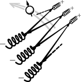
Figure 4: Penrose’s zig-zag electron, reimagined. (Cf. Fig. 25.1b of [91].)

Massive twistor diagrams?

Our explorations on the “diagrammar” of the massive twistor particle eventually extend to Hodges diagram [92, 93, 94, 95, 96, 97, 98, 99, 100, 101, 102, 103, 104, 105], which was indeed another inspiration behind the development of zig-zag diagrams.

Let us reimagine zig-zag diagrams in a Hodges-like notation. The implementation is again by Penrose graphical notation, but with the “differentiation balloon” of Penrose as well as birdtracks/trace diagram notations for the $\mathrm{SU}(2)$ epsilon tensor (see [90] and references therein). The basic elements are

$$Z_{\mathrm{A}}{}^{I}=\includegraphics[valign={c},scale={1.0}]{figs/hodges/dotZind.pdf}\,,\quad{\bar{Z}}_{I}{}^{\mathrm{A}}=\includegraphics[valign={c},scale={1.0}]{figs/hodges/dotZind-b.pdf}\,,\quad\epsilon_{IJ}=\includegraphics[valign={c},scale={1.0}]{figs/hodges/edown.pdf}\,,\quad\epsilon^{IJ}=\includegraphics[valign={c},scale={1.0}]{figs/hodges/eup.pdf}\,.$$ (183)

The difference in thickness distinguishes the vector spaces. Also, let us denote differential forms by “highlighted” dots:

$$dZ_{\mathrm{A}}{}^{I}=\includegraphics[valign={c},scale={1.0}]{figs/hodges/dZind.pdf}\,,\quad d{\bar{Z}}_{I}{}^{\mathrm{A}}=\includegraphics[valign={c},scale={1.0}]{figs/hodges/dZind-b.pdf}\,.$$ (184)

The free theory Poisson bivector $\omega^{\circ}{}^{-1}$ is suggestive of the Fourier transform between the twistor and dual twistor spaces, which is drawn like squiggly “propagators” in the Hodges notation. In this light, we denote

$$i\includegraphics[valign={c}]{figs/l.pdf}\includegraphics[valign={c}]{figs/r-b.pdf}\,\,\,\,\text{or}\,\,\,\,{-i}\includegraphics[valign={c}]{figs/l-b.pdf}\includegraphics[valign={c}]{figs/r.pdf}\quad\rightsquigarrow\quad\includegraphics[valign={c}]{figs/hodges/PBsquig.pdf}$$ (185)

so that

$$\frac{\partial}{\partial Z_{\mathrm{A}}{}^{I}}=\includegraphics[valign={c}]{figs/hodges/partialZind-b.pdf}\,,\qquad\frac{\partial}{\partial{\bar{Z}}_{I}{}^{\mathrm{A}}}=\includegraphics[valign={c}]{figs/hodges/partialZind.pdf}\,,\qquad\,\includegraphics[valign={c}]{figs/hodges/PBid-1.pdf}=\includegraphics[valign={c}]{figs/hodges/PBid-2.pdf}\,.$$ (186)

Now consider the self-dual plane wave symplectic perturbation for electromagnetism:

$$\omega^{\prime+}\hskip 1.00006pt=\hskip 1.00006pt-\frac{iq}{\sqrt{2}\Delta}\hskip 1.00006pt({\bar{\mathsf{3}}}_{\dot{{\gamma}}}\rho^{{\dot{{\gamma}}}{\mathrm{A}}})({\bar{\mathsf{3}}}_{\dot{{\delta}}}\rho^{{\dot{{\delta}}}{\mathrm{B}}})\hskip 0.50003pt(dZ_{\mathrm{A}}{}^{I}\wedge dZ_{\mathrm{B}}{}^{J})\hskip 1.00006pt\epsilon_{IJ}\,{\mathrm{e}}^{-i\hskip 0.35002pt{\bar{\mathsf{3}}}{z}{\mathsf{3}}}\,.$$ (187)

We can half-Fourier transform this into the photon’s dual twistor space, ${\bar{W}}^{A}=\big{(}-i\bar{\varpi}^{\alpha}\,\,\hskip 1.00006pt{\bar{\mathsf{3}}}_{\dot{\alpha}}\big{)}$:

$$\omega^{\prime+}\hskip 1.00006pt=\hskip 1.00006pt-\frac{iq}{\sqrt{2}\Delta}\hskip 1.00006pt({\bar{W}}^{\mathrm{A}}dZ_{\mathrm{A}}{}^{I}){\hskip 1.00006pt\wedge\hskip 1.00006pt}({\bar{W}}^{\mathrm{B}}dZ_{\mathrm{B}}{}^{J})\hskip 1.00006pt\epsilon_{IJ}\,\delta^{(2)}(\bar{\varpi}-{\bar{\mathsf{3}}}z)\,.$$ (188)

Curiously, the photon’s massless dual twistor is incident at the massive particle’s holomorphic position $z^{{\dot{\alpha}}\alpha}$. This hints that the photon’s propagator is also “zig-zag” in the field theory of Newman-Janis shifted fields in spin-space-time: Zwanziger electromagnetism [191, 192, 193, 194, 195]. Anyway, if the delta function is dropped for simplicity, (188) appears as

$$\omega^{\prime+}\hskip 1.00006pt=\hskip 1.00006pt-\frac{iq}{\sqrt{2}\Delta}\,\hskip 1.00006pt\includegraphics[valign={c}]{figs/hodges/Oem-1.pdf}\,.$$ (189)

In turn, the vector field $-\includegraphics[valign={c}]{figs/l-b.pdf}\includegraphics[valign={c}]{figs/v+.pdf}\includegraphics[valign={c}]{figs/xD-b.pdf}$ is graphically computed as

$$\begin{split}\frac{i\sqrt{2}q}{\Delta}\,\includegraphics[valign={c}]{figs/hodges/Oem-calc1.pdf}\,=\,\hskip 1.00006pt\frac{i\sqrt{2}q}{\Delta}\,\includegraphics[valign={c}]{figs/hodges/Oem-calc2.pdf}\,.\end{split}$$ (190)

Following [92], the infinity twistors are denoted as dashed lines.

While Guevara [14] has half-Fourier transformed the classical-spin amplitudes to the twistor space of the massless particle, it is tempting to have a description of the amplitudes that is fully twistorial for both massless and massive particles. In this context, it would be interesting to see if half-Fourier transformed symplectic perturbations and zig-zag vector fields can lead to a Hodges diagram for massive particles.

For over fifty years, twistor theory has provided a unique perspective on the physics of massless particles and fields in four dimensions. We hope that our zig-zag symplectic perturbation theory in the massive twistor space could signal the dawn of “massive twistor theory.”

Appendix A TBMT and MPTD equations

TBMT

The Thomas-Bargmann-Michel-Telegdi equation [41, 42, 43, 44, 45, 46] describes a spinning particle moving in a background electromagnetic field in special relativity. In this paper, by a massive spinning particle is governed by the TBMT equation with a certain $g$ value we mean that its momentum and spin length pseudovector obey the following equations in the covariant spin gauge with the gauge fixing $-p_{m}\hskip 0.50003pty^{m}=0$ of the residual redundancy:

$$\begin{split}0&{}\,=\,{}\dot{p}_{m}+p_{n}\hskip 1.00006pt\phi^{n}{}_{m}/m+\mathcal{O}(y^{1})\,,\\ 0&{}\,=\,{}\dot{y}^{m}-\frac{1}{m}\bigg{(}\hskip 1.00006pt{\frac{g}{2}\,\phi^{m}{}_{n}-\Big{(}1{\hskip 1.00006pt-\hskip 1.00006pt}\frac{g}{2}\hskip 1.00006pt\Big{)}\,\frac{\hskip 0.24994pt{p^{m}p_{l}}\hskip 0.24994pt}{m^{2}}\,\phi^{l}{}_{n}}\bigg{)}\hskip 1.00006pty^{n}+\mathcal{O}(y^{2})\,.\end{split}$$ (191)

$\phi_{mn}$ is an antisymmetric tensor. We use these terminologies “TBMT equation” and “$g$ factor” in a broad, general sense that does not restrict $\phi_{mn}$ to be the field strength of electromagnetism. For instance, it can be something depending on other dynamical variables of the spinning particle such as $q_{a}F^{a}{}_{mn}(x)$ of Yang-Mills or $2\hskip 0.50003ptp_{r}\gamma^{r}{}_{[mn]}(x)$ of gravity.

MPTD

The Mathisson-Papapetrou-Tulczyjew-Dixon equation [47, 48, 49, 50, 51, 52, 53, 54] describes the dynamics of a spinning particle in curved spacetime. It is extended by a parameter $\kappa$, which is called the “gravimagnetic ratio” in the literature [55, 56, 57, 58, 59, 60, 61]. Our version reads

$$\begin{split}0&{}\,=\,{}m\hskip 1.00006pte^{m}{}_{\mu}(x)\hskip 1.00006pt\dot{x}^{\mu}-p^{m}+\mathcal{O}(y^{1})\,,\\ 0&{}\,=\,{}\dot{p}_{m}-p_{n}\hskip 1.00006pt\gamma^{n}{}_{ms}(x)\hskip 1.00006pte^{s}{}_{\sigma}(x)\hskip 1.00006pt\dot{x}^{\sigma}-\frac{g}{2}\,p_{n}\hskip 1.00006pt{\star R}^{n}{}_{mrs}(x)\hskip 1.00006pty^{r}\hskip 0.50003pte^{s}{}_{\sigma}(x)\hskip 1.00006pt\dot{x}^{\sigma}+\mathcal{O}(y^{2})\,,\\ 0&{}\,=\,{}\dot{y}^{m}+\bigg{(}\hskip 1.00006pt{\frac{g}{2}\,\gamma^{m}{}_{ns}(x)-\Big{(}1{\hskip 1.00006pt-\hskip 1.00006pt}\frac{g}{2}\hskip 1.00006pt\Big{)}\,\frac{\hskip 0.24994pt{p^{m}p_{l}}\hskip 0.24994pt}{m^{2}}\,\gamma^{l}{}_{ns}(x)}\bigg{)}\hskip 1.00006pty^{n}\hskip 1.00006pte^{s}{}_{\sigma}(x)\hskip 1.00006pt\dot{x}^{\sigma}\\ &{}\phantom{{}\,=\,{}\dot{y}^{m}}{}+\bigg{(}\hskip 1.00006pt{\kappa\,{\star R}^{m}{}_{nrs}(x)-\Big{(}\hskip 0.50003pt\frac{g}{2}{\hskip 1.00006pt-\hskip 1.00006pt}\kappa\Big{)}\,\frac{\hskip 0.24994pt{p^{m}p_{l}}\hskip 0.24994pt}{m^{2}}\,{\star R}^{l}{}_{nrs}(x)}\bigg{)}\hskip 1.00006pty^{n}\hskip 1.00006pty^{r}\hskip 1.00006pte^{s}{}_{\sigma}(x)\hskip 1.00006pt\dot{x}^{\sigma}+\mathcal{O}(y^{3})\,,\end{split}$$ (192)

with the covariant gauge and the constraint $-p_{m}\hskip 0.50003pty^{m}=0$. $e^{m}{}_{\sigma}(x)$, $\gamma^{m}{}_{ns}(x)$, $R^{m}{}_{nrs}(x)$ denote the tetrad, spin connection coefficients, and Riemann tensor. As in (191), the momentum equation sets the “zero point” of non-minimal parameters: the precessions of $p_{m}$ and $y^{m}$ are synchronized when $1=g/2=\kappa$. By including $g$ in (192), we are being maximally pedantic, intending to maximally mimic the amplitude. Of course, it is fixed to $g{\,=\,}2$ by the general covariance of the spin vector: the spin vector should behave as the same as two infinitesimally deviated points. For more details, see Appendix B of [9].

Either of the two bracketed terms in the $\dot{y}^{m}$ equation can be viewed as a “double copy” of the bracketed term in (191). This is because there exist two ways of drawing analogies between electromagnetism/Yang-Mills and gravity. The first term, which defines the “gravitational gyromagnetic ratio” $g$, follows from (191) by taking $\phi_{mn}=-m\hskip 1.00006pt\gamma_{mn\rho}(x)\hskip 1.00006pt\dot{x}^{\rho}\,(\sim p_{r}\hskip 0.50003pt2\gamma^{r}{}_{[mn]}(x))$. Then one is comparing $A$ to $e^{m}$ and $F$ to $\gamma^{m}{}_{n}$ as in Kaluza-Klein reduction [196, 197, 198, 199, 200] or the gravitoelectromagnetism formulation of linearized gravity [201, 202, 203, 204, 205, 206, 207, 208, 209, 210, 211, 212, 213, 214, 215, 216, 217, 218], which realizes the “connection as field strength” argument in [82]. This parallel is suggested from the usual formulation of flat-space graviton scattering amplitudes in terms of metric perturbations and also from the “exact sequences of electromagnetism and gravity” diagram in [82]. More poetically, we could say “Aharanov-Bohm double copies to Sagnac” [219]: the Coriolis force is the gravitomagnetic force. On the other hand, the second term follows from (191) by taking $\phi_{mn}=-m\,{\star R}_{mnrs}(x)\hskip 1.00006pty^{r}\hskip 0.50003pte^{s}{}_{\sigma}(x)\hskip 1.00006pt\dot{x}^{\sigma}$ while putting $g{\hskip 1.00006pt=\hskip 1.00006pt}2$ and replacing $g/2$ with $\kappa$. Then one is comparing $A$ to $\gamma^{m}{}_{n}$ and $F$ to $R^{m}{}_{n}$. This way of thinking is more natural in a background independent/non-perturbative set-up and is encouraged by Ashtekar variables [220, 221, 222, 223, 224, 225, 226], non-linear graviton [157, 156], Weyl double copy [227, 228, 229, 230], covariant color-kinematics duality [231], etc.

Both of these two parallels emerge in our discussion on the symplectic perturbation theory of spinning particles: the former from the non-covariant scheme employed in this paper and the latter from the covariant scheme employed in the follow-up paper [83].

Generic $\mathcal{O}(\phi^{1})$ spin precession equation of motion

In this paper, we have proposed a generic spin precession equation of motion, all orders in spin and first order in the formal “field strength” $\phi$. When $\phi$ is self-dual, it reads

$$\begin{split}0&{}\,=\,{}\dot{p}_{m}+\frac{1}{m}\,p_{n}\Bigg{[}\hskip 1.00006pt{\sum_{\ell=0}^{\infty}\hskip 1.00006pt\frac{(C_{\ell}{\hskip 1.00006pt+\hskip 1.00006pt}\tilde{C}_{\ell}\hskip 1.00006pt\star^{-1})}{\ell!}\hskip 1.00006pt\big{(}{(y{\hskip 1.00006pt\cdot\hskip 1.00006pt}\partial)^{\ell}\hskip 1.00006pt{\star^{\ell}\phi}(x)}\big{)}{}^{n}{}_{m}}\Bigg{]}\hskip 1.00006pt+\hskip 1.00006pt\mathcal{O}(\phi^{2})\,,\\ 0&{}\,=\,{}\dot{y}^{m}-\frac{1}{m}\left[{\begin{array}[]{l}\displaystyle\sum_{\ell=0}^{\infty}\frac{(C_{\ell+1}{\hskip 1.00006pt+\hskip 1.00006pt}\tilde{C}_{\ell+1}\hskip 1.00006pt\star^{-1})}{\ell!}\hskip 1.00006pt\big{(}{(y{\hskip 1.00006pt\cdot\hskip 1.00006pt}\partial)^{\ell}\hskip 1.00006pt{\star^{\ell}\phi}(x)}\big{)}{}^{m}{}_{n}\\ \displaystyle{}-\frac{p^{m}p_{r}}{m^{2}}\hskip 1.00006pt\sum_{\ell=0}^{\infty}\frac{(C_{\ell}{\hskip 1.00006pt+\hskip 1.00006pt}\tilde{C}_{\ell}\hskip 1.00006pt\star^{-1})-(C_{\ell+1}{\hskip 1.00006pt+\hskip 1.00006pt}\tilde{C}_{\ell+1}\hskip 1.00006pt\star^{-1})}{\ell!}\hskip 1.00006pt\big{(}{(y{\hskip 1.00006pt\cdot\hskip 1.00006pt}\partial)^{\ell}\hskip 1.00006pt{\star^{\ell}\phi}(x)}\big{)}{}^{r}{}_{n}\end{array}}\right]y^{n}\\ &\quad\hskip 1.00006pt+\hskip 1.00006pt\mathcal{O}(\phi^{2})\,,\end{split}$$ (193)

where we have also included magnetic Wilson coefficients $\tilde{C}_{\ell}$ for full generality. One obtains (191) and (192) by truncating (193) with having $C_{1}{\,=\,}g/2$, $C_{2}{\,=\,}\kappa$, and $\tilde{C}_{\ell}{\,=\,}0$.

As pointed out recently in [2], $\dot{p}_{m}$ and $\dot{y}^{m}$ can be described together in a more unified manner in terms of the spin frames as $\dot{\lambda}{}_{\alpha}{}^{I}$, $\dot{{\bar{\lambda}}}{}_{I{\dot{\alpha}}}$. This is best illustrated if the body-frame components of the spin pseudovector are constant, which happens in our setting when the particle has a constant Regge trajectory. The spin frame version of (193) reads

$$\begin{split}m_{0}\hskip 1.00006pt\dot{{\bar{\lambda}}}{}_{I{\dot{\alpha}}}&{}\,=\,{}{\bar{\lambda}}_{\smash{I{\dot{\beta}}}\vphantom{I{\dot{\alpha}}}}\hskip 1.00006pt\Bigg{[}\hskip 1.00006pt{\sum_{\ell=0}^{\infty}\hskip 1.00006pt\frac{1}{\hskip 0.24994pt\ell!\hskip 0.24994pt}\frac{C^{+}_{\ell}{\hskip 1.00006pt+\hskip 1.00006pt}C^{+}_{\ell+1}}{2}\hskip 1.00006pt(iy{\hskip 1.00006pt\cdot\hskip 1.00006pt}\partial)^{\ell}\phi^{\dot{\beta}}{}_{\dot{\alpha}}(x)}\Bigg{]}\hskip 1.00006pt+\hskip 1.00006pt\mathcal{O}(\phi^{2})\,,\\ m_{0}\hskip 1.00006pt\dot{\lambda}{}_{\alpha}{}^{I}&{}\,=\,{}\lambda_{\alpha}{}^{J}\hskip 1.00006pt\hskip 1.00006pt{\bar{\lambda}}_{\smash{J{\dot{\beta}}}\vphantom{I{\dot{\alpha}}}}\Bigg{[}\hskip 1.00006pt{\sum_{\ell=0}^{\infty}\hskip 1.00006pt\frac{1}{\hskip 0.24994pt\ell!\hskip 0.24994pt}\frac{C^{+}_{\ell}{\hskip 1.00006pt-\hskip 1.00006pt}C^{+}_{\ell+1}}{2}\hskip 1.00006pt(iy{\hskip 1.00006pt\cdot\hskip 1.00006pt}\partial)^{\ell}\phi^{\dot{\beta}}{}_{\dot{\alpha}}(x)}\Bigg{]}({\bar{\lambda}}^{-1})^{{\dot{\alpha}}I}\hskip 1.00006pt+\hskip 1.00006pt\mathcal{O}(\phi^{2})\,,\end{split}$$ (194)

where $C^{\pm}_{\ell}=C_{\ell}{\,\mp\,}i\hskip 0.50003pt\tilde{C}_{\ell}$. One can clearly see that $\dot{\lambda}{}_{\alpha}{}^{I}=0+\mathcal{O}(\phi^{2})$ in self-dual backgrounds implies $C^{+}_{\ell}{\,=\,}C^{+}_{0}{\,=\,}1$ and vice versa: all three-point spin multipole couplings (not only dipole and quadrupole, to emphasize) to the self-dual field are Kerr-Newman.

These equations were already implied throughout (68), (69), (78), (88), (89), but we have restated them in terms of the real-worldline Wilson coefficients for reference.

Lastly, we spell out the spin frame versions of (191) and (192):

$$\begin{split}\dot{{\bar{\lambda}}}{}_{I{\dot{\alpha}}}&{}\hskip 1.00006pt=\hskip 1.00006pt\textstyle\frac{1+g/2}{2}\,\hskip 0.50003pt{\bar{\lambda}}_{\smash{I{\dot{\beta}}}\vphantom{I{\dot{\alpha}}}}\hskip 1.00006pt\hskip 1.00006pt\phi^{\dot{\beta}}{}_{\dot{\alpha}}(x)/m_{0}+\mathcal{O}(y^{1})\,,\\ \dot{\lambda}{}_{\alpha}{}^{I}&{}\hskip 1.00006pt=\hskip 1.00006pt\textstyle\frac{1-g/2}{2}\,\hskip 0.50003pt\lambda_{\alpha}{}^{J}\,{\bar{\lambda}}_{\smash{J{\dot{\beta}}}\vphantom{I{\dot{\alpha}}}}\hskip 1.00006pt\phi^{\dot{\beta}}{}_{\dot{\alpha}}(x)\hskip 0.24994pt({\bar{\lambda}}^{-1})^{{\dot{\alpha}}I}/m_{0}+\mathcal{O}(y^{1})\,,\end{split}$$ (195)

$$\begin{split}\dot{{\bar{\lambda}}}{}_{I{\dot{\alpha}}}&{}\hskip 1.00006pt=\hskip 1.00006pt\textstyle-{\bar{\lambda}}_{\smash{I{\dot{\beta}}}\vphantom{I{\dot{\alpha}}}}\hskip 1.00006pt\Big{[}\hskip 0.50003pt{\frac{1+g/2}{2}\hskip 1.00006pt\hskip 0.24994pt\gamma^{\dot{\beta}}{}_{{\dot{\alpha}}s}(x)+\frac{g/2+\kappa}{2}\hskip 0.50003ptR^{\dot{\beta}}{}_{{\dot{\alpha}}rs}(x)\hskip 1.00006pty^{r}+\mathcal{O}(y^{2})}\hskip 0.24994pt\Big{]}\,e^{s}{}_{\sigma}(x)\hskip 1.00006pt\dot{x}^{\sigma}\,,\\[-0.86108pt] \dot{\lambda}{}_{\alpha}{}^{I}&{}\hskip 1.00006pt=\hskip 1.00006pt\textstyle-\lambda_{\alpha}{}^{J}\,{\bar{\lambda}}_{\smash{J{\dot{\beta}}}\vphantom{I{\dot{\alpha}}}}\hskip 1.00006pt\Big{[}\hskip 0.50003pt{\frac{1-g/2}{2}\hskip 1.00006pt\hskip 0.24994pt\gamma^{\dot{\beta}}{}_{{\dot{\alpha}}s}(x)+\frac{g/2-\kappa}{2}\hskip 0.50003ptR^{\dot{\beta}}{}_{{\dot{\alpha}}rs}(x)\hskip 1.00006pty^{r}+\mathcal{O}(y^{2})}\hskip 0.24994pt\Big{]}({\bar{\lambda}}^{-1})^{{\dot{\alpha}}I}\,e^{s}{}_{\sigma}(x)\hskip 1.00006pt\dot{x}^{\sigma}\,,\end{split}$$ (196)

Appendix B Matching Calculation

Classical spin from coherent states

Aoude and Ochirov [10] have explicated the procedure of obtaining massive spinning amplitudes in the classical spin limit in terms of spin coherent states. We briefly review their methodology in our notation. See also [17] for a succinct review.

Modeling the spinning degrees of freedom by the coadjoint orbit [235, 236, 237, 238, 239], the classical value of spin angular momentum is identified with its coherent-state expectation value in the first-quantized theory as

$$W_{a}=(\hbar/2)\hskip 1.00006pt{\smash{\bar{\psi}}\kern 0.20004pt\vphantom{\psi}}^{I}(\sigma_{a})_{I}{}^{J}\psi_{J}\,,\quad|\vec{W}|=(\hbar/2)\hskip 1.00006pt{\smash{\bar{\psi}}\kern 0.20004pt\vphantom{\psi}}^{I}\psi_{I}\,.$$ (197)

The classical-spin amplitude then follows from the coherent-state expectation value of all definite-spin amplitudes in the $\hbar\to 0$ limit with $|\vec{W}|$ fixed:

$$\begin{split}\mathcal{M}({\mathsf{1}},a;{\mathsf{3}}){\phantom{{}:={}}\mathllap{{}={}}}{}&\lim_{\begin{subarray}{c}\hbar\to 0\\ {\smash{\bar{\psi}}\kern 0.14003pt\vphantom{\psi}}\psi=2|\vec{W}|/\hbar\end{subarray}}\sum_{2s=0}^{\infty}\mathcal{M}_{(2s)}({\mathsf{1}},{\smash{\bar{\psi}}\kern 0.20004pt\vphantom{\psi}},\psi;{\mathsf{3}})\,,\\ \mathcal{M}_{(2s)}({\mathsf{1}},{\smash{\bar{\psi}}\kern 0.20004pt\vphantom{\psi}},\psi;{\mathsf{3}}):={}&\frac{{\mathrm{e}}^{-{\smash{\bar{\psi}}\kern 0.14003pt\vphantom{\psi}}\psi}}{(2s)!}\,\hskip 1.00006pt{\smash{\bar{\psi}}\kern 0.20004pt\vphantom{\psi}}^{J_{1}}\cdots{\smash{\bar{\psi}}\kern 0.20004pt\vphantom{\psi}}^{J_{2s}}\hskip 1.00006pt(\mathcal{A}_{(2s)}({\mathsf{2}}{\leftarrow}{\mathsf{1}};{\mathsf{3}}))_{J_{1}\cdots J_{2s}}{}^{I_{1}\cdots I_{2s}}\,\psi_{I_{1}}\cdots\psi_{I_{2s}}\,,\end{split}$$ (198)

where ${\mathrm{e}}^{-{\smash{\bar{\psi}}\kern 0.14003pt\vphantom{\psi}}\psi}$ is the measure normalizing coherent states. For example, the spin-tensor ${\hbox to0.0pt{1\hss}\hskip 1.6pt\resizebox{}{}{\scalebox{1.1}[1.1]{{\leavevmode\hbox{\set@color{1}}}}}}^{\odot 2s}$ of the plus-helicity minimal amplitude $\smash{\mathcal{A}^{+h}_{(2s)}({\mathsf{2}}{\leftarrow}{\mathsf{1}};{\mathsf{3}})=e_{h}\hskip 0.50003ptm_{0}x^{h}\hskip 1.00006pt{\hbox to0.0pt{1\hss}\hskip 1.6pt\resizebox{}{}{\scalebox{1.1}[1.1]{{\leavevmode\hbox{\set@color{1}}}}}}^{\odot 2s}}$ boils down to

$$\begin{split}{\mathrm{e}}^{-{\smash{\bar{\psi}}\kern 0.14003pt\vphantom{\psi}}\psi}\exp\Big{(}{\smash{\bar{\psi}}\kern 0.20004pt\vphantom{\psi}}^{J}\langle{\mathsf{2}}^{-1}_{J}{\mathsf{1}}^{I}\rangle\psi_{I}\Big{)}\hskip 1.00006pt=\hskip 1.00006pt{\mathrm{e}}^{{\mathsf{3}}\cdot a}\,,\end{split}$$ (199)

upon plugging in the real on-shell kinematics given in (92) [7, 10]. Note that

$$\begin{split}\langle{\mathsf{2}}^{-1}_{J}{\mathsf{1}}^{I}\rangle&=\delta_{J}{}^{I}-{\textstyle\frac{1}{2}}\hskip 0.50003pt\langle{\mathsf{1}}^{-1}_{I}{\mathsf{3}}\rangle{\kern-0.37003pt\leavevmode\hbox{$\vbox{\hbox{\resizebox{}{}{\scalebox{0.99}[0.99]{{\leavevmode\hbox{\set@color{${\lfloor\hbox to0.0pt{\hss\reflectbox{\rotatebox[origin={c}]{180.0}{$\lfloor$}}}}$}}}}}}}$}\kern-0.39993pt}{\bar{\mathsf{3}}}{\bar{\mathsf{1}}}^{-1}{}^{J}{\kern-0.39993pt\leavevmode\hbox{$\vbox{\hbox{\resizebox{}{}{\scalebox{0.99}[0.99]{{\leavevmode\hbox{\set@color{${\hbox to0.0pt{\reflectbox{\rotatebox[origin={c}]{180.0}{$\rfloor$}}\hss}\rfloor}$}}}}}}}$}\kern-0.37003pt}\,,\\ &=\delta_{J}{}^{I}+{\mathsf{3}}_{m}\Big{(}{\textstyle\frac{\hbar}{2m_{0}}\hskip 0.50003pt(\Lambda({\mathsf{1}}))^{m}{}_{a}\hskip 0.50003pt(\sigma^{a})_{I}{}^{J}+\frac{1}{2}\hskip 0.50003pt({\mathsf{1}}^{-1})^{m}\hskip 0.50003pt\delta_{I}{}^{J}}\kern-0.20004pt\Big{)}\,,\\ &=\delta_{J}{}^{I}+{\textstyle\frac{\hbar}{2m_{0}}}\hskip 1.00006pt{\mathsf{3}}_{m}(\Lambda({\mathsf{1}}))^{m}{}_{a}\hskip 0.50003pt(\sigma^{a})_{I}{}^{J}\end{split}$$ (200)

on the support of $\delta\kern-1.99997pt\makebox[0.0pt][l]{$\bar{}$}\kern 1.99997pt(2\hskip 1.00006pt{\mathsf{1}}{\hskip 1.00006pt\cdot\hskip 1.00006pt}{\mathsf{3}})$. In turn, it follows that

$${\smash{\bar{\psi}}\kern 0.20004pt\vphantom{\psi}}^{J}\langle{\mathsf{2}}^{-1}_{J}{\mathsf{1}}^{I}\rangle\psi_{I}-{\smash{\bar{\psi}}\kern 0.20004pt\vphantom{\psi}}^{I}\psi_{I}\hskip 1.00006pt=\hskip 1.00006pt{\mathsf{3}}{\hskip 1.00006pt\cdot\hskip 1.00006pt}a({\mathsf{1}})\,.$$ (201)

In our spherical top setting, such classical-spin states are realized in the $(\lambda,{\bar{\lambda}})$ polarization as polynomials of $\lambda_{\alpha}{}^{I}$ and $({\bar{\lambda}}^{-1})^{{\dot{\alpha}}I}$ saturated by a common spinor $\psi_{I}$; i.e., they are the “right” coherent states with respect to the $\mathrm{SU}(2)$ group action on $\mathbb{MA}$. The unoccupied “left” $\mathrm{SL}(2,\mathbb{C})$ indices contract to amplitudes as spacetime spinor-tensors.

Matching

Applying (198) with the real kinematics (92), the coherent-state expectation value of the plus-helicity spinning amplitude (107a) is given as

$$\begin{split}&\phantom{=}\,\,\hskip 1.00006pt\hskip 1.00006pt\hskip 0.50003pte_{h}\hskip 0.50003ptm_{0}x^{h}\hskip 1.00006pt{\mathrm{e}}^{-{\smash{\bar{\psi}}\kern 0.14003pt\vphantom{\psi}}\psi}\hskip 1.00006pt\sum_{2s=0}^{\infty}\sum_{\ell=0}^{2s}\frac{\hskip 0.50003ptg^{+}_{\ell}\hbar^{\ell}\hskip 0.50003pt}{(2s)!}\hskip 1.00006pt\big{(}{\smash{\bar{\psi}}\kern 0.20004pt\vphantom{\psi}}\psi+{\mathsf{3}}{\hskip 1.00006pt\cdot\hskip 1.00006pt}a\big{)}^{2s-\ell}(-2\hskip 1.00006pt{\mathsf{3}}{\hskip 1.00006pt\cdot\hskip 1.00006pt}a)^{\ell}\,,\\ &=e_{h}\hskip 0.50003ptm_{0}x^{h}\hskip 1.00006pt{\mathrm{e}}^{-{\smash{\bar{\psi}}\kern 0.14003pt\vphantom{\psi}}\psi}\hskip 1.00006pt\sum_{\ell=0}^{\infty}\hskip 1.00006ptg^{+}_{\ell}\hbar^{\ell}\left(\frac{-2\hskip 1.00006pt{\mathsf{3}}{\hskip 1.00006pt\cdot\hskip 1.00006pt}a}{\vphantom{\leavevmode\hbox{\raise 1.99997pt\hbox{\set@color\resizebox{}{}{{\leavevmode\hbox{\set@color{${\smash{\bar{\psi}}\kern 0.20004pt\vphantom{\psi}}$}}}}}}}{\smash{\bar{\psi}}\kern 0.20004pt\vphantom{\psi}}\psi+{\mathsf{3}}{\hskip 1.00006pt\cdot\hskip 1.00006pt}a}\right)^{\kern-1.18999pt\ell}\sum_{2s=\ell}^{\infty}\frac{1}{(2s)!}\hskip 0.50003pt\big{(}{\smash{\bar{\psi}}\kern 0.20004pt\vphantom{\psi}}\psi+{\mathsf{3}}{\hskip 1.00006pt\cdot\hskip 1.00006pt}a\big{)}^{2s}\,,\\ &=e_{h}\hskip 0.50003ptm_{0}x^{h}\hskip 1.00006pt{\mathrm{e}}^{{\mathsf{3}}\cdot a}\hskip 1.00006pt\sum_{\ell=0}^{\infty}\hskip 1.00006ptg^{+}_{\ell}\hbar^{\ell}\left(\frac{-2\hskip 1.00006pt{\mathsf{3}}{\hskip 1.00006pt\cdot\hskip 1.00006pt}a}{\vphantom{\leavevmode\hbox{\raise 1.99997pt\hbox{\set@color\resizebox{}{}{{\leavevmode\hbox{\set@color{${\smash{\bar{\psi}}\kern 0.20004pt\vphantom{\psi}}$}}}}}}}{\smash{\bar{\psi}}\kern 0.20004pt\vphantom{\psi}}\psi+{\mathsf{3}}{\hskip 1.00006pt\cdot\hskip 1.00006pt}a}\right)^{\kern-1.18999pt\ell}\left(1-\frac{1}{(\ell-1)!}\hskip 1.00006pt\Gamma\big{(}\ell\hskip 0.50003pt\big{|}\hskip 0.50003pt{\smash{\bar{\psi}}\kern 0.20004pt\vphantom{\psi}}\psi+{\mathsf{3}}{\hskip 1.00006pt\cdot\hskip 1.00006pt}a\big{)}\kern-0.15pt\right)\,.\end{split}$$ (202)

As argued in [10] around equations (3.22)-(3.27), for large ${\smash{\bar{\psi}}\kern 0.20004pt\vphantom{\psi}}\psi$ this has the limit

$$\begin{split}&\mathcal{M}^{+h}[g^{+}](x,a;{\mathsf{3}})=e_{h}\hskip 0.50003ptm_{0}x^{h}\hskip 1.00006pt{\mathrm{e}}^{{\mathsf{3}}\cdot a}\left(\lim_{\hbar\to 0}\hskip 1.00006pt\sum_{\ell=0}^{\infty}\hskip 1.00006ptg^{+}_{\ell}\hbar^{\ell}\hskip 1.00006pt\bigg{(}{-\frac{{\mathsf{3}}{\hskip 1.00006pt\cdot\hskip 1.00006pt}a}{\hskip 0.50003pt|\vec{W}|/\hbar\hskip 0.50003pt}}\bigg{)}^{\kern-1.18999pt\ell}\,\right)\,.\end{split}$$ (203)

Therefore, provided that $g^{+}_{\ell}$ scales as $\mathcal{O}(\hbar^{-\ell})$, we conclude that

$$f^{+}_{\ell}=(-|\vec{W}|)^{-\ell}\cdot\lim_{\hbar\to 0}g^{+}_{\ell}\hbar^{\ell}{\quad\implies\quad}f^{+}(\xi)=g^{+}(-\xi/|\vec{W}|)$$ (204)

by comparing (LABEL:eq:M+coherent) with $\mathcal{M}^{+h}[f^{+}]({\mathsf{1}},a;{\mathsf{3}})=\mathcal{M}^{+h}({\mathsf{1}},a;{\mathsf{3}})\,{\cdot}\,f^{+}({\mathsf{3}}{\hskip 1.00006pt\cdot\hskip 1.00006pt}a)$ of (104).

A trick

Lastly, we demonstrate a slightly quicker derivation. As shown in (199), the real kinematics (92) has induced the minimal exponential spin factor ${\mathrm{e}}^{{\mathsf{3}}\cdot a}$. However, we find that we can either apply the complexified kinematics (94c) and put ${\mathrm{e}}^{{\mathsf{3}}\cdot a}$ by hand. For minimal coupling, it works as

$$\begin{split}{\mathsf{1}}_{\alpha}{}^{I}=\hskip 1.00006pt{\mathsf{2}}_{\alpha}{}^{I}{\quad\implies\quad}{\mathcal{M}}({\mathsf{1}},a;{\mathsf{3}})\hskip 1.00006pt&=\hskip 1.00006pte_{h}\hskip 0.50003ptm_{0}x^{h}\hskip 1.00006pte^{{\mathsf{3}}\cdot a}\left({\mathrm{e}}^{-{\smash{\bar{\psi}}\kern 0.14003pt\vphantom{\psi}}\psi}\exp\Big{(}{\smash{\bar{\psi}}\kern 0.20004pt\vphantom{\psi}}^{J}\langle{\mathsf{2}}^{-1}_{J}{\mathsf{1}}^{I}\rangle\psi_{I}\Big{)}\right)\,,\\ \hskip 1.00006pt&=\hskip 1.00006pte_{h}\hskip 0.50003ptm_{0}x^{h}\hskip 1.00006pte^{{\mathsf{3}}\cdot a}\,.\end{split}$$ (205)

This trick may be thought of as an analog of taking the holomorphic complex worldline as the “zero point”: the Newman-Janis shifted amplitude is taken as default. One can check that it also works in the non-minimal case:

$$\begin{split}&\phantom{=}\,\,\hskip 1.00006pt\hskip 1.00006pt\hskip 0.50003pt{\mathrm{e}}^{{\mathsf{3}}\cdot a}\left(e_{h}\hskip 0.50003ptm_{0}x^{h}\hskip 1.00006pt{\mathrm{e}}^{-{\smash{\bar{\psi}}\kern 0.14003pt\vphantom{\psi}}\psi}\hskip 1.00006pt\sum_{2s=0}^{\infty}\sum_{\ell=0}^{2s}\frac{\hskip 0.50003ptg^{+}_{\ell}\hbar^{\ell}\hskip 0.50003pt}{(2s)!}\hskip 1.00006pt({\smash{\bar{\psi}}\kern 0.20004pt\vphantom{\psi}}\psi)^{2s-\ell}(-2\hskip 1.00006pt{\mathsf{3}}{\hskip 1.00006pt\cdot\hskip 1.00006pt}a)^{\ell}\right)\,,\\ &={\mathrm{e}}^{{\mathsf{3}}\cdot a}\left(e_{h}\hskip 0.50003ptm_{0}x^{h}\hskip 1.00006pt\sum_{\ell=0}^{\infty}\hskip 1.00006ptg^{+}_{\ell}\hbar^{\ell}\left(\frac{-2\hskip 1.00006pt{\mathsf{3}}{\hskip 1.00006pt\cdot\hskip 1.00006pt}a}{\vphantom{\leavevmode\hbox{\raise 1.99997pt\hbox{\set@color\resizebox{}{}{{\leavevmode\hbox{\set@color{${\smash{\bar{\psi}}\kern 0.20004pt\vphantom{\psi}}$}}}}}}}{\smash{\bar{\psi}}\kern 0.20004pt\vphantom{\psi}}\psi}\right)^{\kern-1.18999pt\ell}\left(1-\frac{1}{(\ell-1)!}\hskip 1.00006pt\Gamma\big{(}\ell\hskip 0.50003pt\big{|}\hskip 0.50003pt{\smash{\bar{\psi}}\kern 0.20004pt\vphantom{\psi}}\psi+{\mathsf{3}}{\hskip 1.00006pt\cdot\hskip 1.00006pt}a\big{)}\kern-0.15pt\right)\right)\,.\end{split}$$ (206)

We have plugged in (94c) to (107a) and then placed ${\mathrm{e}}^{{\mathsf{3}}\cdot a}$ in front of it by hand while omitting $e_{h}\hskip 0.50003ptm_{0}x^{h}\hskip 1.00006pt$ to avoid clutter. In the large ${\smash{\bar{\psi}}\kern 0.20004pt\vphantom{\psi}}\psi$ limit, this agrees with the last line of (LABEL:eq:M+2scontrib) so that (LABEL:eq:M+coherent)-(204) are reproduced.

It is not difficult to understand why this trick works at the level of computation. For a deeper reason, it might be plausible to relate it to the fact that the quantum amplitude of the minimally coupled particle, derived in (214), is supported on ${\mathsf{1}}_{\alpha}{}^{I}={\mathsf{2}}_{\alpha}{}^{I}$.

Appendix C Hamiltonian Perturbation Theory

Finally, we would like to comment that it is also possible to develop the textbook perturbation theory (which perturbs the Hamiltonian, not the symplectic structure) for the massive twistor particle. The purpose of this digression is to complement our symplectic perturbation approach and point out possibilities of future applications, e.g., applying the KMO’C formalism [13]. We only demonstrate the simplest example: scattering of a minimally coupled fixed-mass particle in the plus-helicity electromagnetic plane wave.

Canonical quantization

We first-quantize the massive twistor particle in the reparameterization gauge (24) where the Hamiltonian is $H={\textstyle\frac{1}{-2}}({\bar{\Delta}}{\hskip 1.00006pt+\hskip 1.00006pt}\Delta)+m_{0}$ and treat it as a standard quantum-mechanical system with “absolute time.” In order to perform canonical quantization, one should figure out what the canonical coordinates are. A holomorphic electromagnetic field $A_{\alpha{\dot{\alpha}}}(z)\hskip 1.00006ptdz^{{\dot{\alpha}}\alpha}$ translates to $-i\hskip 0.50003pt(\lambda^{-1})_{I}{}^{\alpha}A_{\smash{\alpha{\dot{{\gamma}}}}\vphantom{{\dot{\alpha}}}}(z)\hskip 1.00006pt\rho^{{\dot{{\gamma}}}{\mathrm{A}}}\hskip 0.50003ptdZ_{\mathrm{A}}{}^{I}$ in the notation (50). Taking $i\hskip 1.00006pt{\bar{Z}}_{I}{}^{\mathrm{A}}dZ_{\mathrm{A}}{}^{I}$ for the free-theory symplectic potential, we find that the “kinetic” and “canonical” twistor variables are related as

$$(Z^{\text{kin}})_{\mathrm{A}}{}^{I}\hskip 1.00006pt=\hskip 1.00006pt(Z^{\text{can}})_{\mathrm{A}}{}^{I}\,,\quad({\bar{Z}}^{\text{kin}})_{I}{}^{\mathrm{A}}\hskip 1.00006pt=\hskip 1.00006pt({\bar{Z}}^{\text{can}})_{I}{}^{\mathrm{A}}\hskip 1.00006pt+\hskip 1.00006ptq(\lambda^{\text{kin}}{}^{-1})_{I}{}^{\alpha}\hskip 1.00006ptA_{\smash{\alpha{\dot{{\gamma}}}}\vphantom{{\dot{\alpha}}}}(z^{\text{kin}})\,(\rho^{\text{kin}})^{{\dot{{\gamma}}}{\mathrm{A}}}\,.$$ (207)

From now, we exclusively work with the canonical variables (unlike in the main text) and drop the “can” subscript to avoid clutter. Then (207) boils down to

$$\begin{split}\lambda_{\alpha}{}^{I}&=(\lambda^{\text{kin}})_{\alpha}{}^{I}\,,\quad\mu^{{\dot{\alpha}}I}=(\mu^{\text{kin}})^{{\dot{\alpha}}I}\,,\\ {\bar{\lambda}}_{I{\dot{\alpha}}}&=({\bar{\lambda}}^{\text{kin}})_{I{\dot{\alpha}}}-q(\lambda^{-1})_{I}{}^{\beta}A_{\smash{\beta{\dot{\alpha}}}\vphantom{{\dot{\alpha}}}}(z)\,,\\ {\bar{\mu}}_{I}{}^{\alpha}&=({\bar{\mu}}^{\text{kin}})_{I}{}^{\alpha}-q(\lambda^{-1})_{I}{}^{\beta}A_{\smash{\beta{\dot{\alpha}}}\vphantom{{\dot{\alpha}}}}(z)\hskip 1.00006ptz^{{\dot{\alpha}}\alpha}\,.\end{split}$$ (208)

While $z^{{\dot{\alpha}}\alpha}{\hskip 1.00006pt=\hskip 1.00006pt}(\mu\lambda^{-1})^{{\dot{\alpha}}\alpha}{\hskip 1.00006pt=\hskip 1.00006pt}(z^{\text{kin}})^{{\dot{\alpha}}\alpha}$, ${\bar{z}}^{{\dot{\alpha}}\alpha}{\hskip 1.00006pt=\hskip 1.00006pt}({\bar{\lambda}}^{-1}{\bar{\mu}})^{{\dot{\alpha}}\alpha}$ differs from $({\bar{z}}^{\text{kin}})^{{\dot{\alpha}}\alpha}$ due to coupling to the holomorphic gauge field.

The Hamiltonian $H={\textstyle\frac{1}{-2}}({\rm det}({\bar{\lambda}}^{\text{kin}}){\hskip 1.00006pt+\hskip 1.00006pt}{\rm det}(\lambda^{\text{kin}}))$ gets perturbed in this canonical setting as $H=H^{\circ}+H^{\prime}$, where $H^{\circ}={\textstyle\frac{1}{-2}}({\rm det}({\bar{\lambda}})+{\rm det}(\lambda))+m_{0}$ and $H^{\prime}=H^{\prime}_{1}+H^{\prime}_{2}$:

$$H^{\prime}_{1}:=\frac{\hskip 0.50003pt{\bar{\Delta}}\hskip 0.50003pt}{2}\hskip 1.00006ptqA_{\smash{\beta{\dot{\beta}}}\vphantom{{\dot{\alpha}}}}(z)\hskip 1.00006pt(p{}^{-1})^{{\dot{\beta}}\beta}\,,\quad H^{\prime}_{2}:=-\frac{1}{4\Delta}\hskip 1.00006ptq^{2}\hskip 1.00006pt\epsilon^{\alpha\beta}A_{\alpha{\dot{\alpha}}}(z)\hskip 1.00006ptA_{\smash{\beta{\dot{\beta}}}\vphantom{{\dot{\alpha}}}}(z)\hskip 1.00006pt{\bar{\epsilon}}^{{\dot{\alpha}}{\dot{\beta}}}\,.$$ (209)

We restrict our attention to the leading order and discard $H^{\prime}_{2}$. For the self-dual plane wave (116), the $\mathcal{O}(q^{1})$ interaction Hamiltonian becomes

$$H^{\prime}_{1}=\frac{q}{\sqrt{2}\Delta}\hskip 1.00006pt\langle\iota|p|{\bar{o}}{\kern-0.39993pt\leavevmode\hbox{$\vbox{\hbox{\resizebox{}{}{\scalebox{0.99}[0.99]{{\leavevmode\hbox{\set@color{${\hbox to0.0pt{\reflectbox{\rotatebox[origin={c}]{180.0}{$\rfloor$}}\hss}\rfloor}$}}}}}}}$}\kern-0.37003pt}\,{\mathrm{e}}^{-i\hskip 0.70004pt{\bar{o}}\mu\lambda^{-1}o}\,.$$ (210)

There are many kinds of eigenstates in the free theory that we can consider: coherent states ${\big{\langle}{{\bar{Z}}}\hskip 0.50003pt\big{|}\hskip 0.50003pt}$ and ${\hskip 0.50003pt\big{|}\hskip 0.50003pt{Z}\big{\rangle}}$, frame eigenstates ${\hskip 0.50003pt\big{|}\hskip 0.50003pt{\lambda{\bar{\lambda}}}\big{\rangle}}$, and simultaneous eigenstates of $\hat{p}_{\alpha{\dot{\alpha}}}$ and $\hat{\vec{W}}{}^{2}$, which might be called “Wigner states.” For our scattering problem, we identify ${\hskip 0.50003pt\big{|}\hskip 0.50003pt{\lambda{\bar{\lambda}}}\big{\rangle}}$ as the relevant in-state. Using the convention $\{Z_{\mathrm{A}}{}^{I},{\bar{Z}}_{J}{}^{\mathrm{B}}\}=(1/{i\hbar})\hskip 1.00006pt\delta_{\mathrm{A}}{}^{\mathrm{B}}\delta_{J}{}^{I}$ $\implies$ $\smash{[\hat{Z}_{\mathrm{A}}{}^{I},\hat{{\bar{Z}}}_{J}{}^{\mathrm{B}}]}=\delta_{\mathrm{A}}{}^{\mathrm{B}}\delta_{J}{}^{I}$ (see footnote 10), the canonically quantized operators are realized as

$$\begin{split}{\big{\langle}{\lambda{\bar{\lambda}}}\hskip 0.50003pt\big{|}\hskip 0.50003pt}\hskip 0.50003pt\hat{\lambda}_{\alpha}{}^{I}=\lambda_{\alpha}{}^{I}{\big{\langle}{\lambda{\bar{\lambda}}}\hskip 0.50003pt\big{|}\hskip 0.50003pt}&\,,\quad{\big{\langle}{\lambda{\bar{\lambda}}}\hskip 0.50003pt\big{|}\hskip 0.50003pt}\hskip 0.50003pt\hat{{\bar{\lambda}}}_{I{\dot{\alpha}}}={\bar{\lambda}}_{I{\dot{\alpha}}}{\big{\langle}{\lambda{\bar{\lambda}}}\hskip 0.50003pt\big{|}\hskip 0.50003pt}\,,\\ {\big{\langle}{\lambda{\bar{\lambda}}}\hskip 0.50003pt\big{|}\hskip 0.50003pt}\hskip 0.50003pt\hat{\mu}^{{\dot{\alpha}}I}=-i\hskip 1.00006pt\frac{\partial}{\partial{\bar{\lambda}}_{I{\dot{\alpha}}}}{\big{\langle}{\lambda{\bar{\lambda}}}\hskip 0.50003pt\big{|}\hskip 0.50003pt}&\,,\quad{\big{\langle}{\lambda{\bar{\lambda}}}\hskip 0.50003pt\big{|}\hskip 0.50003pt}\hskip 0.50003pt\hat{{\bar{\mu}}}_{I}{}^{\alpha}=-i\hskip 1.00006pt\frac{\partial}{\partial\lambda_{\alpha}{}^{I}}{\big{\langle}{\lambda{\bar{\lambda}}}\hskip 0.50003pt\big{|}\hskip 0.50003pt}\,.\end{split}$$ (211)

AHH amplitude from first quantization

From the interaction Hamiltonian (210), the matrix element is given by

$${\big{\langle}{\lambda^{\prime}{\bar{\lambda}}{}^{\prime}}\hskip 0.50003pt\big{|}\hskip 0.50003pt}\hat{T}{\hskip 0.50003pt\big{|}\hskip 0.50003pt{\lambda{\bar{\lambda}}}\big{\rangle}} =-\int d\tau\,\,{\big{\langle}{\lambda^{\prime}{\bar{\lambda}}{}^{\prime}}\hskip 0.50003pt\big{|}\hskip 0.50003pt}\hskip 1.00006pt{\mathrm{e}}^{-(\tau/{i\hbar})\hat{H}^{\circ}}{\hat{H}^{\prime}_{1}\,}{\mathrm{e}}^{(\tau/{i\hbar})\hat{H}^{\circ}}{\hskip 0.50003pt\big{|}\hskip 0.50003pt{\lambda{\bar{\lambda}}}\big{\rangle}}+\mathcal{O}(q^{2})\,,$$ (212)

$$=\delta\kern-1.99997pt\makebox[0.0pt][l]{$\bar{}$}\kern 1.99997pt(E^{\prime}{\hskip 0.24994pt-\hskip 1.00006pt}E)\bigg{[}\hskip 0.24994pt\hskip 1.00006pt{-\frac{q}{\sqrt{2}\Delta}\hskip 1.00006pt\langle\iota|p|{\bar{o}}{\kern-0.39993pt\leavevmode\hbox{$\vbox{\hbox{\resizebox{}{}{\scalebox{0.99}[0.99]{{\leavevmode\hbox{\set@color{${\hbox to0.0pt{\reflectbox{\rotatebox[origin={c}]{180.0}{$\rfloor$}}\hss}\rfloor}$}}}}}}}$}\kern-0.37003pt}\hskip 1.00006pt\exp\bigg{(}{(\lambda^{-1})_{I}{}^{\alpha}\hskip 1.00006pt{\mathsf{3}}_{\alpha{\dot{\alpha}}}\hskip 1.00006pt\frac{\partial}{\partial{\bar{\lambda}}{}^{\prime}_{I{\dot{\alpha}}}}}\hskip 1.00006pt\bigg{)}\hskip 0.50003pt{\big{\langle}{\lambda^{\prime}{\bar{\lambda}}{}^{\prime}}\hskip 0.50003pt\big{|}\hskip 0.50003pt{\lambda{\bar{\lambda}}}\big{\rangle}}}\hskip 1.00006pt\bigg{]}+\mathcal{O}(q^{2})\,,$$

where $E:={\textstyle\frac{1}{-2}}({\rm det}({\bar{\lambda}})+{\rm det}(\lambda))$, $E^{\prime}:={\textstyle\frac{1}{-2}}({\rm det}({\bar{\lambda}}{}^{\prime})+{\rm det}(\lambda^{\prime}))$, and $\delta\kern-1.99997pt\makebox[0.0pt][l]{$\bar{}$}\kern 1.99997pt(\xi):=2\pi\hbar\hskip 1.00006pt\hskip 0.50003pt\delta(\xi)$. The exponential operator implements a translation of the right-handed spin frame:

$$\begin{split}\exp\bigg{(}{(\lambda^{-1})_{I}{}^{\alpha}\hskip 1.00006pt{\mathsf{3}}_{\alpha{\dot{\alpha}}}\hskip 1.00006pt\frac{\partial}{\partial{\bar{\lambda}}{}^{\prime}_{I{\dot{\alpha}}}}}\hskip 1.00006pt\bigg{)}\hskip 1.00006pt{\big{\langle}{\lambda^{\prime}{\bar{\lambda}}{}^{\prime}}\hskip 0.50003pt\big{|}\hskip 0.50003pt{\lambda{\bar{\lambda}}}\big{\rangle}}&\,=\,{\big{\langle}{\lambda^{\prime},{\bar{\lambda}}{}^{\prime}{+}\lambda^{-1}{\mathsf{3}}}\hskip 0.50003pt\big{|}\hskip 0.50003pt{\lambda{\bar{\lambda}}}\big{\rangle}}\,,\\ &\,=\,\delta^{(4)}(\lambda^{\prime}{\hskip 0.50003pt-\hskip 1.00006pt}\lambda)\,\delta^{(4)}(\hskip 1.00006pt{{\bar{\lambda}}{}^{\prime}+\lambda^{-1}{\mathsf{3}}-{\bar{\lambda}}}\hskip 1.00006pt)\,.\end{split}$$ (213)

When combined with $\delta\kern-1.99997pt\makebox[0.0pt][l]{$\bar{}$}\kern 1.99997pt(E^{\prime}{\hskip 0.24994pt-\hskip 1.00006pt}E)$, this product of delta functions precisely describes the heavenly kinematics (94c). Especially, one finds that $E^{\prime}{\hskip 0.24994pt-\hskip 1.00006pt}E\hskip 0.50003pt=\hskip 0.50003pt{\mathsf{3}}{\hskip 1.00006pt\cdot\hskip 1.00006pt}p\hskip 1.00006pt/\Delta$. Then we obtain

$${\big{\langle}{\lambda^{\prime}{\bar{\lambda}}{}^{\prime}}\hskip 0.50003pt\big{|}\hskip 0.50003pt}\hat{T}{\hskip 0.50003pt\big{|}\hskip 0.50003pt{\lambda{\bar{\lambda}}}\big{\rangle}}=\sqrt{2}q\hskip 0.50003pt|\Delta|x\,\hskip 1.00006pt\delta\kern-1.99997pt\makebox[0.0pt][l]{$\bar{}$}\kern 1.99997pt(2\hskip 1.00006pt{\mathsf{3}}{\hskip 1.00006pt\cdot\hskip 1.00006pt}p)\,\delta^{(4)}(\lambda{\hskip 0.50003pt-\hskip 1.00006pt}\lambda^{\prime})\,\delta^{(4)}\bigg{(}{{\kern-0.37003pt\leavevmode\hbox{$\vbox{\hbox{\resizebox{}{}{\scalebox{0.99}[0.99]{{\leavevmode\hbox{\set@color{${\lfloor\hbox to0.0pt{\hss\reflectbox{\rotatebox[origin={c}]{180.0}{$\lfloor$}}}}$}}}}}}}$}\kern-0.39993pt}{\bar{\lambda}}|{\hskip 1.00006pt+\hskip 1.00006pt}{\kern-0.37003pt\leavevmode\hbox{$\vbox{\hbox{\resizebox{}{}{\scalebox{0.99}[0.99]{{\leavevmode\hbox{\set@color{${\lfloor\hbox to0.0pt{\hss\reflectbox{\rotatebox[origin={c}]{180.0}{$\lfloor$}}}}$}}}}}}}$}\kern-0.39993pt}{\bar{\lambda}}|\frac{|{\bar{\mathsf{3}}}{\kern-0.39993pt\leavevmode\hbox{$\vbox{\hbox{\resizebox{}{}{\scalebox{0.99}[0.99]{{\leavevmode\hbox{\set@color{${\hbox to0.0pt{\reflectbox{\rotatebox[origin={c}]{180.0}{$\rfloor$}}\hss}\rfloor}$}}}}}}}$}\kern-0.37003pt}{\kern-0.37003pt\leavevmode\hbox{$\vbox{\hbox{\resizebox{}{}{\scalebox{0.99}[0.99]{{\leavevmode\hbox{\set@color{${\lfloor\hbox to0.0pt{\hss\reflectbox{\rotatebox[origin={c}]{180.0}{$\lfloor$}}}}$}}}}}}}$}\kern-0.39993pt}{\bar{\mathsf{3}}}|}{|\Delta|x}{\hskip 1.00006pt-\hskip 1.00006pt}{\kern-0.37003pt\leavevmode\hbox{$\vbox{\hbox{\resizebox{}{}{\scalebox{0.99}[0.99]{{\leavevmode\hbox{\set@color{${\lfloor\hbox to0.0pt{\hss\reflectbox{\rotatebox[origin={c}]{180.0}{$\lfloor$}}}}$}}}}}}}$}\kern-0.39993pt}{\bar{\lambda}}{}^{\prime}|}\bigg{)}+\mathcal{O}(q^{2})\,.$$ (214)

Observe how the first-quantized massive twistor operator algebra in (212)-(213) elegantly realizes Guevara, Ochirov, and Vines [8]’s exponential operator. We can take (214) as a straight-up derivation of Arkani-Hamed, Huang, and Huang [3]’s minimally coupled on-shell amplitude from the first-quantized theory.

To be precise, it is actually not yet on-shell, albeit the $x$-factor could be well-defined in virtue of the delta function $\delta\kern-1.99997pt\makebox[0.0pt][l]{$\bar{}$}\kern 1.99997pt(2\hskip 1.00006pt{\mathsf{3}}{\hskip 1.00006pt\cdot\hskip 1.00006pt}p)=\delta\kern-1.99997pt\makebox[0.0pt][l]{$\bar{}$}\kern 1.99997pt(E^{\prime}{\hskip 0.24994pt-\hskip 1.00006pt}E)/\Delta$. If we finally constrain the in- and out-states to lie on the mass shell,

$$(\hat{{\bar{\Delta}}}{\hskip 1.00006pt-\hskip 1.00006pt}m_{0}){\hskip 0.50003pt\big{|}\hskip 0.50003pt{{\mathsf{1}}{\bar{\mathsf{1}}}}\big{\rangle}}=0\,,\quad(\hat{\Delta}{\hskip 1.00006pt-\hskip 1.00006pt}m_{0}){\hskip 0.50003pt\big{|}\hskip 0.50003pt{{\mathsf{1}}{\bar{\mathsf{1}}}}\big{\rangle}}=0\,,$$ (215)

then now we can identify the matrix element with [3]’s amplitude:

$${\big{\langle}{{\mathsf{2}}{\bar{\mathsf{2}}}}\hskip 0.50003pt\big{|}\hskip 0.50003pt}\hat{T}{\hskip 0.50003pt\big{|}\hskip 0.50003pt{{\mathsf{1}}{\bar{\mathsf{1}}}}\big{\rangle}}=\sqrt{2}q\hskip 0.50003ptm_{0}x\,\hskip 1.00006pt\delta\kern-1.99997pt\makebox[0.0pt][l]{$\bar{}$}\kern 1.99997pt(2\hskip 1.00006pt{\mathsf{3}}{\hskip 1.00006pt\cdot\hskip 1.00006pt}{\mathsf{1}})\,\delta^{(4)}\big{(}\hskip 1.00006pt{|{\mathsf{1}}\rangle{\hskip 1.00006pt-\hskip 1.00006pt}|{\mathsf{2}}\rangle}\big{)}\,\delta^{(4)}\bigg{(}{{\kern-0.37003pt\leavevmode\hbox{$\vbox{\hbox{\resizebox{}{}{\scalebox{0.99}[0.99]{{\leavevmode\hbox{\set@color{${\lfloor\hbox to0.0pt{\hss\reflectbox{\rotatebox[origin={c}]{180.0}{$\lfloor$}}}}$}}}}}}}$}\kern-0.39993pt}{\bar{\mathsf{1}}}|{\hskip 1.00006pt+\hskip 1.00006pt}{\kern-0.37003pt\leavevmode\hbox{$\vbox{\hbox{\resizebox{}{}{\scalebox{0.99}[0.99]{{\leavevmode\hbox{\set@color{${\lfloor\hbox to0.0pt{\hss\reflectbox{\rotatebox[origin={c}]{180.0}{$\lfloor$}}}}$}}}}}}}$}\kern-0.39993pt}{\bar{\mathsf{1}}}|\frac{|{\bar{\mathsf{3}}}{\kern-0.39993pt\leavevmode\hbox{$\vbox{\hbox{\resizebox{}{}{\scalebox{0.99}[0.99]{{\leavevmode\hbox{\set@color{${\hbox to0.0pt{\reflectbox{\rotatebox[origin={c}]{180.0}{$\rfloor$}}\hss}\rfloor}$}}}}}}}$}\kern-0.37003pt}{\kern-0.37003pt\leavevmode\hbox{$\vbox{\hbox{\resizebox{}{}{\scalebox{0.99}[0.99]{{\leavevmode\hbox{\set@color{${\lfloor\hbox to0.0pt{\hss\reflectbox{\rotatebox[origin={c}]{180.0}{$\lfloor$}}}}$}}}}}}}$}\kern-0.39993pt}{\bar{\mathsf{3}}}|}{m_{0}x}{\hskip 1.00006pt-\hskip 1.00006pt}{\kern-0.37003pt\leavevmode\hbox{$\vbox{\hbox{\resizebox{}{}{\scalebox{0.99}[0.99]{{\leavevmode\hbox{\set@color{${\lfloor\hbox to0.0pt{\hss\reflectbox{\rotatebox[origin={c}]{180.0}{$\lfloor$}}}}$}}}}}}}$}\kern-0.39993pt}{\bar{\mathsf{2}}}|}\bigg{)}+\mathcal{O}(q^{2})\,.$$ (216)

We emphasize again that the amplitude is supported on the heavenly kinematics so that it is indeed tempting to introduce the on-shell diagrammatic notations (94c)-(94f). Perhaps a certain realization of on-shell recursion in the massive twistor space could take the heavenly kinematics as basic building blocks.

Going further, we can try to reproduce the impulses in section 3.3 by applying the KMO’C formalism [13] in this first-quantized setting. Yet another direction is non-minimal couplings. Even though the relation between “kinematic” and “canonical” variables becomes unclear, we could work with higher-spin interaction Hamiltonians constructed from real-spacetime fields. We leave these topics for future research.

References

• [1] Joon-Hwi Kim, Jung-Wook Kim, and Sangmin Lee. The relativistic spherical top as a massive twistor. Journal of Physics A: Mathematical and Theoretical, 54(33), 2021.
• [2] Alfredo Guevara, Ben Maybee, Alexander Ochirov, Donal O’Connell, and Justin Vines. A worldsheet for Kerr. JHEP, 03:201, 2021.
• [3] Nima Arkani-Hamed, Tzu-Chen Huang, and Yu-tin Huang. Scattering amplitudes for all masses and spins. JHEP, 11:070, 2021.
• [4] William T. Emond, Yu-Tin Huang, Uri Kol, Nathan Moynihan, and Donal O’Connell. Amplitudes from Coulomb to Kerr-Taub-NUT. JHEP, 05:055, 2022.
• [5] Ibrahima Bah, Ross Dempsey, and Peter Weck. Kerr-schild double copy and complex worldlines. Journal of High Energy Physics, 2020(2):1–34, 2020.
• [6] Ricardo Monteiro, Donal O’Connell, and Chris D White. Black holes and the double copy. Journal of High Energy Physics, 2014(12):1–23, 2014.
• [7] Nima Arkani-Hamed, Yu-tin Huang, and Donal O’Connell. Kerr black holes as elementary particles. JHEP, 01:046, 2020.
• [8] Alfredo Guevara, Alexander Ochirov, and Justin Vines. Scattering of spinning black holes from exponentiated soft factors. Journal of High Energy Physics, 2019(9):1–38, 2019.
• [9] Ming-Zhi Chung, Yu-Tin Huang, Jung-Wook Kim, and Sangmin Lee. The simplest massive S-matrix: from minimal coupling to black holes. Journal of High Energy Physics, 2019(4):1–74, 2019.
• [10] Rafael Aoude and Alexander Ochirov. Classical observables from coherent-spin amplitudes. Journal of High Energy Physics, 2021(10):1–42, 2021.
• [11] Alfredo Guevara, Alexander Ochirov, and Justin Vines. Black-hole scattering with general spin directions from minimal-coupling amplitudes. Physical Review D, 100(10):104024, 2019.
• [12] Ben Maybee, Donal O’Connell, and Justin Vines. Observables and amplitudes for spinning particles and black holes. JHEP, 12:156, 2019.
• [13] David A Kosower, Ben Maybee, and Donal O’Connell. Amplitudes, observables, and classical scattering. Journal of High Energy Physics, 2019(2):1–69, 2019.
• [14] Alfredo Guevara. Reconstructing classical spacetimes from the s-matrix in twistor space. arXiv preprint arXiv:2112.05111, 2021.
• [15] Erin Crawley, Alfredo Guevara, Noah Miller, and Andrew Strominger. Black holes in klein space. arXiv preprint arXiv:2112.03954, 2021.
• [16] Rafael Aoude, Kays Haddad, and Andreas Helset. Classical Gravitational Spinning-Spinless Scattering at $\mathcal{O}(G^{2}S^{\infty})$. Phys. Rev. Lett., 129(14):141102, 2022.
• [17] Lucile Cangemi, Marco Chiodaroli, Henrik Johansson, Alexander Ochirov, Paolo Pichini, and Evgeny Skvortsov. Kerr Black Holes Enjoy Massive Higher-Spin Gauge Symmetry. arXiv preprint arXiv:2212.06120, 12 2022.
• [18] Nathan Moynihan. Kerr-Newman from Minimal Coupling. JHEP, 01:014, 2020.
• [19] Ming-Zhi Chung, Yu-tin Huang, and Jung-Wook Kim. Kerr-newman stress-tensor from minimal coupling. Journal of High Energy Physics, 2020(12):1–21, 2020.
• [20] Zvi Bern, Andres Luna, Radu Roiban, Chia-Hsien Shen, and Mao Zeng. Spinning black hole binary dynamics, scattering amplitudes, and effective field theory. Phys. Rev. D, 104(6):065014, 2021.
• [21] Ming-Zhi Chung, Yu-Tin Huang, and Jung-Wook Kim. Classical potential for general spinning bodies. JHEP, 09:074, 2020.
• [22] Justin Vines. Scattering of two spinning black holes in post-minkowskian gravity, to all orders in spin, and effective-one-body mappings. Classical and Quantum Gravity, 35(8):084002, 2018.
• [23] Justin Vines, Daniela Kunst, Jan Steinhoff, and Tanja Hinderer. Canonical hamiltonian for an extended test body in curved spacetime: To quadratic order in spin. Physical Review D, 93(10):103008, 2016.
• [24] Michèle Levi, Stavros Mougiakakos, and Mariana Vieira. Gravitational cubic-in-spin interaction at the next-to-leading post-Newtonian order. JHEP, 01:036, 2021.
• [25] Michele Levi. Effective field theories of post-newtonian gravity: a comprehensive review. Reports on Progress in Physics, 83(7):075901, 2020.
• [26] Michele Levi and Jan Steinhoff. Spinning gravitating objects in the effective field theory in the post-Newtonian scheme. JHEP, 09:219, 2015.
• [27] Rafael A Porto. The effective field theorist’s approach to gravitational dynamics. Physics Reports, 633:1–104, 2016.
• [28] Michele Levi and Jan Steinhoff. Leading order finite size effects with spins for inspiralling compact binaries. Journal of High Energy Physics, 2015(6):1–18, 2015.
• [29] Sylvain Marsat. Cubic-order spin effects in the dynamics and gravitational wave energy flux of compact object binaries. Classical and Quantum Gravity, 32(8):085008, 2015.
• [30] Luc Blanchet. Gravitational radiation from post-newtonian sources and inspiralling compact binaries. Living reviews in relativity, 17(1):1–187, 2014.
• [31] Delphine L Perrodin. Subleading spin-orbit correction to the newtonian potential in effective field theory formalism. In The Twelfth Marcel Grossmann Meeting: On Recent Developments in Theoretical and Experimental General Relativity, Astrophysics and Relativistic Field Theories (In 3 Volumes), pages 725–727. World Scientific, 2012.
• [32] Michele Levi. Binary dynamics from spin1-spin2 coupling at fourth post-Newtonian order. Phys. Rev. D, 85:064043, 2012.
• [33] Michele Levi. Next-to-leading order gravitational spin-orbit coupling in an effective field theory approach. Physical Review D, 82(10):104004, 2010.
• [34] Michele Levi. Next-to-leading order gravitational spin1-spin2 coupling with kaluza-klein reduction. Physical Review D, 82(6):064029, 2010.
• [35] Rafael A Porto. Next-to-leading-order spin–orbit effects in the motion of inspiralling compact binaries. Classical and Quantum Gravity, 27(20):205001, 2010.
• [36] Rafael A Porto and Ira Z Rothstein. Spin(1) spin(2) effects in the motion of inspiralling compact binaries at third order in the post-newtonian expansion. Physical Review D, 78(4):044012, 2008.
• [37] Walter D Goldberger. Effective field theories and gravitational radiation. In Les Houches, volume 86, pages 351–396. Elsevier, 2007.
• [38] Walter D Goldberger and Ira Z Rothstein. Effective field theory of gravity for extended objects. Physical Review D, 73(10):104029, 2006.
• [39] Rafael A Porto and Ira Z Rothstein. The hyperfine einstein-infeld-hoffmann potential. arXiv preprint gr-qc/0604099, 2006.
• [40] Rafael A Porto. Post-newtonian corrections to the motion of spinning bodies in nonrelativistic general relativity. Physical Review D, 73(10):104031, 2006.
• [41] Llewellyn Hilleth Thomas. I. the kinematics of an electron with an axis. The London, Edinburgh, and Dublin Philosophical Magazine and Journal of Science, 3(13):1–22, 1927.
• [42] Valentine Bargmann, Louis Michel, and VL Telegdi. Precession of the polarization of particles moving in a homogeneous electromagnetic field. Physical Review Letters, 2(10):435, 1959.
• [43] Johann Rafelski, Martin Formanek, and Andrew Steinmetz. Relativistic dynamics of point magnetic moment. The European Physical Journal C, 78(1):1–12, 2018.
• [44] J Frenkel. Spinning electrons. Nature, 117(2949):653–654, 1926.
• [45] J Frenkel. Die elektrodynamik des rotierenden elektrons. Zeitschrift für Physik, 37(4):243–262, 1926.
• [46] Llewellyn H Thomas. The motion of the spinning electron. Nature, 117(2945):514–514, 1926.
• [47] Myron Mathisson. Neue mechanik materieller systemes. Acta Phys. Polon., 6:163–2900, 1937.
• [48] Achille Papapetrou. Spinning test-particles in general relativity. i. Proceedings of the Royal Society of London. Series A. Mathematical and Physical Sciences, 209(1097):248–258, 1951.
• [49] W Tulczyjew. Motion of multipole particles in general relativity theory. Acta Phys. Pol, 18(393):94, 1959.
• [50] William G Dixon. A covariant multipole formalism for extended test bodies in general relativity. Il Nuovo Cimento (1955-1965), 34(2):317–339, 1964.
• [51] WG Dixon. Classical theory of charged particles with spin and the classical limit of the Dirac equation. Il Nuovo Cimento (1955-1965), 38(4):1616–1643, 1965.
• [52] A. Trautman. Lectures on general relativity. Gen. Rel. Grav., 34:721–762, 2002.
• [53] L Filipe O Costa, José Natário, and Miguel Zilhao. Spacetime dynamics of spinning particles: Exact electromagnetic analogies. Physical Review D, 93(10):104006, 2016.
• [54] L Filipe O Costa and José Natário. Center of mass, spin supplementary conditions, and the momentum of spinning particles. In Equations of Motion in Relativistic Gravity, pages 215–258. Springer, 2015.
• [55] I. B. Khriplovich. Particle with internal angular momentum in a gravitational field. Sov. Phys. JETP, 69:217–219, 1989.
• [56] Karl Yee and Myron Bander. Equations of motion for spinning particles in external electromagnetic and gravitational fields. Physical Review D, 48(6):2797, 1993.
• [57] IB Khriplovich and AA Pomeransky. Equations of motion of spinning relativistic particle in external fields. arXiv preprint gr-qc/9710098, 1997.
• [58] IB Khriplovich. Equations of motion of spinning relativistic particles. arXiv preprint hep-th/0009218, 2000.
• [59] Andrei A Pomeranskii, Roman A Sen’kov, and Iosif B Khriplovich. Spinning relativistic particles in external fields. Physics-Uspekhi, 43(10):1055, 2000.
• [60] Alexei A Deriglazov and Walberto Guzmán Ram i¨¨ i\ddot{\smash{\leavevmode\leavevmode\hbox{ \leavevmode\hbox to2.78pt{\vbox to4.68pt{\pgfpicture\makeatletter\hbox{\hskip 0.0pt\lower 0.0pt\hbox to0.0pt{\pgfsys@beginscope\pgfsys@invoke{ }\definecolor{pgfstrokecolor}{rgb}{0,0,0}\pgfsys@color@rgb@stroke{0}{0}{0}\pgfsys@invoke{ }\pgfsys@color@rgb@fill{0}{0}{0}\pgfsys@invoke{ }\pgfsys@setlinewidth{0.4pt}\pgfsys@invoke{ }\nullfont\hbox to0.0pt{{}{}{}{}\pgfsys@moveto{0.0pt}{0.0pt}\pgfsys@lineto{0.0pt}{4.67862pt}\pgfsys@lineto{2.77779pt}{4.67862pt}\pgfsys@lineto{2.77779pt}{0.0pt}\pgfsys@closepath\pgfsys@clipnext\pgfsys@discardpath\pgfsys@invoke{ }{{{}{}{{}}{} {{}{{}}}{{}{}}{}{{}{}} {{{{}}\pgfsys@beginscope\pgfsys@invoke{ }\pgfsys@transformcm{1.0}{0.0}{0.0}{1.0}{0.0pt}{0.0pt}\pgfsys@invoke{ }\hbox{{\leavevmode\hbox{\hskip 0.0pt\hbox{\set@color{\text{i}}}}}}\pgfsys@invoke{\lxSVG@closescope }\pgfsys@endscope}}}} {}{}{}{}\hss}\pgfsys@discardpath\pgfsys@invoke{\lxSVG@closescope }\pgfsys@endscope\hss}}\lxSVG@closescope\endpgfpicture}}}}}rez. Ultrarelativistic spinning particle and a rotating body in external fields. Advances in High Energy Physics, 2016, 2016.
• [61] Alexei A Deriglazov and Walberto Guzmán Ram i¨¨ i\ddot{\smash{\leavevmode\leavevmode\hbox{ \leavevmode\hbox to2.78pt{\vbox to4.68pt{\pgfpicture\makeatletter\hbox{\hskip 0.0pt\lower 0.0pt\hbox to0.0pt{\pgfsys@beginscope\pgfsys@invoke{ }\definecolor{pgfstrokecolor}{rgb}{0,0,0}\pgfsys@color@rgb@stroke{0}{0}{0}\pgfsys@invoke{ }\pgfsys@color@rgb@fill{0}{0}{0}\pgfsys@invoke{ }\pgfsys@setlinewidth{0.4pt}\pgfsys@invoke{ }\nullfont\hbox to0.0pt{{}{}{}{}\pgfsys@moveto{0.0pt}{0.0pt}\pgfsys@lineto{0.0pt}{4.67862pt}\pgfsys@lineto{2.77779pt}{4.67862pt}\pgfsys@lineto{2.77779pt}{0.0pt}\pgfsys@closepath\pgfsys@clipnext\pgfsys@discardpath\pgfsys@invoke{ }{{{}{}{{}}{} {{}{{}}}{{}{}}{}{{}{}} {{{{}}\pgfsys@beginscope\pgfsys@invoke{ }\pgfsys@transformcm{1.0}{0.0}{0.0}{1.0}{0.0pt}{0.0pt}\pgfsys@invoke{ }\hbox{{\leavevmode\hbox{\hskip 0.0pt\hbox{\set@color{\text{i}}}}}}\pgfsys@invoke{\lxSVG@closescope }\pgfsys@endscope}}}} {}{}{}{}\hss}\pgfsys@discardpath\pgfsys@invoke{\lxSVG@closescope }\pgfsys@endscope\hss}}\lxSVG@closescope\endpgfpicture}}}}}rez. Mathisson-Papapetrou-Tulczyjew-Dixon equations in ultra-relativistic regime and gravimagnetic moment. International Journal of Modern Physics D, 26(06):1750047, 2017.
• [62] Maurice Henry Lecorney Pryce. The mass-centre in the restricted theory of relativity and its connexion with the quantum theory of elementary particles. Proceedings of the Royal Society of London. Series A. Mathematical and Physical Sciences, 195(1040):62–81, 1948.
• [63] Jan Steinhoff. Spin gauge symmetry in the action principle for classical relativistic particles. arXiv preprint arXiv:1501.04951, 2015.
• [64] Andrew J. Hanson and T. Regge. The Relativistic Spherical Top. Annals Phys., 87:498, 1974.
• [65] Ian Bailey and Werner Israel. Lagrangian dynamics of spinning particles and polarized media in general relativity. Communications in Mathematical Physics, 42(1):65–82, 1975.
• [66] Barry R Holstein. How large is the “natural” magnetic moment? American Journal of Physics, 74(12):1104–1111, 2006.
• [67] Brandon Carter. Global structure of the Kerr family of gravitational fields. Physical Review, 174(5):1559, 1968.
• [68] GC Debney, Roy P Kerr, and Alfred Schild. Solutions of the einstein and einstein-maxwell equations. Journal of Mathematical Physics, 10(10):1842–1854, 1969.
• [69] Werner Israel. Source of the Kerr metric. Physical Review D, 2(4):641, 1970.
• [70] C Reina and A Treves. Gyromagnetic ratio of einstein-maxwell fields. Physical Review D, 11(10):3031, 1975.
• [71] Carlos A Lopez. Extended model of the electron in general relativity. Physical Review D, 30(2):313, 1984.
• [72] Alexander Burinskii. The dirac-Kerr-newman electron. Gravitation and Cosmology, 14(2):109–122, 2008.
• [73] Kip S Thorne and James B Hartle. Laws of motion and precession for black holes and other bodies. Physical Review D, 31(8):1815, 1985.
• [74] Ezra T. Newman. On a classical, geometric origin of magnetic moments, spin angular momentum and the Dirac gyromagnetic ratio. Phys. Rev. D, 65:104005, 2002.
• [75] Ezra T Newman. Maxwell fields and shear-free null geodesic congruences. Classical and Quantum Gravity, 21(13):3197, 2004.
• [76] E. T. Newman. Maxwell’s equations and complex Minkowski space. J. Math. Phys., 14:102–103, 1973.
• [77] ET Newman. Complex coordinate transformations and the Schwarzschild-Kerr metrics. Journal of Mathematical Physics, 14(6):774–776, 1973.
• [78] E T. Newman, R. Couch, K. Chinnapared, A. Exton, A. Prakash, and R. Torrence. Metric of a Rotating, Charged Mass. J. Math. Phys., 6:918–919, 1965.
• [79] E. T. Newman and A. I. Janis. Note on the Kerr spinning particle metric. J. Math. Phys., 6:915–917, 1965.
• [80] Gustav Uhre Jakobsen and Gustav Mogull. Conservative and radiative dynamics of spinning bodies at third post-minkowskian order using worldline quantum field theory. Physical Review Letters, 128(14):141102, 2022.
• [81] Rafael Aoude, Kays Haddad, and Andreas Helset. Searching for Kerr in the 2pm amplitude. arXiv preprint arXiv:2203.06197, 2022.
• [82] Joon-Hwi Kim and Sangmin Lee. Symplectic perturbation theory for classical particles. In preparation.
• [83] Joon-Hwi Kim and Sangmin Lee. Covariant symplectic perturbation theory in massive ambitwistor space. In preparation.
• [84] Z. Perjes. Twistor Variables of Relativistic Mechanics. Phys. Rev. D, 11:2031–2041, 1975.
• [85] Eduardo Conde, Euihun Joung, and Karapet Mkrtchyan. Spinor-helicity three-point amplitudes from local cubic interactions. Journal of High Energy Physics, 2016(8):1–29, 2016.
• [86] Eduardo Conde and Andrea Marzolla. Lorentz constraints on massive three-point amplitudes. Journal of High Energy Physics, 2016(9):1–42, 2016.
• [87] Roger Penrose. Tensor methods in algebraic geometry. PhD thesis, St John’s Coll., Cambridge, 1956.
• [88] Roger Penrose. Applications of negative dimensional tensors. Combinatorial mathematics and its applications, 1:221–244, 1971.
• [89] Roger Penrose and Wolfgang Rindler. Spinors and space-time: Volume 1, Two-spinor calculus and relativistic fields, volume 1. Cambridge University Press, 1984.
• [90] Joon-Hwi Kim, Maverick S. H. Oh, and Keun-Young Kim. Boosting Vector Calculus with the Graphical Notation. Am. J. Phys., 89(2):200, 2021.
• [91] Roger Penrose. The road to reality: A complete guide to the laws of the universe. Random house, 2005. Chapter 25.2: The zigzag picture of the electron, 628–633.
• [92] Nima Arkani-Hamed, Freddy Cachazo, Clifford Cheung, and Jared Kaplan. The S-matrix in twistor space. Journal of High Energy Physics, 2010(3):1–48, 2010.
• [93] Roger Penrose and Malcolm AH MacCallum. Twistor theory: an approach to the quantisation of fields and space-time. Physics Reports, 6(4):241–315, 1973.
• [94] Roger Penrose. Twistor theory-its aims and achievements. In In: Quantum gravity; Proceedings of the Oxford Symposium, pages 268–407, 1975.
• [95] A Hodges and S Huggett. Twistor diagrams. Surveys in High Energy Physics, 1(4):333–353, 1980.
• [96] Andrew Hodges. Twistor diagrams. Physica A: Statistical Mechanics and its Applications, 114(1-3):157–175, 1982.
• [97] AP Hodges. Twistor diagrams and massless moller scattering. Proceedings of the Royal Society of London. A. Mathematical and Physical Sciences, 385(1788):207–228, 1983.
• [98] AP Hodges. Twistor diagrams and massless compton scattering. Proceedings of the Royal Society of London. A. Mathematical and Physical Sciences, 386(1790):185–210, 1983.
• [99] AP Hodges. A twistor approach to the regularization of divergences. Proceedings of the Royal Society of London. A. Mathematical and Physical Sciences, 397(1813):341–374, 1985.
• [100] AP Hodges. Mass eigenstates in twistor theory. Proceedings of the Royal Society of London. A. Mathematical and Physical Sciences, 397(1813):375–396, 1985.
• [101] A Hodges. Twistor diagrams and Feynman diagrams. Cambridge Univ. Press, Cambridge, 1990.
• [102] S Huggett. Cohomology and twistor diagrams. Twistors in Mathematics and Physics, page 367, 1993.
• [103] Roger Penrose et al. The Geometric Universe: Science, Geometry, and the Work of Roger Penrose. Courier Corporation, 1998.
• [104] Andrew Hodges. Twistor diagram recursion for all gauge-theoretic tree amplitudes. arXiv preprint hep-th/0503060, 2005.
• [105] Andrew Hodges. Twistor diagrams for all tree amplitudes in gauge theory: A helicity-independent formalism. arXiv preprint hep-th/0512336, 2005.
• [106] R. Penrose. Twistors and Particles: An Outline. In Feldafing Conference of the Max-Planck Inst. on Quantum Theory and the Structure of Space-time, pages 129–145, 1974.
• [107] Z. Perjes. Perspectives of Penrose Theory in Particle Physics. Rept. Math. Phys., 12:193, 1977.
• [108] Zoltán Perjes and George AJ Sparling. Evidence for twistor structure of hadrons. Technical report, Kozponti Fizikai Kutato Intezet, 1976.
• [109] L Hughston. Twistor description of low-lying baryon states. Twistor Newsletter, 1(1):1–6, 1976.
• [110] Roger Penrose. The twistor programme. Reports on Mathematical Physics, 12(1):65–76, 1977.
• [111] Zoltán Perjés. Unitary space of particle internal states. Physical Review D, 20(8):1857, 1979.
• [112] Lane Palmer Hughston. Twistors and particles. Springer, 1979.
• [113] LP Hughston. The twistor particle programme. Surveys in High Energy Physics, 1(4):313–332, 1980.
• [114] Zoltán Perjés. Introduction to twistor particle theory. In Twistor Geometry and Non-Linear Systems, pages 53–72. Springer, 1982.
• [115] Z Perjés. Internal symmetries in twistor theory. Czechoslovak Journal of Physics B, 32(5):540–548, 1982.
• [116] Alasdair J Routh and Paul K Townsend. Twistor form of massive 6d superparticle. Journal of Physics A: Mathematical and Theoretical, 49(2):025402, 2015.
• [117] Satoshi Okano and Shinichi Deguchi. A no-go theorem for the n-twistor description of a massive particle. Journal of Mathematical Physics, 58(3):031701, 2017.
• [118] Ezra Newman and Roger Penrose. An approach to gravitational radiation by a method of spin coefficients. Journal of Mathematical Physics, 3(3):566–578, 1962.
• [119] KP Tod. Massive spinning particles and twistor theory. PhD thesis, Doctoral Dissertation at Mathematical Institute, University of Oxford, 1975.
• [120] Kenneth P Tod and Zoltán Perjés. Two examples of massive scattering using twistor hamiltonians. General Relativity and Gravitation, 7(11):903–913, 1976.
• [121] Paul Tod. Some symplectic forms arising in twistor theory. Reports on Mathematical Physics, 11(3):339–346, 1977.
• [122] Andreas Bette. On a pointlike relativistic massive and spinning particle. Journal of mathematical physics, 25(8):2456–2460, 1984.
• [123] Andreas Bette. On Lorentz particle with spin. A twistorial approach. Rept. Math. Phys., 28:133–140, 1989.
• [124] Andreas Bette and Stanislaw Zakrzewski. Extended phase spaces and twistor theory. Journal of Physics A: Mathematical and General, 30(1):195, 1997.
• [125] S Fedoruk and VG Zima. Bitwistor formulation of massive spinning particle. arXiv preprint hep-th/0308154, 2003.
• [126] Andreas Bette. Twistor approach to relativistic dynamics and to the Dirac equation—a review. Clifford Algebras and their Applications in Mathematical Physics, pages 75–92, 2000.
• [127] Andreas Bette, A de Azcarraga, Jerzy Lukierski, and C Miquel-Espanya. Massive relativistic particle model with spin and electric charge from two-twistor dynamics. arXiv preprint hep-th/0405166, 2004.
• [128] Andreas Bette and Stanislaw Zakrzewski. Massive relativistic systems with spin and the two twistor phase space. arXiv preprint hep-th/0404024, 2004.
• [129] Andreas Bette, A de Azcarraga, Jerzy Lukierski, and C Miquel-Espanya. Massive relativistic particle model with spin and electric charge from two-twistor dynamics. arXiv preprint hep-th/0405166, 2004.
• [130] Andreas Bette. Twistors, special relativity, conformal symmetry and minimal coupling—a review. International Journal of Geometric Methods in Modern Physics, 2(02):265–304, 2005.
• [131] Andreas Bette, J Lukierski, and C Miquel-Espanya. Two-twistor space, commuting composite Minkowski coordinates and particle dynamics. AIP Conference Proceedings, 767(1):44–56, 2005.
• [132] Sergey Fedoruk, Andrzej Frydryszak, Jerzy Lukierski, and Cesar Miquel-Espanya. Massive particle model with spin from a hybrid (spacetime-twistorial) phase space geometry and its quantization. arXiv preprint hep-th/0702050, 2007.
• [133] Jerzy Lukierski and Mariusz Woronowicz. Noncommutative space-time from quantized twistors. In Proceedings Of The Conference In Honour Of The 90th Birthday Of Freeman Dyson, pages 407–412. World Scientific, 2014.
• [134] Sergey Fedoruk and Jerzy Lukierski. Massive twistor particle with spin generated by souriau–wess–zumino term and its quantization. Physics Letters B, 733:309–315, 2014.
• [135] JA de Azcarraga, S Fedoruk, JM Izquierdo, and J Lukierski. Two-twistor particle models and free massive higher spin fields. Journal of High Energy Physics, 2015(4):1–39, 2015.
• [136] Shinichi Deguchi and Satoshi Okano. Gauged twistor formulation of a massive spinning particle in four dimensions. Physical Review D, 93(4):045016, 2016.
• [137] Shinichi Deguchi and Takafumi Suzuki. Twistor formulation of a massive particle with rigidity. Nuclear Physics B, 932:385–424, 2018.
• [138] Giulia Albonico, Yvonne Geyer, and Lionel Mason. From twistor-particle models to massive amplitudes. arXiv preprint arXiv:2203.08087, 2022.
• [139] Alexander Ochirov and Evgeny Skvortsov. Chiral approach to massive higher spins. arXiv preprint arXiv:2207.14597, 2022.
• [140] Roger Penrose. Twistor algebra. Journal of Mathematical physics, 8(2):345–366, 1967.
• [141] Ezra T Newman and Jeffrey Winicour. A curiosity concerning angular momentum. Journal of Mathematical Physics, 15(7):1113–1115, 1974.
• [142] Newman, Ezra T. Complex space-time & some curious consequences. In Feldafing Conference of the Max-Planck Inst. on Quantum Theory and the Structure of Space-time, pages 117–127, 1974.
• [143] Takeshi Shirafuji. Lagrangian mechanics of massless particles with spin. Progress of Theoretical Physics, 70(1):18–35, 1983.
• [144] L. J. Mason and D. Skinner. An Ambitwistor Yang-Mills Lagrangian. Phys. Lett. B, 636:60–67, 2006.
• [145] Yvonne Geyer, Arthur E Lipstein, and Lionel Mason. Ambitwistor strings in four dimensions. Physical review letters, 113(8):081602, 2014.
• [146] Yvonne Geyer. Ambitwistor strings: worldsheet approaches to perturbative quantum field theories. arXiv preprint arXiv:1610.04525, 2016.
• [147] Jean-Marie Souriau. Structure des systemes dynamiques dunod. Paris, 1970. Department of Mathematics and Statistics, The University of Calgary, Calgary, Alberta, Canada, T2N 1N4, 1970.
• [148] RJ Torrence and WM Tulczyjew. Gauge invariant canonical mechanics for charged particles. Journal of Mathematical Physics, 14(12):1725–1732, 1973.
• [149] Jean-Marie Souriau. Modèle de particule à spin dans le champ électromagnétique et gravitationnel. Annales de l’IHP Physique théorique, 20(4):315–364, 1974.
• [150] Jedrzej Śniatycki. Prequantization of charge. Journal of Mathematical Physics, 15(5):619–620, 1974.
• [151] Shlomo Sternberg and Thomas Ungar. Classical and prequantized mechanics without lagrangians or hamiltonians. Hadronic J.;(United States), 1(1), 1978.
• [152] Freeman J Dyson. Feynman’s proof of the maxwell equations. American Journal of Physics, 58(3):209–211, 1990.
• [153] Tim Adamo and Ezra T Newman. The Kerr-newman metric: a review. arXiv preprint arXiv:1410.6626, 2014.
• [154] E. T. Newman. The bondi—metzner—sachs group: Its complexification and some related curious consequences. in General relativity and gravitation: proceedings of the seventh international conference (GR7), Tel-Aviv University, June 23-28, 1974, Shaviv, Giora and Rosen, Joseph, Relativity and Gravitation, 1975, 1975.
• [155] Ezra T Newman. Heaven and its properties. General Relativity and Gravitation, 7(1):107–111, 1976.
• [156] Roger Penrose. The nonlinear graviton. General Relativity and Gravitation, 7(2):171–176, 1976.
• [157] Roger Penrose. Nonlinear gravitons and curved twistor theory. General Relativity and Gravitation, 7(1):3–52, 1976.
• [158] Richard O Hansen, Ezra T Newman, Roger Penrose, and K Paul Tod. The metric and curvature properties of h-space. Proceedings of the Royal Society of London. A. Mathematical and Physical Sciences, 363(1715):445–468, 1978.
• [159] M Ko, M Ludvigsen, ET Newman, and KP Tod. The theory of h-space. Physics Reports, 71(2):51–139, 1981.
• [160] Roger Penrose. H-space and twistors. Recent Advances in General Relativity,(Einstein Studies, Vol. 4)(Birkhäuser, Boston) pp, pages 6–25, 1992.
• [161] Jerzy F Plebanski. Some solutions of complex einstein equations. Journal of Mathematical Physics, 16(12):2395–2402, 1975.
• [162] Jerzy F. Plebanski. On the separation of Einsteinian substructures. J. Math. Phys., 18:2511–2520, 1977.
• [163] Alexander A Belavin, Alexander M Polyakov, Albert S Schwartz, and Yu S Tyupkin. Pseudoparticle solutions of the yang-mills equations. Physics Letters B, 59(1):85–87, 1975.
• [164] Stephen W Hawking. Gravitational instantons. Physics Letters A, 60(2):81–83, 1977.
• [165] Richard S Ward. On self-dual gauge fields. Physics Letters A, 61(2):81–82, 1977.
• [166] Michael F Atiyah and Richard S Ward. Instantons and algebraic geometry. Communications in Mathematical Physics, 55(2):117–124, 1977.
• [167] Edward Witten. Perturbative gauge theory as a string theory in twistor space. Communications in Mathematical Physics, 252(1):189–258, 2004.
• [168] S. A. Huggett and K. P. Tod. An Introduction to Twistor Theory. London Mathematical Society Student Texts. Cambridge University Press, 2 edition, 1994.
• [169] Richard Samuel Ward and Raymond O Wells Jr. Twistor geometry and field theory. Cambridge University Press, 1991.
• [170] Anthony Lasenby, Joan Lasenby, and Richard Wareham. A convariant approach to geometry using geometric algebra. Department of Engineering, Univ., 2004.
• [171] Chris Doran, Anthony Lasenby, Stephen Gull, Shyamal Somaroo, and Anthony Challinor. Spacetime algebra and electron physics. Advances in imaging and electron physics, 95:271–386, 1996.
• [172] Iwo Bialynicki-Birula, ET Newman, J Porter, J Winicour, B Lukacs, Z Perjes, and A Sebestyen. A note on helicity. Journal of Mathematical Physics, 22(11):2530–2532, 1981.
• [173] Abhay Ashtekar. A note on helicity and self-duality. Journal of mathematical physics, 27(3):824–827, 1986.
• [174] Nima Arkani-Hamed, Jacob L Bourjaily, Freddy Cachazo, Alexander B Goncharov, Alexander Postnikov, and Jaroslav Trnka. Scattering amplitudes and the positive grassmannian. arXiv preprint arXiv:1212.5605, 2012.
• [175] GW Gibbons. Quantized fields propagating in plane-wave spacetimes. Communications in Mathematical Physics, 45(2):191–202, 1975.
• [176] Tim Adamo, Eduardo Casali, Lionel Mason, and Stefan Nekovar. Scattering on plane waves and the double copy. Classical and Quantum Gravity, 35(1):015004, 2017.
• [177] Tim Adamo, Lionel Mason, and Atul Sharma. Graviton scattering in self-dual radiative space-times. arXiv preprint arXiv:2203.02238, 2022.
• [178] Roger Penrose. On the origins of twistor theory. Gravitation and geometry, pages 341–361, 1987.
• [179] R. Penrose. Twistor theory and the Einstein vacuum. Class. Quant. Grav., 16:A113–A130, 1999.
• [180] A. H. Taub. Orbits of Charged Particles in Constant Fields. Phys. Rev., 73:786–798, 1948.
• [181] ND Sengupta. On the scattering of electromagnetic waves by free electrons. i. classical theory. Bulletin of the Calcutta Mathematical Society (India), 41, 1949.
• [182] Andrew Strominger and Alexander Zhiboedov. Gravitational memory, bms supertranslations and soft theorems. Journal of High Energy Physics, 2016(1):1–15, 2016.
• [183] Monica Pate, Ana-Maria Raclariu, and Andrew Strominger. Color memory: a yang-mills analog of gravitational wave memory. Physical Review Letters, 119(26):261602, 2017.
• [184] Andrew Strominger. Lectures on the Infrared Structure of Gravity and Gauge Theory. no note, 3 2017.
• [185] Tim Adamo, Andrea Cristofoli, and Anton Ilderton. Classical physics from amplitudes on curved backgrounds. arXiv preprint arXiv:2203.13785, 2022.
• [186] Miguel Campiglia and Silvia Nagy. A double copy for asymptotic symmetries in the self-dual sector. JHEP, 03:262, 2021.
• [187] Roger Penrose. Twistor quantization and curved space-time. Int. J. Theor. Phys., 1:61–99, 1968.
• [188] Roger Penrose. Structure of space-time. In Battelle Rencontres, pages 121–235, 1968.
• [189] Roger Penrose. The geometry of impulsive gravitational waves. General Relativity, Papers in Honour of JL Synge, pages 101–115, 1972.
• [190] Nicholas Michael John Woodhouse. Geometric quantization. Oxford university press, 1997.
• [191] Daniel Zwanziger. Quantum field theory of particles with both electric and magnetic charges. Physical Review, 176(5):1489, 1968.
• [192] Daniel Zwanziger. Exactly soluble nonrelativistic model of particles with both electric and magnetic charges. Physical review, 176(5):1480, 1968.
• [193] Daniel Zwanziger. Local-lagrangian quantum field theory of electric and magnetic charges. Physical Review D, 3(4):880, 1971.
• [194] Richard A Brandt and Filippo Neri. Remarks on zwanziger’s local quantum field theory of electric and magnetic charge. Physical Review D, 18(6):2080, 1978.
• [195] Milutin Blagojević and Pavao Senjanović. The quantum field theory of electric and magnetic charge. Physics Reports, 157(4-5):233–346, 1988.
• [196] Barak Kol and Michael Smolkin. Classical effective field theory and caged black holes. Physical Review D, 77(6):064033, 2008.
• [197] Barak Kol and Michael Smolkin. Non-relativistic gravitation: from newton to einstein and back. Classical and Quantum Gravity, 25(14):145011, 2008.
• [198] Barak Kol, Michele Levi, and Michael Smolkin. Comparing space+time decompositions in the post-newtonian limit. Classical and Quantum Gravity, 28(14):145021, 2011.
• [199] Th Kaluza. The dawning of gauge theory. Sitzungsber. Preuss. Akad. Wiss. Berlin (Math. Phys.), 966:1921, 1921.
• [200] Oskar Klein. Quantum Theory and Five-Dimensional Theory of Relativity. (In German and English). Z. Phys., 37:895–906, 1926.
• [201] A Zee. Gravitomagnetic pole and mass quantization. Physical Review Letters, 55(22):2379, 1985.
• [202] Roy Maartens and Bruce A Bassett. Gravito-electromagnetism. Classical and Quantum Gravity, 15(3):705, 1998.
• [203] Robert M Wald. General relativity. University of Chicago press, 2010. Chapter 4.4.
• [204] Robert L Forward. General relativity for the experimentalist. Proceedings of the IRE, 49(5):892–904, 1961.
• [205] Christian Moller. The theory of relativity. Clarendon Press, 1972.
• [206] Vladimir B Braginsky, Carlton M Caves, and Kip S Thorne. Laboratory experiments to test relativistic gravity. Physical Review D, 15(8):2047, 1977.
• [207] Kip S Thorne, Kirk S Thorne, Richard H Price, and Douglas A MacDonald. Black holes: the membrane paradigm. Yale university press, 1986.
• [208] Kip S Thorne. Gravitomagnetism, jets in quasars, and the stanford gyroscope experiment. Near zero: new frontiers of physics, pages 573–586, 1988.
• [209] Edward G Harris. Analogy between general relativity and electromagnetism for slowly moving particles in weak gravitational fields. American Journal of Physics, 59(5):421–425, 1991.
• [210] Thibault Damour, Michael Soffel, and Chongming Xu. General-relativistic celestial mechanics. i. method and definition of reference systems. Physical Review D, 43(10):3273, 1991.
• [211] Robert T Jantzen, Paolo Carini, and Donato Bini. The many faces of gravitoelectromagnetism. Annals of Physics, 215(1):1–50, 1992.
• [212] Simon J Clark and Robin W Tucker. Gauge symmetry and gravito-electromagnetism. Classical and Quantum Gravity, 17(19):4125, 2000.
• [213] Bahram Mashhoon, Frank Gronwald, and Herbert IM Lichtenegger. Gravitomagnetism and the clock effect. In Gyros, Clocks, Interferometers…: Testing Relativistic Graviy in Space, pages 83–108. Springer, 2001.
• [214] Bahram Mashhoon. Gravitoelectromagnetism. In Proceedings of the XXIII Spanish Relativity Meeting on Reference Frames and Gravitomagnetism, pages 121–132. World Scientific, 2001.
• [215] Bahram Mashhoon. Gravitoelectromagnetism: a brief review. arXiv preprint gr-qc/0311030, 2003.
• [216] Jürgen Ehlers. The newtonian limit of general relativity. In Encyclopedia of mathematical physics, pages 503–508. Elsevier/Academic Press, 2006.
• [217] Ronald J Adler and Pisin Chen. Gravitomagnetism in quantum mechanics. Physical Review D, 82(2):025004, 2010.
• [218] Ronald J Adler, Pisin Chen, and Elisa Varani. Gravitomagnetism and spinor quantum mechanics. Physical Review D, 85(2):025016, 2012.
• [219] JJ Sakurai. Comments on quantum-mechanical interference due to the earth’s rotation. Physical Review D, 21(10):2993, 1980.
• [220] Abhay Ashtekar. New variables for classical and quantum gravity. Physical review letters, 57(18):2244, 1986.
• [221] Abhay Ashtekar. New hamiltonian formulation of general relativity. Physical Review D, 36(6):1587, 1987.
• [222] Abhay Ashtekar. Lectures on non-perturbative canonical gravity, volume 6. World scientific, 1991.
• [223] Marc Henneaux, Jeanette Ethel Nelson, and C Schomblond. Derivation of ashtekar variables from tetrad gravity. Physical Review D, 39(2):434, 1989.
• [224] Riccardo Capovilla, John Dell, Ted Jacobson, and Lionel Mason. Self-dual 2-forms and gravity. Classical and Quantum Gravity, 8(1):41, 1991.
• [225] Mariano Celada, Diego González, and Merced Montesinos. Bf gravity. Classical and Quantum Gravity, 33(21):213001, 2016.
• [226] Abhay Ashtekar and Madhavan Varadarajan. Gravitational dynamics—a novel shift in the hamiltonian paradigm. Universe, 7(1):13, 2021.
• [227] Andrés Luna, Ricardo Monteiro, Isobel Nicholson, and Donal O’Connell. Type d spacetimes and the weyl double copy. Classical and Quantum Gravity, 36(6):065003, 2019.
• [228] Hadi Godazgar, Mahdi Godazgar, Ricardo Monteiro, David Peinador Veiga, and CN Pope. Weyl double copy for gravitational waves. Physical Review Letters, 126(10):101103, 2021.
• [229] Chris D White. Twistorial foundation for the classical double copy. Physical Review Letters, 126(6):061602, 2021.
• [230] Erick Chacón, Silvia Nagy, and Chris D White. The weyl double copy from twistor space. Journal of High Energy Physics, 2021(5):1–40, 2021.
• [231] Clifford Cheung and James Mangan. Covariant color-kinematics duality. Journal of High Energy Physics, 2021(11):1–46, 2021.
• [232] J. Buitrago and S. Hajjawi. Spinor extended Lorentz-force-like equations as consequence of a spinorial structure of space-time. J. Math. Phys., 48:022902, 2007.
• [233] Andreas Bette and Jesus Buitrago. Relativistic spinor dynamics inducing the extended Lorentz-force-like equation. AIP Conf. Proc., 767(1):28–43, 2005.
• [234] Jesus Buitrago and Chus Martin. Electromagnetic field tensor and Lorentz force as consequence of the geometry of Minkowskian space-time. 5 1999.
• [235] Alexandre Kirillov. Merits and demerits of the orbit method. Bulletin of the American Mathematical Society, 36(4):433–488, 1999.
• [236] Aleksandr Aleksandrovič Kirillov. Elements of the Theory of Representations, volume 220. Springer Science & Business Media, 2012.
• [237] SL Lyakhovich, AA Sharapov, and KM Shekhter. Massive spinning particle in any dimension I. integer spins. arXiv preprint hep-th/9805020, 1998.
• [238] Trevor Rempel and Laurent Freidel. Interaction vertex for classical spinning particles. Physical Review D, 94(4):044011, 2016.
• [239] Jose M Gracia-Bondia, Fedele Lizzi, JC Varilly, and Patrizia Vitale. The kirillov picture for the wigner particle. Journal of Physics A: Mathematical and Theoretical, 51(25):255203, 2018.