Who Should Predict? Exact Algorithms For Learning to Defer to Humans

Abstract

Automated AI classifiers should be able to defer the prediction to a human decision maker to ensure more accurate predictions. In this work, we jointly train a classifier with a rejector, which decides on each data point whether the classifier or the human should predict. We show that prior approaches can fail to find a human-AI system with low misclassification error even when there exists a linear classifier and rejector that have zero error (the realizable setting). We prove that obtaining a linear pair with low error is NP-hard even when the problem is realizable. To complement this negative result, we give a mixed-integer-linear-programming (MILP) formulation that can optimally solve the problem in the linear setting. However, the MILP only scales to moderately-sized problems. Therefore, we provide a novel surrogate loss function that is realizable-consistent and performs well empirically. We test our approaches on a comprehensive set of datasets and compare them to a wide range of baselines.

1 Introduction

AI systems are frequently used in combination with human decision-makers, including in high-stakes settings like healthcare (Beede et al., 2020). In these scenarios, machine learning predictors should be able to defer to a human expert instead of predicting difficult or unfamiliar examples. However, when AI systems are used to provide a second opinion to the human, prior work shows that humans over-rely on the AI when it is incorrect (Jacobs et al., 2021; Mozannar et al., 2022), and these systems rarely achieve performance higher than either the human or AI alone (Liu et al., 2021a, Proposition 1). This motivates deferral-style systems, where either the classifier or the human predicts, to avoid over-reliance.

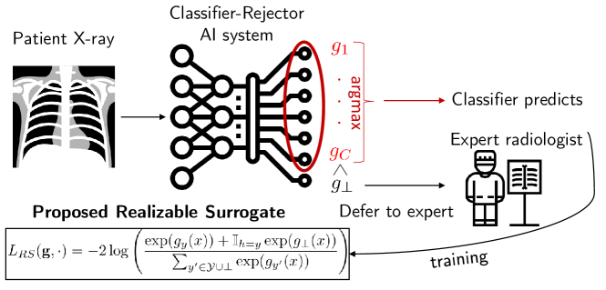
Figure 1: The learning to defer setting with the RealizableSurrogate illustrated in the application of making predictions for chest X-rays.

As a motivating example, suppose we want to build an AI system to predict the presence of pneumonia from a patient’s chest X-ray, jointly with a human radiologist. The goal of this work is to jointly learn a classifier that can predict pneumonia and a rejector, which decides on each data point whether the classifier or the human should predict illustrated in Figure 1. By learning the classifier jointly with the rejector, the aim is for the classifier to complement the radiologist so that the Human-AI team performance is higher. We refer to the error rate of the Human-AI team as the system error.

Failure of Prior Approaches. Existing literature has focused on surrogate loss functions for deferral (Madras et al., 2018; Mozannar and Sontag, 2020; Verma and Nalisnick, 2022) and confidence-based approaches (Raghu et al., 2019; Okati et al., 2021). We give a simple synthetic setting where all of these approaches fail to find a classifier/rejector pair with a low system error. In this setting, there exists a halfspace classifier and halfspace rejector that have zero system error (illustrated in Figure 2), but our experiments in Section 7.2 demonstrate that all prior approaches fail to find a good classifier/rejector pair in this setting.

To understand possible reasons for this failure, we first study the computational complexity of learning with deferral using halfspaces for the rejector and the classifier, which we call LWD-H. The computational complexity of learning with deferral has received little attention in the literature. We prove that even in our simple setting where the data is realizable (i.e., there exists a halfspace classifier and halfspace rejector achieving zero system error), there is no polynomial-time algorithm that finds an approximately optimal pair of halfspaces unless $NP=RP$. We also extend our hardness result to approximation algorithms and when the data is not realizable by halfspaces. In contrast, training a linear classifier in the realizable linear setting can be solved in polynomial time with linear programming (Boyd and Vandenberghe, 2004).

Learning with deferral using halfspaces is also of significant practical importance. Sample efficiency is critical in learning with deferral since the training data is expensive to collect—it requires both human outputs and ground-truth labels. This motivates restricting to smaller model classes, and in particular to linear classifiers and rejectors. Linear models have the benefit of being interpretable with respect to the underlying features, which can be crucial for a human-AI deferral system. Additionally, the head tuning or linear probing paradigm, where only the final (linear) layer of a pretrained deep neural network is fine-tuned on different tasks, has become increasingly common as pretrained representations improve in quality, and it can be more robust than full fine-tuning (Kumar et al., 2022). However, as previously mentioned, existing surrogate approaches fail to find a good linear classifier and rejector even when one is guaranteed to exist. This motivates the need for an algorithm for exact minimization of the system training error.

We show that exact minimization of the system error can be formulated as a mixed integer linear program (MILP). This derivation overcomes a naive quadratic formulation of the problem. In addition to exactly minimizing the training loss, the MILP formulation allows us to easily incorporate constraints to govern the human-AI system. We show that modern commercial solvers such as Gurobi (Gurobi Optimization, LLC, 2022) are capable of solving fairly large instances of this MILP, making it a practical algorithm for the LWD-H problem. To obtain similar gains over prior approaches, but with a more scalable algorithm, we develop a new differentiable surrogate loss function $L_{RS}$, dubbed RealizableSurrogate , that can solve the LWD-H problem in the realizable setting by virtue of being realizable-consistent (Long and Servedio, 2013) for a large class of hypothesis sets that includes halfspace classifier/rejector pairs. We also show empirically that $L_{RS}$ is competitive with prior work in the non-linear setting.

In section 3, we formalize the learning with deferral problem. We then study the computational complexity of LWD-H in section 4. We introduce our MILP approach in section 5 and our new surrogate RealizableSurrogate in section 6. In section 7, we evaluate our algorithms and baselines on a wide range of benchmarks in different domains, providing the most expansive evaluation of expert deferral algorithms to date. To summarize, the contributions of this paper are the following:

• Computational Complexity of Deferral: We prove the computational hardness of PAC-learning with deferral in the linear setting.

• Mixed Integer Linear Program Formulation and RealizableSurrogate : We show how to formulate learning to defer with halfspaces as a MILP and provide a novel surrogate loss.

• Experimental Evaluation: We showcase the performance of our algorithms on a wide array of datasets and compare them to several existing baselines. We contribute a publicly available repository with implementations of existing baselines and datasets: https://github.com/clinicalml/human_ai_deferral

2 Related Work

A natural baseline for the learning to defer problem is to first learn a classifier that minimizes average misclassification error, then learn a model that predicts the probability that the human makes an error on a given example, and finally defer if the probability that the classifier makes an error is higher than that of the human. This is the approach adapted by Raghu et al. (2019). However, this does not allow the classifier to adapt to the human. Another natural approach is to model this problem as a mixture of experts: the human and the AI. This is the approach introduced by Madras et al. (2018) and adapted by Wilder et al. (2020); Pradier et al. (2021) by introducing a mixture of experts surrogates. However, this approach has been to shown to fail empirically as the loss is not easily amenable to optimization. Subsequent work (Mozannar and Sontag, 2020) introduced consistent surrogate loss functions for the learning with deferral objective, with follow-up approaches addressing limitations including better calibration (Raman and Yee, 2021; Liu et al., 2021b). Another consistent convex surrogate was proposed by Verma and Nalisnick (2022) via a one-vs-all approach. Charusaie et al. (2022) provides a family of convex surrogates for learning with deferral that generalizes prior approaches, however, our proposed surrogate does not belong to that family. Keswani et al. (2021) proposes a surrogate loss which is the sum of the loss of learning the classifier and rejector separately but that is not a consistent surrogate. De et al. (2020) proved the hardness of linear regression (not classification) where some training points are allocated to the human (not deferral but subset selection of the training data). Finally, Okati et al. (2021) proposes a method that iteratively optimizes the classifier on points where it outperforms the human on the training sample, and then learns a post-hoc rejector to predict who between the human and the AI has higher error on each point. The setting when the cost of deferral is constant has a long history in machine learning and goes by the name of rejection learning (Cortes et al., 2016; Chow, 1970; Bartlett and Wegkamp, 2008; Charoenphakdee et al., 2021) or selective classification (only predict on $x$% of data) (El-Yaniv and Wiener, 2010; Geifman and El-Yaniv, 2017; Gangrade et al., 2021; Acar et al., 2020). Our MILP formulation is inspired by work in binary linear classification that optimizes the 0-1 loss exactly (Ustun and Rudin, 2016; Nguyen and Sanner, 2013).

3 Learning with Deferral: Problem Setup

We frame the learning with deferral setting as the task of predicting a target $Y\in\mathcal{Y}=\{1,\cdots,C\}$. The classifier has access to features $X\in\mathcal{X}=\mathbb{R}^{d}$, while the human (also referred to as the expert) has access to a potentially different set of features $Z\in\mathcal{Z}$ which may include side-information beyond $X$. The human is modeled as a fixed predictor $h:\mathcal{Z}\to\mathcal{Y}$. The AI system consists of a classifier $m:\mathcal{X}\to\mathcal{Y}$ and a rejector $r:\mathcal{X}\to\{0,1\}$. When $r(x)=1$, the prediction is deferred to the human and we incur a cost if the human makes an error, plus an additional, optional penalty term: $\ell_{\textrm{HUM}}(x,y,h)=\mathbb{I}_{h\neq y}+c_{\textrm{HUM}}(x,y,h)$. When $r(x)=0$, then the classifier makes the final decision and incurs a cost with a different optional penalty term: $\ell_{\textrm{AI}}(x,y,m)=\mathbb{I}_{m\neq y}+c_{\textrm{AI}}(x,y,m)$. We can put this together into a loss function for the classifier and rejector:

$$L_{\mathrm{def}}(m,r)=\mathbb{E}_{X,Y,Z}\ [\ \ell_{\textrm{AI}}\big{(}X,Y,m(X)\big{)}\cdot\mathbb{I}_{r(X)=0}+\ell_{\textrm{HUM}}(X,Y,h(Z))\cdot\mathbb{I}_{r(X)=1}\ ].$$

In this paper we focus mostly on the cost of misclassification with no additional penalties, the deferral loss becomes a misclassification loss $L_{\mathrm{def}}^{0{-}1}(m,r)$ for the human-AI system, and the optimization problem is:

$$\operatorname*{\text{minimize}}_{m,r}L_{\mathrm{def}}^{0{-}1}(m,r):=\mathbb{P}\left[\left(\left(1-r(X)\right)m(X)+r(X)h(Z)\right)\neq Y\right].$$ (1)

Constraints. We may wish to constrain the behavior of the human-AI team when learning the classifier and rejector pair. For example, we may have a limit on the percentage of times the AI can defer to the human, due to the limited time the human may have. We express this as a coverage constraint:

$$\mathbb{P}(r(X)=1)\leq\beta.$$ (2)

Finally, it is desirable that our system does not perform differently across different demographic groups. Let $A\in\{1,\cdots,|A|\}$ denote the demographic identity of an individual. Then if we wish to equalize the error rate across demographic groups, we impose the fairness constraint $\forall a\in A$:

$$\mathbb{P}((1-r(X))m(X)+r(X)h(Z)\neq Y|A\neq a)$$

$$=\mathbb{P}((1-r(X))m(X)+r(X)h(Z)\neq Y|A=a)$$ (3)

Data. We assume access to samples $S=\{(x_{i},h(z_{i}),y_{i})\}_{i=1}^{n}$ where $h(z_{i})$ is the human’s prediction on the example, but note that we do not observe $z_{i}$, the information used by the human. We emphasize that the label $y_{i}$ and human prediction $h(z_{i})$ are different, even though $y_{i}$ could also come from humans. For example in our chest X-ray classification example, $y_{i}$ could come from a consensus of 3 or more radiologists, while $h(z_{i})$ is the prediction of a single radiologist not involved with the label. Given the dataset $S$ the system training loss is given by:

$$\hat{L}_{\mathrm{def}}^{0{-}1}(m,r):=\frac{1}{n}\sum_{i=1}^{n}\mathbb{I}_{m(x_{i})\neq y_{i}}\mathbb{I}_{r(x_{i})=0}+\mathbb{I}_{h(z_{i})\neq y_{i}}\mathbb{I}_{r(x_{i})=1}$$ (4)

In the following section, we study the computational complexity of learning with deferral using halfspaces, which reduces to studying the optimization problem (4) when $m$ and $r$ are constrained to be halfspaces.

4 Computational Complexity of Learning with Deferral

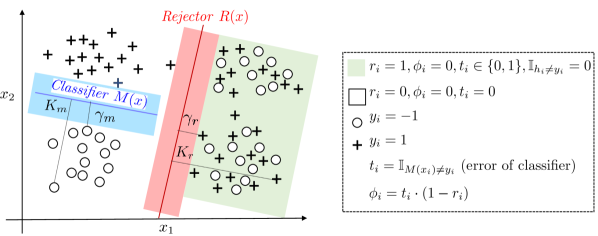
Figure 2: The realizable LWD-H setting illustrated. The task is binary classification with labels $\{o,+\}$; the human is perfect on the green-shaded region, and the data outside the green region is linearly separable. As a result, the optimal classifier and rejector obtain zero error. Assumption 2 is illustrated graphically as well as the MILP variables of equations (9)-(14).

The misclassification error of the human-AI team in equation (1) is challenging to optimize as it requires searching over a joint set of functions for the classifier and rejector, in addition to dealing with the nonconvex $0$-$1$ aspect. To study the computational complexity of minimizing the loss, we restrict our attention to a foundational setting: linear classifiers and linear rejectors in the binary label scenario.

We begin with the realizable case when there exists a halfspace classifier and rejector that can achieve zero loss:

Assumption 1 (Realizable Linear Setting).

Let $\mathcal{X}=\mathbb{R}^{d}$ and $\mathcal{Y}=\{0,1\}$. We assume that for the given expert $h$ there exists a linear classifier $m^{*}(x)=\mathbb{I}_{M^{\top}x>0}$ and a linear rejector $r^{*}(x)=\mathbb{I}_{R^{\top}x>0}$ that achieve 0 error:

$$\mathbb{E}_{(x,y,z)\sim\mathbf{P}}\ [\ \mathbb{I}_{m^{*}(x)\neq y}\mathbb{I}_{r^{*}(x)=0}+\mathbb{I}_{h(z)\neq y}\mathbb{I}_{r^{*}(x)=1}\ ]=0.$$

This setting is illustrated in Figure 2. Since the decision regions of $m$ and $r$ are halfspaces, we also use the term “halfspace” interchangeably. Note that while the classifier is assumed to be linear, the human can have a non-linear decision boundary. The analog of this assumption in the binary classification without deferral setting is to assume that there exists a halfspace that can correctly classify all the data points. In that case, we can formulate the optimization problem as a linear program to efficiently find the optimal solution (Boyd and Vandenberghe, 2004).

Hardness. In contrast to learning without deferral, we will prove that in general, it is computationally hard to learn a linear $m$ and $r$ under Assumption 1. Define the learning with deferral using halfspaces (LWD-H) problem as that of finding halfspace $m$ and halfspace $r$ such that the system error in (1) is approximately minimized.

Theorem 4.1.

Let $\epsilon>0$ be an arbitrarily small constant. Under a guarantee that there exist halfspaces $m^{*}$, $r^{*}$ with zero system loss (Assumption 1), there is no polynomial-time algorithm to find a pair of classifier-rejector halfspaces with error $1/2-\epsilon$ unless $NP=RP$.

This shows that even in the realizable setting (i.e., there exists a pair of halfspaces with zero system loss), it is hard to find a pair of halfspaces that even gets system error $1/2-\epsilon$.

Corollary 1.

There is no efficient proper PAC-learner for LWD-H unless $NP=RP$.

Proof Sketch.

First, because the true distribution of points could be supported on a finite set, the LWD-H problem boils down to approximately minimizing the training loss (4). Our proof relies on a reduction from the problem of learning an intersection of two halfspaces in the realizable setting. Let $D=\{x_{i},y_{i}\}_{i=1}^{n}$ and suppose there exists an intersection of two half-spaces $g_{1},g_{2}$ that achieve 0 error for $D$. This is an instance of learning an intersection of two halfspaces in the realizable setting, which is hard to even weakly learn (Khot and Saket, 2011). We show that this is an instance of the realizable LWD-H problem by setting $m=g_{1}$ and $r=\bar{g_{2}}$ and the human $H$ to always predict 0. Hence, an algorithm for efficiently finding a classifier/rejector pair with error $\frac{1}{2}-\epsilon$ would also find an intersection of halfspaces with error $\frac{1}{2}-\epsilon$, which is hard unless $NP=RP$. ∎

All proofs can be found in the Appendix. This hardness result holds in the realizable setting, with proper learning, and with no further assumptions on the data distribution.

Extensions. Even if the problem is not realizable and the goal is to find an approximation algorithm, this is still computationally hard as presented in the following corollary.

Corollary 2.

When the data is not realizable (i.e., Assumption 1 is violated), there is no polytime algorithm for finding a pair of halfspaces with error $\frac{1}{2}-\epsilon$ unless $NP=RP$.

Exact Solution. These hardness results motivate the need for new approaches to solving the LWD-H problem. In the next section, we derive a scheme to exactly minimize the misclassification error of the human/AI system using mixed-integer linear programming (MILP).

5 Mixed Integer Linear Program Formulation

In the previous section, we saw that in the linear setting it is computationally hard to learn an optimal classifier and rejector pair. As discussed in Section 1, we are interested in the linear setting due to the cost of labeling large datasets for learning with deferral. Linear predictors can perform similar to non-linear predictors in applications involving high-dimensional medical data (Razavian et al., 2015). Moreover, we can rely on pre-trained representations, which can allow linear predictors on top of embedded representations to attain performance comparable to non-linear predictors (Bengio et al., 2013).

A First Formulation. As a first step, we write down a mixed integer nonlinear program for the optimization of the training loss $\hat{L}_{\mathrm{def}}^{0{-}1}$ in (4) over linear classifiers and linear rejectors with binary labels. For simplicity, let $\mathcal{Y}=\{-1,+1\}$. A direct translation of (4) with halfspace classifiers and rejectors yields the following:

$$M^{*},R^{*},\cdot=\operatorname*{arg\,min}_{M,R,m_{i},r_{i}}\sum_{i=1}^{n}(1-r_{i})\mathbb{I}_{m_{i}\neq y_{i}}+r_{i}\mathbb{I}_{h_{i}\neq y_{i}}$$ (5)

$$\text{s.t.}\quad m_{i}=\textrm{sign}(M^{\top}x_{i}),\ \ r_{i}=\mathbb{I}_{R^{\top}x_{i}\geq 0}\ \forall i\in[n],$$ (6)

$$\quad M\in\mathbb{R}^{d},R\in\mathbb{R}^{d}.$$

The variables $m_{i}$ and $r_{i}$ are simply the binary outputs of the classifier and rejector. We observe that the objective involves a quadratic interaction between the classifier and rejector. Furthermore, the constraints (6) are indicator constraints that are difficult to optimize.

Making Objective Linear. We observe that since the $r_{i}$’s are binary, the term $(1-r_{i})\mathbb{I}_{m_{i}\neq y_{i}}$ can be equivalently rewritten as $\max(0,\mathbb{I}_{m_{i}\neq y_{i}}-r_{i})$. This is a crucial simplification that avoids having a mixed integer quadratic program. Below we use this to create a binary variable $t_{i}=\mathbb{I}_{m_{i}\neq y_{i}}$ representing the error of the classifier and a second continuous variable $\phi_{i}$ that upper bounds $\max(0,t_{i}-r_{i})$ and represents the classifier error after accounting for deferral.

Making Constraints Linear. Constraints (6) make sure that the binary variables $r_{i}$ and $m_{i}$ are the predictions of half-spaces $R$ and $M$ respectively. As mentioned above, we will formulate the problem using the classifier error variables $t_{i}$ instead of the classifier predictions $m_{i}$. To reformulate constraints (6) in a linear fashion, we have to make assumptions on the optimal $M$ and $R$:

Assumption 2 (Margin).

The optimal solution $(M,R)$ that minimizes the training loss (4) has margin and is bounded, meaning that $(M,R)$ satisfy the following for all $i\in[n]$ in the training set and some $\gamma_{m},\gamma_{r},K_{m},$ $K_{r}>0$:

A similar assumption is made in (Ustun and Rudin, 2016). The upper bounds in (7) are often naturally satisfied as we usually deal with bounded feature sets $\mathcal{X}$ such that we can normalize $x_{i}$ to have unit norm, and the norms of $M$ and $R$ are constrained for regularization.

Mixed Integer Linear Program. With the above ingredients and taking inspiration from the big-M approach of Ustun and Rudin (2016), we can write down the resulting mixed integer linear program (MILP):

$$M^{*},R^{*},\dots=$$

$$\operatorname*{arg\,min}_{M,R,\{r_{i}\},\{t_{i}\},\{\phi_{i}\}}\sum_{i}\phi_{i}+r_{i}\mathbb{I}_{h_{i}\neq y_{i}},\ s.t.$$ (8)

$$\phi_{i}\geq t_{i}-r_{i},\qquad\phi_{i}\geq 0\quad\forall i\in[n]$$ (9)

$$K_{m}t_{i}\geq\gamma_{m}-y_{i}M^{\top}x_{i}\quad\forall i\in[n]$$ (10)

$$R^{\top}x_{i}\leq K_{r}r_{i}+\gamma_{r}(r_{i}-1),$$ (11)

$$R^{\top}x_{i}\geq K_{r}(r_{i}-1)+\gamma_{r}r_{i}\quad\forall i\in[n]$$ (12)

$$r_{i}\in\{0,1\},t_{i}\in\{0,1\},$$ (13)

$$\phi_{i}\in\mathbb{R}^{+}\quad\forall i\in[n],\ M,R\in\mathbb{R}^{d}$$ (14)

Please see Figure 2 for a graphical illustration of the variables. We show that constraints (12) function as intended; the rest of the constraints are verified in the Appendix. When $r_{i}=0$, then we have the constraints $R^{\top}x_{i}\leq-\gamma_{r}$ and $R^{\top}x_{i}\geq-K_{r}$: this correctly forces the rejector to be negative. When $r_{i}=1$, we have $R^{\top}x_{i}\geq\gamma_{r}$ and $R^{\top}x_{i}\leq K_{r}$: which means the rejector is positive. Note that we do not need to know the margin $\gamma_{r}$ exactly, only a lower bound $\gamma$, $0<\gamma\leq\gamma_{r}$; the formulation is still correct with $\gamma$ in place of $\gamma_{r}$. However, we cannot set $\gamma=0$ as then the trivial solution $R=0$ is feasible and the constraint is void. The same statements apply to $\gamma_{m}$. This MILP has $2n$ binary variables, $n+2d$ continuous variables and $4n$ constraints. Finally, note that the MILP minimizes the 0-1 error even when Assumption 1 is violated.

Regularization and Extension to Multiclass. We can add $l_{1}$ regularization to our model by adding the $l_{1}$ norm of both $M$ and $R$ to the objective. This is done by defining two sets of variables constrained to be the $l_{1}$ norm of the classifier and rejector and adding their values to the objective in (9). Adding regularization can help prevent the MILP solution from overfitting to the training data. The above MILP only applies to binary labels but can be generalized to the multi-class setting where $\mathcal{Y}=\{1,\cdots,C\}$ (see Appendix).

Generalization Bound. Under Assumption 2 and non-realizability, assume $\lVert x_{i}\rVert_{1}\leq 1$ and constrain the search of the MILP to $M$ and $R$ with infinity norms of at most $K_{m}$ and $K_{r}$ respectively. We can relate the performance of MILP solution on the training set to the population 0-1 error.

Proposition 1.

For any expert $h$ and data distribution $\mathbf{P}$ over $\mathcal{X}\times\mathcal{Y}$ that satisfies Assumption 2, let $0<\delta<\frac{1}{2}$. Then with probability at least $1-\delta$, the following holds for the empirical minimizers $(\hat{m}^{*},\hat{r}^{*})$ obtained by the MILP:

$$L_{0{-}1}(\hat{m}^{*},\hat{r}^{*})\leq\hat{L}_{\mathrm{def}}^{0{-}1}(\hat{m}^{*},\hat{r}^{*})$$

$$+\frac{(K_{m}+K_{r})d\sqrt{2\log d}+10\sqrt{\log(2/\delta)}}{\sqrt{n\mathbb{P}(h(Z)\neq Y)}}.$$

This bound improves on surrogate optimization since the MILP will achieve a lower training error, $\hat{L}_{\mathrm{def}}^{0{-}1}(\hat{m}^{*},\hat{r}^{*})$, than the surrogate, which optimizes a different objective.

Adding Constraints. A major advantage of the MILP formulation is that it allows us to provably integrate any linear constraints on the variables with ease. For example, the constraints mentioned in Section 3 can be added to the MILP as follows in a single constraint:

• Coverage: $\sum_{i}r_{i}/n\leq\beta$

• Fairness: $\sum_{i:A=1}\bigl{(}\phi_{i}+r_{i}\mathbb{I}_{h_{i}\neq y_{i}}\bigr{)}/\lvert\{i:A=1\}\rvert=\sum_{i:A=0}\bigl{(}\phi_{i}+r_{i}\mathbb{I}_{h_{i}\neq y_{i}}\bigr{)}/\lvert\{i:A=0\}\rvert$.

So far, we have provided an exact solution to the linear learning to defer problem. However, the MILP requires significant computational time to find an exact solution for large datasets. Moreover, we might need a non-linear classifier or rejector to achieve good error. The remaining questions are (i) how to efficiently find a good pair of halfspaces for large datasets and (ii) how to generalize to non-linear predictors. In the following section, we give a novel surrogate loss function that is optimal in the realizable LWD-H setting, performs well with non-linear predictors, and can be efficiently minimized (to a local optimum).

6 Realizable Consistent Surrogate

6.1 Consistency vs Realizable Consistency

Most machine learning practice is based on optimizing surrogate loss functions of the true loss that one cares about. The surrogate loss functions are chosen so that optimizing them also optimizes the true loss functions, and also chosen to be differentiable so that they are readily optimized. This first property is captured by the notion of consistency, which was the main focus of much of the prior work on expert deferral: (Mozannar and Sontag, 2020; Verma and Nalisnick, 2022; Charusaie et al., 2022). We start by giving a formal definition of the consistency of a surrogate loss function:

Definition 1 (Consistency).

A surrogate loss function $\tilde{L}(m,r)$ is a consistent loss function for another loss $L_{\mathrm{def}}^{0{-}1}(m,r)$ if optimizing the surrogate over all measurable functions is equivalent to minimizing the original loss.

For example, the surrogates $L_{CE}$ and $\Psi_{OvA}$ both satisfy consistency for $L_{\mathrm{def}}^{0{-}1}(m,r)$ (Mozannar and Sontag, 2020; Verma and Nalisnick, 2022). It is crucial to note that consistency only applies when optimizing over all measurable functions. Conversely, in LWD-H, and in the setting of Figure 2, when we optimize with linear functions, consistency does not provide any guarantees, which explains why these methods can fail in that setting.

Since we normally optimize over a restricted model class, we want our guarantee for the surrogate to also hold for optimization under a certain model class. The notion of realizable $\mathcal{H}$-consistency is such a guarantee that has proven fruitful for classification (Long and Servedio, 2013; Zhang and Agarwal, 2020) and was extended by Mozannar and Sontag (2020) for learning with deferral. We recall the notion when extended for learning with deferral:

Definition 2 (realizable $(\mathcal{M},\mathcal{R})$-consistency).

A surrogate loss function $\tilde{L}(m,r)$ is a realizable $(\mathcal{M},\mathcal{R})$-consistent loss function for the loss $L_{\mathrm{def}}^{0{-}1}(m,r)$ if there exists a zero error solution $m^{*},r^{*}\in\mathcal{M}\times\mathcal{R}$ with $L_{\mathrm{def}}^{0{-}1}(m^{*},r^{*})=0$. Then optimizing the surrogate returns such zero error solution:

$$\widetilde{m},\widetilde{r}\in\operatorname*{arg\,inf}_{m,r\in\mathcal{M}\times\mathcal{R}}\tilde{L}(m,r)\implies L_{\mathrm{def}}^{0{-}1}(\widetilde{m},\widetilde{r})=0$$

Realizable $(\mathcal{M},\mathcal{R})$-consistency guarantees that when our data comes from some ground-truth $m^{*},r^{*}\in\mathcal{M}\times\mathcal{R}$, then minimizing the (population) surrogate loss will find an optimal $(m,r)$ pair. We propose a novel, differentiable, and $(\mathcal{M},\mathcal{R})$-consistent surrogate for learning with deferral when $\mathcal{M}$ and $\mathcal{R}$ are closed under scaling. A class $\mathcal{G}$ of scoring functions from $\mathcal{X}$ to $\mathbb{R}^{C}$ is closed under scaling if $\bm{g}\in\mathcal{G}\implies\alpha\bm{g}\in\mathcal{G}$ for any $\alpha\in\mathbb{R}$. For example, we can let $\mathcal{G}$ be the class of linear scoring functions $\bm{g}(x)=G^{\top}x$ and $G\in\mathbb{R}^{d\times C}$. Our results hold for arbitrary $\mathcal{G}$ that are closed under scaling, e.g., ReLU feedforward neural networks (FNN). We parameterize the $(m,r)$ pair with $|\mathcal{Y}|+1$ dimensional scoring function $\bm{g}:(g_{1},\ldots,g_{|\mathcal{Y}|},g_{\bot})$. We define $m(x)=\arg\max_{y\in\mathcal{Y}}g_{y}(x)$ and $r(x)=\mathbb{I}_{\max_{y\in\mathcal{Y}}g_{y}(x)\leq g_{\bot}(x)}$. The joint classifier-rejector model class $(\mathcal{M},\mathcal{R})$ is thus defined by $\mathcal{G}$, and we say $(\mathcal{M},\mathcal{R})$ is closed under scaling whenever $\mathcal{G}$ is closed under scaling. The proposed new surrogate loss $L_{RS}$, dubbed RealizableSurrogate, is defined at each point $(x,y,h)$ as:

$$L_{RS}(\mathbf{g},\cdot)=-2\log\left(\frac{\exp(g_{y}(x))+\mathbb{I}_{h=y}\exp(g_{\bot}(x))}{\sum_{y^{\prime}\in\mathcal{Y}\cup\bot}\exp(g_{y^{\prime}}(x))}\right)$$ (15)

6.2 Derivation of Surrogate

We now derive our proposed surrogate RealizableSurrogate with a principled approach. In this paper, our primary goal is to predict a target $Y$ given a set of covariates $X$ while having the ability to query a human $H$ to predict. Our overall predictor is denoted as $\hat{Y}$, a function of both $H$ and $X$, our goal is learning a predictor that maximizes the agreement between $\hat{Y}$ and $Y$:

$$\mathbb{E}[\mathbb{I}_{\hat{Y}(X,H)=Y}]=\mathbb{E}_{X}\left[\mathbb{P}(\hat{Y}(x,H)=Y|X=x)\right]$$

It will be easier to maximize the logarithm of the probability and thus using Jensen’s inequality we obtain an upper bound :

$$\log\left(\mathbb{E}_{X}\left[\mathbb{P}(\hat{Y}(x,H)=Y|X=x)\right]\right)\leq\mathbb{E}_{X}\left[\log\left(\mathbb{P}(\hat{Y}(x,H)=Y|X=x)\right)\right]$$

We now decompose our predictor into a classifier-rejector pair $(m,r)$ where the rejector decides if the classifier or the human should predict. This transforms our objective to:

$$L=\mathbb{E}_{X}\left[\log\left(\mathbb{P}(\hat{Y}=Y|X=x)\right)\right]=$$

$$\mathbb{E}_{X}\left[\log\left(\mathbb{P}(\hat{Y}=Y|X=x,r(x)=0)\mathbb{P}(r(x)=0|X=x)+\mathbb{P}(\hat{Y}=Y|X,r(x)=1)\mathbb{P}(r(x)=1|X=x)\right)\right]$$

$$=\mathbb{E}_{X}\left[\log\left(\mathbb{P}(m(x)=Y|X=x)\mathbb{P}(r(x)=0|X=x)+\mathbb{P}(H=Y|X=x)\mathbb{P}(r(x)=1|X=x)\right)\right]$$ (16)

In Madras et al. (2018), their proposed loss splits the sum inside the log above into a sum of log-likelihoods of the classifier and expert each weighted by the probability of predicting and deferring respectively. Instead in this work, we try to optimize the above log likelihood $L$ (16) directly.

Parameterization.

We now try to understand how we can parameterize the classifier-rejector pair. We first parameterize the classifier with a set of scoring functions $g_{y}:\mathcal{X}\to\mathbb{R}$ for $y\in\mathcal{Y}$ and define the classifier as the label $y$ that attains the maximum value among the set $\{g_{y^{\prime}}\}_{y^{\prime}\in\mathcal{Y}}$. To parameterize the rejector $r$, we define a single scoring function $g_{\bot}:\mathcal{X}\to\mathbb{R}$ and defer if $g_{\bot}>\max_{y}g_{y}$ which induces a comparison between the function $g_{\bot}$ and the classifier scores. One could instead parameterize the rejector $r$ with a single function $g_{\bot}:\mathcal{X}\to\mathbb{R}$ and defer if $g_{\bot}(x)$ is positive, we find empirically that the previous parameterization has better performance .

However, with the characterization, both our classifier and rejector are deterministic. Plugging in the parameterization of $(m,r)$ into the loss in (16) would result in a loss function that is non-differentiable in the parameters $g_{y}$ and $g_{\bot}$ due to thresholding. Instead, we allow the classifier and rejector to only be probabilistic during training by defining:

$$\mathbb{P}(m(x)=Y|X=x)=\frac{\exp(g_{Y}(x))}{\sum_{y^{\prime}\in\mathcal{Y}}\exp(g_{y^{\prime}}(x))},\quad\mathbb{P}(r(x)=1|X=x)=\frac{\exp(g_{\bot}(x))}{\sum_{i\in\mathcal{Y}\cup\bot}\exp(g_{i}(x))}$$

This transforms the log liklelihood $L$ to:

$$\mathbb{E}_{X}\left[\log\left(\frac{\exp(g_{Y}(x))}{\sum_{y^{\prime}\in\mathcal{Y}}\exp(g_{y^{\prime}}(x))}\cdot\frac{\sum_{y^{\prime}\in\mathcal{Y}}\exp(g_{y^{\prime}}(x))}{\sum_{i\in\mathcal{Y}\cup\bot}\exp(g_{i}(x))}+\mathbb{P}(H=Y|X)\cdot\frac{\exp(g_{\bot}(x))}{\sum_{i\in\mathcal{Y}\cup\bot}\exp(g_{i}(x))}\right)\right]$$

$$=-\mathbb{E}_{X}\left[\log\left(\frac{\exp(g_{Y}(x))+\mathbb{P}(H=Y|X)\exp(g_{\bot}(x))}{\sum_{y^{\prime}\in\mathcal{Y}}\exp(g_{y^{\prime}}(x))}\right)\right]$$

We multiple the above likelihood by $-2$ so that we can instead minimize a loss and so that it becomes an upper bound of the $0-1$ deferral loss $L_{\mathrm{def}}^{0{-}1}(m,r)$. Given the dataset $S$, our proposed loss then becomes:

$$L_{RS}^{S}=-2\sum_{i=1}^{n}\log\left(\frac{\exp(g_{y_{i}}(x_{i}))+\mathbb{I}_{h(z_{i})=y_{i}}\exp(g_{\bot}(x))}{\sum_{y^{\prime}\in\mathcal{Y}}\exp(g_{y^{\prime}}(x))}\right)$$ (17)

6.3 Theoretical Guarantees

Notice in our proposed loss $L_{RS}$ that when the human is incorrect, i.e. $\mathbb{I}_{h=y}=0$, the loss incentivizes the classifier to be correct, similar to cross entropy loss. However, when the human is correct, the learner has the choice to either fit the target or defer: there is no penalty for choosing to do one or the other. This is what enables the classifier to complement the human and differentiates $L_{RS}$ from prior surrogates, such as $L_{CE}$ (Mozannar and Sontag, 2020), that are not realizable-consistent (see Theorem LABEL:apx:the_realiza_not in Appendix LABEL:apx:proffs_sec_realiz) and penalize the learner for not fitting the target even when deferring. This property is showcased by the fact that our surrogate is realizable $(\mathcal{M},\mathcal{R})$-consistent for model classes that are closed under scaling. Moreover, it is an upper bound of the true loss $L_{\mathrm{def}}^{0{-}1}(m,r)$. The theorem below characterizes the properties of our novel surrogate function.

Theorem 6.1.

The RealizableSurrogate $L_{RS}$ is a realizable $(\mathcal{M},\mathcal{R})$-consistent surrogate for $L_{\mathrm{def}}^{0{-}1}$ for model classes closed under scaling, and satisfies $L_{\mathrm{def}}^{0{-}1}(m,r)\leq L_{RS}(m,r)$ for all $(m,r)$.

This theorem implies that when Assumption 1 is satisfied and $\mathcal{G}$ is the class of linear scoring functions, minimizing $L_{RS}$ yields a classifier-rejector pair with zero system error. The resulting classifier is the halfspace $\mathbb{I}((G_{1}-G_{0})^{\top}x\geq 0)$ and the form of the rejector is $\mathbb{I}((G_{\bot}^{\top}x-\max(G_{1}^{\top}x,G_{0}^{\top}x))\geq 0)$, which is an intersection of halfspaces. One can obtain a halfspace rejector by minimizing instead with the parameterization of $L_{RS2}$.

The surrogate is differentiable but non-convex in $\mathbf{g}$, though it is convex in each $g_{i}$. Indeed, a jointly convex surrogate that provably works in the realizable linear setting would contradict Theorem 4.1. In practice, we observe that in the linear realizable setting, the local minima reached by gradient descent obtain zero training error despite the nonconvexity. The mixture-of-experts surrogate in Madras et al. (2018) is realizable $(\mathcal{M},\mathcal{R})$-consistent, non-convex and not classification consistent as shown by Mozannar and Sontag (2020), however, Mozannar and Sontag (2020) also showed that it leads to worse empirical results than simple baselines. We have not been able to prove or disprove that RealizableSurrogateis classification-consistent, unlike other surrogates like that of Mozannar and Sontag (2020). It remains an open problem to find both a consistent and a realizable-consistent surrogate.

6.4 Underfitting The Target

Minimizing the proposed loss leads to a classifier that attempts to complement the human. One consequence is that the classifier might have high error on points that are deferred to the human, resulting in possibly high error across a large subset of the data domain. We can explicitly encourage the classifier to fit the target on all points by adding an extra term to the loss:

$$\leavevmode\resizebox{208.13574pt}{}{$L_{RS}^{\alpha}(\mathbf{g},x,y,h)=-\alpha\log\left(\frac{\exp(g_{y}(x)+\mathbb{I}_{h=y}\exp(g_{\bot}(x))}{\sum_{y^{\prime}\in\mathcal{Y}\cup\bot}\exp(g_{y^{\prime}}(x))}\right)$}-(1-\alpha)\log\left(\frac{\exp(g_{y}(x))}{\sum_{y^{\prime}\in\mathcal{Y}}\exp(g_{y^{\prime}}(x))}\right)$$ (18)

The new loss $L_{RS}^{\alpha}$ with $\alpha\in[0,1]$ (a hyperparameter) is a convex combination of $L_{RS}$ and the cross entropy loss for the classifier (with the softmax applied only over the functions $g_{y}$ rather than including $g_{\bot}$). Empirically, this allows the points that are deferred to the human to still help provide extra training signal to the classifier, which is useful for sample-efficiency when training complex, non-linear hypotheses. Finally, due to adding the parameter $\alpha$, the loss no longer remains realizable consistent, thus we let the rejector be $r(x)=\mathbb{I}_{g_{\bot}(x)-\max_{y}g_{y}(x)\geq\tau}$ and we learn $\tau$ with a line search to maximize system accuracy on a validation set. In the next section, we evaluate our approaches with an extensive empirical benchmark.

7 Experiments

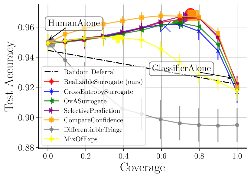
(a) CIFAR-10H

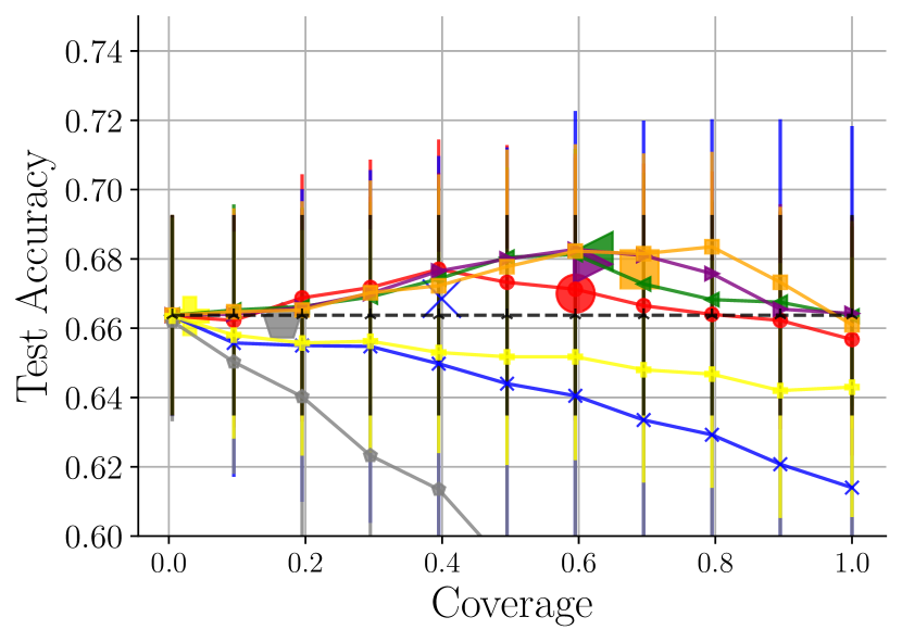
(b) COMPASS

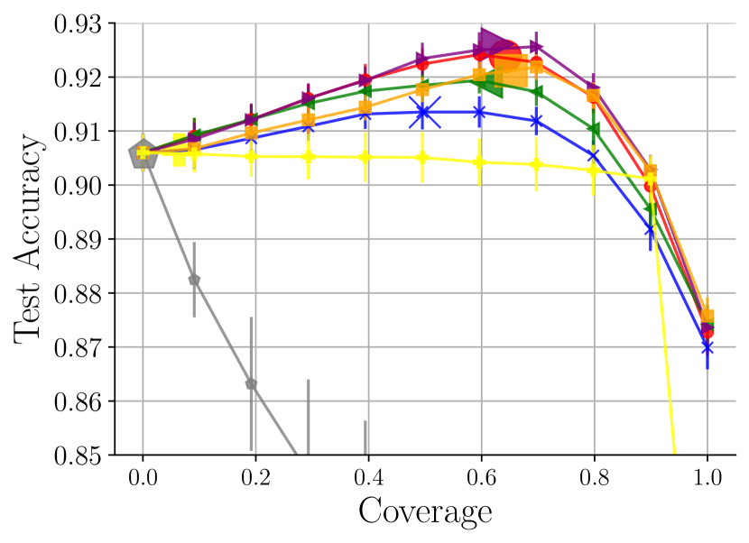
(c) HateSpeech

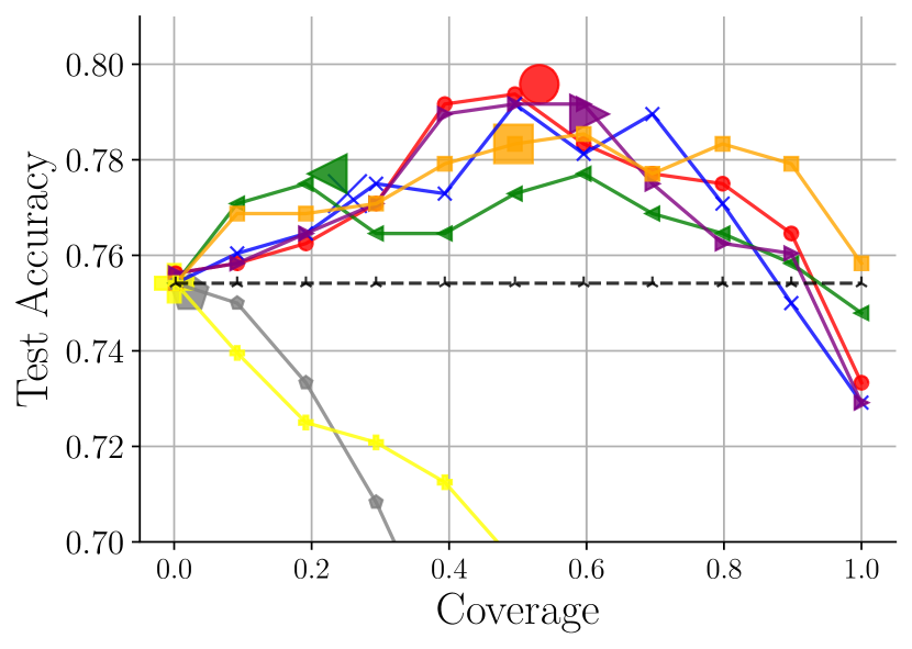
(d) ImageNet-16H

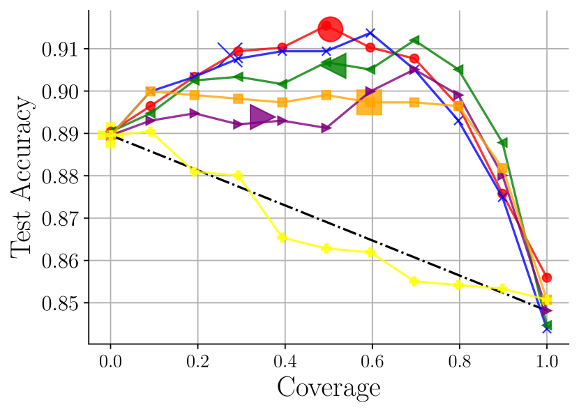
(e) Chest X-ray - Airspace Opacity

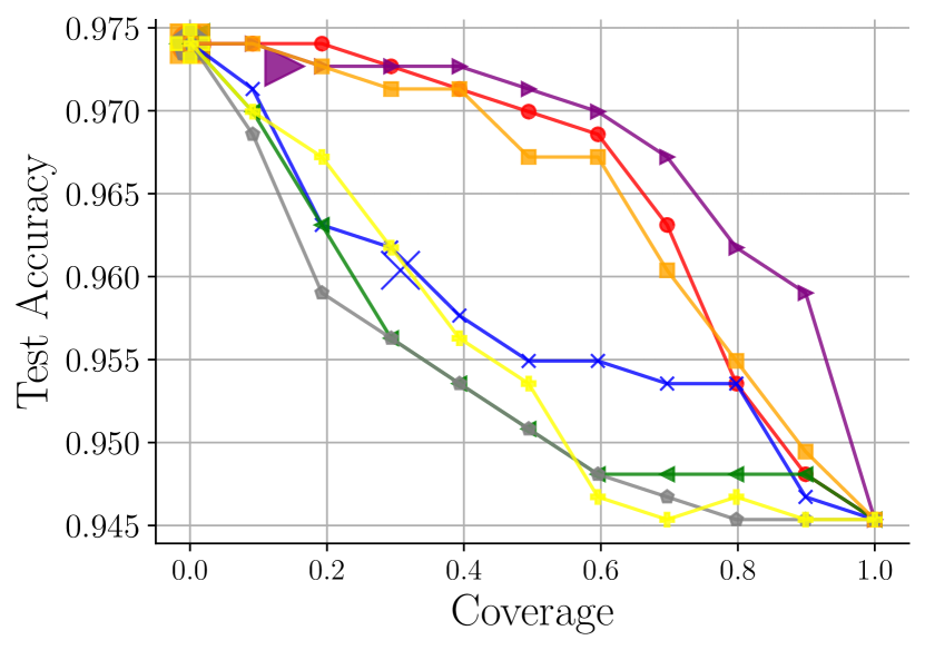
(f) Chest X-ray - Pneumothorax

Figure 3: Accuracy vs coverage (fraction of points where classifier predicts) plots across the real world datasets showcasing the behavior of our method and the baselines. On each plot, we showcase the test accuracy of each method with a large marker, with the curve representing varying the rejector threshold on the test set. To achieve different levels of coverage, we sort the rejection score for each method on the test set and vary the threshold used, for RealizableSurrogate the rejector is defined as $r(x)=\mathbb{I}_{g_{\bot}(x)-\max_{y}g_{y}(x)\geq c}$ where the optimal solution is at $c=0$ and we vary $c\in\mathbb{R}$ to obtain the curve.

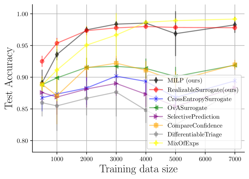
(a) Synthetic Data Sample Complexity

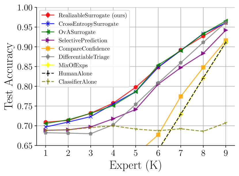
(b) CIFAR-K Semi-Synthetic

Figure 4: (a) Test performance of the different methods on synthetic data as we increase the training data size and repeat the randomization over 10 trials to get standard errors. (b) Test performance on the semi-synthetic CIFAR-K dataset vs. the number of classes $K$ for which the expert is perfect.

Table 1: Datasets used for our benchmark for learning with deferral to humans. We note the total number of samples $n$, the target set size $|\mathcal{Y}|$, the number of tasks in each dataset (a task is a set of human and target labels), the human expert where ’random annotator’ means that for each point we have multiple human annotations and we let the target be a consensus and the human label be a random sample while ’separate human annotation’ means that the human label is completely separate from the label annotations and finally the model class for both the classifier and rejector.

Dataset	$n$	$\left|\mathcal{Y}\right|$	Number of Tasks	Human	Model Class
SyntheticData (ours)	arbitrary	2	1	synthetic	linear
CIFAR-K	60k	10	10 (per expert $k$)	synthetic (perfect on k classes)	CNN
CIFAR-10H (Battleday et al., 2020)	10k	10	1	separate human annotation	pretrained WideResNet (Zagoruyko and Komodakis, 2016)
Imagenet-16H (Kerrigan et al., 2021)	1.2k	16	4 (per noise version)	separate human annotation	pretrained DenseNet121 (Huang et al., 2017), finetuning last layer only
HateSpeech (Davidson et al., 2017)	25k	3	1	random annotator	FNN on embeddings from SBERT (Reimers and Gurevych, 2019)
COMPASS (Dressel and Farid, 2018)	1k	2	1	separate human annotation	linear
NIH Chest X-ray (Wang et al., 2017; Majkowska et al., 2020)	4k	2	4 (for different conditions)	random annotator	pretrained DenseNet121 on non-human labeled data

7.1 Human-AI Deferral Benchmark

Objective. We investigate the empirical performance of our proposed approaches compared to prior baselines on a range of datasets. Specifically, we want to compare the accuracy of the human-AI team at the learned classifier-rejector pairs. We also check the accuracy of the system when we change the deferral policy by varying the threshold used for the rejector, this leads to an accuracy-coverage plot where coverage is defined as the fraction of the test points where the classifier predicts.

Datasets. In Table 1 we list the datasets used in our benchmark. We start with synthetic data described below, then semi-synthetic data with CIFAR-K (Mozannar and Sontag, 2020). We then evaluate on 5 real world datasets with three image classification domains with multiple tasks per domain, a natural language domain and a tabular domain. Each dataset is randomly split 70-10-20 for training-validation-testing respectively.

Baselines. We compare to multiple methods from the literature including: the confidence method from Raghu et al. (2019) (CompareConfidence), the surrogate $L_{CE}^{\alpha}$ from Mozannar and Sontag (2020) (CrossEntropySurrogate), the surrogate $\Psi_{\textrm{OvA}}$ from Verma and Nalisnick (2022) (OvASurrogate), Diff-Triage from Okati et al. (2021) (DifferentiableTriage), mixture of experts from Madras et al. (2018) (MixOfExps) and finally a selective prediction baseline that thresholds classifier confidence for the rejector (SelectivePrediction). For all baselines and datasets, we train using Adam and use the same learning rate and the same number of training epochs to ensure an equal footing across baselines, each run is repeated for 5 trials with different dataset splits. We track the best model in terms of system accuracy on a validation set for each training epoch and return the best-performing model. For RealizableSurrogate , we perform a hyperparameter search on the validation set over $\alpha\in[0,1]$, and do hyperparameter tuning over $L_{CE}^{\alpha}$.

7.2 Synthetic and Semi-Synthetic Data

Synthetic Data. We create a set of synthetic data distributions that are realizable by linear functions (or nearly so) to benchmark our approach. For the input $X$, we set the dimension $d$, and experiment with two data distributions. (1) Uniform distribution: we draw points $X\sim\mathrm{Unif}(0,U)^{d}$ where $U\in\mathbb{R}^{+}$; (2) Mixture-of-Gaussians: we fix some $K\in\mathbb{N}$ and generate data from $K$ equally weighted Gaussians, each with random uniform means and variances. To obtain labels $Y$ that satisfy Assumption 1, we generate two random halfspaces and denote one as the optimal classifier $m^{*}(x)$ and the other as the optimal rejector $r^{*}(x)$. We then set the labels $Y$ on the side where $r^{*}(x)=0$ to be consistent with $m^{*}(x)$ with probability $1-p_{m}$ and otherwise uniform. When $r^{*}(x)=1$, we sample the labels uniformly. Finally, we choose the human expert to have error $p_{h0}$ when $r^{*}(x)=0$ and have error $p_{h1}$ when $r^{*}(x)=1$. When $p_{m}=0,p_{h0}\in[0,1]$, and $p_{h1}=0$, this process generates datasets $D=\{x_{i},y_{i},h_{i}\}_{i=1}^{n}$ that satisfy Assumption 1.

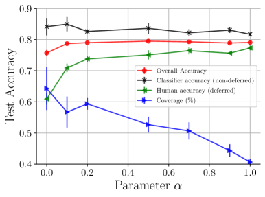
Figure 5: Sensitivity of the RealizableSurrogate to the hyperparameter $\alpha$. We vary the hyperparameter $\alpha$ in the RealizableSurrogate surrogate loss and show the different metrics including overall accuracy, accuracy when we defer, accuracy when we don’t defer, and finally coverage.

Sample Complexity. For realizable data with a feature distribution that is mixture of Gaussians ($d=30$, $p_{m}=0,p_{h0}=0.3,p_{h1}=0$), Figure 4(a) plots the test accuracy of the different methods on a held-out dataset of 5k points as we increase the training data size. We observe that MILP and RealizableSurrogate are able to get close to zero error, while all other methods fail at finding a near zero-error solution. We also experiment with non-realizable data. For example, when $p_{m}=0.1,p_{h0}=0.4,p_{h1}=0.1$ with $n=1000$, the optimal test error is $7.5\pm 1.0\%$ for the generated data: the MILP obtains $11.2$ error and RealizableSurrogate achieves $17.8\pm 1.0$ error, while the best baseline CrossEntropySurrogate achieves $21.4\pm 1.1$ error. In the Appendix, we show results on the uniform data distribution, which shows an identical pattern, and we study the run-time and performance of the MILP as we increase the error probabilities.

CIFAR-K. We use the CIFAR-10 image classification dataset (Krizhevsky et al., 2009) and employ a simple convolution neural network (CNN) with three layers. We consider the human expert models from Mozannar and Sontag (2020); Verma and Nalisnick (2022): if the image is in the first $K$ classes the expert is perfect, otherwise the expert predicts randomly. Figure 4(b) shows the test accuracy of the different methods as we vary the expert strength $K$. RealizableSurrogate outperforms the second-best method by 0.8% on average and up to 2.8% maximum showcasing that the method can perform well for non-linear predictors.

7.3 Realistic Data

Models. In Figure 3, we showcase the test accuracy of the different baselines on the real datasets in Table 1, and illustrate their behavior when we constrain our method and the baselines to achieve different levels of coverage. The test accuracy of the operating point on the different datasets is shown in Table 2. We can see that $L_{RS}^{\alpha}$ is competitive with the best baseline on each dataset/task. Moreover, we see that the human-AI team is often able to achieve performance that is higher than the human or classifier on their own. The methods often achieve peak performance at a coverage rate that is not at the extremes of [0,1], and on each of the six datasets we notice variability between the peak accuracy coverage rate indicating tat they are finding different solutions. This demonstrates that deferral using $L_{RS}^{\alpha}$ is able to achieve complementary human-AI team performance in practice. In summary, the new surrogate $L_{RS}$ performs as well as the MILP on synthetic data, and as well as all the baselines (or better) on real-world data. Note that Differentiable Triage on these datasets is underperforming as we are testing it on a setting beyond the paper as here we only have samples of expert predictions instead of probabilities from the expert.

Table 2: Test accuracy of the operating point of the different methods on the datasets tested on. The baselines are $L_{CE}$ (Mozannar and Sontag, 2020), $\Psi_{\textrm{OvA}}$ (Verma and Nalisnick, 2022), Selective Prediction (SP), Compare Confidence (CP) (Raghu et al., 2019), DIFT (Okati et al., 2021) and MoE (Madras et al., 2018).

Dataset	$L_{RS}^{\alpha}$ (ours)	$L_{CE}$	$\Psi_{\textrm{OvA}}$	SP	CC	DIFT	MoE
Synthetic Realizable	0.979	0.891	0.918	0.882	0.918	0.870	0.992
Synthetic Non-Realizable	0.879	0.828	0.839	0.797	0.836	0.770	0.774
Cifar-K (K=5)	0.795	0.785	0.786	0.747	0.621	0.749	0.550
Compass	0.670	0.668	0.682	0.678	0.677	0.662	0.663
Cifar-10H	0.969	0.960	0.963	0.966	0.968	0.949	0.953
Hate Speech	0.924	0.913	0.919	0.926	0.921	0.906	0.907
ImageNet16H (noise 80)	0.912	0.908	0.909	0.910	0.908	0.898	0.904
ImageNet16H (noise 95)	0.865	0.872	0.872	0.875	0.868	0.856	0.861
ImageNet16H (noise 110)	0.802	0.791	0.791	0.809	0.792	0.756	0.761
ImageNet16H (noise 125)	0.755	0.707	0.732	0.756	0.743	0.655	0.604
Pneumothorax	0.976	0.963	0.978	0.972	0.978	0.978	0.978
Airspace Opacity	0.913	0.908	0.906	0.899	0.905	0.894	0.894

Hyperparameter $\alpha$.

We show how the behavior of the classifier and rejector system changes when we modify the hyperparameter $\alpha\in[0,1]$ in Figure 5. When $\alpha$ is small, the behavior of the surrogate is the same as selective prediction which is why we see the lowest accuracy of the human when we defer. As $\alpha$ increases to $1$, we can see that the system better adapts to the human.

Recommendations: Which Method to Use?

Given our experimental results, the question to ask is which method should be used for a given dataset and model class. The simple and natural baseline of CompareConfidence should be the first tool one applies to their setting, it often achieves good performance, outperforming the naive baseline SelectivePrediction. However, CompareConfidence does not allow the classifier to adapt to the humans strengths and weaknesses. The surrogates CrossEntropySurrogate and OvASurrogate when applied with expressive model classes such as deep networks can find complementary classifiers. The surrogates offer other advantages, notably, CrossEntropySurrogate has been shown to have better sample complexity over the CompareConfidence baseline and can incorporate arbitrary costs of deferral and prediction (Mozannar and Sontag, 2020). However, as our synthetic experiments have shown, there is a limit of the CrossEntropySurrogate and OvASurrogate surrogats to how much they can complement the human and defer accordingly. This is where our proposed methods MILPDefer and RealizableSurrogate come in. We recommend using the MILP in settings with limited data where linear models are suitable as it can achieve optimal performance, however, one must carefully tune regularization parameters to not overfit. If the data is realizable, then the RealizableSurrogate is also optimal and is much easier to optimize, one can apply the surrogate without knowing beforehand if the data is realizable. RealizableSurrogate works well with linear and non-linear model classes, and performs the best under model resource constraints, we recommend using it broadly when optimizing accuracy.

8 Conclusion

We have shown that properly learning halfspaces with deferral (LWD-H) is computationally hard and that existing approaches in the literature fail in this setting. Understanding the computational limits of learning to defer led to the design of a new exact algorithm (the MILP) and a new surrogate (RealizableSurrogate) that both obtain better empirical performance than existing surrogate approaches. Studying $(\mathcal{M},\mathcal{R})$-consistency in the non-realizable setting, obtaining conditions under which nonconvex surrogates like $L_{RS}$ can be provably and efficiently minimized, and considering online versions of learning to defer are interesting directions for future work. As human-AI teams are deployed in real-world decision-making scenarios, better and safer methods for training these systems are of critical interest. Giving the AI the power to allow the human to predict or not requires very careful optimization of the rejector so that we have favorable outcomes, this motivates the need for exact algorithms with guarantees.

Appendix A Practitioner’s guide to our approach

A.1 MILP

We implement the MILP (9)-(14) in the binary setting using the Gurobi Optimizer Gurobi Optimization, LLC (2022) in Python.

class MILPDefer: def __init__(self, n_classes, time_limit=-1, add_regularization=False, lambda_reg=1, verbose=False): self.n_classes = n_classes self.time_limit = time_limit self.verbose = verbose self.add_regularization = add_regularization self.lambda_reg = lambda_reg

def fit(self, dataloader_train, dataloader_val, dataloader_test): self.fit_binary(dataloader_train, dataloader_val, dataloader_test)

def fit_binary(self, dataloader_train, dataloader_val, dataloader_test): data_x = dataloader_train.dataset.tensors[0] data_y = dataloader_train.dataset.tensors[1] human_predictions = dataloader_train.dataset.tensors[2]

C = 1 gamma = 0.00001 Mi = C + gamma Ki = C + gamma max_data = len(data_x) hum_preds = 2*np.array(human_predictions) - 1 # add extra dimension to x data_x_original = torch.clone(data_x) norm_scale = max(torch.norm(data_x_original, p=1, dim=1)) last_time = time.time() # normalize data_x and then add dimension data_x = torch.cat((torch.ones((len(data_x)), 1), data_x/norm_scale), dim=1).numpy() data_y = 2*data_y - 1 # covert to 1, -1 max_data = max_data # len(data_x) dimension = data_x.shape[1]

model = gp.Model("milp_deferral") model.Params.IntFeasTol = 1e-9 model.Params.MIPFocus = 0 if self.time_limit != -1: model.Params.TimeLimit = self.time_limit

H = model.addVars(dimension, lb=[-C] * dimension, ub=[C]*dimension, name="H") Hnorm = model.addVars( dimension, lb=[0]*dimension, ub=[C]*dimension, name="Hnorm") Rnorm = model.addVars( dimension, lb=[0]*dimension, ub=[C]*dimension, name="Rnorm") R = model.addVars(dimension, lb=[-C] * dimension, ub=[C]*dimension, name="R") phii = model.addVars(max_data, vtype=gp.GRB.CONTINUOUS, lb=0) psii = model.addVars(max_data, vtype=gp.GRB.BINARY) ri = model.addVars(max_data, vtype=gp.GRB.BINARY)

equal = np.array(data_y) == hum_preds * 1.0 human_err = 1-equal

if self.add_regularization: model.setObjective(gp.quicksum([phii[i] + ri[i]*human_err[i] for i in range(max_data)])/max_data + self.lambda_reg * gp.quicksum( [Hnorm[j] for j in range(dimension)]) + self.lambda_reg * gp.quicksum([Rnorm[j] for j in range(dimension)])) else: model.setObjective(gp.quicksum( [phii[i] + ri[i]*human_err[i] for i in range(max_data)])/max_data) for i in range(max_data): model.addConstr(phii[i] >= psii[i] - ri[i], name="phii" + str(i)) model.addConstr(Mi*psii[i] >= gamma - data_y[i]*gp.quicksum( H[j] * data_x[i][j] for j in range(dimension)), name="psii" + str(i)) model.addConstr(gp.quicksum([R[j]*data_x[i][j] for j in range(dimension)]) >= Ki*( ri[i]-1) + gamma*ri[i], name="Riub" + str(i)) model.addConstr(gp.quicksum([R[j]*data_x[i][j] for j in range( dimension)]) <= Ki*ri[i] + gamma*(ri[i]-1), name="Rilb" + str(i)) model.update() if self.add_regularization: for j in range(dimension): model.addConstr(Hnorm[j] >= H[j], name="Hnorm1" + str(j)) model.addConstr(Hnorm[j] >= -H[j], name="Hnorm2" + str(j)) model.addConstr(Rnorm[j] >= R[j], name="Rnorm1" + str(j)) model.addConstr(Rnorm[j] >= -R[j], name="Rnorm2" + str(j))

model.ModelSense = 1 # minimize model._time = time.time() model._time0 = time.time() model._cur_obj = float(’inf’) # model.write(’model.lp’) if self.verbose: model.optimize() else: model.optimize() # check if halspace solution has 0 error error_v = 0 rejs = 0 for i in range(max_data): rej_raw = np.sum([R[j].X * data_x[i][j] for j in range(dimension)]) pred_raw = np.sum([H[j].X * data_x[i][j] for j in range(dimension)]) if rej_raw > 0: rejs += 1 error_v += (data

References

- Acar et al. (2020) D. A. E. Acar, A. Gangrade, and V. Saligrama. Budget learning via bracketing. In International Conference on Artificial Intelligence and Statistics, pages 4109–4119. PMLR, 2020.
- Bartlett and Wegkamp (2008) P. L. Bartlett and M. H. Wegkamp. Classification with a reject option using a hinge loss. Journal of Machine Learning Research, 9(Aug):1823–1840, 2008.
- Bartlett et al. (2006) P. L. Bartlett, M. I. Jordan, and J. D. McAuliffe. Convexity, classification, and risk bounds. Journal of the American Statistical Association, 101(473):138–156, 2006.
- Battleday et al. (2020) R. M. Battleday, J. C. Peterson, and T. L. Griffiths. Capturing human categorization of natural images by combining deep networks and cognitive models. Nature communications, 11(1):1–14, 2020.
- Beede et al. (2020) E. Beede, E. Baylor, F. Hersch, A. Iurchenko, L. Wilcox, P. Ruamviboonsuk, and L. M. Vardoulakis. A human-centered evaluation of a deep learning system deployed in clinics for the detection of diabetic retinopathy. In Proceedings of the 2020 CHI Conference on Human Factors in Computing Systems, pages 1–12, 2020.
- Bengio et al. (2013) Y. Bengio, A. Courville, and P. Vincent. Representation learning: A review and new perspectives. IEEE transactions on pattern analysis and machine intelligence, 35(8):1798–1828, 2013.
- Blum and Rivest (1988) A. Blum and R. Rivest. Training a 3-node neural network is np-complete. Advances in neural information processing systems, 1, 1988.
- Boyd and Vandenberghe (2004) S. Boyd and L. Vandenberghe. Convex optimization. Cambridge university press, 2004.
- Charoenphakdee et al. (2021) N. Charoenphakdee, Z. Cui, Y. Zhang, and M. Sugiyama. Classification with rejection based on cost-sensitive classification. In International Conference on Machine Learning, pages 1507–1517. PMLR, 2021.
- Charusaie et al. (2022) M.-A. Charusaie, H. Mozannar, D. Sontag, and S. Samadi. Sample efficient learning of predictors that complement humans. In International Conference on Machine Learning, pages 2972–3005. PMLR, 2022.
- Chow (1970) C. Chow. On optimum recognition error and reject tradeoff. IEEE Transactions on information theory, 16(1):41–46, 1970.
- Cortes et al. (2016) C. Cortes, G. DeSalvo, and M. Mohri. Learning with rejection. In International Conference on Algorithmic Learning Theory, pages 67–82. Springer, 2016.
- Davidson et al. (2017) T. Davidson, D. Warmsley, M. Macy, and I. Weber. Automated hate speech detection and the problem of offensive language. In Eleventh international aaai conference on web and social media, 2017.
- De et al. (2020) A. De, P. Koley, N. Ganguly, and M. Gomez-Rodriguez. Regression under human assistance. In Proceedings of the AAAI Conference on Artificial Intelligence, volume 34, pages 2611–2620, 2020.
- Dressel and Farid (2018) J. Dressel and H. Farid. The accuracy, fairness, and limits of predicting recidivism. Science advances, 4(1):eaao5580, 2018.
- El-Yaniv and Wiener (2010) R. El-Yaniv and Y. Wiener. On the foundations of noise-free selective classification. Journal of Machine Learning Research, 11(May):1605–1641, 2010.
- Gangrade et al. (2021) A. Gangrade, A. Kag, and V. Saligrama. Selective classification via one-sided prediction. In International Conference on Artificial Intelligence and Statistics, pages 2179–2187. PMLR, 2021.
- Geifman and El-Yaniv (2017) Y. Geifman and R. El-Yaniv. Selective classification for deep neural networks. In Advances in neural information processing systems, pages 4878–4887, 2017.
- Gurobi Optimization, LLC (2022) Gurobi Optimization, LLC. Gurobi Optimizer Reference Manual, 2022. URL https://www.gurobi.com.
- Guruswami and Raghavendra (2009) V. Guruswami and P. Raghavendra. Hardness of learning halfspaces with noise. SIAM Journal on Computing, 39(2):742–765, 2009.
- Huang et al. (2017) G. Huang, Z. Liu, L. Van Der Maaten, and K. Q. Weinberger. Densely connected convolutional networks. In Proceedings of the IEEE conference on computer vision and pattern recognition, pages 4700–4708, 2017.
- Jacobs et al. (2021) M. Jacobs, M. F. Pradier, T. H. McCoy, R. H. Perlis, F. Doshi-Velez, and K. Z. Gajos. How machine-learning recommendations influence clinician treatment selections: the example of antidepressant selection. Translational psychiatry, 11(1):1–9, 2021.
- Kakade and Tewari (2008) S. Kakade and A. Tewari. Rademacher composition and linear prediction. https://home.ttic.edu/~tewari/lectures/lecture17.pdf, February 2008.
- Kerrigan et al. (2021) G. Kerrigan, P. Smyth, and M. Steyvers. Combining human predictions with model probabilities via confusion matrices and calibration. Advances in Neural Information Processing Systems, 34, 2021.
- Keswani et al. (2021) V. Keswani, M. Lease, and K. Kenthapadi. Towards unbiased and accurate deferral to multiple experts. arXiv preprint arXiv:2102.13004, 2021.
- Khot and Saket (2011) S. Khot and R. Saket. On the hardness of learning intersections of two halfspaces. Journal of Computer and System Sciences, 77(1):129–141, 2011.
- Kingma and Ba (2014) D. P. Kingma and J. Ba. Adam: A method for stochastic optimization. arXiv preprint arXiv:1412.6980, 2014.
- Krizhevsky et al. (2009) A. Krizhevsky, G. Hinton, et al. Learning multiple layers of features from tiny images. Citeseer, 2009.
- Kumar et al. (2022) A. Kumar, A. Raghunathan, R. M. Jones, T. Ma, and P. Liang. Fine-tuning can distort pretrained features and underperform out-of-distribution. In International Conference on Learning Representations, 2022.
- Lin (2002) Y. Lin. Support vector machines and the bayes rule in classification. Data Mining and Knowledge Discovery, 6(3):259–275, 2002.
- Liu et al. (2021a) H. Liu, V. Lai, and C. Tan. Understanding the effect of out-of-distribution examples and interactive explanations on human-ai decision making. Proceedings of the ACM on Human-Computer Interaction, 5(CSCW2):1–45, 2021a.
- Liu et al. (2021b) J. Liu, B. Gallego, and S. Barbieri. Incorporating uncertainty in learning to defer algorithms for safe computer-aided diagnosis. arXiv preprint arXiv:2108.07392, 2021b.
- Long and Servedio (2013) P. Long and R. Servedio. Consistency versus realizable h-consistency for multiclass classification. In International Conference on Machine Learning, pages 801–809. PMLR, 2013.
- Loshchilov and Hutter (2017) I. Loshchilov and F. Hutter. Decoupled weight decay regularization. arXiv preprint arXiv:1711.05101, 2017.
- Madras et al. (2018) D. Madras, T. Pitassi, and R. Zemel. Predict responsibly: Improving fairness and accuracy by learning to defer. In Advances in Neural Information Processing Systems, pages 6150–6160, 2018.
- Majkowska et al. (2020) A. Majkowska, S. Mittal, D. F. Steiner, J. J. Reicher, S. M. McKinney, G. E. Duggan, K. Eswaran, P.-H. Cameron Chen, Y. Liu, S. R. Kalidindi, et al. Chest radiograph interpretation with deep learning models: assessment with radiologist-adjudicated reference standards and population-adjusted evaluation. Radiology, 294(2):421–431, 2020.
- Mozannar and Sontag (2020) H. Mozannar and D. Sontag. Consistent estimators for learning to defer to an expert. In International Conference on Machine Learning, pages 7076–7087. PMLR, 2020.
- Mozannar et al. (2022) H. Mozannar, A. Satyanarayan, and D. Sontag. Teaching humans when to defer to a classifier via exemplars. In Proceedings of the Thirty-Sixth AAAI Conference on Artificial Intelligence (AAAI), 2022.
- Nguyen and Sanner (2013) T. Nguyen and S. Sanner. Algorithms for direct 0–1 loss optimization in binary classification. In International Conference on Machine Learning, pages 1085–1093. PMLR, 2013.
- Okati et al. (2021) N. Okati, A. De, and M. Gomez-Rodriguez. Differentiable learning under triage. arXiv preprint arXiv:2103.08902, 2021.
- Pradier et al. (2021) M. F. Pradier, J. Zazo, S. Parbhoo, R. H. Perlis, M. Zazzi, and F. Doshi-Velez. Preferential mixture-of-experts: Interpretable models that rely on human expertise as much as possible. arXiv preprint arXiv:2101.05360, 2021.
- Raghu et al. (2019) M. Raghu, K. Blumer, G. Corrado, J. Kleinberg, Z. Obermeyer, and S. Mullainathan. The algorithmic automation problem: Prediction, triage, and human effort. arXiv preprint arXiv:1903.12220, 2019.
- Raman and Yee (2021) N. Raman and M. Yee. Improving learning-to-defer algorithms through fine-tuning. arXiv preprint arXiv:2112.10768, 2021.
- Razavian et al. (2015) N. Razavian, S. Blecker, A. M. Schmidt, A. Smith-McLallen, S. Nigam, and D. Sontag. Population-level prediction of type 2 diabetes from claims data and analysis of risk factors. Big Data, 3(4):277–287, 2015.
- Reimers and Gurevych (2019) N. Reimers and I. Gurevych. Sentence-bert: Sentence embeddings using siamese bert-networks. arXiv preprint arXiv:1908.10084, 2019.
- Ustun and Rudin (2016) B. Ustun and C. Rudin. Supersparse linear integer models for optimized medical scoring systems. Machine Learning, 102(3):349–391, 2016.
- Verma and Nalisnick (2022) R. Verma and E. Nalisnick. Calibrated learning to defer with one-vs-all classifiers. arXiv preprint arXiv:2202.03673, 2022.
- Wang et al. (2017) X. Wang, Y. Peng, L. Lu, Z. Lu, M. Bagheri, and R. Summers. Hospital-scale chest x-ray database and benchmarks on weakly-supervised classification and localization of common thorax diseases. In IEEE CVPR, volume 7, 2017.
- Wilder et al. (2020) B. Wilder, E. Horvitz, and E. Kamar. Learning to complement humans. arXiv preprint arXiv:2005.00582, 2020.
- Zagoruyko and Komodakis (2016) S. Zagoruyko and N. Komodakis. Wide residual networks. arXiv preprint arXiv:1605.07146, 2016.
- Zhang and Agarwal (2020) M. Zhang and S. Agarwal. Bayes consistency vs. h-consistency: The interplay between surrogate loss functions and the scoring function class. Advances in neural information processing systems, 33:16927–16936, 2020.