Unified Gas-Kinetic Particle Method for Frequency-dependent Radiation Transport

Abstract

This paper proposes a unified gas-kinetic particle (UGKP) method for the frequency-dependent photon transport process. The photon transport is a typical multiscale process governed by the nonlinear radiative transfer equations (RTE). The flow regime of photon transport varies from the ballistic regime to the diffusive regime with respect to optical depth and photon frequency. The UGKP method is an asymptotic preserving (AP) scheme and a regime adaptive scheme. The teleportation error is significantly reduced, and the computational efficiency is remarkably improved in the diffusive regime. Distinguished from the standard multigroup treatment, the proposed UGKP method solves the frequency space in a non-discretized way. Therefore the Rosseland diffusion system can be precisely preserved in the optically thick regime. Taking advantage of the local integral solution of RTE, the distribution of the emitted photon can be constructed from its macroscopic moments. The Monte Carlo particles in the UGKP method need only be tracked before their first collision events, and a re-sampling process is performed to close the photon distribution for each time step. The large computational cost of excessive scattering events can be saved, especially in the optically thick regime. The proposed UGKP method is implicit and removes the light speed constraint on the time step. The particle tracking approach combining the implicit formulation makes the proposed UGKP method an efficient solution algorithm for frequency-dependent radiative transfer problems. We demonstrate with numerical examples the capability of the proposed multi-frequency UGKP method.

key word: radiative transfer equation; frequency-dependent; asymptotic preserving; regime adaptive; Multiscale method

1 Introduction

Radiation transport is the essential energy transfer process in astrophysics and high-energy-density physics [11, 5, 12, 14]. It is described by a system of nonlinear equations, which includes a kinetic equation modeling the transport of photons and an equation for material energy evolution. As the kinetic equation depends on time, space, angular, and frequency coordinates, it is generally seven-dimensional, making it computationally expensive. To decrease the dimensionality, simplified models are sometimes used. In optically thick regions where the mean free path is small compared to the characteristic length, the propagation of photons is essentially a diffusion process. In such media, the Rosseland diffusion equation is naturally used as the asymptotic limit of the radiative transfer equations [17]. Its flux-limited form [18] is also used [41, 25]. Another approach for reducing the dimensionality is to use the moment models, which replace directed radiation with a direction-independent radiative flux[32, 19].

For decades, there has been a continued effort to develop accurate and efficient numerical schemes to solve radiative transfer equations. Numerical schemes can be categorized as deterministic methods and stochastic methods. One of the most commonly used deterministic methods is the discrete ordinate method ($S_{N}$), which uses a quadrature rule to discretize the angular variable. The most popular stochastic method is the implicit Monte Carlo (IMC) method originally proposed in [4]. The IMC explicitly calculates the physical events of photon absorption, scattering, advection, and emission by utilizing a linearization of the re-emission physics. Deterministic methods suffer from excessive numerical dissipation in optically thick regimes. High-order schemes [24, 44] have been developed to improve accuracy. The flow regime of photon transport changes significantly with respect to material opacity and photon frequency. Much effort has been put into developing asymptotic preserving (AP) schemes to simulate multiscale photon transport problems. The AP schemes are consistent and stable for the limiting diffusion equation as the mean free path goes to zero and has uniform error estimates with respect to the mean free path [9, 46, 10]. A class of high-order asymptotic preserving schemes for nonlinear gray radiative transfer equations have been developed under the DG-IMEX framework [44]. For the Monte Carlo method, the excessive numerical dissipation results in the heat wave propagating faster than in reality in opaque material. Such error is usually described by the term teleportation error and can be reduced by source tilting [3, 33]. Recently, an implicit semi-analog Monte Carlo method [30, 35] is developed, which eliminates teleportation error by sampling emitting photons only from existing material particles.

There have also been continued efforts to improve the efficiency of numerical schemes in solving the radiative transfer equation. Both deterministic methods and the traditional Monte Carlo method suffer from low efficiency in optically thick regimes. The $S_{N}$ method often uses source iteration for inverting the discretized system, but it often has a poor convergence rate for optically thick regions [1]. Methods for speeding up the convergence of the $S_{N}$ method in diffusive regimes include the diffusion synthetic acceleration (DSA) method, which is essentially a preconditioning technique solving a diffusion problem in every iteration [27, 29]. Other approaches include multiscale acceleration techniques such as the multi-scale high order/low order (HOLO) algorithm [2] and the unified gas-kinetic scheme (UGKS) [46]. The HOLO-type algorithm solves a high-order (HO) microscopic system and a low-order (LO) macroscopic system through bi-directional nonlinear coupling. It utilizes nonlinear elimination to enslave the HO component in the LO one so that various preconditioning strategies can be employed to accelerate the resulting residual system. The UGKS couples transport and collision processes using a multiscale flux function obtained from the integral solution of the kinetic model equation. Initially developed in the rarefied gas dynamics [46], the UGKS has been applied to a wide range of transport processes [21, 22], including photon transport [37, 39]. Other approaches have also been developed to speed up convergence for iteration schemes in the field of rarefied gas dynamics, such as the general synthetic iterative scheme (GSIS) [43, 36] and the discrete unified gas-kinetic scheme (DUGKS) [7, 6]. In optically thick regions, the Monte Carlo method also suffers from low efficiency due to the need to compute a large amount of effective scattering. In order to improve efficiency, various hybrid methods are proposed, where a Monte Carlo solver is employed in optically thin regions, and a diffusion equation is solved in optically thick regions [42, 13]. The unified gas-kinetic particle method (UGKP) and unified gas-kinetic wave-particle method (UGKWP) have been proposed [20, 34]. These are multiscale methods that consistently couple the evolution of macroscopic and microscopic equations and do not need to employ multiple effective scattering events. Therefore, the computation cost could be significantly reduced in optically thick regimes. Most of the above-mentioned method for improving accuracy and efficiency are originally designed for the gray approximation to the transport equation, and some of them has been extended to frequency-dependent cases.

In our recent work [20], we apply the UGKP and UGKWP framework proposed in [23] to gray radiative transfer. Both methods use a mixture of discrete particles and analytical functions to represent the specific intensity’s angular dependency. This formulation works well for problems where opacity weakly depends on frequency. However, in real-world applications, we deal with situations where opacity strongly depends on frequency. In this work, we present the extension of the UGKP method to multiple frequency scenarios. The main highlights of our work are : (i) our method targets frequency-dependent photon transport, where opacities vary widely in both space and frequency; (ii) in optically thick regions, our method converges to an implicit discretization of the limiting Rosseland diffusion equation, enabling us to take large time steps; (iii) radiation and material energy are fully coupled in our new scheme. We do not employ either the linearization of the implicit Monte Carlo method or the splitting between effective scattering and absorption, as utilized in our previous paper [20].

The remainder of the paper is structured as follows. We first introduce the basics of the radiative transfer equation and its diffusion limit in Section 2, then present our UGKP method in Section 3. A numerical analysis of the proposed UGKP method is presented in Section 4. We then present numerical results, including the Marshak wave and hohlraum examples, to show the capabilities of this method in Section 5.

2 Radiative transfer equation

The equations of radiative transfer describe the interaction between the radiation field and matter. It considers the processes of absorption, scattering, and emission of photons. Photons are treated as point, massless particles, and their wave-like behavior is omitted.

We consider the frequency-dependent radiative transfer system of equations. Scattering is currently omitted and will be considered in future work. In the absence of hydrodynamic motion and heat conduction, and under the assumption of local thermodynamic equilibrium (LTE) with induced processes taken into account, the system of radiative transfer equations takes the form [31]:

$$\dfrac{\epsilon^{2}}{c}\dfrac{\partial I}{\partial t}+\epsilon\boldsymbol{\Omega}\cdot\nabla I=-\sigma I+\sigma B(\nu,T),$$ (2.1a)

$$\epsilon^{2}C_{v}\dfrac{\partial T}{\partial t}=\int_{0}^{\infty}\left(\sigma\int_{\mathbb{S}^{2}}I(\boldsymbol{\Omega})\mathrm{d}\boldsymbol{\Omega}-\sigma 4\pi B(\nu,T)\right)\mathrm{d}\nu.$$ (2.1b)

$\epsilon$ is a nondimensionalization parameter defined as the ratio between the typical mean free path of photons and the typical length scale of the physical system. The specific intensity of photons, $I(t,\boldsymbol{x},\boldsymbol{\Omega},\nu)$, is a function of time $t\in\mathbb{R}^{+}$, physical space coordinates $\boldsymbol{x}\in D_{x}\subset\mathbb{R}^{D}$, angular direction $\boldsymbol{\Omega}\in\mathbb{S}^{2}$ and frequency $\nu\in\mathbb{R}^{+}$, with

$$B(\nu,T)=\dfrac{2h\nu^{3}}{c^{2}}\dfrac{1}{\mathrm{e}^{h\nu/kT}-1},$$ (2.2)

satisfying

$$\int_{0}^{\infty}\int_{\mathbb{S}^{2}}B(\nu,T)\mathrm{d}\boldsymbol{\Omega}\mathrm{d}\nu=acT^{4}.$$ (2.3)

In equation (2.1), $C_{v}$ is the specific heat capacity of the background material, $\sigma$ is the absorption/emission coefficient which takes into account induced emission, $-\sigma I$ characterizes the absorption process, and $\sigma B(\nu,T)$ describes the emission of photons under the assumptions of local thermodynamic equilibrium. In equation (2.2), $h$ is the Planck constant, $c$ is the speed of light, $k$ is the Boltzmann constant, and $a$ is the radiation constant satisfying

$$a=\dfrac{8\pi^{5}k^{4}}{15h^{3}c^{3}}.$$ (2.4)

Though limited in scope, equation (2.1) is nevertheless useful in many applications and has been studied widely in literature [15, 39, 8].

We impose the initial condition

$$I(0,\boldsymbol{x},\boldsymbol{\Omega},\nu)=I_{0}(\boldsymbol{x},\boldsymbol{\Omega},\nu),\quad T(0,\boldsymbol{x})=T_{0}(\boldsymbol{x}),$$ (2.5)

where $I_{0}$ is a specified function relying on space, angle, and frequency, while the initial temperature $T_{0}$ is a specified function of space.

An important case of the boundary condition is the inflow boundary condition. It is sufficient to specify the specific intensity at all points on the surface in the incoming direction, which implies that

$$I(t,\boldsymbol{x}_{bd},\boldsymbol{\Omega},\nu)=I_{bd}(t,\boldsymbol{x}_{bd},\boldsymbol{\Omega},\nu),\boldsymbol{n}\cdot\boldsymbol{\Omega}<0,$$ (2.6)

where $\boldsymbol{n}$ is the outer normal direction for $\boldsymbol{x}\in\partial D_{x}$.

Equation (2.1), together with the initial condition (2.5) and boundary condition such as (2.6) completely specify the system of radiative transfer equation.

The high dimensionality and nonlinearity of equation (2.1) make it expensive to discretize. Therefore, some limiting regimes are identified. Two important limiting regimes are often considered. The first regime is the free-streaming limit, where $\sigma=0$, which models optically thin regions. In this case, photons transport freely without interaction with matter, and the material temperature remains constant in time. For the second regime, the assumptions are that the mean free path is small compared to the characteristic scale, and the solutions vary slowly in space and time [17]. It models the optically thick regions, and is sometimes called the parabolic scaling limit [40] and is obtained by sending $\epsilon$ to $0$. It was shown in [17] that as $\epsilon$ approaches $0$, away from the boundary and initial layers, the specific intensity satisfy

$$I(t,\boldsymbol{x},\boldsymbol{\Omega},\nu)=B(\nu,T)-\dfrac{\epsilon}{\sigma}\boldsymbol{\Omega}\cdot\nabla B(\nu,T)+\mathcal{O}(\epsilon^{2}),$$ (2.7)

from which one could obtain Fick’s law

$$\int_{0}^{\infty}\int_{\mathbb{S}^{2}}\boldsymbol{\Omega}I(t,\boldsymbol{x},\boldsymbol{\Omega},\nu)\mathrm{d}\boldsymbol{\Omega}\mathrm{d}\nu=\boldsymbol{F}=-\dfrac{\epsilon ac}{3\sigma_{R}}\nabla T^{4}.$$ (2.8)

In equation (2.8),

$$\sigma_{R}=\dfrac{\displaystyle{\int_{0}^{\infty}\dfrac{\partial{B}}{\partial{T}}\mathrm{d}\nu}}{\displaystyle{\int_{0}^{\infty}\dfrac{1}{\sigma}\dfrac{\partial{B}}{\partial{T}}\mathrm{d}\nu}}$$ (2.9)

is the Rosseland mean cross-section. Integrating (2.1a) and adding it to (2.1b), and then applying Fick’s law yields the Rosseland diffusion limit equation

$$\dfrac{\partial{}}{\partial{t}}\left(U_{m}+aT^{4}\right)=\nabla\cdot\left(\dfrac{ac}{3\sigma_{R}}\nabla T^{4}\right),$$ (2.10)

where $C_{v}=\dfrac{\partial{U_{m}}}{\partial{T}}$. As equation (2.10) is the asymptotic limit of the radiative transfer equation as $\epsilon\rightarrow 0$, it is natural to require that asymptotic preserving schemes limit to a discretization of equation (2.10) in optically thick regions.

To our knowledge, most asymptotic preserving schemes for the frequency-dependent radiative transfer equation in current literature such as [38] are based on multigroup discretization of frequency as described in [31]. The multigroup method does not treat frequency as a continuous variable. Instead, the frequency interval is truncated and divided into $G$ frequency groups $\nu\in\cup[\nu_{g},\nu_{g+1}]$, and the $g$th group specific intensity is defined as

$$I_{g}(t,\boldsymbol{x},\boldsymbol{\Omega})=\int_{\nu_{g}}^{\nu_{g+1}}I(t,\boldsymbol{x},\boldsymbol{\Omega},\nu)\mathrm{d}\nu.$$ (2.11)

Equation (2.1a) is integrated over $\forall g$, $\nu\in\cup[\nu_{g},\nu_{g+1}]$ to obtain

$$\dfrac{\epsilon^{2}}{c}\dfrac{\partial I_{g}}{\partial t}+\epsilon\boldsymbol{\Omega}\cdot\nabla I_{g}=-\sigma_{g}I_{g}+\int_{\nu_{g}}^{\nu_{g+1}}\sigma(\nu)B(\nu,T)\mathrm{d}\nu,$$ (2.12)

where $\sigma_{g}$ is taken as either a group Rosseland or group Planck mean. Although the Planck mean absorption coefficient is more appropriate for optically thin cases, the Rosseland mean is the more appropriate one for optically thick limits. As pointed out in [31], these two means differ greatly for realistic absorption coefficients, and either is only strictly appropriate in its limiting circumstances. In practice, one or the other is generally used, based on which asymptotic preserving schemes for frequency-dependent radiative transfer equation in current literature is developed [38]. We aim to develop a scheme that asymptotically preserves the exact Rosseland diffusion limit for optically thick regions, and also preserves the correct free-streaming limit.

3 Multi-frequency unified gas-kinetic particle method

In our previous work [20], we first presented a unified gas-kinetic particle (UGKP) method for the gray equation of transfer. A similar method was presented and discussed in [34]. In this section, we extend the UGKP method to frequency-dependent cases. As was for the gray equation of transfer, the evolution of microscopic simulation particle is coupled with the evolution of macroscopic energy in the UGKP method. In the following, the scheme for the evolution of microscopic particles and macroscopic energy field will be introduced. For simplicity, the method will be presented for the two-dimensional case on the Cartesian mesh. Its extension to 3D is straightforward. Extension to general quadrilateral mesh is part of ongoing work.

3.1 Particle evolution

The microscopic evolution of the UGKP method uses the particle-based Monte Carlo solver to update the specific intensity in equation (2.1). Assume the total number of particles to be $N_{p}$. Each particle $p_{k}=(w_{k},\boldsymbol{x}_{k}(t),\boldsymbol{\Omega}_{k},\nu_{k})$ is characterized by its weight $w_{k}$, position $\boldsymbol{x}_{k}$, velocity angle $\boldsymbol{\Omega}_{k}$, and frequency $\nu_{k}$, $1\leq k\leq N_{p}$. Particles are generated from the initial condition, boundary source, and re-sampling at the end of each time step. Initially, particles are sampled such that particle position, velocity angle, and frequency follow the distribution $I(t_{0},\boldsymbol{x},\boldsymbol{\Omega},\nu)$, i.e.

$$I(t_{0},\boldsymbol{x},\boldsymbol{\Omega},\nu)=\sum\limits_{k=1}^{N_{p}}\dfrac{w_{k}}{V}\delta(\boldsymbol{x}-\boldsymbol{x}_{k}(t_{0}))\delta(\boldsymbol{\Omega}-\boldsymbol{\Omega}_{k})\delta(\nu-\nu_{k}),$$ (3.1)

where $V$ is the volume of the cell in wich the particle resides. At any instant $t$, $w_{k}$ satisfy

$$\sum\limits_{k=1}^{N_{p}}w_{k}=\int_{D_{x}}\int_{0}^{\infty}\int_{\mathbb{S}^{2}}I(t,\boldsymbol{x},\boldsymbol{\Omega},\nu)\mathrm{d}\boldsymbol{\Omega}\mathrm{d}\nu\mathrm{d}\boldsymbol{x},$$ (3.2)

where $D_{x}$ is the computation domain.

Different from the UGKP method for the gray equation of transfer as discussed in [20], we do not adopt the strategy of using the transformation of the IMC method and splitting for evolving the specific intensity. Instead, we evolve particle information by the integral solution of (2.1) which takes the form:

$$\begin{split}I(t,\boldsymbol{x},\boldsymbol{\Omega},\nu)=&\mathrm{e}^{-c\sigma(\nu,T)t/\epsilon^{2}}I\left(0,\boldsymbol{x}-\dfrac{c\boldsymbol{\Omega}}{\epsilon}t,\boldsymbol{\Omega},\nu\right)\\[8.53581pt] &+\int_{0}^{t}\mathrm{e}^{-c\sigma(\nu,T)(t-s)/\epsilon^{2}}\dfrac{c\sigma(\nu,T)}{\epsilon^{2}}B\left(\nu,T\left(s,\boldsymbol{x}-\dfrac{c\boldsymbol{\Omega}}{\epsilon}(t-s)\right)\right)\mathrm{d}s.\end{split}$$ (3.3)

A second-order approximation of equation (3.3) gives

$$\begin{split}I(t,\boldsymbol{x},\boldsymbol{\Omega},\nu)=&\mathrm{e}^{-c\sigma(\nu,T)t/\epsilon^{2}}I\left(0,\boldsymbol{x}-\dfrac{c\boldsymbol{\Omega}}{\epsilon}t,\boldsymbol{\Omega},\nu\right)+C_{1}(t)B(\nu,T(t,\boldsymbol{x}))\\[8.53581pt] &+C_{2}(t)\dfrac{\partial{B}}{\partial{T}}(\nu,T(t,\boldsymbol{x}))\dfrac{\partial{T}}{\partial{t}}(t,\boldsymbol{x})+C_{3}(t)\dfrac{\partial{B}}{\partial{T}}(\nu,T(t,\boldsymbol{x}))\boldsymbol{\Omega}\cdot\nabla T(t,\boldsymbol{x}),\end{split}$$ (3.4)

where

$$C_{1}(t)=1-\mathrm{e}^{-c\sigma t/\epsilon^{2}},$$ (3.5)

$$C_{2}(t)=\dfrac{-\epsilon^{2}+\mathrm{e}^{-c\sigma t/\epsilon^{2}}(\epsilon^{2}+c\sigma t)}{c\sigma},$$ (3.6)

$$C_{3}(t)=\dfrac{-\epsilon^{2}+\mathrm{e}^{-c\sigma t/\epsilon^{2}}(\epsilon^{2}+c\sigma t)}{\epsilon\sigma}.$$ (3.7)

Equation (3.3) states that for a time period $t$, the probability of particle free-streaming is $\exp(-c\sigma(\nu,T)t/\epsilon^{2})$. Consequently, the particle has a probability of $1-\exp(-c\sigma(\nu,T)t/\epsilon^{2})$ to be absorbed and re-emitted. The distribution of the re-emitted particles is analytically given in Eq. (3.3) as the second integral term. UGKP does not track the re-emission process for the absorbed particles. Instead, the absorbed particles are re-sampled from the approximated distribution (3.4) at the end of the time step to close the distribution. Compared to the traditional Monte Carlo method, we do not need to resolve each absorption and re-emission process, so multiple absorption and emission events can happen for each particle within a time step, and therefore the UGKP method achieves high efficiency. Compared to the UGKP method we employed for the gray equation of transfer, the total cross-section instead of the effective scattering cross-section is used to determine free-streaming particles. Therefore, for cases where the absorption coefficient is significant but the effective scattering term does not dominate, fewer particles are tracked in our new strategy, and higher efficiency is achieved.

At any time step $t_{n}$, we define

$$\mathcal{P}^{n}_{\mathrm{D}}=\{p_{k}|\boldsymbol{x}_{k}(t_{n})\in D_{x}\}.$$ (3.8)

We denote by $\mathcal{P}_{\mathrm{in}}^{n}$ the set of all particles flowing into the domain $D_{x}$ within the time step $[t_{n-1},t_{n}]$, by $\mathcal{P}_{\mathrm{out}}^{n}$ all particles flowing out of $D_{x}$ within the same period, and by $\mathcal{P}_{\mathrm{C}}^{n}$ the set of all particles for which absorption event occurs between $t_{n-1}$ and $t_{n}$. $\mathcal{P}_{\mathrm{r}}^{n}$ is used to denote the set of all re-sampled particles at $t_{n}$. The re-sampling process will be discussed specifically in Section 3.3. The UGKP method satisfies

$$\mathcal{P}^{n}_{\mathrm{D}}=\mathcal{P}^{n-1}_{\mathrm{D}}+\mathcal{P}^{n}_{\mathrm{in}}-\mathcal{P}^{n}_{\mathrm{out}}-\mathcal{P}^{n}_{\mathrm{C}}+\mathcal{P}^{n}_{\mathrm{r}}.$$ (3.9)

For evolving the trajectory of each Monte Carlo particle, we consider three possible types of events that could occur as each particle travels through the background medium: absorption, boundary crossing, and survival at the end of the time step. The distance traveled by a particle before absorption occurs satisfy

$$d_{\mathrm{COL}}=\dfrac{\epsilon^{2}}{\sigma}|\ln\xi|,$$ (3.10)

where $\xi$ is a random number that follows a uniform distribution on $(0,1)$. When an absorption event occurs, a particle is removed from the system. Such particles are then re-sampled from the integral solution at the end of the time step. The distance to boundary crossing $d_{\mathrm{B}}$ satisfy

$$\boldsymbol{x}_{B}-\boldsymbol{x}_{p}=d_{\mathrm{B}}\boldsymbol{\Omega},$$ (3.11)

where $\boldsymbol{x}_{p}$ is the original location of the tracked particles, $\boldsymbol{x}_{B}$ is the location of the cell interface it crosses, and $\boldsymbol{\Omega}$ is the direction of particle flight. The distance to the census, in which case a particle survives during the whole time step, is

$$d_{\mathrm{CEN}}=c(t_{n+1}-t),$$ (3.12)

where $t$ is the current time of the particle considered. The distance each particle travel during one cycle of the tracking process is $d=\text{min}\{d_{\mathrm{COL}},d_{\mathrm{B}},d_{\mathrm{CEN}}\}$. The tracking process for each particle is continued until the particle has leaked out of the system, been absorbed, or reaches the end of the specific time step.

Under our formulation, at any specified $t_{n}$, particle position, velocity angle, and frequency follow the distribution $I(t_{n},\boldsymbol{x},\boldsymbol{\Omega},\nu)$. Therefore, all information on the specific intensity’s reliance on frequency is kept and the specific intensity is not group-averaged.

3.2 Macroscopic evolution

As described in Section 3.1, the distribution of re-sampled particles rely on material temperature, therefore we evolve it by solving a set of macroscopic equation coupling it to radiation energy. Define

$$\langle g\rangle=\int_{0}^{\infty}\int_{\mathbb{S}^{2}}g\mathrm{d}\boldsymbol{\Omega}\mathrm{d}\nu,\quad\rho=\langle I\rangle.$$ (3.13)

Integrate equation (2.1a) with respect to $\boldsymbol{\Omega}\in\mathbb{S}^{2}$ and $\nu\in\mathbb{R}^{+}$, and combining the result with (2.1b), we obtain the coupled macroscopic equations:

$$\dfrac{\epsilon^{2}}{c}\dfrac{\partial\rho}{\partial t}+\epsilon\nabla\cdot\langle\boldsymbol{\Omega}I\rangle=-\langle\sigma I\rangle+4\pi\int_{0}^{\infty}\sigma B(\nu,T)\mathrm{d}\nu,$$ (3.14a)

$$\epsilon^{2}C_{v}\dfrac{\partial T}{\partial t}=\langle\sigma I\rangle-4\pi\int_{0}^{\infty}\sigma B(\nu,T)\mathrm{d}\nu.$$ (3.14b)

Let

$$U_{r}=acT^{4},$$ (3.15)

and

$$b(\nu,T)=\dfrac{4\pi}{U_{r}}B(\nu,T),$$ (3.16)

we have

$$\int_{0}^{\infty}b(\nu,T)\mathrm{d}\nu=1.$$ (3.17)

Defining

$$\sigma_{p}=\int_{0}^{\infty}\sigma(\nu,T)b(\nu,T)\mathrm{d}\nu,$$ (3.18)

and $\beta=4acT^{3}$, then multiplying (3.14b) by $\beta$, we obtain

$$\epsilon^{2}C_{v}\dfrac{\partial{U_{r}}}{\partial{t}}=\beta(\langle\sigma I\rangle-\sigma_{p}U_{r}).$$ (3.19)

In the UGKP method, we solve the coupled system of equations

$$\dfrac{\epsilon^{2}}{c}\dfrac{\partial\rho}{\partial t}+\epsilon\nabla\cdot\langle\boldsymbol{\Omega}I\rangle=-\langle\sigma I\rangle+\sigma_{p}U_{r},$$ (3.20a)

$$\epsilon^{2}C_{v}\dfrac{\partial{U_{r}}}{\partial{t}}=\beta(\langle\sigma I\rangle-\sigma_{p}U_{r}).$$ (3.20b)

The macroscopic equation (3.20) is solved using the finite volume method. Denote $i$ and $j$ as the indices for cell $[x_{i-\frac{1}{2}},x_{i+\frac{1}{2}}]\times[y_{j-\frac{1}{2}},y_{j+\frac{1}{2}}]$. The spatial widths are $\Delta x_{i}=x_{i+\frac{1}{2}}-x_{i-\frac{1}{2}}$ and $\Delta y_{j}=y_{j+\frac{1}{2}}-y_{j-\frac{1}{2}}$ for $x$ and $y$ directions respectively, and the time step size $\Delta t=t_{n+1}-t_{n}$. We use $\rho^{n}_{i,j}$ and $T^{n}_{i,j}$ to approximate the solution $\rho$ and $T$ at time $t_{n}$ and cell $(i,j)$. Other cell-averaged quantities are defined analogously. Integrating (3.20a) in space $[x_{i-\frac{1}{2}},x_{i+\frac{1}{2}}]\times[y_{j-\frac{1}{2}},y_{j+\frac{1}{2}}]$ and time $[t_{n},t_{n+1}]$, we obtain

$$\dfrac{\rho^{n+1}_{i,j}-\rho^{n}_{i,j}}{\Delta t}+\dfrac{\mathcal{F}_{i+\frac{1}{2},j}-\mathcal{F}_{i-\frac{1}{2},j}}{\Delta x_{i}}+\dfrac{\mathcal{G}_{i,j+\frac{1}{2}}-\mathcal{G}_{i,j-\frac{1}{2}}}{\Delta y_{j}}=-\dfrac{c}{\epsilon^{2}}(S^{n+1}_{i,j}-\sigma^{n+1}_{p,i,j}U^{n+1}_{r,i,j}),$$ (3.21)

while equation (3.20b) is discretized by backward Euler in the time variable as

$$\epsilon^{2}C^{n+1}_{v,i,j}\dfrac{U^{n+1}_{r,i,j}-U^{n}_{r,i,j}}{\Delta t}=\beta^{n+1}_{i,j}(S^{n+1}_{i,j}-\sigma^{n+1}_{p,i,j}U^{n+1}_{r,i,j}).$$ (3.22)

In both equation (3.21) and equation (3.22), the source term

$$S^{n+1}_{i,j}=\dfrac{1}{\Delta x_{i}\Delta y_{j}}\int_{x_{i-\frac{1}{2}}}^{x_{i+\frac{1}{2}}}\int_{y_{j-\frac{1}{2}}}^{y_{j+\frac{1}{2}}}\langle\sigma^{n+1}I^{n+1}\rangle\mathrm{d}x\mathrm{d}y.$$ (3.23)

For the situations where $\sigma$ is independent of frequency $\nu$, a second-order approximation to the source term gives

$$S^{n+1}_{i,j}=\dfrac{1}{\Delta x_{i}\Delta y_{j}}\int_{x_{i-\frac{1}{2}}}^{x_{i+\frac{1}{2}}}\int_{y_{j-\frac{1}{2}}}^{y_{j+\frac{1}{2}}}\sigma^{n+1}\langle I^{n+1}\rangle\mathrm{d}x\mathrm{d}y=\sigma^{n+1}_{i,j}\rho^{n+1}_{i,j}.$$ (3.24)

However, in general, for frequency-dependent radiation transport, the source term is not closed. From first-order approximation to (3.4), and taking into consideration consistency between microscopic and macroscopic variables $I$ and $\rho$, we postulate a closure by taking $I^{n+1}$ to follow the distribution:

$$\begin{split}I(t,\boldsymbol{x},\boldsymbol{\Omega},\nu)=&\mathrm{e}^{-c\sigma(\nu,T)t/\epsilon^{2}}I\left(0,\boldsymbol{x}-\dfrac{c\boldsymbol{\Omega}}{\epsilon}t,\boldsymbol{\Omega},\nu\right)\\[8.53581pt] &+\dfrac{1-\mathrm{e}^{-c\sigma(\nu,T)t/\epsilon^{2}}}{1-\int_{0}^{\infty}\mathrm{e}^{-c\sigma(\nu,T)t/\epsilon^{2}}b(\nu,T)\mathrm{d}\nu}E^{+}(t,\boldsymbol{x},\boldsymbol{\Omega})b(\nu,T),\end{split}$$ (3.25)

where

$$E^{+}(t,\boldsymbol{x},\boldsymbol{\Omega})=\dfrac{1}{4\pi}(\rho-E^{\mathrm{free}}),$$ (3.26)

and $E^{\mathrm{free}}$ is the total energy of free-transport particles. The set of all free-transport particles at $t_{n+1}$ within the domain $D_{x}$ is

$$\mathcal{P}^{n+1}_{\mathrm{free}}=\mathcal{P}^{n}_{\mathrm{D}}+\mathcal{P}^{n+1}_{\mathrm{in}}-\mathcal{P}^{n+1}_{\mathrm{out}}-\mathcal{P}^{n+1}_{\mathrm{C}}.$$ (3.27)

Therefore, for cell $(i,j)$,

$$\begin{split}I^{n+1}_{i,j}=&\mathrm{e}^{-c\sigma(\nu,T^{n})\Delta t/\epsilon^{2}}I\left(t_{n},x_{i}-\frac{c\Omega_{x}}{\epsilon}\Delta t,y_{j}-\frac{c\Omega_{y}}{\epsilon}\Delta t,\boldsymbol{\Omega},\nu\right)+\dfrac{1-\mathrm{e}^{-c\sigma(\nu,T^{n+1}_{i,j})\Delta t/\epsilon^{2}}}{1-\int_{0}^{\infty}\mathrm{e}^{-c\sigma(\nu,T^{n+1}_{i,j})\Delta t/\epsilon^{2}}b(\nu,T^{n+1}_{i,j})\mathrm{d}\nu}\\[8.53581pt] &\times\dfrac{1}{4\pi}\left(\rho^{n+1}_{i,j}-\sum\limits_{p_{k}\in\mathcal{P}^{n+1}_{\mathrm{free}}}\dfrac{w_{k}}{\Delta x_{i}\Delta y_{j}}\chi_{[x_{i},x_{i+1}]\times[y_{j},y_{j+1}]}(\boldsymbol{x}_{k}(t_{n+1}))\right)b(\nu,T^{n+1}_{i,j}).\end{split}$$ (3.28)

In equation (3.28), $w_{k}$ is the weight of the particle $p_{k}$, $\chi$ is the characteristic function, and $\boldsymbol{x}_{k}(t_{n+1})$ is the position of the particle $p_{k}$ at time $t_{n+1}$. Therefore, by plugging (3.28) into (3.23), the source term is discretized by

$$\begin{split}S^{n+1}_{i,j}=&\sum\limits_{p_{k}\in\mathcal{P}^{n+1}_{\mathrm{free}}}\dfrac{w_{k}}{\Delta x_{i}\Delta y_{j}}\chi_{[x_{i},x_{i+1}]\times[y_{j},y_{j+1}]}(\boldsymbol{x}_{k}(t_{n+1}))\sigma(\nu_{k},T^{n+1}_{i,j})\\[8.53581pt] &+\dfrac{\int_{0}^{\infty}\sigma(\nu,T^{n+1}_{i,j})(1-\mathrm{e}^{-c\sigma(\nu,T^{n+1}_{i,j})\Delta t/\epsilon^{2}})b(\nu,T^{n+1}_{i,j})\mathrm{d}\nu}{1-\int_{0}^{\infty}\mathrm{e}^{-c\sigma(\nu,T^{n+1}_{i,j})\Delta t/\epsilon^{2}}b(\nu,T^{n+1}_{i,j})\mathrm{d}\nu}\\[8.53581pt] &\times\left(\rho^{n+1}_{i,j}-\sum\limits_{p_{k}\in\mathcal{P}^{n+1}_{\mathrm{free}}}\dfrac{w_{k}}{\Delta x_{i}\Delta y_{j}}\chi_{[x_{i},x_{i+1}]\times[y_{j},y_{j+1}]}(\boldsymbol{x}_{k}(t_{n+1}))\right).\end{split}$$ (3.29)

Note that when $\sigma$ is independent of $\nu$, equation (3.29) becomes

$$S^{n+1}_{i,j}=\sigma^{n+1}_{i,j}\rho^{n+1}_{i,j},$$ (3.30)

which is consistent with the discretization for the gray equation of transfer.

The macroscopic numerical fluxes across cell interfaces are given by

$$\mathcal{F}_{i\pm\frac{1}{2},j}=\dfrac{c}{\epsilon\Delta t}\int_{t_{n}}^{t_{n+1}}\int_{0}^{\infty}\int_{\mathbb{S}^{2}}\Omega_{x}I(t,x_{i\pm\frac{1}{2}},y_{j},\boldsymbol{\Omega},\nu)\mathrm{d}\boldsymbol{\Omega}\mathrm{d}\nu\mathrm{d}t,$$ (3.31)

$$\mathcal{G}_{i,j\pm\frac{1}{2}}=\dfrac{c}{\epsilon\Delta t}\int_{t_{n}}^{t_{n+1}}\int_{0}^{\infty}\int_{\mathbb{S}^{2}}\Omega_{y}I(t,x_{i},y_{j\pm\frac{1}{2}},\boldsymbol{\Omega},\nu)\mathrm{d}\boldsymbol{\Omega}\mathrm{d}\nu\mathrm{d}t,$$ (3.32)

for which closures are also needed. In constructing a closing relationship for the macroscopic fluxes, we substitute $I$ by a second-order Taylor expansion of equation (3.3),

$$I(t,\boldsymbol{x},\boldsymbol{\Omega},\nu)=I^{ini}+I^{an},$$ (3.33)

where

$$I^{ini}=\mathrm{e}^{-c\sigma(t-t_{n})/\epsilon^{2}}I\left(t_{n},\boldsymbol{x}-\dfrac{c\boldsymbol{\Omega}}{\epsilon}(t-t_{n}),\boldsymbol{\Omega},\nu\right)$$ (3.34)

and

$$\begin{split}I^{an}=&\int_{t_{n}}^{t}\mathrm{e}^{-c\sigma(t-s)/\epsilon^{2}}\dfrac{c\sigma}{\epsilon^{2}}\left[B(\nu,T(t_{n+1},\boldsymbol{x}))+\dfrac{\partial{B}}{\partial{T}}\dfrac{\partial{T}}{\partial{t}}(s-t_{n+1})\right.\\[8.53581pt] &+\left.\dfrac{\partial{B}}{\partial{T}}\dfrac{\partial{T}}{\partial{x}}\left(-\dfrac{c\Omega_{x}}{\epsilon}(t-s)\right)+\dfrac{\partial{B}}{\partial{T}}\dfrac{\partial{T}}{\partial{y}}\left(-\dfrac{c\Omega_{y}}{\epsilon}(t-s)\right)\right]\mathrm{d}s.\end{split}$$ (3.35)

Direct computation shows that for interior grids,

$$\mathcal{F}_{i\pm\frac{1}{2},j}=\mathcal{F}^{ini}_{i\pm\frac{1}{2},j}+\kappa^{eff}_{i\pm\frac{1}{2},j}\dfrac{\partial{U_{r}}}{\partial{x}}(t_{n+1},x_{i\pm\frac{1}{2}},y_{j}),$$ (3.36)

$$\mathcal{G}_{i,j\pm\frac{1}{2}}=\mathcal{G}^{ini}_{i,j\pm\frac{1}{2}}+\kappa^{eff}_{i,j\pm\frac{1}{2}}\dfrac{\partial{U_{r}}}{\partial{y}}(t_{n+1},x_{i},y_{j\pm\frac{1}{2}}).$$ (3.37)

In equations (3.36) and (3.37), $\mathcal{F}^{ini}_{i\pm\frac{1}{2},j}$ and $\mathcal{G}^{ini}_{i,j\pm\frac{1}{2}}$ are computed during the particle tracking process, and their net effect satisfy

$$\begin{split}&\dfrac{\Delta t}{\Delta x_{i}}\left(\mathcal{F}_{i-\frac{1}{2},j}-\mathcal{F}_{i+\frac{1}{2},j}\right)+\dfrac{\Delta t}{\Delta y_{j}}\left(\mathcal{G}_{i,j-\frac{1}{2}}-\mathcal{G}_{i,j+\frac{1}{2}}\right)\\[8.53581pt] =&\sum\limits_{p_{k}\in\mathcal{P}^{n}_{\mathrm{D}}+\mathcal{P}^{n+1}_{\mathrm{in}}}\dfrac{w_{k}}{\Delta x_{i}\Delta y_{j}}\chi_{[x_{i},x_{i+1}]\times[y_{j},y_{j+1}]}(\boldsymbol{x}_{k}(t_{n+1}))-\sum\limits_{p_{k}\in\mathcal{P}^{n}_{\mathrm{D}}}\dfrac{w_{k}}{\Delta x_{i}\Delta y_{j}}\chi_{[x_{i},x_{i+1}]\times[y_{j},y_{j+1}]}(\boldsymbol{x}_{k}(t_{n})).\end{split}$$ (3.38)

Also, the effective diffusion coefficient is

$$\kappa^{eff}=\int_{0}^{\infty}\dfrac{2\epsilon^{2}-c\sigma\Delta t-\mathrm{e}^{-c\sigma\Delta t/\epsilon^{2}}(2\epsilon^{2}+c\sigma\Delta t)}{3\sigma^{2}}\left(b(\nu,T^{n+1})+\dfrac{T^{n+1}}{4}\dfrac{\partial{b}}{\partial{T}}\right)\mathrm{d}\nu.$$ (3.39)

In equation (3.39), we first approximate

$$T^{n+1}_{i\pm\frac{1}{2},j}=\frac{1}{2}(T^{n+1}_{i,j}+T^{n+1}_{i\pm 1,j}),\quad T^{n+1}_{i,j\pm\frac{1}{2}}=\frac{1}{2}(T^{n+1}_{i,j}+T^{n+1}_{i,j\pm 1}),$$ (3.40)

and then $\kappa^{eff}_{i+\frac{1}{2},j}$ is approximated by taking $\sigma$ as $\sigma(\nu,x_{i},y_{j},T_{i+\frac{1}{2},j})$ to produce $\kappa_{l}$, and then taking $\sigma$ as $\sigma(\nu,x_{i+1},y_{j},T_{i+\frac{1}{2},j})$ to produce $\kappa_{r}$, then take $\kappa^{eff}_{i+\frac{1}{2},j}=\frac{1}{2}(\kappa_{l}+\kappa_{r})$. $\kappa^{eff}$ on other cell boundaries are computed analogously. We approximate $\dfrac{\partial{U_{r}}}{\partial{x}}$ and $\dfrac{\partial{U_{r}}}{\partial{y}}$ by central differencing:

$$\dfrac{\partial{U_{r}}}{\partial{x}}(t_{n+1},x_{i+\frac{1}{2}},y_{j})=\dfrac{U^{n+1}_{r,i+1,j}-U^{n+1}_{r,i,j}}{\frac{1}{2}(\Delta x_{i+1}+\Delta x_{i})},\quad\dfrac{\partial{U_{r}}}{\partial{x}}(t_{n+1},x_{i-\frac{1}{2}},y_{j})=\dfrac{U^{n+1}_{r,i,j}-U^{n+1}_{r,i-1,j}}{\frac{1}{2}(\Delta x_{i}+\Delta x_{i-1})},$$ (3.41)

$$\dfrac{\partial{U_{r}}}{\partial{y}}(t_{n+1},x_{i},y_{j+\frac{1}{2}})=\dfrac{U^{n+1}_{r,i,j+1}-U^{n+1}_{r,i,j}}{\frac{1}{2}(\Delta y_{j+1}+\Delta y_{j})},\quad\dfrac{\partial{U_{r}}}{\partial{y}}(t_{n+1},x_{i},y_{j-\frac{1}{2}})=\dfrac{U^{n+1}_{r,i,j}-U^{n+1}_{r,i,j-1}}{\frac{1}{2}(\Delta y_{j}+\Delta y_{j-1})}.$$ (3.42)

So, in summary, $\rho^{n+1}_{i,j}$ is updated by solving

$$\begin{split}&\rho^{n+1}_{i,j}+\dfrac{1}{\Delta x_{i}}\left(\kappa^{eff}_{i+\frac{1}{2},j}\dfrac{U^{n+1}_{r,i+1,j}-U^{n+1}_{r,i,j}}{\frac{1}{2}(\Delta x_{i+1}+\Delta x_{i})}-\kappa^{eff}_{i-\frac{1}{2},j}\dfrac{U^{n+1}_{r,i,j}-U^{n+1}_{r,i-1,j}}{\frac{1}{2}(\Delta x_{i}+\Delta x_{i-1})}\right)\\[8.53581pt] &+\dfrac{1}{\Delta y_{j}}\left(\kappa^{eff}_{i,j+\frac{1}{2}}\dfrac{U^{n+1}_{r,i,j+1}-U^{n+1}_{r,i,j}}{\frac{1}{2}(\Delta y_{j+1}+\Delta y_{j})}-\kappa^{eff}_{i,j-\frac{1}{2}}\dfrac{U^{n+1}_{r,i,j}-U^{n+1}_{r,i,j-1}}{\frac{1}{2}(\Delta y_{j}+\Delta y_{j-1})}\right)\\[8.53581pt] =&\rho^{n}_{i,j}+\sum\limits_{p_{k}\in\mathcal{P}^{n}_{\mathrm{D}}+\mathcal{P}^{n+1}_{\mathrm{in}}}\dfrac{w_{k}}{\Delta x_{i}\Delta y_{j}}\chi_{[x_{i},x_{i+1}]\times[y_{j},y_{j+1}]}(\boldsymbol{x}_{k}(t_{n+1}))\\[8.53581pt] &-\sum\limits_{p_{k}\in\mathcal{P}^{n}_{\mathrm{D}}}\dfrac{w_{k}}{\Delta x_{i}\Delta y_{j}}\chi_{[x_{i},x_{i+1}]\times[y_{j},y_{j+1}]}(\boldsymbol{x}_{k}(t_{n}))-\dfrac{c\Delta t}{\epsilon^{2}}(S^{n+1}_{i,j}-\sigma^{n+1}_{p,i,j}U^{n+1}_{r,i,j}).\end{split}$$ (3.43)

It is solved by coupling with (3.22). In (3.43) and (3.22), the parameters $\sigma^{n+1}_{i,j}$ and $\beta^{n+1}_{i,j}$ depends nonlinearly on the material temperature $T$. The system is solved by an iteration method similar to that in [38] and [34], where $\sigma$, $\beta$, $C_{v}$, and $\kappa^{eff}$ are lagged in each iteration, and a linear system for $\rho$ and $U_{r}$ is solved for each iteration step.

3.3 Particle re-sampling

For re-sampling collision particles at the end of each time step, we employ the same approximation to (3.4) as (3.25). The particles follow the distribution (3.28), therefore the weights of re-sampled particles in cell $(i,j)$ add up to

$$E^{+}_{i,j}\Delta x_{i}\Delta y_{j}=\rho^{n+1}_{i,j}\Delta x_{i}\Delta y_{j}-\sum\limits_{k\in\mathcal{P}^{n+1}_{\mathrm{free}}}w_{k}\chi_{[x_{i},x_{i+1}]\times[y_{j},y_{j+1}]}(\boldsymbol{x}_{k}(t_{n+1})).$$ (3.44)

Particles are taken to be of equal weight. We specify a reference weight $w_{ref}$. For cell $(i,j)$, the number of re-sampled particles is

$$N_{\mathrm{r},i,j}=\left\{\begin{array}[]{l}0,\quad\text{if}~{}E^{+}_{i,j}\Delta x_{i}\Delta y_{j}<w_{ref},\\[8.53581pt] \Bigg{\lceil}\dfrac{E^{+}_{i,j}\Delta x_{i}\Delta y_{j}}{w_{ref}}\Bigg{\rceil},\quad\text{else}.\end{array}\right.$$ (3.45)

If $N_{\mathrm{r},i,j}>0$, the weight of each re-sampled particle is assigned $\dfrac{E^{+}_{i,j}\Delta x_{i}\Delta y_{j}}{N_{\mathrm{r},i,j}}$.

In re-sampling, the distribution of the weights of the re-sampled particles in space can also be approximated by a piecewise linear reconstruction function

$$E^{+}(x,y)\approx E^{+}_{i,j}+s_{1}(x-x_{i})+s_{2}(y-y_{j}),$$ (3.46)

where

$$s_{1}=\text{minmod}\left(\dfrac{E^{+}_{i+1,j}-E^{+}_{i,j}}{\frac{1}{2}(\Delta x_{i}+\Delta x_{i+1})},\dfrac{E^{+}_{i,j}-E^{+}_{i-1,j}}{\frac{1}{2}(\Delta x_{i-1}+\Delta x_{i})}\right),$$ (3.47)

and

$$s_{2}=\text{minmod}\left(\dfrac{E^{+}_{i,j+1}-E^{+}_{i,j}}{\frac{1}{2}(\Delta y_{j}+\Delta y_{j+1})},\dfrac{E^{+}_{i,j}-E^{+}_{i,j-1}}{\frac{1}{2}(\Delta y_{j-1}+\Delta y_{j})}\right),$$ (3.48)

with the minmod function defined as

$$\text{minmod}(a,b)=\left\{\begin{array}[]{l}\text{sign}(a)\text{min}(|a|,|b|),\quad\text{if}~{}\text{sign}(a)=\text{sign}(b),\\ 0,\quad\text{else}.\end{array}\right.$$ (3.49)

It was proved in [23] that chosing either way of re-sampling particle weights does not affect the asymptotic preserving properties of the UGKP method. In our numerical simulations, for simplicity, we employ the approximation without reconstruction for the distribution of particle weights in space. Furthermore, the re-sampled particles follow an isotropic distribution for the angular variable $\boldsymbol{\Omega}$, while their frequency variable follows the distribution

$$\dfrac{1-\mathrm{e}^{-c\sigma(\nu,T^{n+1})\Delta t/\epsilon^{2}}}{1-\int_{0}^{\infty}\mathrm{e}^{-c\sigma(\nu,T^{n+1})\Delta t/\epsilon^{2}}b(\nu,T^{n+1})\mathrm{d}\nu}b(\nu,T^{n+1}).$$ (3.50)

In summary, the UGKP algorithm is outlined as follows. Initially, particles are sampled from the given initial condition. Later, for each time step, the UGKP method consists of the following steps:

1. Follow the trajectories of each particle before the first collision, and compute the net free transport flux by (3.38) for each cell.

2. Update the macroscopic quantities $\rho^{n+1}$ and $U_{r}^{n+1}$ solving (3.43) and (3.22) by iteration. Use the closing relationships (3.29) for the source term. For each iteration step, after $U_{r}$ is updated, update $T$ by the relationship (3.15).

3. Re-sample the emission particles by (3.25).

4. Sample boundary particles by their respective distribution.

4 Numerical analysis

In this section, we perform formal analysis of the asymptotic preserving property and regime adaptive property of the proposed UGKP method, which states that the UGKP method converges to a five-point central difference scheme for the Rosseland diffusion equation in the optically thick regime, and coincides with a Monte Carlo method in the optically thin regime.

Proposition 1.

For $\epsilon\rightarrow 0$, then the leading order of the specific intensity $I$ of the UGKP method is a Planck function at local material temperature,

$$I^{(0)}_{i,j}=B(\nu,T^{n+1}_{i,j}),$$ (4.1)

with $T^{n+1}_{i,j}$ satisfying a five-point discretization of the nonlinear diffusion equation

$$C_{v}\dfrac{\partial{T}}{\partial{t}}+a\dfrac{\partial{}}{\partial{t}}(T^{4})=\nabla\cdot\dfrac{ac}{3\sigma_{R}}\nabla(T^{4}).$$ (4.2)

Proof.

As $\epsilon\rightarrow 0$, we have

$$\mathrm{e}^{-c\sigma(\nu,T^{n})\Delta t/\epsilon^{2}}I(t_{n},x-\frac{c\Omega_{x}}{\epsilon}\Delta t,y-\frac{c\Omega_{y}}{\epsilon}\Delta t,\boldsymbol{\Omega},\nu)\rightarrow 0.$$ (4.3)

and the number of particles $N_{p}$ also converges to zero as $\epsilon\rightarrow 0$. Therefore, from equation (3.28),

$$\lim_{\epsilon\rightarrow 0}I^{n+1}_{i,j}=\lim_{\epsilon\rightarrow 0}\dfrac{1-\mathrm{e}^{-c\sigma(\nu,T^{n+1}_{i,j})\Delta t/\epsilon^{2}}}{1-\int_{0}^{\infty}\mathrm{e}^{-c\sigma(\nu,T^{n+1}_{i,j})\Delta t/\epsilon^{2}}b(\nu,T^{n+1}_{i,j})\mathrm{d}\nu}\\ \times\dfrac{1}{4\pi}\rho^{n+1}_{i,j}b(\nu,T^{n+1}_{i,j})=\dfrac{\rho^{n+1}_{i,j}}{4\pi}b(\nu,T^{n+1}_{i,j}).$$ (4.4)

From equation (3.43), by matching the orders of $\epsilon$,

$$\lim_{\epsilon\rightarrow 0}S^{n+1}_{i,j}=\sigma^{n+1}_{p,i,j}U^{n+1}_{r,i,j}.$$ (4.5)

On the other hand, Eqaution (3.29) implies that

$$\lim_{\epsilon\rightarrow 0}S^{n+1}_{i,j}=\sigma^{n+1}_{p,i,j}\rho^{n+1}_{i,j}.$$ (4.6)

Therefore, in the limit $\epsilon\rightarrow 0$, we have that the leading order of the energy density, $\rho^{n+1,(0)}_{i,j}$, satisfies

$$\rho^{n+1,(0)}_{i,j}=U^{n+1}_{r,i,j}.$$ (4.7)

Equation (4.7) implies

$$I^{n+1,(0)}_{i,j}=B(\nu,T^{n+1}_{i,j}).$$ (4.8)

Also, from equation (3.39), we have

$$\lim_{\epsilon\rightarrow 0}\kappa^{eff}=\dfrac{c\Delta t}{3\sigma_{R}},$$ (4.9)

with $\sigma_{R}$ the Rosseland mean cross-section defined in (2.9). Therefore, for $\epsilon\rightarrow 0$, equation (3.43) approaches

$$\begin{split}&\dfrac{\rho^{n+1}_{i,j}-\rho^{n}_{i,j}}{c\Delta t}+\dfrac{1}{3\Delta x_{i}}\left(\dfrac{1}{\sigma_{R,i+\frac{1}{2},j}}\dfrac{U^{n+1}_{r,i+1,j}-U^{n+1}_{r,i,j}}{\frac{1}{2}(\Delta x_{i+1}+\Delta x_{i})}-\dfrac{1}{\sigma_{R,i-\frac{1}{2},j}}\dfrac{U^{n+1}_{r,i,j}-U^{n+1}_{r,i-1,j}}{\frac{1}{2}(\Delta x_{i}+\Delta x_{i-1})}\right)\\[8.53581pt] &+\dfrac{1}{3\Delta y_{j}}\left(\dfrac{1}{\sigma_{R,i,j+\frac{1}{2}}}\dfrac{U^{n+1}_{r,i,j+1}-U^{n+1}_{r,i,j}}{\frac{1}{2}(\Delta y_{j+1}+\Delta y_{j})}-\dfrac{1}{\sigma_{R,i,j-\frac{1}{2}}}\dfrac{U^{n+1}_{r,i,j}-U^{n+1}_{r,i,j-1}}{\frac{1}{2}(\Delta y_{j}+\Delta y_{j-1})}\right)\\[8.53581pt] =&-\dfrac{1}{\epsilon^{2}}(S^{n+1}_{i,j}-\sigma^{n+1}_{p,i,j}U^{n+1}_{r,i,j}).\end{split}$$ (4.10)

Dividing (3.22) on both sides by $\epsilon^{2}\beta^{n+1}_{i,j}$, we have

$$C^{n+1}_{v,i,j}\dfrac{1}{\beta^{n+1}_{i,j}}\dfrac{U^{n+1}_{r,i,j}-U^{n}_{r,i,j}}{\Delta t}=\dfrac{1}{\epsilon^{2}}\left(S^{n+1}_{i,j}-\sigma^{n+1}_{p,i,j}U^{n+1}_{r,i,j}\right).$$ (4.11)

Adding (4.10) and (4.11), and making use of the relationships (4.7) and

$$\dfrac{\partial{U_{r}}}{\partial{T}}=4acT^{3}=\beta,$$ (4.12)

we have that $T^{n+1}_{i,j}$ satisfy a five-point discretization of the nonlinear diffusion equation (4.2). ∎

Proposition 2.

In the optically thin regime as $\sigma\rightarrow 0$, the UGKP method is consistent to the Monte Carlo method for the collisionless radiative transfer equation.

Proof.

Direct computation shows when taking the limit $\sigma\rightarrow 0$, we have $\kappa^{eff}\rightarrow 0$. Therefore, (3.43) becomes

$$\begin{split}\rho^{n+1}_{i,j}=\rho^{n}_{i,j}&+\sum\limits_{p_{k}\in\mathcal{P}^{n}_{\mathrm{D}}+\mathcal{P}^{n+1}_{\mathrm{in}}}\dfrac{w_{k}}{\Delta x_{i}\Delta y_{j}}\chi_{[x_{i},x_{i+1}]\times[y_{j},y_{j+1}]}(\boldsymbol{x}^{k}(t_{n+1}))\\[8.53581pt] &-\sum\limits_{p_{k}\in\mathcal{P}^{n}_{\mathrm{D}}}\dfrac{w_{k}}{\Delta x_{i}\Delta y_{j}}\chi_{[x_{i},x_{i+1}]\times[y_{j},y_{j+1}]}(\boldsymbol{x}_{k}(t_{n})).\end{split}$$ (4.13)

At the same time, the specific intensity evolves by

$$I(t,\boldsymbol{x},\boldsymbol{\Omega},\nu)=I\left(0,\boldsymbol{x}-\dfrac{c\boldsymbol{\Omega}}{\epsilon}t,\boldsymbol{\Omega},\nu\right).$$ (4.14)

Therefore, the UGKP method is consistent with the Monte Carlo solver for this case. ∎

Proposition 3.

The computational complexity of the UGKP method adapts to the flow regime. In the optically thick regime as $\sigma\rightarrow\infty$, the computational complexity of the UGKP method is consistent with the diffusive scheme. In the optically thin regime as $\sigma\rightarrow 0$, the computational complexity of the UGKP method is consistent with the Monte Carlo scheme.

Proof.

In the UGKP method, the computational cost comprises of the macroscopic computational cost of solving the diffusion system $N_{\text{DIFF}}$ and the microscopic computational cost of particle tracking $N_{\text{MC}}$. Since the particles are tracked until their first collision event or until the end of the time step, the tracking time of each particle is $\text{min}\{\nu^{-1},\Delta t\}$, where $\nu=c\sigma\epsilon^{-2}$ is the collision rate. Assume that the numerical cell size is $\Delta x$, the total computational cost of particle tracking within one time step is

$$N_{\text{MC}}\sim\text{min}\{N_{p}c\nu^{-1}\Delta x^{-1},N_{p}c\Delta t\Delta x^{-1}\},$$ (4.15)

where $N_{p}$ is the total number of particles. In the optically thick regime, the UGKP’s computational cost within one time step follows

$$\lim_{\sigma\to\infty}(N_{\text{DIFF}}+N_{\text{MC}})= N_{\text{DIFF}}+\lim_{\nu\to\infty}N_{\text{MC}}$$ (4.16)

$$\sim N_{\text{DIFF}},$$

which shows the UGKP’s computational cost is similar to the diffusive scheme in the optically thick regime. In the optically thin regime, the UGKP’s computational cost within one time step follows

$$\lim_{\sigma\to 0}(N_{\text{DIFF}}+N_{\text{MC}})= N_{\text{DIFF}}+\lim_{\nu\to 0}N_{\text{MC}}$$ (4.17)

$$= N_{\text{DIFF}}+N_{p}c\Delta t\Delta x^{-1}.$$

Considering the particle number $N_{p}$ is large, the UGKP’s computational cost is similar to the Monte Carlo method in the optically thin regime. ∎

5 Numerical results

In this section, we present six numerical examples to validate the capability and efficiency of the proposed frequency-dependent UGKP method. The units of all our simulation are as follow: the unit of length is taken to be centimeter (cm), the unit of time is nanosecond (ns), the unit of temperature is kilo electron-volt (keV), and the unit of energy is $10^{9}$ Joules (GJ). Under the above units, the speed of light is $29.98\mathrm{cm/ns}$, and the radiation constant is $0.01372\mathrm{GJ/cm^{3}/keV^{4}}$. In all our examples we take $\epsilon=1$. All computations are performed for a sequential code on a computer with a CPU frequency of 2.2 GHz.

5.1 Marshak wave problem for the gray equation of transfer

In this example, we test the classical Marshak wave problem, which describes the propagation of a thermal wave in a slab. The slab is initially cold, and is heated by a constant source incident on its boundary. This benchmark problem is also studied in [16, 37, 35]. We define $T_{\mathrm{keV}}=1\mathrm{keV}$, and take the absorption/emission coefficient to be $\sigma(\nu,T)=\dfrac{300}{(T/T_{\mathrm{keV}})^{3}}\text{cm}^{-1}$. The specific heat capacity is set to be $0.3\text{GJ}/\text{cm}^{3}/\text{keV}$. The initial material temperature $T$ is $10^{-3}\text{keV}$. Initially, material and radiation energy are at equilibrium. The specific intensity on the left boundary is kept at a constant distribution. The distribution on the left boundary is isotropic in angular variable, and is a Planckian distribution associated with a temperature of $1\mathrm{keV}$ concerning the frequency variable. The computation domain is $[0,\infty)$ but taken to be $L=[0,0.5]$ in the simulations. The UGKP method uses $200$ uniform cells in space and takes a time step of $\Delta t=1.6\times 10^{-3}\mathrm{ns}$.

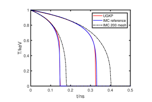
Figure 1: The material temperature $T$ of the Marshak Wave problem for the gray equation of transfer at time $t=10\mathrm{ns}$ and $50\mathrm{ns}$.

In Figure 1, the numerical results of the material temperature at time $t=10\mathrm{ns}$ and $50\mathrm{ns}$ are plotted. The reference solutions are obtained by the implicit Monte Carlo method using $1000$ uniform cells in space. The wavefronts of the UGKP method are consistent with those of the reference solution. Figure 1 also presents the results obtained by the implicit Monte Carlo method using $200$ uniform spatial cells, and it could be seen that for this mesh size, the wavefront of the implicit Monte Carlo method travels faster than the reference solution due to teleportation error. However, the UGKP method does not suffer from the teleportation error because of its asymptotic preserving properties. Therefore, it can use a much larger cell size and time step than the particle mean free path and collision time. For the computation time, the IMC reference solution takes $186$ hours to reach the simulation time of $50\mathrm{ns}$, while the UGKP method takes $8.5$ hours, which demonstrates the UGKP method is more efficient than IMC for this example. The improved efficiency of the UGKP method is because it does not need to compute the large amount of effective scattering employed by the IMC method for this optically thick scenario.

5.2 Frequency-dependent homogeneous problem

The second example we consider is a frequency-dependent homogeneous problem. Initially, radiation and material temperature are equal at $1\mathrm{keV}$, but the specific intensity is not a Planck distribution for frequency. Instead, the initial specific intensity is

$$I_{0}(\boldsymbol{x},\boldsymbol{\Omega},\nu)=\dfrac{acT_{r}^{4}}{4\pi}b(\nu,T_{0}),$$ (5.1)

with $T_{0}=0.1\mathrm{keV}$ and $T_{r}=1\mathrm{keV}$, and $b(\nu,T_{0})$ is the normalized Planck distribution as defined in (3.16). The computation domain is $[0,0.01]\times[0,1]$ with periodic boundary conditions imposed on all boundaries. For this setup, the solution remains constant in space during any arbitrary simulation period, but there is energy exchange between radiation and background material. We take $\sigma$ to be

$$\sigma(\nu,T)=\left\{\begin{array}[]{l}10^{-8}\mathrm{cm}^{-1},\quad\text{if}~{}h\nu\in(0,1),\\[8.53581pt] 1000\mathrm{cm}^{-1},\quad\text{else},\end{array}\right.$$ (5.2)

and the specific heat capacity is set as $0.3\text{GJ}/\text{cm}^{3}/\text{keV}$. Because the absorption coefficient $\sigma$ is almost zero for the low-frequency range, there is little energy exchange between radiation and matter for this range, and the specific intensity is expected to remain close to the initial distribution. For the rest of the frequency range, $\sigma$ is very large, therefore one would expect the final specific intensity to be close to the equilibrium distribution, which is a Planck function associated with the final material temperature. So, we expect the distribution of the specific intensity concerning the frequency variable to evolve into two peaks. This distribution of the specific intensity is a phenomenon unique to the multi-frequency setup, and cannot be captured in the gray approximation to the equation of transfer. In our simulations, a uniform time step of $2.6\times 10^{-4}\mathrm{ns}$ is taken and one mesh grid in space is used.

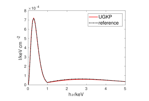
Figure 2: The specific intensity $I$ of the frequency-dependent homogeneous problem at time $t=1\mathrm{ns}$.

In Figure 2, the solution of the specific intensity at $t=1\mathrm{ns}$ with respect to the frequency variable is plotted. The UGKP solution is compared with a reference solution which directly computes the homogeneous problem using multigroup discretization of the frequency variable with $10000$ groups. The UGKP solution and the reference solution are almost identical, showing the capability of the UGKP method to accurately compute frequency-dependent energy exchange. The specific intensity displays two peaks. The left peak is determined by the initial distribution, and the right peak is determined by the final material temperature. The UGKP solution agrees well with our intuition, further verifying the accuracy of this method.

5.3 Frequency-dependent Marshak wave problem

In the third example taken from [39], we consider another Marshak wave problem, but where the opacity depends on frequency. We take the absorption/emission coefficient to be of the form

$$\sigma(\nu,T)=\dfrac{1000}{(h\nu)^{3}\sqrt{kT}},$$ (5.3)

and set the specific heat capacity to be constant at $0.1\mathrm{GJ}/\mathrm{keV}/\mathrm{cm}^{3}$. Initially, the material temperature is $T_{0}=10^{-3}\mathrm{keV}$, and the specific intensity is

$$I_{0}(\boldsymbol{x},\boldsymbol{\Omega},\nu)=B(\nu,T_{0}).$$ (5.4)

The left boundary is kept at a constant specific intensity. Its distribution with respect to the angular variable is isotropic. With respect to the frequency variable, the specific intensity is a Planckian associated with a temperature of $1\mathrm{keV}$. A reflective boundary condition is imposed on the right. This example tests an algorithm’s capability to handle cases where the absorption coefficient varies widely for the whole frequency range. For low frequency where $h\nu$ is small, $\sigma$ can be very large, therefore the system is optically thick. On the other hand, $\sigma$ drops quickly as $h\nu$ increases, and the system becomes optically thin for $h\nu$ surpassing $10\mathrm{keV}$. This multiscale property makes this example a challenging simulation problem.

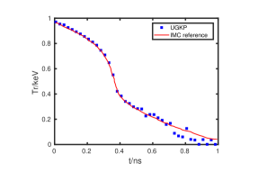
(a) Radiation temperature.

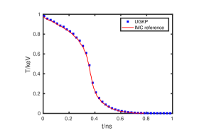
(b) Material temperature.

Figure 3: The radiation and material temperature of the frequency-dependent Marshak Wave problem at time $t=1\mathrm{ns}$.

In our simulations, the computation domain is $[0\mathrm{cm},5\mathrm{cm}]$ and the UGKP method uses a uniform mesh size of $\Delta x=0.005\mathrm{cm}$. The time step is $1.3\times 10^{-4}\mathrm{ns}$. Figure 3 presents the radiation and material temperatures computed by the UGKP method at the simulation time of $1\mathrm{ns}$ and compares them with the IMC solution provided in [39]. The radiation temperature is defined as

$$T_{r}=\sqrt[4]{\dfrac{\rho}{ac}}.$$ (5.5)

A good agreement has been obtained between the UGKP and IMC reference solutions for both the radiation and material temperatures. For this example, the IMC solution in [39] takes $1344$ minutes to reach the simulation time of $1\mathrm{ns}$, while our implementation of the UGKP method takes $349$ minutes. Therefore, the UGKP method is more efficient than the IMC method for this case.

5.4 Marshak wave problem with heterogeneous opacity

The fourth example we consider consists a jump in the absorption coefficient. Within a computation domain of $[0\mathrm{cm},3\mathrm{cm}]$, the function $\sigma(\nu,T)$ takes the following form:

$$\sigma(\nu,T)=\left\{\begin{array}[]{l}\dfrac{10}{(h\nu)^{3}\sqrt{kT}},\quad\text{if}~{}0\mathrm{cm}\leq x\leq 2\mathrm{cm},\\[8.53581pt] \dfrac{1000}{(h\nu)^{3}\sqrt{kT}},\quad\text{else}.\end{array}\right.$$ (5.6)

Therefore, at any arbitrary frequency, there is a discontinuity at the material interface of $x=2\mathrm{cm}$. The radiation always travels through a relatively optically thin region to a relatively optically thick one. The specific heat capacity is held constant at $0.1\mathrm{GJ}/\mathrm{keV}/\mathrm{cm}^{3}$. The initial material temperature is $T_{0}=10^{-3}\mathrm{keV}$. The initial specific intensity is isotropic with respect to the angular variable and a Planckian at $T_{0}$ with respect to frequency. The specific intensity on the left boundary is kept constant at an isotropic angular distribution and a Planckian frequency distribution associated with a temperature of $1\mathrm{keV}$. A reflective boundary condition is imposed on the right boundary. This example tests a method’s ability to treat discontinuity in opacity.

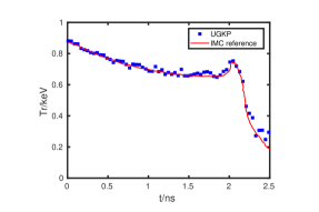
(a) Radiation temperature.

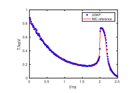
(b) Material temperature.

Figure 4: The radiation and material temperature of the frequency-dependent Marshak Wave problem with heterogeneous opacity at time $t=1\mathrm{ns}$.

The UGKP method uses a uniform mesh size of $\Delta x=0.005\mathrm{cm}$. The time step is taken to be $1.3\times 10^{-4}\mathrm{ns}$. Figure 4 compares the material and radiation temperatures computed by the UGKP method with the IMC solution provided in [39] at the simulation time of $1\mathrm{ns}$, and good agreement could be observed. For this example, the IMC solution in [39] takes $363$ minutes to reach the simulation time of $1\mathrm{ns}$, while our implementation of the UGKP method takes $121$ minutes, showing the UGKP method to be more efficient than the IMC method for this case.

5.5 A hohlraum problem for the gray equation of transfer

For the fifth example, we study the hohlraum problem for the gray equation of transfer. This problem describes the heating of a cavity by a radiation source. It is of wide interest in the literature and has also been studied in [26, 35].

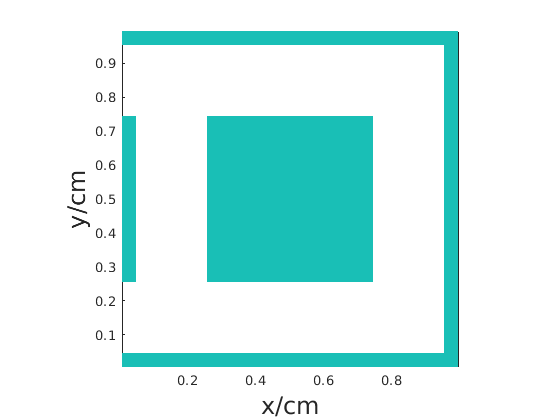
Figure 5: The layout of the hohlraum problem for the gray equation of transfer. The green regions are where $(x,y)\in[0,0.05]\times[0.25,0.75]$, and $(x,y)\in[0.25,0.75]\times[0.25,0.75]$, $(x,y)\in[0,1]\times[0,0.05]$, $(x,y)\in[0,1]\times[0.95,1]$ and $(x,y)\in[0.95,1]\times[0,1]$.

The layout of the problem is shown in Figure 5. The white region within the computation domain of $[0\mathrm{cm},1\mathrm{cm}]\times[0\mathrm{cm},1\mathrm{cm}]$ is a vacuum. In our simulation, we take an absorption coefficient of $\sigma=10^{-8}\mathrm{cm}^{-1}$ and a specific heat capacity of $C_{v}=10^{-4}\mathrm{GJ}/\mathrm{keV}/\mathrm{cm}^{3}$ for this region. The green regions are filled with material satisfying $\sigma=\dfrac{100}{(T/T_{\mathrm{keV}})^{3}}\mathrm{cm}^{-1}$, where $T_{\mathrm{keV}}=1\mathrm{keV}$. The specific heat capacity $C_{v}$ for the green regions are $0.3\mathrm{GJ}/\mathrm{keV}/\mathrm{cm}^{3}$. The initial material temperature is uniform at $10^{-3}\mathrm{keV}$. The radiation and material temperatures are initially at equilibrium. The initial specific intensity is isotropic in the angular variable and a Planckian in the frequency variable. The entire left boundary is kept constant with an angularly isotropic specific intensity of $1\mathrm{keV}$ black body source. The reflective boundary is imposed on the right. The upper and lower boundaries are kept constant at a specific intensity which is a Planckian corresponding to a temperature of $10^{-3}\mathrm{keV}$.

For this problem, the material is initially cold and therefore optically thick. Its opacity decreases as radiation heat up the material. Therefore, the absorption coefficient varies over a wide range in time and space. The presence of a vacuum in the computation domain further complicates the problem and makes it even more challenging. It was shown [26] that for this problem, the diffusion approximation could not capture the correct physics, and therefore it is necessary to simulate the original radiative transfer equation (2.1).

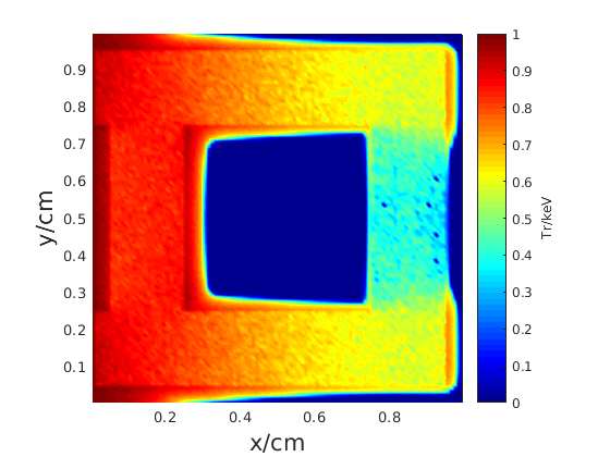
(a) Radiation temperature.

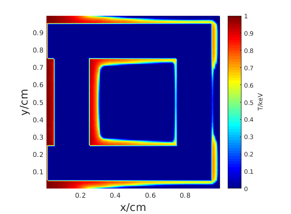
(b) Material temperature.

Figure 6: The radiation and material temperatures of the hohlraum problem for the gray equation of transfer at time $t=1\mathrm{ns}$.

The UGKP method uses a uniform spatial mesh of $100\times 100$, and the time step is taken to be $2.7\times 10^{-4}\mathrm{ns}$. Figure 6 presents the contour plots of the UGKP solution for the radiation temperature and the material temperature at the simulation time $1\mathrm{ns}$. Our solutions are in general agreement with the solutions presented in [26, 35]. Also, it has been stated in [26] that for this problem, the solution should preserve two properties: firstly, there should be a non-uniform heating of the central block. Secondly, there should be less radiation directly behind the block than those regions within sight of the source. The UGKP solutions satisfy these two properties, verifying the accuracy of our method.

5.6 Frequency-dependent hohlraum problem

The final example we present is the hohlraum problem for the multi-frequency radiative transfer equation. The setup of this problem is the same as that studied in [8]. The layout of this problem is shown in Figure 7. The computation domain is $[0\mathrm{cm},0.65\mathrm{cm}]\times[0\mathrm{cm},1.4\mathrm{cm}]$. The white region within the computation domain is almost a vacuum, and we take the absorption coefficient to be $\sigma=10^{-8}\mathrm{cm}^{-1}$ and the specific heat capacity $C_{v}$ to be $10^{-4}\mathrm{GJ}/\mathrm{keV}/\mathrm{cm}^{3}$. The green regions have a frequency-dependent opacity with the form

$$\sigma(\nu,T)=\dfrac{1000(1-\mathrm{e}^{-\frac{h\nu}{kT}})}{(h\nu)^{3}}.$$ (5.7)

The specific heat capacity within the green regions is $C_{v}=0.3\mathrm{GJ}/\mathrm{keV}/\mathrm{cm}^{3}$. The initial material temperature is $T_{0}=10^{-3}\mathrm{keV}$, and radiation and material are initially at equilibrium. Therefore, the initial specific intensity is

$$I_{0}(\boldsymbol{x},\boldsymbol{\Omega},\nu)=B(\nu,T_{0}).$$ (5.8)

The reflective boundary condition is imposed on the left boundary. The lower boundary is kept constant with an angularly isotropic specific intensity of $0.3\mathrm{keV}$ black body source. The upper and right boundaries are kept constant at a specific intensity which is a Planckian corresponding to a temperature of $10^{-3}\mathrm{keV}$.

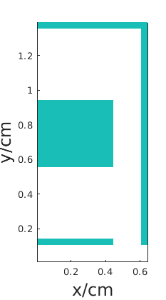
Figure 7: The layout of the hohlraum problem for the frequency-dependent equation of transfer. The green regions are where $(x,y)\in[0,0.45]\times[0.1,0.15]$, and $(x,y)\in[0,0.45]\times[0.55,0.95]$, $(x,y)\in[0.6,0.65]\times[0.1,1.4]$, and $(x,y)\in[0,0.65]\times[1.35,1.4]$.

This problem is even more complicated than the hohlraum problem for the gray equation of transfer studied in Section 5.5, as the material opacity depends on frequency. For low frequency, the material is optically thick, but for the higher frequency it becomes optically thin, and the opacity varies widely within the whole frequency range. The presence of the vacuum in the computation domain and the fact the opaque walls within the cavity are sometimes very narrow further complicates the problem, making it a very challenging benchmark.

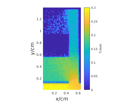
(a) Radiation temperature.

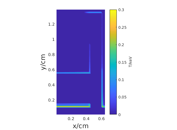
(b) Material temperature.

Figure 8: The radiation and material temperature of hohlraum problem for the frequency-dependent equation of transfer at time $t=10\mathrm{ns}$.

In computing this example, a limiter is employed to suppress artificial oscillations at material interfaces. Based on similar considerations as [45], we define

$$\tau=\dfrac{\epsilon^{2}}{c\sigma}+10\Delta t\dfrac{T_{l}-T_{r}}{T_{l}+T_{r}}\dfrac{2}{\Delta x_{l}+\Delta x_{r}}$$ (5.9)

at material interfaces. In (5.9), $T_{l}$, $T_{r}$, and $\Delta x_{l}$, $\Delta x_{r}$ are the left and right values of material temperature and grid length on both sides of the interface. In computing the distance to absorption for particles crossing the interface, equation (3.10) is replaced by

$$d_{\mathrm{COL}}=c|\ln\xi|\tau.$$ (5.10)

For computing the macroscopic solver, $\kappa^{eff}$ in equation (3.39) is multiplied by a factor of

$$f=\dfrac{1-\exp\left(-\Delta t/\tau\right)}{1-\exp\left(-c\sigma\Delta t/\epsilon^{2}\right)}.$$ (5.11)

We note that this limiter is only applied to material interfaces where there is a large jump in material temperature, and does not affect the asymptotic preserving properties of the UGKP method.

The UGKP method uses a uniform spatial mesh of $52\times 112$, and the time step is taken to be $1.7\times 10^{-4}\mathrm{ns}$. The contour plots of the UGKP solution for the radiation temperature and the material temperature at the simulation time $10\mathrm{ns}$ are shown in Figure 8. The UGKP solutions are in rough agreement with the solutions presented in [8], verifying the accuracy of our method. Also, we observe a smooth material temperature profile, both at the lower wall and the lower side of the center block, which shows that unlike the deterministic particle method discussed in [8], the UGKP method does not suffer from ray effects. The UGKP solution for the radiation temperature also does not show ray effects [28], though the solution is noisier than the solutions presented in [8].

6 Conclusions

We have extended the unified gas-kinetic particle method (UGKP) studied previously in [20, 34] to multi-frequency radiative transfer. Particle sampling combined with analytical representation of the specific intensity’s reliance on frequency enables our method to preserve the Rosseland diffusion limit. Compared with the implicit Monte Carlo method, our method does not track particle trajectory after first collision event, therefore a high efficiency is obtained. Numerical analysis shows that our UKGP method is asymptotic preserving for both free-streaming and diffusion limit. We demonstrate with numerical examples the accuracy and efficiency of the proposed UGKP method for benchmark problems where there is a wide variation of opacity. Future works includes extension to arbitrary quadrilateral mesh and cylindrical geometries.

References

- [1] Marvin L Adams and Edward W Larsen. Fast iterative methods for discrete-ordinates particle transport calculations. Progress in nuclear energy, 40(1):3–159, 2002.
- [2] Luis Chacon, Guangye Chen, Dana A Knoll, C Newman, H Park, William Taitano, Jeff A Willert, and Geoffrey Womeldorff. Multiscale high-order/low-order (HOLO) algorithms and applications. Journal of Computational Physics, 330:21–45, 2017.
- [3] Jeffery D Densmore. Asymptotic analysis of the spatial discretization of radiation absorption and re-emission in Implicit Monte Carlo. Journal of Computational Physics, 230(4):1116–1133, 2011.
- [4] Joseph A Fleck Jr and JD Cummings Jr. An implicit Monte Carlo scheme for calculating time and frequency dependent nonlinear radiation transport. Journal of Computational Physics, 8(3):313–342, 1971.
- [5] Yanqi Gao, Yong Cui, Lailin Ji, Daxing Rao, Xiaohui Zhao, Fujian Li, Dong Liu, Wei Feng, Lan Xia, Jiani Liu, et al. Development of low-coherence high-power laser drivers for inertial confinement fusion. Matter and Radiation at Extremes, 5(6):065201, 2020.
- [6] Zhaoli Guo and Kun Xu. Progress of discrete unified gas-kinetic scheme for multiscale flows. Advances in Aerodynamics, 3(1):1–42, 2021.
- [7] Zhaoli Guo, Kun Xu, and Ruijie Wang. Discrete unified gas kinetic scheme for all Knudsen number flows: Low-speed isothermal case. Physical Review E, 88(3):033305, 2013.
- [8] Hans Hammer, HyeongKae Park, and Luis Chacon. A multi-dimensional, moment-accelerated deterministic particle method for time-dependent, multi-frequency thermal radiative transfer problems. Journal of Computational Physics, 386:653–674, 2019.
- [9] Shi Jin. Efficient asymptotic-preserving (AP) schemes for some multiscale kinetic equations. SIAM Journal on Scientific Computing, 21(2):441–454, 1999.
- [10] Shi Jin. Asymptotic preserving (AP) schemes for multiscale kinetic and hyperbolic equations: a review. Lecture notes for summer school on methods and models of kinetic theory (M&MKT), Porto Ercole (Grosseto, Italy), pages 177–216, 2010.
- [11] N Jourdain, U Chaulagain, M Havlík, D Kramer, D Kumar, I Majerová, VT Tikhonchuk, G Korn, and S Weber. The l4n laser beamline of the P3-installation: Towards high-repetition rate high-energy density physics at ELI-Beamlines. Matter and Radiation at Extremes, 6(1):015401, 2021.
- [12] Dongdong Kang, Yong Hou, Qiyu Zeng, and Jiayu Dai. Unified first-principles equations of state of deuterium-tritium mixtures in the global inertial confinement fusion region. Matter and Radiation at Extremes, 5(5):055401, 2020.
- [13] Kendra P Keady and Mathew A Cleveland. An improved random walk algorithm for the implicit Monte Carlo method. Journal of Computational Physics, 328:160–176, 2017.
- [14] Ke Lan. Dream fusion in octahedral spherical hohlraum. Matter and Radiation at Extremes, 7(5):055701, 2022.
- [15] Edward Larsen. A grey transport acceleration method far time-dependent radiative transfer problems. Journal of Computational Physics, 78(2):459–480, 1988.
- [16] Edward W Larsen, Akansha Kumar, and Jim E Morel. Properties of the implicitly time-differenced equations of thermal radiation transport. Journal of Computational Physics, 238:82–96, 2013.
- [17] EW Larsen, GC Pomraning, and VC Badham. Asymptotic analysis of radiative transfer problems. Journal of Quantitative Spectroscopy and Radiative Transfer, 29(4):285–310, 1983.
- [18] CD Levermore and GC Pomraning. A flux-limited diffusion theory. The Astrophysical Journal, 248:321–334, 1981.
- [19] Ruo Li, Peng Song, and Lingchao Zheng. A nonlinear moment model for radiative transfer equation. Multiscale Modeling & Simulation, 19(3):1425–1452, 2021.
- [20] Weiming Li, Chang Liu, Yajun Zhu, Jiwei Zhang, and Kun Xu. Unified gas-kinetic wave-particle methods III: Multiscale photon transport. Journal of Computational Physics, 408:109280, 2020.
- [21] Chang Liu and Kun Xu. Unified gas-kinetic wave-particle methods iv: Multi-species gas mixture and plasma transport. Advances in Aerodynamics, 3(1):1–31, 2021.
- [22] Chang Liu, Guangzhao Zhou, Wei Shyy, and Kun Xu. Limitation principle for computational fluid dynamics. Shock Waves, 29(8):1083–1102, 2019.
- [23] Chang Liu, Yajun Zhu, and Kun Xu. Unified gas-kinetic wave-particle methods I: Continuum and rarefied gas flow. Journal of Computational Physics, 401:108977, 2020.
- [24] Peter G Maginot, Jean C Ragusa, and Jim E Morel. High-order solution methods for grey discrete ordinates thermal radiative transfer. Journal of Computational Physics, 327:719–746, 2016.
- [25] Lucio Mayer, Graeme Lufkin, Thomas Quinn, and James Wadsley. Fragmentation of gravitationally unstable gaseous protoplanetary disks with radiative transfer. The Astrophysical Journal, 661(1):L77, 2007.
- [26] Ryan G McClarren and Cory D Hauck. Robust and accurate filtered spherical harmonics expansions for radiative transfer. Journal of Computational Physics, 229(16):5597–5614, 2010.
- [27] J. E. Morel. A synthetic acceleration method for discrete ordinates calculations with highly anisotropic scattering. Nuclear Science and Engineering, 82(1):34–46, 1982.
- [28] J. E. Morel, T. A. Wareing, R. B. Lowrie, and D. K. Parsons. Analysis of ray-effect mitigation techniques. Nuclear Science and Engineering, 144(1):1–22, 2003.
- [29] Olena Palii and Matthias Schlottbom. On a convergent DSA preconditioned source iteration for a DGFEM method for radiative transfer. Computers & Mathematics with Applications, 79(12):3366–3377, 2020.
- [30] Gaël Poëtte and Xavier Valentin. A new implicit monte-carlo scheme for photonics (without teleportation error and without tilts). Journal of Computational Physics, 412:109405, 2020.
- [31] Gerald C Pomraning. The equations of radiation hydrodynamics. Courier Corporation, 2005.
- [32] Martin Philip Sherman. Moment methods in radiative transfer problems. Journal of Quantitative Spectroscopy and Radiative Transfer, 7(1):89–109, 1967.
- [33] Yi Shi, Xiaole Han, Wenjun Sun, and Peng Song. A continuous source tilting scheme for radiative transfer equations in implicit Monte Carlo. Journal of Computational and Theoretical Transport, 50(1):1–26, 2020.
- [34] Yi Shi, Peng Song, and WenJun Sun. An asymptotic preserving unified gas kinetic particle method for radiative transfer equations. Journal of Computational Physics, 420:109687, 2020.
- [35] Elad Steinberg and Shay I Heizler. Multi-frequency implicit semi-analog Monte-Carlo (ISMC) radiative transfer solver in two-dimensions (without teleportation). Journal of Computational Physics, 450:110806, 2022.
- [36] Wei Su, Lianhua Zhu, Peng Wang, Yonghao Zhang, and Lei Wu. Can we find steady-state solutions to multiscale rarefied gas flows within dozens of iterations? Journal of Computational Physics, 407:109245, 2020.
- [37] Wenjun Sun, Song Jiang, and Kun Xu. An asymptotic preserving unified gas kinetic scheme for gray radiative transfer equations. Journal of Computational Physics, 285:265–279, 2015.
- [38] Wenjun Sun, Song Jiang, and Kun Xu. An asymptotic preserving implicit unified gas kinetic scheme for frequency-dependent radiative transfer equations. International Journal of Numerical Analysis & Modeling, 15, 2018.
- [39] Wenjun Sun, Song Jiang, Kun Xu, and Shu Li. An asymptotic preserving unified gas kinetic scheme for frequency-dependent radiative transfer equations. Journal of Computational Physics, 302:222–238, 2015.
- [40] Min Tang, Li Wang, and Xiaojiang Zhang. Accurate front capturing asymptotic preserving scheme for nonlinear gray radiative transfer equation. SIAM Journal on Scientific Computing, 43(3):B759–B783, 2021.
- [41] Stuart C Whitehouse and Matthew R Bate. Smoothed particle hydrodynamics with radiative transfer in the flux-limited diffusion approximation. Monthly Notices of the Royal Astronomical Society, 353(4):1078–1094, 2004.
- [42] Ryan T Wollaeger, Daniel R van Rossum, Carlo Graziani, Sean M Couch, George C Jordan IV, Donald Q Lamb, and Gregory A Moses. Radiation transport for explosive outflows: A multigroup hybrid Monte Carlo method. The Astrophysical Journal Supplement Series, 209(2):36, 2013.
- [43] Lei Wu, Jun Zhang, Haihu Liu, Yonghao Zhang, and Jason M Reese. A fast iterative scheme for the linearized Boltzmann equation. Journal of Computational Physics, 338:431–451, 2017.
- [44] Tao Xiong, Wenjun Sun, Yi Shi, and Peng Song. High order asymptotic preserving discontinuous Galerkin methods for gray radiative transfer equations. Journal of Computational Physics, page 111308, 2022.
- [45] Kun Xu. A gas-kinetic BGK scheme for the Navier–Stokes equations and its connection with artificial dissipation and Godunov method. Journal of Computational Physics, 171(1):289–335, 2001.
- [46] Kun Xu and Juan-Chen Huang. A unified gas-kinetic scheme for continuum and rarefied flows. Journal of Computational Physics, 229(20):7747–7764, 2010.