Stabilized cut discontinuous Galerkin methods for advection-reaction problems on surfaces

Abstract

We develop a novel cut discontinuous Galerkin (CutDG) method for stationary advection-reaction problems on surfaces embedded in $\mathbb{R}^{d}$. The CutDG method is based on embedding the surface into a full-dimensional background mesh and using the associated discontinuous piecewise polynomials of order $k$ as test and trial functions. As the surface can cut through the mesh in an arbitrary fashion, we design a suitable stabilization that enables us to establish inf-sup stability, a priori error estimates, and condition number estimates using an augmented streamline-diffusion norm. The resulting CutDG formulation is geometrically robust in the sense that all derived theoretical results hold with constants independent of any particular cut configuration. Numerical examples support our theoretical findings.

1 Introduction

1.1 Background and earlier work

Advection-dominated transport processes on surfaces appear in many important phenomena in science and engineering. Prominent applications include flow and transport problems in porous media when large-scale fracture networks are modeled as composed 2D surfaces embedded into a 3D bulk domain [1, 2, 3, 4]. Another important instance arises when modeling incompressible multi-phase flow problems with surfactants [5, 6, 7, 8], where potentially low surface diffusion coefficients lead to large surface Péclet numbers [9] in the surface-bounded surfactants transport model. Numerical methods for these applications must not only remain stable and accurate when solving the underlying partial differential equations (PDEs) in the advection-dominant regime, but preferably should also be able to handle complicated and evolving surface geometries with ease. As a potential remedy, unfitted finite element methods known as cut finite element methods (CutFEM) [10, 11] or TraceFEMs [12] have been developed for the last 13 years which allow for more flexible handling of surface geometries by embedding them into a structured and easy-to-generate background mesh which does not fit the surface geometry. For the development of more classical fitted Surface Finite Element Methods (SFEM) initiated in the seminal work [13], we refer to the excellent and comprehensive reviews [14, 15].

Using continuous piecewise linear finite element functions from the ambient space, the first unfitted finite element method for elliptic problems on surfaces was proposed in [12], and later extended to higher-order elements in [16, 17]. As the embedded surface geometry can cut through the background mesh in an arbitrary fashion, one main challenge in devising unfitted finite element methods is to ensure their geometrical robustness in the sense that they satisfy similar stability, a priori error, and conditioning number estimates as their fitted mesh counterparts, but with constants that are independent of the particular cut configuration. A rather universal approach to achieving geometrical robustness is to augment the weak formulation under consideration with suitably designed stabilizations also known as ghost penalties [10]. For Laplace-Beltrami-type problems on surfaces, ghost penalties based on face stabilization and artificial diffusion were introduced in [18] and [19], respectively. The contributions from [20, 21] then proposed an abstract stabilization CutFEM framework to discretize elliptic problems using continuous higher-order elements as well as on embedded manifolds of co-dimension larger than one. In particular, the volume normal gradient stabilization introduced in [20, 21] was then successfully used to weakly enforce the tangential condition in vector-valued problems including the surface Darcy equation [22] and the surface Stokes equation [23, 24], all resting upon continuous finite elements.

So far, most fitted and unfitted finite element schemes for surface PDEs have been designed for diffusion-dominated elliptic or parabolic type problems [25, 26, 27, 28, 29, 30, 31], in contrast to the plethora of both stabilized continuous and discontinuous Galerkin schemes for advection-dominated problems posed in the Euclidian flat case, see for instance the comprehensive monograph [32] or the recent textbook [33]. Interestingly, relevant work on advection-dominated surface problems appeared first in the context of unfitted finite elements, starting with [34], where the classical Streamline Upwind Petrov–Galerkin (SUPG) approach was combined with TraceFEM. Later [35] considered a characteristic CutFEM for convection-diffusion problems on time-dependent surfaces. Moreover, CutFEM formulations for advection-dominated problems on surfaces have been proposed using the continuous interior penalty method [36], an artificial diffusion/full-gradient approach [4], and a normal-gradient stabilized streamline-line diffusion approach [37]. Finally, an adaptive TraceFEM formulation with mesh adaption guided by a posteriori error estimators was developed in [38] to solve potentially advection-dominated advection-diffusion-reaction problems. Regarding fitted mesh-based approaches on explicitly triangulated surfaces, variants employing local projection stabilization [39, 40] and Petrov–Galerkin type techniques [41, 42] can be found in the literature.

The development of discontinuous Galerkin (DG) methods for hyperbolic and advection-dominated problems was initiated [43], with the first theoretical analyses being presented in [44, 45]. Later, [46] reformulated and generalized the upwind flux strategy in DG methods by introducing a tunable stabilization parameter. The advantageous conservation and stability properties, the high locality, and the naturally inherited upwind flux term in the bilinear form make DG methods popular to handle specifically advection-dominated problems [47, 48, 49] as well as elliptic ones [50, 51]. Detailed overviews are provided by the monographs [52, 53]. In contrast, the development of DG methods for advection-dominated problems on surfaces has been almost completely neglected. Only the unpublished preprint [54] proposes a DG formulation for advection-dominated problems on surfaces using piecewise linear elements on fitted meshes, but the presented formulation contains a geometrically inconsistent velocity-related term leading to suboptimal error estimates. To the best of our knowledge, mostly elliptic problems have been considered in the context of DG methods, see, e.g., [55, 56] and [57] for respectively primal and mixed formulations of the Poisson surface problem on fitted meshes, while [58] proposed a stabilized unfitted cut discontinuous Galerkin method (CutDG) based on first-order elements and symmetric interior penalties. The latter was then combined in [59, 60] with a CutDG method for bulk problems to discretize elliptic bulk-surface problems. The general stabilization approach is in contrast to alternative unfitted discontinuous Galerkin methods for bulk PDEs [61, 62, 63, 64, 65, 66, 67, 68], where troublesome small cut elements are merged with neighbor elements with a large intersection support by simply extending the local shape functions from the large element to the small cut element. While the cell-merging approach automatically upholds local conservation properties of the original scheme, some drawbacks exist including the almost complete absence of numerical analysis except for [69, 70], and, most importantly for the present contribution, the lack of natural extension to surface PDEs. More specifically, unfitted finite element methods for surface PDEs do not only suffer from the classical small cut element problem, but more importantly, the linear dependency of local shape functions when restricted to a lower-dimensional manifold poses the most significant challenge which cannot be addressed by a purely cell-merging based approach.

1.2 New contributions and outline of the paper

In this work, we present a new cut discontinuous Galerkin (CutDG) method for the discretization of stationary advection-reaction problems on embedded surfaces. This contribution is part of our long-term efforts to develop a fully-fledged, stabilized cut discontinuous Galerkin (CutDG) framework for the discretization of complex multi-physics interface problems initiated in [58, 71, 72]. Our main motivation is that the stabilization approach provides us with a versatile theoretical and practical road to formulate, analyze and implement unfitted discontinuous Galerkin methods. The presented approach draws inspiration from our earlier contributions [58, 72], but compared to [58], we shift here our focus from pure diffusion problems to advection-reaction problems while also considering higher-order elements. In contrast to our work [72] on CutDG methods for advection-reaction bulk problems, we need here to develop new stabilization for the surface-bound PDE. Such a task is not a straightforward extension of our techniques developed in [72] as additional stability issues arise in the surface case which are not present in the bulk version. Moreover, we also provide precise estimates of all geometrical errors caused by the geometric approximation of the surface.

We start by briefly recalling the advection-reaction model problem on surfaces and the corresponding weak formulations in Section 2, followed by a presentation of the proposed CutDG method in Section 3. Our approach departs from an embedding of the surface $\Gamma$ into a higher dimensional background mesh ${\mathcal{T}}_{h}$. To account for geometrical errors typically occurring in surface PDE discretizations, we only assume that a piecewise polynomial approximation $\Gamma_{h}$ of order $k_{g}$ is available so that the errors in position and normal are $O(h^{k_{g}+1})$ and $O(h^{k_{g}})$, respectively. On the discrete surface $\Gamma_{h}$ we formulate a discontinuous Galerkin method which closely resembles the classical upwind formulation presented in [46], but uses the discrete function spaces stemming from the background mesh. The resulting formulation is highly ill-posed due to a) the potential small intersection between mesh elements and surface discretization and, more importantly, b) the arising linear dependency of local 3D shape functions when restricted to the 2D surface. We like to point out that the popular cell-merging approach for unfitted DG methods for bulk problems does not provide a remedy for b). Instead, we add a consistent stabilization $s_{h}$ to the surface bounded bilinear form $a_{h}$, which renders the method geometrically robust and enables us to prove inf-sup stability and optimal convergence for our CutDG method with respect to a combined stabilized upwind flux/streamline diffusion-type norm which is independent of the particular cut configuration. Our stabilization framework works automatically for higher-order approximation spaces with polynomial orders $k$ and is not limited to low-order schemes. After collecting several auxiliary results regarding norms, interpolation operators, and geometry-related error estimates in Section 4, we provide a detailed motivation and derivation of a suitable stabilization operator for our CutDG method in Section 5. Extending the approaches from [58, 21, 72], we prove that a properly scaled normal gradient volume stabilization together with low-order jump terms gives us control of certain rescaled upwind and streamline diffusion norms which are evaluated on the full background mesh. As a result, we can show that our formulation satisfies a geometrically robust inf-sup condition with respect to the stabilized streamline diffusion norm. The subsequent a priori error analysis in Section 6 builds upon the classical Strang-type lemma approach which decomposed the total error into a best approximation error, a consistency error caused by the stabilization, and a geometrical error arising from the surface approximation. For each contribution, detailed estimates are given. Afterward, we demonstrate in Section 7 that thanks to our stabilization, the condition number of the resulting system matrix scales exactly as the corresponding fitted DG upwind formulation in the flat Euclidian case. Finally, we corroborate our theoretical findings with a series of numerical experiments in Section 8 where we study both the convergence properties and geometrical robustness of the proposed CutDG method.

2 Model problem

2.1 Basic notation

In this work, we let $\Gamma$ be a compact, oriented, and smooth hypersurface without boundary, embedded in $\mathbb{R}^{d}$ and equipped with a smooth normal field $n:\Gamma\rightarrow\mathbb{R}^{d}$. Let $\rho$ denote the signed distance function that measures the distance in the normal direction from $\Gamma$, defined on a $\delta$-neighborhood $U_{\delta}(\Gamma)=\{x\in\mathbb{R}^{d}\mid\text{dist}(x,\Gamma)<\delta\}$, see Figure 3.1 (left). Then it is well-known that the closest point projection $p:U_{\delta}(\Gamma)\rightarrow\Gamma$ implicitly defined by

$$p(x)=x-\rho(x)n(p(x))$$ (2.1)

is well-defined in $U_{\delta}(\Gamma)$ provided that $\delta<\kappa^{-1}$, where $\kappa=\max_{i=1,\ldots,d-1}\|\kappa_{i}\|_{L^{\infty}(\Gamma)}$ is the maximum of the principal curvatures of $\Gamma$. Using the closest point projection we can define the extension $u^{e}$ of a function, $u$ defined on $\Gamma$ to the $\delta$-neighborhood $U_{\delta}(\Gamma)$ by setting

$$u^{e}(x)=u(p(x)).$$ (2.2)

Conversely, a function $w$ defined on a subset $\widetilde{\Gamma}\subset U_{\delta}(\Gamma)$ can be lifted back to $p(\widetilde{\Gamma})\subset\Gamma$ via

$$w^{l}(x)=w(p^{-1}(x)),$$ (2.3)

whenever the closest point mapping $p:\widetilde{\Gamma}\to p(\widetilde{\Gamma})$ is bijective. Then

$$(w^{l}(x))^{e}=w^{l}(p(x))=w\circ p^{-1}\circ p(x)=w.$$ (2.4)

Furthermore, for a function $u:\Gamma\rightarrow\mathbb{R}$, we define the tangential gradient $\nabla_{\Gamma}$ on $\Gamma$ by

$$\nabla_{\Gamma}u=P_{\Gamma}\nabla u^{e}.$$ (2.5)

The operator $P_{\Gamma}=P_{\Gamma}(x)$ is the orthogonal projection of $\mathbb{R}^{d}$ onto the tangent space of $\Gamma$ at $x\in\Gamma$ given by

$$P_{\Gamma}=I-n_{\Gamma}\otimes n_{\Gamma},$$ (2.6)

where $I$ is the identity matrix. For a vector field $v$ on $\Gamma$, the tangential divergence is defined as

$$\nabla_{\Gamma}\cdot v=\nabla\cdot v-n_{\Gamma}\cdot\nabla vn_{\Gamma}.$$ (2.7)

For any sufficient regular subset $U\subseteq\mathbb{R}^{d}$ and $0\leqslant m<\infty$, $1\leqslant q\leqslant\infty$, we denote by $W^{m,q}(U)$ the standard Sobolev spaces consisting of those $\mathbb{R}$-valued functions defined on $U$ which possess $L^{q}$-integrable weak derivatives up to order $m$. Their associated norms are denoted by $\|\cdot\|_{m,q,U}$. As usual, we write $H^{m}(U)=W^{m,2}(U)$ and $(\cdot,\cdot)_{m,U}$ and $\|\cdot\|_{m,U}$ for the associated inner product and norm. If unmistakable, we occasionally write $(\cdot,\cdot)_{U}$ and $\|\cdot\|_{U}$ for the inner products and norms associated with $L^{2}(U)$, with $U$ being a measurable subset of $\mathbb{R}^{d}$. Any norm $\|\cdot\|_{\mathcal{P}_{h}}$ used in this work which involves a collection of geometric entities $\mathcal{P}_{h}$ should be understood as the broken norm defined by $\|\cdot\|_{\mathcal{P}_{h}}^{2}=\sum_{P\in\mathcal{P}_{h}}\|\cdot\|_{P}^{2}$ whenever $\|\cdot\|_{P}$ is well-defined, with a similar convention for scalar products $(\cdot,\cdot)_{\mathcal{P}_{h}}$. Any set operations involving $\mathcal{P}_{h}$ are also understood as element-wise operations, e.g., $\mathcal{P}_{h}\cap U=\{P\cap U\;|\;P\in\mathcal{P}_{h}\}$ and $\partial\mathcal{P}_{h}=\{\partial P\;|\;P\in\mathcal{P}_{h}\}$ allowing for a compact short-hand notation such as $(v,w)_{\mathcal{P}_{h}\cap U}=\sum_{P\in\mathcal{P}_{h}}(v,w)_{P\cap U}$ and $\|\cdot\|_{\partial\mathcal{P}_{h}\cap U}=\sqrt{\sum_{P\in\mathcal{P}_{h}}\|\cdot\|_{\partial P\cap U}^{2}}$. Moreover, for geometric entities $P$ of Hausdorff dimension $l$, we denote their $l$-dimensional Hausdorff measure by $|P|_{l}$. Finally, throughout this work, we use the notation $a\lesssim b$ for $a\leqslant Cb$ for some generic constant $C$ (even for $C=1$) which varies with the context but is always independent of the mesh size $h$ and the position of $\Gamma$ relative to the background $\mathcal{T}_{h}$, but may depend on the dimension $d$, the polynomial degree of the finite element functions, the shape regularity of the mesh, and the curvature of $\Gamma$. The binary relations $\gtrsim$ and $\sim$ are defined analogously.

2.2 The continuous problem

We consider the following advection-reaction problem on a surface: find $u:\Gamma\rightarrow\mathbb{R}$ such that

$$b\cdot\nabla_{\Gamma}u+cu=f\text{ on }\Gamma,$$ (2.8)

where $b\in[W^{1,\infty}(\Gamma)]^{d}$ is a given vector field, and $c\in L^{\infty}(\Gamma)$ and $f\in L^{2}(\Gamma)$ are given scalar function. The corresponding weak form is: find $u\in V=\{v\in L^{2}(\Gamma)\;|\;b\cdot\nabla_{\Gamma}v\in L^{2}(\Gamma)\}$ such that

$$a(u,v)=l(v)\hskip 14.22636pt\forall v\in V,$$ (2.9)

with the bilinear form $a(\cdot,\cdot)$ and the linear form $l(\cdot)$ being given by

$$a(u,v) =(b\cdot\nabla_{\Gamma}u+cu,v)_{\Gamma},$$

$$l(v) =(f,v)_{\Gamma}.$$ (2.10)

Furthermore, to ensure that problem (2.8) is well-posed, we assume as usual that

$$\operatorname*{ess\,inf}_{x\in\Gamma}\big{(}c(x)-\frac{1}{2}\nabla_{\Gamma}\cdot b(x)\big{)}\geqslant c_{0}>0,$$ (2.11)

for some positive constant $c_{0}$.

3 Stabilized cut discontinuous Galerkin methods

3.1 Computational domains and discrete function spaces

Let $\{\widetilde{\mathcal{T}}_{h}\}_{h}$ be a family of quasi-uniform meshes consisting of shape-regular elements $T$ with element diameter $h_{T}<\delta$ covering the $\delta$ neighborhood $U_{\delta}(\Gamma)$ of the surface $\Gamma$. For simplicity, we assume that our mesh consists of either simplicial or cubic elements of dimension $d$. In computations, one typically does not have an exact representation of the surface $\Gamma$, but rather an approximation $\Gamma_{h}$. In this work, the discrete surface $\Gamma_{h}$ is supposed to satisfy the following assumptions:

• $\Gamma_{h}\subset U_{\delta}(\Gamma)$ and the closest point mapping $p:\Gamma_{h}\rightarrow\Gamma$ is a bijection for $0<h\leqslant h_{0}$.

• The following estimates hold

  $$\|\rho\|_{L^{\infty}(\Gamma_{h})}\lesssim h^{k_{g}+1},\qquad\|n^{e}-n_{h}\|_{L^{\infty}(\Gamma_{h})}\lesssim h^{k_{g}}$$ (3.1)

  for a positive integer $k_{g}\geqslant 1$.

Typically, the distance function $\rho$ is approximated by its interpolation $\rho_{h}=I_{h}^{k_{g}}\rho$ into the space of continuous, piecewise polynomials of order $k_{g}$ on $\mathcal{T}_{h}$. Then the discrete surface $\Gamma_{h}$ given as the zero level set of $\rho_{h}$ satisfies the assumptions in equation (3.1).

For a given background mesh $\widetilde{\mathcal{T}}_{h}$ and discrete surface $\Gamma_{h}$, the active mesh $\mathcal{T}_{h}$ is defined as the collection of those mesh elements that have a nonempty intersection with the discrete surface,

$$\mathcal{T}_{h}=\{T\in\widetilde{\mathcal{T}}_{h}\mid T\cap\Gamma_{h}\neq\emptyset\},$$ (3.2)

while the union of all the active elements is denoted by

$$\mathcal{N}_{h}=\bigcup_{T\in\mathcal{T}_{h}}T.$$ (3.3)

Further, the set on interior faces of the active mesh is given by

$$\mathcal{F}_{h}=\{F=T^{+}\cap T^{-}\mid T^{+},T^{-}\in\mathcal{T}_{h},\,T^{+}\neq T^{-}\}.$$ (3.4)

The face normals $n_{F}^{+}$ and $n_{F}^{-}$ are the unit normal vectors pointing out of $T^{+}$ and $T^{-}$, respectively. The discrete surface $\Gamma_{h}$ is assumed to be piecewise smooth on each element, so we have the set of surface parts $K$ and the set of interior edges $E$:

$$\mathcal{K}_{h} =\{K=\Gamma_{h}\cap\overset{\circ}{T}\mid T\in\mathcal{T}_{h}\}\cup\{K=\Gamma_{h}\cap F\mid F\in\mathcal{F}_{h}\},$$ (3.5)

$$\mathcal{E}_{h} =\{E=K^{+}\cap K^{-}\mid K^{+},K^{-}\in\mathcal{K}_{h}\}.$$ (3.6)

Note that the second set in (3.5) is included to account for potential corner cases where parts of of the embedded surface $\Gamma$ intersect non-transversally with a mesh facet $F$ so that $F\cap\Gamma$ has a non-vanishing $d-1$ dimensional Hausdorff measure. For every interior edge $E$, the two normals $n_{E}^{\pm}$ are defined as the unit vector which is tangential to the surface parts $K^{\pm}$, perpendicular to $E$, and points outwards with respect to $K^{\pm}$. Note that the two co-normals $n_{E}^{\pm}$ are not necessarily co-planar, see Figure 3.1. Each surface element $K$ also has two pointwise defined normals, giving rise to a piecewise smooth normal field $n_{\Gamma_{h}}$ for the discrete surface $\Gamma_{h}$. As in the continuous case, the discrete tangential projection ${P}_{\Gamma_{h}}$ and tangential gradient $\nabla_{\Gamma_{h}}$ are then defined by

$${P}_{\Gamma_{h}}=I-n_{\Gamma_{h}}\otimes n_{\Gamma_{h}},\qquad\nabla_{\Gamma_{h}}u={P}_{\Gamma_{h}}\nabla u,$$ (3.7)

whenever $u$ is (weakly) differentiable and defined in a neighborhood of $\Gamma_{h}$. The various geometric quantities introduced above are illustrated in Figure 3.1. Finally, we let

$$V_{h}=\mathbb{P}_{\mathrm{dc}}^{k}(\mathcal{T}_{h})=\bigoplus_{T\in\mathcal{T}_{h}}\mathbb{P}^{k}(T)$$ (3.8)

be the discrete space of discontinuous, piecewise polynomials of degree $k$ on $\mathcal{T}_{h}$.

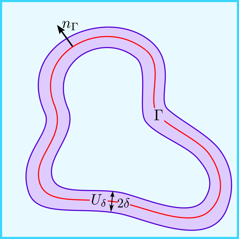
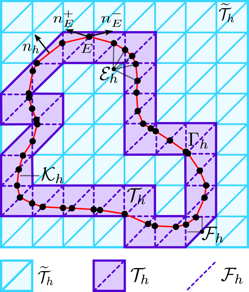
Figure 3.1: Left: The $\delta$ neighborhood of $\Gamma$. Right: Active mesh and discrete surface.

3.2 Discrete weak formulation

To formulate the cut discontinuous Galerkin method for the advection-reaction problem, we need to define averages and jumps of functions across edges and faces. For a piecewise discontinuous, possibly vector-valued function $\sigma$ defined on the surface part $\mathcal{K}_{h}$, we define its average and jump over an edge $E\in\mathcal{E}_{h}$ by

$$\{\sigma\}|_{E} =\frac{1}{2}(\sigma_{E}^{+}+\sigma_{E}^{-}),$$ (3.9)

$$[\sigma]|_{E} =\sigma_{E}^{+}-\sigma_{E}^{-},$$ (3.10)

respectively. To account for the fact that the two co-normals $n_{E}^{\pm}$ are not necessarily co-planar, the normal-weighted average and jump are given by respectively

$$\{\sigma;n_{E}\}|_{E} =\frac{1}{2}(n_{E}^{+}\cdot\sigma^{+}-n_{E}^{-}\cdot\sigma^{-}),$$ (3.11)

$$[\sigma;n_{E}]|_{E} =(n_{E}^{+}\cdot\sigma^{+}+n_{E}^{-}\cdot\sigma^{-}),$$ (3.12)

which reduces to the known standard definitions in the Euclidean case. Similarly, for functions $\mu$ defined on the active background mesh $\mathcal{T}_{h}$, the average and jump over a face $F\in\mathcal{F}_{h}$ are given by

$$\{\mu\}|_{F} =\frac{1}{2}(\mu_{F}^{+}+\mu_{F}^{-}),$$ (3.13)

$$[\mu]|_{F} =\mu_{F}^{+}-\mu_{F}^{-}.$$ (3.14)

We can now formulate the cut discontinuous Galerkin based discretization of the advection-reaction problem (2.8). Let $b_{h}:\Gamma_{h}\rightarrow\mathbb{R}^{d}$, $c_{h}:\Gamma_{h}\rightarrow\mathbb{R}$ and $f_{h}:\Gamma_{h}\rightarrow\mathbb{R}$ be suitably defined representations of $b,c$, and $f$ respectively, defined on the discrete surface $\Gamma_{h}$. Further assumptions for $b_{h},c_{h}$, and $f_{h}$ are given below and specific constructions satisfying these assumptions are presented in Section 4.5. For $v,w\in V_{h}$, the discrete counterpart of $a(\cdot,\cdot)$ is defined by

$$a_{h}(v,w) =(c_{h}v+b_{h}\cdot\nabla_{\Gamma_{h}}v,w)_{\mathcal{K}_{h}}-(\{b_{h};n_{E}\}[v],\{w\})_{\mathcal{E}_{h}}+\frac{1}{2}(|\{b_{h};n_{E}\}|[v],[w])_{\mathcal{E}_{h}}.$$ (3.15)

However, for a “naive” cut discontinuous Galerkin formulation which is solely based on the discrete bilinear (3.15) the following issues need to be addressed. First, as for classical cut finite element formulations of bulk boundary problems [10], small cut elements with neglegible surface part measure $|K|_{d-1}\ll h^{d-1}$ and neglegible edge measure $|E|_{d-2}\ll h^{d-2}$ can lead to severely ill-conditioned system matrices. Second and more importantly, we note that the purely surface-based norms $\|\cdot\|_{\Gamma}$ and $\|b\cdot\nabla_{\Gamma}(\cdot)\|_{\Gamma}$ which are naturally associated with (3.15) do not necessarily define proper norms on $V_{h}$ if the polynomial order $k\geqslant 2$. For instance, the unit sphere can be defined by the level set of the second-order polynomial $\phi(x,y,z)=x^{2}+y^{2}+z^{2}-1\in\mathbb{P}_{\mathrm{dc}}^{2}(\mathcal{T}_{h})$. Neglecting geometric errors and assuming $\Gamma=\Gamma_{h}$ for a moment, we see that in that case both $\|\phi\|_{\Gamma}$ and $\|b\cdot\nabla_{\Gamma}\phi\|_{\Gamma}$ are zero although $\phi\in V_{h}$ is clearly nonvanishing. This issue arises from fact that the aforementioned norms only account for variations of discrete functions in surface tangential direction but not for variations in surface normal direction. As a consequence, it is not possible to establish stability estimates for the bilinear form (5.38) which are not sensitive to the particular cut configuration.

A major contribution of the present work is to show how both issues can be addressed simultaneously by adding a suitably designed stabilization form $s_{h}$. Thanks to $s_{h}$, we gain sufficient control over functions in $V_{h}$ in an enhanced streamline-diffusion type norm $|\mspace{-1.0mu}|\mspace{-1.0mu}|\cdot|\mspace{-1.0mu}|\mspace{-1.0mu}|_{\mathrm{sd},h}$ and are able to derive geometrically robust stability properties and optimal error and condition number estimates all of which are independent of the cut configuration. The stabilization form $s_{h}$ is assumed to be symmetric and positive semi-definite and the final stabilized cut discontinuous Galerkin formulation is to seek $u_{h}\in V_{h}$ such that for all $v_{h}\in V_{h}$

$$A_{h}(u_{h},v)\coloneqq a_{h}(u_{h},v)+s_{h}(u_{h},v)=l(v_{h})\coloneqq(f_{h},v_{h})_{\mathcal{K}_{h}}.$$ (3.16)

The design of a suitable stabilization $s_{h}$ will be the main objective of Section 5.

4 Norms, approximation properties, and inequalities

Before we turn to the derivation of stability and a priori error estimates for the discrete problem (3.16) in the next two sections, we first need to introduce suitable norms and collect several important auxiliary results.

4.1 Norms

First, inspired by the theoretical analysis in [52, 72], we define a characteristic or reference time $\tau_{c}$ via

$$\tau_{c}^{-1}=\|c\|_{0,\infty,\Gamma}+|b|_{1,\infty,\Gamma}+b_{\infty}\kappa,$$ (4.1)

where $b_{\infty}=\|b\|_{0,\infty,\Gamma}$ denotes the reference velocity and $\kappa$ is the maximum principal curvature of $\Gamma$ defined in Section 2. Throughout this work, we assume that the mesh is sufficiently fine in the sense that

$$h\leqslant b_{\infty}\tau_{c}\quad\Leftrightarrow\quad\tau_{c}^{-1}\phi_{b}\leqslant 1,$$ (4.2)

introducing the scaling factor

$$\phi_{b}=h/b_{\infty},$$ (4.3)

which will be omnipresent in the forthcoming stability and error analysis. Assumptions (4.2) ensure that the individual inequalities

$$\|c\|_{0,\infty,\Gamma}h\leqslant b_{\infty},\quad|b|_{1,\infty,\Gamma}\leqslant\dfrac{b_{\infty}}{h},\quad\text{and}\quad h\leqslant\dfrac{1}{\kappa}$$ (4.4)

are all satisfied. The first inequality simply means that on an element level, problem (2.8) can be considered advection-dominant, while the second one ensures that the velocity field $b$ is sufficiently resolved. The third inequality in (4.4) is just a reformulation of our previous assumption that the active mesh lies within an $\delta$-neighborhood $U_{\delta}(\Gamma)$ for which the closest point projection is uniquely defined, cf. Section 3.1.

Next, we define the upwind and the scaled streamline diffusion norm by

$$|\mspace{-1.0mu}|\mspace{-1.0mu}|v|\mspace{-1.0mu}|\mspace{-1.0mu}|_{\mathrm{up}}^{2} =\tau_{c}^{-1}\|v\|_{\mathcal{K}_{h}}^{2}+\frac{1}{2}\||\{b_{h};n_{E}\}|^{\nicefrac{{1}}{{2}}}[v]\|_{\mathcal{E}_{h}}^{2},$$ (4.5)

$$|\mspace{-1.0mu}|\mspace{-1.0mu}|v|\mspace{-1.0mu}|\mspace{-1.0mu}|_{\mathrm{sd}}^{2} =|\mspace{-1.0mu}|\mspace{-1.0mu}|v|\mspace{-1.0mu}|\mspace{-1.0mu}|_{\mathrm{up}}^{2}+\|\phi_{b}^{\nicefrac{{1}}{{2}}}b_{h}\cdot\nabla_{\Gamma_{h}}v\|_{\mathcal{K}_{h}}^{2},$$ (4.6)

On a few occasions, we will also employ a slightly stronger norm than $|\mspace{-1.0mu}|\mspace{-1.0mu}|\cdot|\mspace{-1.0mu}|\mspace{-1.0mu}|_{\mathrm{sd}}$ defined by

$$|\mspace{-1.0mu}|\mspace{-1.0mu}|v|\mspace{-1.0mu}|\mspace{-1.0mu}|_{\mathrm{sd}\ast}^{2}=\phi_{b}^{-1}\|v\|_{\mathcal{K}_{h}}^{2}.+\|\phi_{b}^{\nicefrac{{1}}{{2}}}b_{h}\cdot\nabla_{\Gamma_{h}}v\|_{\mathcal{K}_{h}}^{2}+b_{\infty}\|v\|_{\partial\mathcal{K}_{h}}^{2}$$ (4.7)

as it immediately leads to the following useful boundedness results.

Lemma 4.1

For $v\in H^{1}(\Gamma)\oplus V_{h}$ and $w\in V_{h}$ it holds that

$$a_{h}(v,w)\lesssim|\mspace{-1.0mu}|\mspace{-1.0mu}|v|\mspace{-1.0mu}|\mspace{-1.0mu}|_{\mathrm{sd}\ast}|\mspace{-1.0mu}|\mspace{-1.0mu}|w|\mspace{-1.0mu}|\mspace{-1.0mu}|_{\mathrm{sd}}.$$ (4.8)

The corresponding stabilized norms

$$|\mspace{-1.0mu}|\mspace{-1.0mu}|v|\mspace{-1.0mu}|\mspace{-1.0mu}|_{\bigstar,h}^{2}=|\mspace{-1.0mu}|\mspace{-1.0mu}|v|\mspace{-1.0mu}|\mspace{-1.0mu}|_{\bigstar}^{2}+|v|_{s_{h}}^{2}\quad\text{for }\bigstar\in\{\mathrm{up},\mathrm{sd},\mathrm{sd}\ast\}$$ (4.9)

will play a crucial role in the theoretical analysis of the proposed cut discontinuous Galerkin method. Here, as usual, $|\cdot|_{s_{h}}$ refers to the semi-norm induced by the symmetric stabilization bilinear form $s_{h}$.

4.2 Useful inequalities

In the forthcoming analysis, we will use several inverse inequalities which hold for discrete functions $v_{h}\in V_{h}$, namely

$$\|D^{j}v_{h}\|_{T} \lesssim h^{i-j}\|D^{i}v_{h}\|_{T} \quad\forall\,T\in\mathcal{T}_{h}, \quad 0\leqslant i\leqslant j,$$ (4.10)

$$\|D^{j}v_{h}\|_{\partial T} \lesssim h^{i-j-1/2}\|D^{i}v_{h}\|_{T} \quad\forall\,T\in\mathcal{T}_{h}, \quad 0\leqslant i\leqslant j-1/2,$$ (4.11)

$$\|D^{j}v_{h}\|_{\Gamma\cap T} \lesssim h^{i-j-1/2}\|D^{i}v_{h}\|_{T} \quad\forall\,T\in\mathcal{T}_{h}, \quad 0\leqslant i\leqslant j-1/2,$$ (4.12)

$$\|D^{j}v_{h}\|_{E\cap F} \lesssim h^{i-j-1/2}\|D^{i}v_{h}\|_{F} \quad\forall\,(E,F)\in\mathcal{E}_{h}\times\mathcal{F}_{h}, \quad 0\leqslant i\leqslant j-1/2,$$ (4.13)

while for functions $v\in H^{1}(\mathcal{T}_{h})$ the trace inequalities

$$\|v\|_{\partial T} \lesssim h^{-\nicefrac{{1}}{{2}}}\|v\|_{T}+h^{\nicefrac{{1}}{{2}}}\|\nabla v\|_{T} \quad\forall\,T\in\mathcal{T}_{h},$$ (4.14)

$$\|v\|_{\Gamma\cap T} \lesssim h^{-\nicefrac{{1}}{{2}}}\|v\|_{T}+h^{\nicefrac{{1}}{{2}}}\|\nabla v\|_{T} \quad\forall\,T\in\mathcal{T}_{h},$$ (4.15)

$$\|u\|_{E\cap F} \lesssim h^{-\nicefrac{{1}}{{2}}}\|u\|_{F}+h^{\nicefrac{{1}}{{2}}}\|\nabla u\|_{F} \quad\forall\,(E,F)\in\mathcal{E}_{h}\times\mathcal{F}_{h},$$ (4.16)

will be extremely useful. All the above inequalities are consequences of similar well-known inverse estimates which can be found in, e.g.,  [73, Sec. 4].

4.3 Quasi-interpolation operators

Next, we define two suitable quasi-interpolation operators which will be heavily used throughout the stability and a priori error analysis. First, let $\pi_{h}^{*}:L^{2}(\mathcal{T}_{h})\rightarrow V_{h}$ be the standard $L^{2}$ projection which for $v\in H^{s}(\mathcal{T}_{h})$ and $r\coloneqq\min\{s,k+1\}$ satisfies the error estimates

$$\|v-\pi_{h}^{*}v\|_{k,T}\lesssim h^{r-k}|v|_{r,T} \quad\forall\,T\in\mathcal{T}_{h}, \quad 0\leqslant k\leqslant r,$$ (4.17)

$$\|v-\pi_{h}^{*}v\|_{k,F}\lesssim h^{r-k-1/2}|v|_{r,F} \quad\forall\,F\in\mathcal{F}_{h}, \quad 0\leqslant k\leqslant r-1/2,$$ (4.18)

see [52, Sec. 1.4.4]. Now define $\pi_{h}:H^{s}(\Gamma)\rightarrow V_{h}$ by taking the $L^{2}$-projection of the extension of $v$, so that $\pi_{h}v=\pi_{h}^{*}v^{e}$ for $v\in H^{s}(\Gamma)$. To derive error estimates for this quasi-interpolation operator, we recall the co-area formula

$$\int_{U_{\delta}}f(x)\,\mathrm{d}x=\int_{-\delta}^{\delta}\Big{(}\int_{\Gamma(r)}f(y,r)d\,\Gamma_{r}(y)\Big{)}\,\mathrm{d}r,$$ (4.19)

which can be found for instance in [74, Thm. 3.11]. Thanks to the co-area formula and the assumption $\mathcal{T}_{h}\subset U_{\delta}(\Gamma)$, the extension operator satisfies the estimate

$$\|v^{e}\|_{k,U_{\delta}(\Gamma)}\lesssim\delta^{\nicefrac{{1}}{{2}}}\|v\|_{k,\Gamma},\hskip 14.22636pt0\leqslant k\leqslant s,$$ (4.20)

for $0<\delta<\delta_{0}$, where $\delta\sim h$.

For the forthcoming design and analysis of the stabilization $s_{h}(\cdot,\cdot)$, we need to review some basic facts about the Oswald interpolation operator $\mathcal{O}_{h}:\mathbb{P}_{\mathrm{dc}}^{k}(\mathcal{T}_{h})\rightarrow\mathbb{P}_{\mathrm{c}}^{k}(\mathcal{T}_{h})$, which maps discontinuous piecewise polynomials on $\mathcal{T}_{h}$ to continuous ones. For a function $v_{h}\in\mathbb{P}_{\mathrm{dc}}^{k}(\mathcal{T}_{h})$, its continuous version $\mathcal{O}_{h}(v_{h})$ is defined in each interpolation node $x_{i}$ by taking the average

$$\mathcal{O}_{h}(v_{h})(x_{i})=\frac{1}{\text{card}(\mathcal{T}_{h}(x_{i}))}\sum_{T\in\mathcal{T}_{h}(x_{i})}v_{h}|_{T}(x_{i}),$$ (4.21)

where $\mathcal{T}_{h}(x_{i})$ is the set of all elements $T\in\mathcal{T}_{h}$ sharing the node $x_{i}$. The deviation of $\mathcal{O}_{h}(v_{h})$ from $v_{h}$ can then be measured by the jumps of $v_{h}$ across faces as stated in the following lemma. A proof can be found in [75, Lem. 3.2].

Lemma 4.2

For $v_{h}\in\mathbb{P}_{\mathrm{dc}}^{k}(\mathcal{T}_{h})$ we have

$$\|v_{h}-\mathcal{O}_{h}(v_{h})\|_{T}^{2}\lesssim\sum_{F\in\mathcal{F}_{h}(T)}h\|[v_{h}]\|_{F}^{2},$$ (4.22)

where $\mathcal{F}_{h}(T)$ denotes all faces $F$ in $\mathcal{F}_{h}$ that intersects $T$.

4.4 Domain perturbation related estimates

Using the definition of the discrete surface gradient $\nabla_{\Gamma_{h}}:V_{h}\rightarrow\mathbb{R}^{d}$ and applying the chain rule, we have the well-known identity

$$\nabla_{\Gamma_{h}}u^{e}=B^{T}\nabla_{\Gamma}u,$$ (4.23)

where $B=P_{\Gamma}(I-\rho\mathcal{H})P_{\Gamma_{h}}:T_{x}(K)\rightarrow T_{p(x)}(\Gamma)$, and $\mathcal{H}=\nabla\otimes\nabla\rho$. Note that for $h$ small enough, the linear mapping ${P}_{\Gamma}{P}_{\Gamma_{h}}:T_{x}(K)\rightarrow T_{p(x)}(\Gamma)$ and thus $B={P}_{\Gamma}(I-\rho\mathcal{H}){P}_{\Gamma_{h}}={P}_{\Gamma}{P}_{\Gamma_{h}}+h^{k_{g}+1}$ are invertible as mappings from the discrete to the continuous tangential space, thanks to geometry assumption (3.1). Using (4.23), we can also write the lifting of the gradient from $\Gamma_{h}$ to $\Gamma$ by using

$$\nabla_{\Gamma_{h}}w=\nabla_{\Gamma_{h}}(w^{l})^{e}=B^{T}\nabla_{\Gamma}w^{l},$$ (4.24)

so

$$\nabla_{\Gamma}w^{l}=B^{-T}\nabla_{\Gamma_{h}}w.$$ (4.25)

The measure on $\Gamma$ can be expressed as

$$d\,\Gamma=|B|d\,\Gamma_{h},$$ (4.26)

where $|B|$ is the absolute value of the determinant of $B$. For $B$ and $|B|$ we recall that the assumptions made in (3.1) imply the following estimates

$$\|B\|_{L^{\infty}(\Gamma)}\lesssim 1,\quad\|B^{-1}\|_{L^{\infty}(\Gamma_{h})}\lesssim 1,\quad\|P_{{\Gamma_{h}}}P_{\Gamma}-B^{-1}\|_{L^{\infty}({\Gamma_{h}})}\lesssim h^{k_{g}+1},$$ (4.27)

and

$$\|1-|B|\|_{L^{\infty}({\Gamma_{h}})}\lesssim h^{k_{g}+1},\quad\||B|\|_{L^{\infty}({\Gamma_{h}})}\lesssim 1,\quad\||B^{-1}|\|_{L^{\infty}({\Gamma_{h}})}\lesssim 1,$$ (4.28)

and we refer to for the details. This leads to the norm equivalences

$$\|v^{l}\|_{L^{2}(\Gamma)} \sim\|v\|_{L^{2}(\Gamma_{h})},$$ (4.29)

$$\|\nabla_{\Gamma}v^{l}\|_{L^{2}(\Gamma)} \sim\|\nabla_{\Gamma_{h}}v\|_{L^{2}(\Gamma_{h})}$$ (4.30)

for $v\in H^{1}(\Gamma)^{e}\oplus V_{h}$. Proofs of the above identities, inequalities and norm equivalences can be found in, e.g., [14, 20, 58, 21].

4.5 Assumption on the discrete coefficients

For the discrete coefficient functions $b_{h},c_{h}$ and $f_{h}$, we now formulate several minimal assumptions for the forthcoming stability and error analysis to hold. First, as the expression $b_{h}\cdot\nabla_{\Gamma_{h}}v$ only involves tangential components of $b_{h}$, we simply require that the velocity field $b_{h}$ is purely tangential. Next, we assume that $b_{h}$ and $c_{h}$ admit a discrete version of (2.11),

$$\operatorname*{ess\,inf}_{x\in\Gamma_{h}}\big{(}c_{h}(x)-\frac{1}{2}\nabla_{\Gamma_{h}}\cdot b_{h}(x)\big{)}\geqslant c_{0,h}>0.$$ (4.31)

with some positive and $h$-independent constant $c_{h,0}$. Further, the following approximation properties are supposed to hold,

$$\|P_{\Gamma_{h}}b^{e}-b_{h}\|_{L^{\infty}(\mathcal{K}_{h})}\lesssim C_{b}h^{k_{g}+1},$$ (4.32)

$$\|c^{e}-c_{h}\|_{L^{\infty}(\mathcal{K}_{h})}\lesssim C_{c}h^{k_{g}+1},$$ (4.33)

$$\|f^{e}-f_{h}\|_{L^{\infty}(\mathcal{K}_{h})}\lesssim C_{f}h^{k_{g}+1}.$$ (4.34)

In addition to the $k_{g}+1$ order estimate (4.32), we also assume a first-order estimate of the form

$$\|P_{\Gamma_{h}}b^{e}-b_{h}\|_{L^{\infty}(\mathcal{K}_{h})} \lesssim h(b_{\infty}\kappa+|b|_{1,\infty,\Gamma}),$$ (4.35)

which we will see is sufficient to ensure that stabilized CutDG formulation (3.16) satisfies a discrete inf-sup condition. Finally, we also assume the existence of a piecewise constant vector field ${\widetilde{b}}_{h}$ satisfying

$$\|P_{\Gamma_{h}}b^{e}-{\widetilde{b}}_{h}\|_{L^{\infty}(\mathcal{K}_{h})} \lesssim h(b_{\infty}\kappa+|b|_{1,\infty,\Gamma})$$ (4.36)

$$\|b^{e}-{\widetilde{b}}_{h}\|_{0,\infty,T} \lesssim h(b_{\infty}\kappa+|b|_{1,\infty,\Gamma}),\quad\|{\widetilde{b}}_{h}\|_{0,\infty,T}\lesssim\|b\|_{0,\infty,\Gamma}.$$ (4.37)

Since the extended vector field $b^{e}$ is in $W^{1,\infty}(U_{\delta}(\Gamma))$, such a patch-wise defined, locally constant, vector field $\widetilde{b}_{h}$ satisfying the assumptions above can always be constructed, by for example taking the value of $b_{h}$ at a point in the patch.

Thanks to the domain-perturbation-related estimates reviewed in the previous section, the approximation properties can be reformulated in a manner that will be more convenient in the analysis of the geometrical errors presented in Section 6.3.

Lemma 4.3

Assume that $b_{h},c_{h}$, and $f_{h}$ satisfy (4.32)–(4.34), then it holds that

$$\||B|B^{-1}b^{e}-b_{h}\|_{L^{\infty}(\mathcal{K}_{h})} \lesssim C_{b}h^{k_{g}+1},$$ (4.38)

$$\||B|c^{e}-c_{h}\|_{L^{\infty}(\mathcal{K}_{h})} \lesssim C_{c}h^{k_{g}+1},$$ (4.39)

$$\||B|f^{e}-f_{h}\|_{L^{\infty}(\mathcal{K}_{h})} \lesssim C_{f}h^{k_{g}+1}.$$ (4.40)

Proof 1

The proof in [37, Sec. 4.2] for $k_{g}=1$ immediately generalizes to our geometrical assumptions, but for the reader’s convenience, we provide a short proof in A.

We conclude this section by recalling an estimate for the co-normal jump of the discrete velocity $b_{h}$ which will come in handy when turning to the stability and a priori error analysis of the proposed CutDG method.

Lemma 4.4

Assume that the geometric approximation assumption (3.1) holds and that $b_{h}$ satisfies (4.32). Then

$$\|[b_{h};n_{E}]\|_{L^{\infty}(\mathcal{E}_{h})} \lesssim C_{b}h^{k_{g}+1}.$$ (4.41)

Proof 2

A proof for the case $d=2$ and $k_{g}=1$ can be found in, e.g., [34, Lemma 3.6]. For the reader’s convenience, a slightly generalized proof for $d\geqslant 2$ and $k_{g}\geqslant 1$ is given in A.

5 Stability analysis

A key observation made at the end of Section 3.2 is that the purely surface-based bilinear form $a_{h}$ and its associated “norm” $|\mspace{-1.0mu}|\mspace{-1.0mu}|\cdot|\mspace{-1.0mu}|\mspace{-1.0mu}|_{\mathrm{sd}}$ do not provide sufficient control over a discrete function $v_{h}\in V_{h}$ defined on the active mesh $\mathcal{T}_{h}$. The major objective of this section is to show that if we augment $a_{h}$ by a suitably constructed stabilization form $s_{h}$, control over $V_{h}$ in the resulting enhanced norm $|\mspace{-1.0mu}|\mspace{-1.0mu}|\cdot|\mspace{-1.0mu}|\mspace{-1.0mu}|_{\mathrm{sd},h}$ is regained which allows us to prove a geometrically robust inf-sup condition with respect to the $|\mspace{-1.0mu}|\mspace{-1.0mu}|\cdot|\mspace{-1.0mu}|\mspace{-1.0mu}|_{\mathrm{sd},h}$ norm.

5.1 Construction of the stabilization form $s_{h}$

As the model problem (2.8) consists of an advection-reaction operator, it is natural to assume that a suitably designed stabilization will acknowledge this. We thus start by considering the norm part which is typically associated with the reaction term. Here, it is more natural to use the rescaled or extended $L^{2}$ norm $(\tau_{c}h)^{-\nicefrac{{1}}{{2}}}\|v_{h}\|_{\mathcal{T}_{h}}$ instead of the purely surface-based norm $\tau_{c}^{-\nicefrac{{1}}{{2}}}\|\cdot\|_{\Gamma_{h}}$ since the former provides a proper norm for discrete functions defined on the active mesh $\mathcal{T}_{h}$. The following lemma (first proved in [21, 20]) then shows that for a continuous, discrete function $v_{h}\in\mathbb{P}_{\mathrm{c}}^{k}(\mathcal{T}_{h})$, the extended $L^{2}$ norm can be bounded by the surface $L^{2}$ norm if enhanced by the volume-based normal gradient stabilization, which provides sufficient control in normal directions.

Lemma 5.1

For $v\in\mathbb{P}_{\mathrm{c}}^{k}(\mathcal{T}_{h})$ it holds that

$$h^{-1}\|v\|_{\mathcal{T}_{h}}^{2} \lesssim\|v\|_{\mathcal{K}_{h}}^{2}+h\|n_{\Gamma_{h}}\cdot\nabla v\|_{\mathcal{T}_{h}}^{2}.$$ (5.1)

Our first task is to extend the previous lemma to discontinuous element-wise polynomials.

Lemma 5.2

For $v\in\mathbb{P}_{\mathrm{dc}}^{k}(\mathcal{T}_{h})$ it holds that

$$h^{-1}\|v\|_{\mathcal{T}_{h}}^{2} \lesssim\|v\|_{\mathcal{K}_{h}}^{2}+\|[v]\|_{\mathcal{F}_{h}}^{2}+h\|n_{\Gamma_{h}}\cdot\nabla v\|_{\mathcal{T}_{h}}^{2}.$$ (5.2)

Proof 3

We use the Oswald interpolant $\mathcal{O}_{h}$ reviewed in Section 4.3 to create a continuous version of $v$ which is eligible for an application of Lemma 5.1. Set $\widetilde{v}=\mathcal{O}_{h}(v)\in\mathbb{P}_{\mathrm{c}}^{k}(\mathcal{T}_{h})$. Using Lemma 5.1 in combination with the inverse estimates (4.10),(4.12), and Lemma (4.2) on the Oswald interpolant results in the following chain of estimates:

$$\|v\|_{\mathcal{T}_{h}}^{2} \lesssim\|\widetilde{v}\|_{\mathcal{T}_{h}}^{2}+\|v-\widetilde{v}\|_{\mathcal{T}_{h}}^{2}$$ (5.3)

$$\lesssim h\|\widetilde{v}\|_{\mathcal{K}_{h}}^{2}+h^{2}\|n_{\Gamma_{h}}\cdot\nabla\widetilde{v}\|_{\mathcal{T}_{h}}^{2}+\|v-\widetilde{v}\|_{\mathcal{T}_{h}}^{2}$$ (5.4)

$$\lesssim h\|v\|_{\mathcal{K}_{h}}^{2}+h\|\widetilde{v}-v\|_{\mathcal{K}_{h}}^{2}+h^{2}\|n_{\Gamma_{h}}\cdot\nabla v\|_{\mathcal{T}_{h}}^{2}+h^{2}\|n_{\Gamma_{h}}\cdot\nabla(\widetilde{v}-v)\|_{\mathcal{T}_{h}}^{2}+\|v-\widetilde{v}\|_{\mathcal{T}_{h}}^{2}$$ (5.5)

$$\lesssim h\|v\|_{\mathcal{K}_{h}}^{2}+\|\widetilde{v}-v\|_{\mathcal{T}_{h}}^{2}+h^{2}\|n_{\Gamma_{h}}\cdot\nabla v\|_{\mathcal{T}_{h}}^{2}+\|\widetilde{v}-v\|_{\mathcal{T}_{h}}^{2}+\|v-\widetilde{v}\|_{\mathcal{T}_{h}}^{2}$$ (5.6)

$$\lesssim h\|v\|_{\mathcal{K}_{h}}^{2}+h^{2}\|n_{\Gamma_{h}}\cdot\nabla v\|_{\mathcal{T}_{h}}^{2}+\|v-\widetilde{v}\|_{\mathcal{T}_{h}}^{2}$$ (5.7)

$$\lesssim h\|v\|_{\mathcal{K}_{h}}^{2}+h^{2}\|n_{\Gamma_{h}}\cdot\nabla v\|_{\mathcal{T}_{h}}^{2}+h\|[v]\|_{\mathcal{F}_{h}}^{2}.$$ (5.8)

The previous lemma motivates the following definition of a reaction-term associated stabilization $s_{h}^{c}$ of the form

$$s_{h}^{c}(v,w)\coloneqq\gamma^{c}_{0}\tau_{c}^{-1}([v],[w])_{\mathcal{F}_{h}}+\gamma^{c}_{n}\tau_{c}^{-1}h(n_{\Gamma_{h}}\cdot\nabla v,n_{\Gamma_{h}}\cdot\nabla w)_{\mathcal{T}_{h}}\quad\text{for }v,w\in V_{h},$$ (5.9)

with $\gamma_{0}^{c}$ and $\gamma_{n}^{c}$ being dimensionless, positive stability parameters. Thanks to Lemma 5.2, incorporating $s_{h}^{c}$ into $s_{h}$ gives us control over the extended $L^{2}$ norm in the sense that

$$(\tau_{c}h)^{-1}\|v\|_{\mathcal{T}_{h}}^{2}\lesssim|\mspace{-1.0mu}|\mspace{-1.0mu}|v|\mspace{-1.0mu}|\mspace{-1.0mu}|_{\mathrm{up},h}^{2}$$ (5.10)

holds for $v\in V_{h}$. We refer to (5.10) by saying that $s_{h}^{c}$ satisfies an $L^{2}$-norm extension property.

We turn to the stabilization of the $|\mspace{-1.0mu}|\mspace{-1.0mu}|\cdot|\mspace{-1.0mu}|\mspace{-1.0mu}|_{\mathrm{sd}}$ norm. As in the analysis of the classical upwind stabilized DG method [46, 52], we will exploit that the scaled streamline derivative $\phi_{b}b_{h}\cdot\nabla_{\Gamma_{h}}v_{h}=\phi_{b}b_{h}\cdot\nabla v_{h}$ is (almost) a valid test function if only $b_{h}$ is replaced by an element-wise constant, $\widetilde{b}_{h}$, which satisfies (4.36). Moreover, similar to ${\widetilde{b}}_{h}$ we can construct an element-wise constant approximation, $\widetilde{n}_{\Gamma_{h}}$, of $n_{\Gamma_{h}}$ which satisfies the estimate

$$\|n_{\Gamma_{h}}-\widetilde{n}_{\Gamma_{h}}\|_{\infty}\lesssim\kappa h.$$ (5.11)

The next lemma will help us to quantify the errors introduced when switching between $b_{h}$ and $\widetilde{b}_{h}$ respectively $n_{{\Gamma_{h}}}$ and $\widetilde{n}_{{\Gamma_{h}}}$ in the forthcoming stability analysis.

Lemma 5.3

For $v\in V_{h}$, it holds that

$$\bigl{(}b_{\infty}\|\widetilde{n}_{{\Gamma_{h}}}-n_{{\Gamma_{h}}}\|_{0,\infty,\mathcal{T}_{h}}^{2}+\dfrac{\phi_{b}}{h}\|\widetilde{b}_{h}-b_{h}\|_{0,\infty,\mathcal{T}_{h}}^{2}\bigr{)}\|\nabla v\|_{\mathcal{T}_{h}}^{2}\lesssim(\tau_{c}h)^{-1}\|v\|_{\mathcal{T}_{h}}^{2}\lesssim|\mspace{-1.0mu}|\mspace{-1.0mu}|v|\mspace{-1.0mu}|\mspace{-1.0mu}|_{\mathrm{up},h}^{2}.$$ (5.12)

Proof 4

First, simply using inverse estimate (4.10) together with (5.11) shows that

$$b_{\infty}\|\widetilde{n}_{{\Gamma_{h}}}-n_{{\Gamma_{h}}}\|_{0,\infty,\mathcal{T}_{h}}^{2}\|\nabla v\|_{\mathcal{T}_{h}}^{2} \lesssim(b_{\infty}\kappa)(\kappa h)h^{-1}\|v\|_{\mathcal{T}_{h}}^{2}\lesssim(\tau_{c}h)^{-1}\|v\|_{\mathcal{T}_{h}}^{2}$$ (5.13)

since $b_{\infty}\kappa\leqslant\tau_{c}^{-1}$ by the definition of $\tau_{c}$ (4.1) and $\kappa h\lesssim 1$ (4.4). Next, by (4.1) and assumption (4.2) $(|b|_{1,\infty,\Gamma}+b_{\infty}\kappa)\phi_{b}\leqslant\tau_{c}^{-1}\phi_{b}\lesssim 1$ holds and therefore adding and subtracting ${P}_{\Gamma_{h}}b$ in the second term in the left-hand side of (5.12) together with (4.35), (4.36), and (4.10) yields

$$\dfrac{\phi_{b}}{h}\|{\widetilde{b}}_{h}-b_{h}\|_{0,\infty,\mathcal{T}_{h}}^{2}\|\nabla v\|_{\mathcal{T}_{h}}^{2}\lesssim\dfrac{\phi_{b}}{h}(|b|_{1,\infty,T}+b_{\infty}\kappa)^{2}\|v\|_{\mathcal{T}_{h}}^{2}\lesssim(\tau_{c}h)^{-1}\|v\|_{\mathcal{T}_{h}}^{2}.$$ (5.14)

Collecting the bounds (5.13) and (5.14) proves the first inequality in (5.12) while the second follows immediately from $L^{2}$-norm extension property (5.10).

With these preparations at hand, we can now show that —similar to the extended $L^{2}$-norm— the extended streamline diffusion norm can be controlled by the surface streamline diffusion norm if suitable stabilization terms are added:

Lemma 5.4

Let ${\widetilde{b}}_{h}$ be an element-wise constant vector field satisfying (4.36). For $v\in\mathbb{P}_{\mathrm{dc}}^{k}(\mathcal{T}_{h})$ we have the estimate

$$\frac{1}{h}\|\phi_{b}^{\nicefrac{{1}}{{2}}}\widetilde{b}_{h}\cdot\nabla v\|_{\mathcal{T}_{h}}^{2}\lesssim \|\phi_{b}^{\nicefrac{{1}}{{2}}}b_{h}\cdot\nabla_{\Gamma_{h}}v\|_{\mathcal{K}_{h}}^{2}+\frac{b_{\infty}}{h}\|[v]\|_{\mathcal{F}_{h}}^{2}+b_{\infty}h\|[n_{F}\cdot\nabla v]\|_{\mathcal{F}_{h}}^{2}$$

$$\quad+b_{\infty}\|n_{\Gamma_{h}}\cdot\nabla v\|_{\mathcal{T}_{h}}^{2}+|\mspace{-1.0mu}|\mspace{-1.0mu}|v|\mspace{-1.0mu}|\mspace{-1.0mu}|_{\mathrm{up},h}^{2}.$$ (5.15)

Proof 5

We start by applying Lemma 5.2 to the discrete function $\phi_{b}^{\nicefrac{{1}}{{2}}}\widetilde{b}_{h}\cdot\nabla v\in V_{h}$, yielding

$$\frac{1}{h}\|\phi_{b}^{\nicefrac{{1}}{{2}}}\widetilde{b}_{h}\cdot\nabla v\|_{\mathcal{T}_{h}}^{2} \lesssim\|\phi_{b}^{\nicefrac{{1}}{{2}}}\widetilde{b}_{h}\cdot\nabla v\|_{\mathcal{K}_{h}}^{2}+\|[\phi_{b}^{\nicefrac{{1}}{{2}}}\widetilde{b}_{h}\cdot\nabla v]\|_{\mathcal{F}_{h}}^{2}+h\|n_{\Gamma_{h}}\cdot\nabla(\phi_{b}^{\nicefrac{{1}}{{2}}}\widetilde{b}_{h}\cdot\nabla v)\|_{\mathcal{T}_{h}}^{2}$$

$$=I+II+III.$$ (5.16)

Recalling (5.12) and the inverse estimate (4.12), we see that term $I$ can be bounded by

$$I\lesssim\|\phi_{b}^{\nicefrac{{1}}{{2}}}b_{h}\cdot\nabla_{\Gamma_{h}}v\|_{\mathcal{K}_{h}}^{2}+\dfrac{1}{h}\|\phi_{b}^{\nicefrac{{1}}{{2}}}(\widetilde{b}_{h}-b_{h})\cdot\nabla v\|_{\mathcal{T}_{h}}^{2}\lesssim\|\phi_{b}^{\nicefrac{{1}}{{2}}}b_{h}\cdot\nabla_{\Gamma_{h}}v\|_{\mathcal{K}_{h}}^{2}+(\tau_{c}h)^{-1}\|v\|_{\mathcal{T}_{h}}^{2}$$ (5.17)

Next, to estimate term $II$, we can switch between ${\widetilde{b}}_{h}$ and $b^{e}$ and control the difference term again by the $|\mspace{-1.0mu}|\mspace{-1.0mu}|\cdot|\mspace{-1.0mu}|\mspace{-1.0mu}|_{\mathrm{up},h}$ norm. Using the fact that $[b^{e}]=0$, we obtain

$$II \lesssim b_{\infty}h\|[\nabla v]\|_{\mathcal{F}_{h}}^{2}+\|[\phi_{b}^{\nicefrac{{1}}{{2}}}(b^{e}-\widetilde{b}_{h})\cdot\nabla v]\|_{\mathcal{F}_{h}}^{2}=II_{a}+II_{b}.$$ (5.18)

Now let $P_{F}\nabla v$ be the part of $\nabla v$ that is tangential to $F$, so that $\nabla v=P_{F}\nabla v+(n_{F}\cdot\nabla v)n_{F}$. Applying an inverse estimate similar to (4.10) to $\|P_{F}\nabla v\|_{F}$ allows us to bound $II_{a}$ by

$$II_{a} =hb_{\infty}\|[P_{F}\nabla v]\|_{\mathcal{F}_{h}}^{2}+hb_{\infty}\|[n_{F}\cdot\nabla v]\|_{\mathcal{F}_{h}}^{2}\lesssim\frac{b_{\infty}}{h}\|[v]\|_{\mathcal{F}_{h}}^{2}+hb_{\infty}\|[n_{F}\cdot\nabla v]\|_{\mathcal{F}_{h}}^{2}.$$ (5.19)

For the second contribution $II_{b}$, we first recall the assumptions (4.37) which together with the inverse estimate (4.11) yields

$$II_{b}\lesssim\frac{\phi_{b}}{h}(b_{\infty}\kappa+|b|_{1,\infty,\Gamma})^{2}\|v\|^{2}_{\mathcal{T}_{h}}\lesssim\frac{\phi_{b}}{h}\tau_{c}^{-2}\lesssim(\tau_{c}h)^{-1}\|v\|_{\mathcal{T}_{h}}^{2}.$$ (5.20)

where in the last step we again used that $\tau_{c}^{-1}\phi_{b}\lesssim 1$ by our assumption 4.2 on the mesh resolution.

Finally, we turn to the remaining term $III$ in (5.16). Similar to ${\widetilde{b}}_{h}$, let $\widetilde{n}_{\Gamma_{h}}$ be an element-wise constant approximation of $n_{\Gamma_{h}}$ such that $\|n_{\Gamma_{h}}-\widetilde{n}_{\Gamma_{h}}\|_{\infty}\lesssim\kappa h$. Then $\widetilde{n}_{\Gamma_{h}}\cdot\nabla(\widetilde{b}_{h}\cdot\nabla v)=\widetilde{b}_{h}\cdot\nabla(\widetilde{n}_{\Gamma_{h}}\cdot\nabla v)$ and thus in combination with multiple applications of the inverse estimate (4.10) we derive that

$$III =h\|n_{\Gamma_{h}}\cdot\nabla(\phi_{b}^{\nicefrac{{1}}{{2}}}\widetilde{b}_{h}\cdot\nabla v)\|_{\mathcal{T}_{h}}^{2}$$ (5.21)

$$\lesssim h\phi_{b}\|\widetilde{n}_{\Gamma_{h}}\cdot\nabla(\widetilde{b}_{h}\cdot\nabla v)\|_{\mathcal{T}_{h}}^{2}+h\phi_{b}\|(n_{\Gamma_{h}}-\widetilde{n}_{\Gamma_{h}})\cdot\nabla(\widetilde{b}_{h}\cdot\nabla v)\|_{\mathcal{T}_{h}}^{2}$$ (5.22)

$$\lesssim h\phi_{b}\|\widetilde{b}_{h}\cdot\nabla(\widetilde{n}_{\Gamma_{h}}\cdot\nabla v)\|_{\mathcal{T}_{h}}^{2}+\phi_{b}\kappa^{2}h^{3}\|\nabla(\widetilde{b}_{h}\cdot\nabla v)\|_{\mathcal{T}_{h}}^{2}$$ (5.23)

$$\lesssim h^{-1}\phi_{b}b_{\infty}^{2}\|\widetilde{n}_{\Gamma_{h}}\cdot\nabla v\|_{\mathcal{T}_{h}}^{2}+\phi_{b}\kappa^{2}b_{\infty}^{2}h\|\nabla v\|_{\mathcal{T}_{h}}^{2}$$ (5.24)

$$\lesssim b_{\infty}\|\widetilde{n}_{\Gamma_{h}}\cdot\nabla v\|_{\mathcal{T}_{h}}^{2}+(\tau_{c}h)^{-1}\|v\|_{\mathcal{T}_{h}}^{2}$$ (5.25)

$$\lesssim b_{\infty}\|n_{\Gamma_{h}}\cdot\nabla v\|_{\mathcal{T}_{h}}^{2}+b_{\infty}\|(n_{\Gamma_{h}}-\widetilde{n}_{\Gamma_{h}})\cdot\nabla v\|_{\mathcal{T}_{h}}^{2}+(\tau_{c}h)^{-1}\|v\|_{\mathcal{T}_{h}}^{2}$$ (5.26)

$$\lesssim b_{\infty}\|n_{\Gamma_{h}}\cdot\nabla v\|_{\mathcal{T}_{h}}^{2}+(\tau_{c}h)^{-1}\|v\|_{\mathcal{T}_{h}}^{2}.$$ (5.27)

Here, we used the fact that thanks to assumption (4.2), $\phi_{b}\kappa^{2}b_{\infty}^{2}\lesssim\tau_{c}^{-1}$ to pass to (5.25), and in the last step, Lemma 5.3 was employed. Finally, collecting the obtained bounds (5.17), (5.19), (5.20), and (5.27) and applying Lemma 5.12 once more to bound $(\tau_{c}h)^{-1}\|v\|_{\mathcal{T}_{h}}^{2}$ by $|\mspace{-1.0mu}|\mspace{-1.0mu}|v|\mspace{-1.0mu}|\mspace{-1.0mu}|_{\mathrm{up},h}^{2}$ yields the desired estimate.

Motivated by Lemma 5.4, we define now our stabilization for the advection part and set

$$s_{h}^{a}(v,w)=\frac{\gamma^{b}_{0}b_{\infty}}{h}([v],[w])_{\mathcal{F}_{h}}+\gamma^{b}_{1}hb_{\infty}([n_{F}\cdot\nabla v],[n_{F}\cdot\nabla w])_{\mathcal{F}_{h}}+\gamma^{b}_{n}b_{\infty}(n_{\Gamma_{h}}\cdot\nabla v,n_{\Gamma_{h}}\cdot\nabla w)_{\mathcal{T}_{h}}.$$ (5.28)

Thus, combining the reaction- and advection-related stabilization forms suggest considering

$$s_{h}(v,w) =(\gamma^{c}_{0}\tau_{c}^{-1}+\dfrac{\gamma^{b}_{0}b_{\infty}}{h})([v],[w])_{\mathcal{F}_{h}}+\gamma^{b}_{1}b_{\infty}h([n_{F}\cdot\nabla v],[n_{F}\cdot\nabla w])_{\mathcal{F}_{h}}$$

$$\quad+(\gamma^{c}_{n}\tau_{c}^{-1}h+\gamma^{b}_{n}b_{\infty})(n_{\Gamma_{h}}\cdot\nabla v,n_{\Gamma_{h}}\cdot\nabla w)_{\mathcal{T}_{h}}$$ (5.29)

as a candidate for the total stabilization form. However, thanks to Assumption (4.2), we only need to consider the advection part since $\tau_{c}^{-1}\leqslant\phi_{b}^{-1}=\tfrac{b_{\infty}}{h}$, leading us to the final definition of $s_{h}$.

Definition 5.5 (Stabilization form $s_{h}$)

The stabilization $s_{h}$ is given by

$$s_{h}(v,w) =\dfrac{\gamma_{0}b_{\infty}}{h}([v],[w])_{\mathcal{F}_{h}}+\gamma_{1}b_{\infty}h([n_{F}\cdot\nabla v],[n_{F}\cdot\nabla w])_{\mathcal{F}_{h}}+\gamma_{n}b_{\infty}(n_{\Gamma_{h}}\cdot\nabla v,n_{\Gamma_{h}}\cdot\nabla w)_{\mathcal{T}_{h}}$$ (5.30)

with $\gamma_{0},\gamma_{1}$, and $\gamma_{n}$ being dimensionless, positive stability parameters which depend on $k,d$, the quasi-uniformity of $\mathcal{T}_{h}$, and the curvature of $\Gamma$.

For future reference, we summarize our discussion in the following corollary.

Corollary 5.6

Both the extended $L^{2}$ and streamline diffusion norm can be controlled by augmenting the standard streamline diffusion norm (4.6) with the semi-norm $|\cdot|_{s_{h}}$ induced by (5.30) in the sense that

$$\frac{1}{h}\|\phi_{b}^{\nicefrac{{1}}{{2}}}\widetilde{b}_{h}\cdot\nabla v\|_{\mathcal{T}_{h}}^{2}+\frac{1}{h}\|\tau_{c}^{-\nicefrac{{1}}{{2}}}v\|_{\mathcal{T}_{h}}^{2}\lesssim|\mspace{-1.0mu}|\mspace{-1.0mu}|v|\mspace{-1.0mu}|\mspace{-1.0mu}|_{\mathrm{sd},h}^{2}$$ (5.31)

holds for $v\in V_{h}$.

5.2 $\mathbf{L^{2}}$-coercivity for $A_{h}$

Next, we wish to show that the bilinear form $A_{h}$ is coercive with respect to the $|\mspace{-1.0mu}|\mspace{-1.0mu}|\cdot|\mspace{-1.0mu}|\mspace{-1.0mu}|_{\mathrm{up},h}$ norm. As usual, the approach is based on exploiting the skew-symmetry of the advection-related terms via an integration by parts argument, but in contrast to the classical Euclidean case, an additional term arises from the fact that the co-normal vectors $n_{E}+$ and $n_{E}^{-}$ are not co-planar. More precisely, for the co-normal jump, the following result holds.

Lemma 5.7

Given a vector field $b$ and scalar fields $v$ and $w$ for which we assume the edge jump and average to be well-defined. Then

$$[vb;n_{E}]=[v]\{b;n_{E}\}+\{v\}[b;n_{E}]$$ (5.32)

and

$$[bvw;n_{E}]=\{b;n_{E}\}[v]\{w\}+\{b;n_{E}\}\{v\}[w]+[b;n_{E}]\{vw\}.$$ (5.33)

Proof 6

Writing out the definition of surface jumps and averages shows that

$$[v]\{b;n_{E}\}+\{v\}[b;n_{E}] =(v^{+}-v^{-})\frac{1}{2}(n_{E}^{+}b^{+}-n_{E}^{-}b^{-})+\frac{1}{2}(v^{+}+v^{-})(n_{E}^{+}b^{+}+n_{E}^{-}b^{-})$$ (5.34)

$$=\frac{1}{2}(v^{+}n_{E}^{+}b^{+}-v^{+}n_{E}^{-}b^{-}-v^{-}n_{E}^{+}b^{+}+v^{-}n_{E}^{-}b^{-}$$ (5.35)

$$\hskip 14.22636pt+v^{+}n_{E}^{+}b^{+}+v^{+}n_{E}^{-}b^{-}+v^{-}n_{E}^{+}b^{+}+v^{-}n_{E}^{-}b^{-})$$

$$=v^{+}n_{E}^{+}b^{+}+v^{-}n_{E}^{-}b^{-}=[vb;n_{E}].$$ (5.36)

Inserting $vw$ for $v$ in the above argument and applying the standard equality for jumps and averages, $[vw]=\{v\}[w]+[v]\{w\}$, yields equation (5.33).

Using Lemma 5.7 and integrating $(b_{h}\cdot\nabla_{\Gamma_{h}}v,w)$ by parts, we see that

$$(b_{h}\cdot\nabla_{\Gamma_{h}}v,w)_{\mathcal{K}_{h}} =-(v,b_{h}\cdot\nabla_{\Gamma_{h}}w)_{\mathcal{K}_{h}}-(\nabla_{\Gamma_{h}}\cdot b_{h}v,w)_{\mathcal{K}_{h}}+\int_{\mathcal{E}_{h}}[b_{h}vw;n_{E}]\mathrm{d}\mathcal{E}_{h}$$

$$=-(v,b_{h}\cdot\nabla_{\Gamma_{h}}w)_{\mathcal{K}_{h}}-(v,\nabla_{\Gamma_{h}}\cdot b_{h}w)_{\mathcal{K}_{h}}$$ (5.37)

$$\quad+(\{b_{h};n_{E}\}[v],\{w\})_{\mathcal{E}_{h}}+(\{b_{h};n_{E}\}\{v\},[w])_{\mathcal{E}_{h}}$$

$$\quad+(\{vw\},[b_{h};n_{E}])_{\mathcal{E}_{h}}.$$

If we insert (5.37) into (3.15), we see that $a_{h}(\cdot,\cdot)$ is equivalent to

$$a_{h}(v,w) =(c_{h}v,w)_{\mathcal{K}_{h}}+(b_{h}\cdot\nabla_{\Gamma_{h}}v,w)_{\mathcal{K}_{h}}-(\{b_{h};n_{E}\}[v],\{w\})_{\mathcal{E}_{h}}+\frac{1}{2}(|\{b_{h};n_{E}\}|[v],[w])_{\mathcal{E}_{h}}$$ (5.38)

$$=(v,(c_{h}-\nabla_{\Gamma_{h}}\cdot b_{h})w)_{\mathcal{K}_{h}}-(v,b_{h}\cdot\nabla_{\Gamma_{h}}w)_{\mathcal{K}_{h}}+(\{b_{h};n_{E}\}\{v\},[w])_{\mathcal{E}_{h}}$$ (5.39)

$$\quad+\frac{1}{2}(|\{b_{h};n_{E}\}|[v],[w])_{\mathcal{E}_{h}}+(\{vw\},[b_{h};n_{E}])_{\mathcal{E}_{h}}.$$

Thus, by combining one half of both (5.38) and (5.39), the bilinear form $a_{h}(\cdot,\cdot)$ can be divided into a symmetric and a skew-symmetric part,

$$a_{h}(v,w) =a_{h}^{\mathrm{sy}}(v,w)+a_{h}^{\mathrm{sk}}(v,w),$$ (5.40)

where

$$a_{h}^{\mathrm{sy}}(v,w) =((c_{h}-\frac{1}{2}\nabla_{\Gamma_{h}}\cdot b_{h})v,w)_{\mathcal{K}_{h}}+\frac{1}{2}(|\{b_{h};n_{E}\}|[v],[w])_{\mathcal{E}_{h}}+\dfrac{1}{2}(\{vw\},[b_{h};n_{E}])_{\mathcal{E}_{h}},$$ (5.41)

$$a_{h}^{\mathrm{sk}}(v,w) =\frac{1}{2}(b_{h}\cdot\nabla_{\Gamma_{h}}v,w)_{\mathcal{K}_{h}}-\frac{1}{2}(v,b_{h}\cdot\nabla_{\Gamma_{h}}w)_{\mathcal{K}_{h}}$$ (5.42)

$$\quad-\frac{1}{2}(\{b_{h};n_{E}\}[v],\{w\})_{\mathcal{E}_{h}}+\frac{1}{2}(\{b_{h};n_{E}\}\{v\},[w])_{\mathcal{E}_{h}}.$$

Note that even with the standard assumption (4.31), it is not obvious that the symmetric part is positive definite due to the last term in (5.41) arising from the lack of co-planarity of the edge normal vectors. Nevertheless, the next lemma shows that thanks to the stabilization term $s_{h}$, the symmetric part $a_{h}^{\mathrm{sy}}$ is in fact $L^{2}$ coercive.

Lemma 5.8

If the geometry assumption (3.1) and assumption (4.31) on the coefficients $c_{h}$ and $b_{h}$ hold, the stabilized bilinear form $A_{h}=a_{h}+s_{h}$ is coercive with respect to the stabilized upwind norm; that is,

$$A_{h}(v,v)\gtrsim c_{0}\tau_{c}|\mspace{-1.0mu}|\mspace{-1.0mu}|v|\mspace{-1.0mu}|\mspace{-1.0mu}|_{\mathrm{up},h}^{2}\quad\forall\,v\in V_{h}.$$ (5.43)

Proof 7

From decomposing $a_{h}$ into its symmetric and skew-symmetric part, cf. (5.40), it follows that

$$A_{h}(v,v) =((c_{h}-\frac{1}{2}\nabla_{\Gamma_{h}}\cdot b_{h})v,v)_{\mathcal{K}_{h}}+\frac{1}{2}(|\{b_{h};n_{E}\}|[v],[v])_{\mathcal{E}_{h}}+(\{v^{2}\},[b_{h};n_{E}])_{\mathcal{E}_{h}}+s_{h}(v,v)$$ (5.44)

$$\geqslant c_{0,h}(v,v)_{\mathcal{K}_{h}}+\frac{1}{2}(|\{b_{h};n_{E}\}|[v],[v])_{\mathcal{E}_{h}}+s_{h}(v,v)+(\{v^{2}\},[b_{h};n_{E}])_{\mathcal{E}_{h}}.$$ (5.45)

$$\gtrsim c_{0,h}\tau_{c}|\mspace{-1.0mu}|\mspace{-1.0mu}|v|\mspace{-1.0mu}|\mspace{-1.0mu}|_{\mathrm{up},h}^{2}+(\{v^{2}\},[b_{h};n_{E}])_{\mathcal{E}_{h}}.$$ (5.46)

The remaining $(\{v^{2}\},[b_{h};n_{E}])_{\mathcal{E}_{h}}$ term in (5.46) can be handled by combining the inverse estimates (4.13) and (4.11) with (5.10) leading to

$$(\{v^{2}\},[b_{h};n_{E}])_{\mathcal{E}_{h}} \lesssim h^{-2}\|v\|_{\mathcal{T}_{h}}^{2}C_{b}h^{k_{g}+1}=(h\tau_{c})^{-1}\|v\|_{\mathcal{T}_{h}}^{2}\tau_{c}C_{b}h^{k_{g}}\lesssim|\mspace{-1.0mu}|\mspace{-1.0mu}|v|\mspace{-1.0mu}|\mspace{-1.0mu}|_{\mathrm{up},h}\tau_{c}c_{0,h}\dfrac{C_{b}h^{k_{g}}}{c_{0,h}}.$$ (5.47)

Inserting this into (5.46) we see that

$$A_{h}(v,v) \gtrsim\Bigl{(}1-\dfrac{C_{b}h^{k_{g}}}{c_{0,h}}\Bigr{)}c_{0,h}\tau_{c}|\mspace{-1.0mu}|\mspace{-1.0mu}|v|\mspace{-1.0mu}|\mspace{-1.0mu}|_{\mathrm{up},h}^{2}\gtrsim c_{0,h}\tau_{c}|\mspace{-1.0mu}|\mspace{-1.0mu}|v|\mspace{-1.0mu}|\mspace{-1.0mu}|_{\mathrm{up},h}^{2}$$ (5.48)

whenever $h$ is small enough.

5.3 Inf-sup condition for $A_{h}$

With the newly constructed stabilization form $s_{h}$ at our disposal we are now in the position to derive the main stability result for the proposed CutDG formulation, namely that discrete bilinear form $A_{h}$ satisfies a geometrically robust inf-sup condition with respect to the stabilized streamline diffusion norm $|\mspace{-1.0mu}|\mspace{-1.0mu}|\cdot|\mspace{-1.0mu}|\mspace{-1.0mu}|_{\mathrm{sd},h}$.

Theorem 5.9

Let $A_{h}$ be the stabilized discrete bilinear form given in (3.16) with $s_{h}$ defined by (5.30). Then for $v\in V_{h}$, we have that

$$c_{0}\tau_{c}|\mspace{-1.0mu}|\mspace{-1.0mu}|v|\mspace{-1.0mu}|\mspace{-1.0mu}|_{\mathrm{sd},h}\lesssim\sup_{w\in V_{h}}\frac{A_{h}(v,w)}{|\mspace{-1.0mu}|\mspace{-1.0mu}|w|\mspace{-1.0mu}|\mspace{-1.0mu}|_{\mathrm{sd},h}},$$ (5.49)

where it is implicitly understood that the supremum excludes the case $w=0$.

Proof 8

The statement is clearly true if given $v\in V_{h}\setminus\{0\}$ we can construct a function $w\in V_{h}$ such that

$$c_{0}\tau_{c}|\mspace{-1.0mu}|\mspace{-1.0mu}|v|\mspace{-1.0mu}|\mspace{-1.0mu}|_{\mathrm{sd},h}|\mspace{-1.0mu}|\mspace{-1.0mu}|w|\mspace{-1.0mu}|\mspace{-1.0mu}|_{\mathrm{sd},h}\lesssim A_{h}(v,w).$$ (5.50)

The construction will be performed in three steps.

Step 1: First, we choose $w_{1}=v$. Then, by Lemma 5.8,

$$c_{0}\tau_{c}|\mspace{-1.0mu}|\mspace{-1.0mu}|v|\mspace{-1.0mu}|\mspace{-1.0mu}|_{\mathrm{up},h}|\mspace{-1.0mu}|\mspace{-1.0mu}|w_{1}|\mspace{-1.0mu}|\mspace{-1.0mu}|_{\mathrm{up},h}\lesssim A_{h}(v,w_{1}).$$ (5.51)

Step 2: Next, we set $w_{2}=\phi_{b}\widetilde{b}_{h}\cdot\nabla v$ which is a permissible test function since $\widetilde{b}_{h}\in\mathbb{P}_{\mathrm{dc}}^{0}(\mathcal{T}_{h})$. Inserting $w_{2}$ into $A_{h}$ and adding $b_{h}\cdot\nabla_{\Gamma_{h}}v-b_{h}\cdot\nabla v=0$ to the convection term gives

$$A_{h}(v,w_{2}) =\|\phi_{b}^{\nicefrac{{1}}{{2}}}b_{h}\cdot\nabla_{\Gamma_{h}}v\|_{\mathcal{K}_{h}}^{2}+\phi_{b}(b_{h}\cdot\nabla_{\Gamma_{h}}v,\bigl{(}({\widetilde{b}}_{h}-b_{h})\cdot\nabla v\bigr{)}_{\mathcal{K}_{h}}$$ (5.52)

$$\quad+(cv,w_{2})_{\mathcal{K}_{h}}-(\{b_{h};n_{E}\}[v],\{w_{2}\})_{\mathcal{E}_{h}}+\frac{1}{2}(|\{b_{h};n_{E}\}|[v],[w_{2}])_{\mathcal{E}_{h}}+s_{h}(v,w_{2})$$

$$=\|\phi_{b}^{\nicefrac{{1}}{{2}}}b_{h}\cdot\nabla_{\Gamma_{h}}v\|_{\mathcal{K}_{h}}^{2}+I+II+III+IV+V.$$ (5.53)

Regarding the term $I$, a successive application of the Cauchy–Schwarz inequality, inverse estimate (4.12), and Lemma 5.3 gives us

$$I \lesssim\|\phi_{b}^{\nicefrac{{1}}{{2}}}b_{h}\cdot\nabla_{\Gamma_{h}}v\|_{\mathcal{K}_{h}}\cdot\biggl{(}\dfrac{\phi_{b}}{h}\biggr{)}^{\nicefrac{{1}}{{2}}}\|{\widetilde{b}}_{h}-b_{h}\|_{0,\infty,\mathcal{T}_{h}}\|\nabla v\|_{\mathcal{T}_{h}}$$ (5.54)

$$\lesssim\|\phi_{b}^{\nicefrac{{1}}{{2}}}b_{h}\cdot\nabla_{\Gamma_{h}}v\|_{\mathcal{K}_{h}}|\mspace{-1.0mu}|\mspace{-1.0mu}|v|\mspace{-1.0mu}|\mspace{-1.0mu}|_{\mathrm{up},h}\lesssim|\mspace{-1.0mu}|\mspace{-1.0mu}|v|\mspace{-1.0mu}|\mspace{-1.0mu}|_{\mathrm{up},h}|\mspace{-1.0mu}|\mspace{-1.0mu}|v|\mspace{-1.0mu}|\mspace{-1.0mu}|_{\mathrm{sd},h}.$$ (5.55)

Turning to the remaining terms $II$–$V$ in (5.53), let us assume for the moment that $w_{2}$ satisfies the stability estimate

$$|\mspace{-1.0mu}|\mspace{-1.0mu}|w_{2}|\mspace{-1.0mu}|\mspace{-1.0mu}|_{\mathrm{sd}\ast,h}\lesssim|\mspace{-1.0mu}|\mspace{-1.0mu}|v|\mspace{-1.0mu}|\mspace{-1.0mu}|_{\mathrm{sd},h}.$$ (5.56)

Then it is easy to see that

$$|II|+|III|+|IV|+|V|\lesssim|\mspace{-1.0mu}|\mspace{-1.0mu}|v|\mspace{-1.0mu}|\mspace{-1.0mu}|_{\mathrm{up},h}|\mspace{-1.0mu}|\mspace{-1.0mu}|w_{1}|\mspace{-1.0mu}|\mspace{-1.0mu}|_{\mathrm{sd}\ast,h}\lesssim|\mspace{-1.0mu}|\mspace{-1.0mu}|v|\mspace{-1.0mu}|\mspace{-1.0mu}|_{\mathrm{up},h}|\mspace{-1.0mu}|\mspace{-1.0mu}|v|\mspace{-1.0mu}|\mspace{-1.0mu}|_{\mathrm{sd},h}.$$ (5.57)

With the derived estimates for $|I|$ to $|V|$ at our disposal, we now see that the identity $|\mspace{-1.0mu}|\mspace{-1.0mu}|v|\mspace{-1.0mu}|\mspace{-1.0mu}|_{\mathrm{sd},h}^{2}=\|\phi_{b}^{\nicefrac{{1}}{{2}}}b_{h}\cdot\nabla_{\Gamma_{h}}v\|_{\mathcal{K}_{h}}^{2}+|\mspace{-1.0mu}|\mspace{-1.0mu}|v|\mspace{-1.0mu}|\mspace{-1.0mu}|_{\mathrm{up},h}^{2}$ together with a scaled Young inequality of the form $ab\leqslant\delta a^{2}+\tfrac{1}{4\delta}b^{2}$ leads to

$$A_{h}(v,w_{2}) =\|\phi_{b}^{\nicefrac{{1}}{{2}}}b_{h}\cdot\nabla_{\Gamma_{h}}v\|_{\mathcal{K}_{h}}^{2}+I+II+III+IV+V$$ (5.58)

$$\gtrsim\|\phi_{b}^{\nicefrac{{1}}{{2}}}b_{h}\cdot\nabla_{\Gamma_{h}}v\|_{\mathcal{K}_{h}}^{2}-C\delta|\mspace{-1.0mu}|\mspace{-1.0mu}|v|\mspace{-1.0mu}|\mspace{-1.0mu}|_{\mathrm{sd},h}^{2}-\dfrac{C}{4\delta}|\mspace{-1.0mu}|\mspace{-1.0mu}|v|\mspace{-1.0mu}|\mspace{-1.0mu}|_{\mathrm{up},h}^{2}$$ (5.59)

$$=(1-C\delta)\|\phi_{b}^{\nicefrac{{1}}{{2}}}b_{h}\cdot\nabla_{\Gamma_{h}}v\|_{\mathcal{K}_{h}}^{2}-(C\delta+\dfrac{C}{4\delta})|\mspace{-1.0mu}|\mspace{-1.0mu}|v|\mspace{-1.0mu}|\mspace{-1.0mu}|_{\mathrm{up},h}^{2}.$$ (5.60)

$$=\dfrac{1}{2}\|\phi_{b}^{\nicefrac{{1}}{{2}}}b_{h}\cdot\nabla_{\Gamma_{h}}v\|_{\mathcal{K}_{h}}^{2}-\dfrac{1+C^{2}}{2}|\mspace{-1.0mu}|\mspace{-1.0mu}|v|\mspace{-1.0mu}|\mspace{-1.0mu}|_{\mathrm{up},h}^{2},$$ (5.61)

where in the last step, we picked $\delta=\tfrac{1}{2C}$ with $C$ being some positive constant.

Step 3: Finally, a suitable $w_{3}$ can be constructed by setting $w_{3}=w_{1}+\epsilon c_{0}\tau_{c}w_{2}$. The stability estimate (5.56) ensures that $|\mspace{-1.0mu}|\mspace{-1.0mu}|w_{3}|\mspace{-1.0mu}|\mspace{-1.0mu}|_{\mathrm{sd},h}\lesssim|\mspace{-1.0mu}|\mspace{-1.0mu}|v|\mspace{-1.0mu}|\mspace{-1.0mu}|_{\mathrm{sd},h}+\epsilon c_{0}\tau_{c}|\mspace{-1.0mu}|\mspace{-1.0mu}|v|\mspace{-1.0mu}|\mspace{-1.0mu}|_{\mathrm{sd},h}\leqslant(1+\epsilon)|\mspace{-1.0mu}|\mspace{-1.0mu}|v|\mspace{-1.0mu}|\mspace{-1.0mu}|_{\mathrm{sd},h}$ and thanks to (5.51) and (5.61), we conclude that $w_{3}$ satisfies

$$A_{h}(v,w_{3}) \geqslant(1-\epsilon\widetilde{C})c_{0}\tau_{c}|\mspace{-1.0mu}|\mspace{-1.0mu}|v|\mspace{-1.0mu}|\mspace{-1.0mu}|_{\mathrm{up},h}^{2}+\dfrac{\epsilon}{2}c_{0}\tau_{c}\|\phi_{b}^{\nicefrac{{1}}{{2}}}b\cdot\nabla v\|_{\Omega}^{2}$$

$$\gtrsim c_{0}\tau_{c}|\mspace{-1.0mu}|\mspace{-1.0mu}|v|\mspace{-1.0mu}|\mspace{-1.0mu}|_{\mathrm{sd},h}^{2}\gtrsim c_{0}\tau_{c}|\mspace{-1.0mu}|\mspace{-1.0mu}|v|\mspace{-1.0mu}|\mspace{-1.0mu}|_{\mathrm{sd},h}|\mspace{-1.0mu}|\mspace{-1.0mu}|w_{3}|\mspace{-1.0mu}|\mspace{-1.0mu}|_{\mathrm{sd},h}$$ (5.62)

for some constant $\widetilde{C}$ and $\epsilon>0$ small enough. To complete the proof, we only need to show that the stability estimate (5.56) holds.

Estimate (5.56). Unwinding the definition of $|\mspace{-1.0mu}|\mspace{-1.0mu}|\cdot|\mspace{-1.0mu}|\mspace{-1.0mu}|_{\mathrm{sd}\ast,h}$, cf. (4.7), leaves us with the following 5 terms to estimate,

$$|\mspace{-1.0mu}|\mspace{-1.0mu}|w_{2}|\mspace{-1.0mu}|\mspace{-1.0mu}|_{\mathrm{sd}\ast}^{2} =\tau_{c}^{-1}\|w_{2}\|_{\mathcal{K}_{h}}^{2}+\|\phi_{b}^{\nicefrac{{1}}{{2}}}b_{h}\cdot\nabla_{\Gamma_{h}}w_{2}\|_{\mathcal{K}_{h}}^{2}+b_{\infty}\|w_{2}\|_{\partial\mathcal{K}_{h}}^{2}+\phi_{b}^{-1}\|w_{2}\|_{\mathcal{K}_{h}}^{2}+|w_{2}|_{s_{h}}^{2}$$ (5.63)

$$=I+II+III+IV+V.$$ (5.64)

To apply Lemma 5.6, we will now show that each of the contributions $I$–$V$ can be bounded by $\tfrac{1}{h}\|\phi_{b}^{\nicefrac{{1}}{{2}}}\widetilde{b}_{h}\cdot\nabla v\|_{\mathcal{T}_{h}}^{2}$. We start with the first term, where the inverse estimate (4.12) immediately implies that

$$I =\underbrace{\tau_{c}^{-1}\phi_{b}}_{\leqslant 1}\|\phi_{b}^{\nicefrac{{1}}{{2}}}\widetilde{b}_{h}\cdot\nabla v\|_{\mathcal{K}_{h}}^{2}\lesssim\dfrac{1}{h}\|\phi_{b}^{\nicefrac{{1}}{{2}}}\widetilde{b}_{h}\cdot\nabla v\|_{\mathcal{T}_{h}}^{2}.$$ (5.65)

For the second term, a combination of the two inverse estimates (4.13) and (4.11) together with the definition (4.3) of $\phi_{b}$ and the stability estimate (4.37) for ${\widetilde{b}}_{h}$ leads to

$$II =\phi_{b}\|b_{h}\cdot\nabla(\phi_{b}\widetilde{b}_{h}\cdot\nabla v)\|_{\mathcal{K}_{h}}^{2}\lesssim\phi_{b}\dfrac{b_{\infty}^{2}}{h^{2}}\dfrac{1}{h}\|\phi_{b}\widetilde{b}_{h}\cdot\nabla v\|_{\mathcal{T}_{h}}^{2}=\underbrace{\phi_{b}^{2}\dfrac{b_{\infty}^{2}}{h^{2}}}_{=1}\dfrac{1}{h}\|\phi_{b}^{\nicefrac{{1}}{{2}}}\widetilde{b}_{h}\cdot\nabla v\|_{\mathcal{T}_{h}}^{2}.$$ (5.66)

Turning to the third term, a successive application of (4.13) and (4.11) allows us again to pass from $\mathcal{E}_{h}$ to $\mathcal{T}_{h}$, yielding

$$III =b_{\infty}\|\phi_{b}\widetilde{b}_{h}\cdot\nabla v\|_{\partial\mathcal{K}_{h}}^{2}\lesssim\Bigl{(}\underbrace{\dfrac{b_{\infty}}{h}\phi_{b}}_{=1}\Bigr{)}\dfrac{1}{h}\|\phi_{b}^{\nicefrac{{1}}{{2}}}\widetilde{b}_{h}\cdot\nabla v\|_{\mathcal{T}_{h}}^{2}.$$ (5.67)

Next, $IV$ can be handled easily using (4.12),

$$IV =\phi_{b}^{-1}\|\phi_{b}\widetilde{b}_{h}\cdot\nabla v\|_{\mathcal{K}_{h}}^{2}\lesssim\dfrac{1}{h}\|\phi_{b}^{\nicefrac{{1}}{{2}}}\widetilde{b}_{h}\cdot\nabla v\|_{\mathcal{T}_{h}}^{2}.$$ (5.68)

Recalling the definition of $s_{h}$ given in  (5.30), we see that the remaining term $V$ is composed of three terms,

$$V =\dfrac{\gamma_{0}b_{\infty}}{h}\|[w_{2}]\|_{\mathcal{F}_{h}}^{2}+\gamma_{1}hb_{\infty}\|[n_{F}\cdot\nabla w_{2}]\|_{\mathcal{F}_{h}}^{2}+\gamma_{n}b_{\infty}\|n_{\Gamma_{h}}\cdot\nabla w_{2}\|_{\mathcal{T}_{h}}^{2}$$ (5.69)

$$=V_{a}+V_{b}+V_{c}.$$ (5.70)

All three contributions to $V$ can be treated very similarly. Using $\eqref{eq:inverseandtrace}$ once more, we obtain for $V_{a}$ the bound

$$V_{a} =\dfrac{\gamma_{0}b_{\infty}}{h}\|[\phi_{b}\widetilde{b}_{h}\cdot\nabla v]\|_{\mathcal{F}_{h}}^{2}\lesssim\underbrace{\dfrac{\gamma_{0}b_{\infty}}{h}\phi_{b}}_{\lesssim 1}\dfrac{1}{h}\|\phi_{b}^{\nicefrac{{1}}{{2}}}\widetilde{b}_{h}\cdot\nabla v\|_{\mathcal{T}_{h}}^{2}.$$ (5.71)

The term $V_{b}$ can be treated similarly, but involves an additional application of the inverse estimate (4.10) which leads to

$$V_{b}\lesssim\dfrac{1}{h}\|\phi_{b}^{\nicefrac{{1}}{{2}}}\widetilde{b}_{h}\cdot\nabla v\|_{\mathcal{T}_{h}}^{2}.$$ (5.72)

Finally,

$$V_{c} =\gamma_{n}b_{\infty}\|n_{\Gamma_{h}}\cdot\nabla(\phi_{b}\widetilde{b}_{h}\cdot\nabla v)\|_{\mathcal{T}_{h}}^{2}\lesssim\underbrace{\gamma_{n}b_{\infty}\dfrac{\phi_{b}}{h}}_{\lesssim 1}\dfrac{1}{h}\|\phi_{b}^{\nicefrac{{1}}{{2}}}\widetilde{b}_{h}\cdot\nabla v\|_{\mathcal{T}_{h}}^{2}.$$ (5.73)

Collecting all bounds together with Lemma 5.6 implies that

$$I+\cdots+IV\lesssim\dfrac{1}{h}\|\phi_{b}^{\nicefrac{{1}}{{2}}}\widetilde{b}_{h}\cdot\nabla v\|_{\mathcal{T}_{h}}^{2}\lesssim|\mspace{-1.0mu}|\mspace{-1.0mu}|v|\mspace{-1.0mu}|\mspace{-1.0mu}|_{\mathrm{sd},h}^{2}$$ (5.74)

which concludes the proof of the stability estimate (5.56).

6 A priori error estimate

6.1 A Strang-type lemma

As typical in the theoretical analysis of surface PDE discretizations, the derivation of a priori estimates for the proposed CutDG method departs from a Strang-type lemma, which shows that the total discretization error is composed of an approximation error, a consistency error, and a geometric error contribution.

Lemma 6.1

For $s\geqslant 1$ let $u\in H^{s}(\Gamma)$ be the solution to the advection-reaction problem (2.8). Then the solution $u_{h}\in V_{h}$ to the discrete problem (3.16) satisfies the error estimate

$$c_{0}\tau_{c}|\mspace{-1.0mu}|\mspace{-1.0mu}|u^{e}-u_{h}|\mspace{-1.0mu}|\mspace{-1.0mu}|_{\mathrm{sd}} \lesssim\inf_{v\in V_{h}}\bigl{(}|\mspace{-1.0mu}|\mspace{-1.0mu}|u^{e}-v|\mspace{-1.0mu}|\mspace{-1.0mu}|_{\mathrm{sd}\ast}+|v|_{s_{h}}\bigr{)}$$ (6.1)

$$+\sup_{w\in V_{h}\setminus\{0\}}\frac{a_{h}(u^{e},w)-a_{h}(u,w^{l})}{|\mspace{-1.0mu}|\mspace{-1.0mu}|w|\mspace{-1.0mu}|\mspace{-1.0mu}|_{\mathrm{sd},h}}+\sup_{w\in V_{h}\setminus\{0\}}\frac{l_{h}(w)-l(w^{l})}{|\mspace{-1.0mu}|\mspace{-1.0mu}|w|\mspace{-1.0mu}|\mspace{-1.0mu}|_{\mathrm{sd},h}}.$$

Proof 9

First, we split the discretization error $u^{e}-u_{h}$ into an approximation error $e_{\pi}=v-u^{e}$ and a discrete error $e_{h}=v-u_{h}$ and obtain $c_{0}\tau_{c}|\mspace{-1.0mu}|\mspace{-1.0mu}|u^{e}-u_{h}|\mspace{-1.0mu}|\mspace{-1.0mu}|_{\mathrm{sd}}\lesssim|\mspace{-1.0mu}|\mspace{-1.0mu}|e_{\pi}|\mspace{-1.0mu}|\mspace{-1.0mu}|_{\mathrm{sd}}+c_{0}\tau_{c}|\mspace{-1.0mu}|\mspace{-1.0mu}|e_{h}|\mspace{-1.0mu}|\mspace{-1.0mu}|_{\mathrm{sd},h},$ recalling that $c_{0}\tau_{c}\lesssim 1$ by the definition of $\tau_{c}$. To estimate the error contribution $|\mspace{-1.0mu}|\mspace{-1.0mu}|e_{h}|\mspace{-1.0mu}|\mspace{-1.0mu}|_{\mathrm{sd},h}$ further, we want to invoke the inf-sup condition established in Theorem 5.9. First, observe that

$$A_{h}(e_{h},w) =a_{h}(v,w)-l_{h}(w)+s_{h}(v,w)$$ (6.2)

$$=a_{h}(v-u^{e},w)+a_{h}(u^{e},w)-l_{h}(w)+s_{h}(v,w)$$ (6.3)

$$=a_{h}(v-u^{e},w)+a_{h}(u^{e},w)-\bigl{(}a(u,w^{l})-l(w^{l})\bigr{)}-l_{h}(w)+s_{h}(v,w)$$ (6.4)

$$\leqslant|\mspace{-1.0mu}|\mspace{-1.0mu}|v-u^{e}|\mspace{-1.0mu}|\mspace{-1.0mu}|_{\mathrm{sd}\ast}|\mspace{-1.0mu}|\mspace{-1.0mu}|w|\mspace{-1.0mu}|\mspace{-1.0mu}|_{\mathrm{sd},h}+\bigl{(}a_{h}(u^{e},w)-a(u,w^{l})\bigr{)}+\bigl{(}l(w^{l})-l_{h}(w)\bigr{)}+|v|_{s_{h}}|w|_{s_{h}}$$ (6.5)

where we successively employed (3.16), (2.9), and finally, (4.8). Inserting (6.5) into the inf-sup condition

$$c_{0}\tau_{c}|\mspace{-1.0mu}|\mspace{-1.0mu}|e_{h}|\mspace{-1.0mu}|\mspace{-1.0mu}|_{\mathrm{sd},h} \lesssim\sup_{w\in V_{h}\setminus\{0\}}\frac{A_{h}(e_{h},w)}{|\mspace{-1.0mu}|\mspace{-1.0mu}|w|\mspace{-1.0mu}|\mspace{-1.0mu}|_{\mathrm{sd},h}}.$$ (6.6)

yields the desired estimate.

In the remaining subsections, we will establish concrete estimates for the approximation, consistency, and geometric error contributions.

6.2 Approximation and consistency error estimates

Next, we bound the approximation error for the quasi-interpolation operator $\pi_{h}:L^{2}(\Gamma)\to V_{h}$ constructed in Section 4.3.

Lemma 6.2

Let $V_{h}=\mathbb{P}_{\mathrm{dc}}^{k}(\mathcal{T}_{h})$ and assume that $v\in H^{s}(\Gamma)$ with $s\geqslant 2$. Set $r=\min\{s,k+1\}$. Then $\pi_{h}v$ satisfies the error estimate

$$|\mspace{-1.0mu}|\mspace{-1.0mu}|v^{e}-\pi_{h}v|\mspace{-1.0mu}|\mspace{-1.0mu}|_{\mathrm{sd}\ast}\lesssim b_{\infty}h^{r-1/2}\|v\|_{r,\Gamma}.$$ (6.7)

Proof 10

Setting $e_{\pi}=v-\pi_{h}v$ and unwinding the definition of $|\mspace{-1.0mu}|\mspace{-1.0mu}|\cdot|\mspace{-1.0mu}|\mspace{-1.0mu}|_{\mathrm{sd}\ast}$ given in (4.7) leaves us with 5 terms to estimate,

$$|\mspace{-1.0mu}|\mspace{-1.0mu}|e_{\pi}|\mspace{-1.0mu}|\mspace{-1.0mu}|_{\mathrm{sd}\ast}^{2} =\phi_{b}^{-1}\|e_{\pi}\|_{\mathcal{K}_{h}}^{2}+\tau_{c}^{-1}\|e_{\pi}\|_{\mathcal{K}_{h}}^{2}+\|\phi_{b}^{\nicefrac{{1}}{{2}}}b_{h}\cdot\nabla_{\Gamma_{h}}e_{\pi}\|_{\mathcal{K}_{h}}^{2}+b_{\infty}\|e_{\pi}\|_{\partial\mathcal{K}_{h}}^{2}$$ (6.8)

$$=I+II+III+IV.$$ (6.9)

The first term can be simply estimated by combining the trace inequality (4.16) with standard interpolation estimate (4.17), followed by a final application of the co-area formula (4.20) with $\delta\sim h$, leading to

$$I =b_{\infty}h^{-1}\|e_{\pi}\|_{\mathcal{K}_{h}}^{2}\lesssim b_{\infty}h^{-1}\bigl{(}h^{-1}\|e_{\pi}\|_{\mathcal{T}_{h}}^{2}+h\|\nabla e_{\pi}\|_{\mathcal{T}_{h}}^{2}\bigr{)}$$ (6.10)

$$\lesssim b_{\infty}h^{2r-2}\|v^{e}\|_{r,\mathcal{T}_{h}}^{2}\lesssim b_{\infty}h^{2r-2}\|v^{e}\|_{r,U_{\delta_{h}}(\Gamma)}^{2}\lesssim b_{\infty}h^{2r-1}\|v\|_{r,\Gamma}^{2}.$$ (6.11)

The second and third terms can be estimated in a similar fashion,

$$II =\underbrace{(\tau_{c}^{-1}\phi_{b})}_{\leqslant 1}\phi_{b}^{-1}\|e_{\pi}\|_{\mathcal{K}_{h}}^{2}\lesssim I\lesssim b_{\infty}h^{2r-1}\|v\|_{r,\Gamma}^{2},$$ (6.12)

$$III \lesssim b_{\infty}h\|\nabla e_{\pi}\|_{\mathcal{K}_{h}}^{2}\lesssim b_{\infty}h\bigl{(}h^{-1}\|\nabla e_{\pi}\|_{\mathcal{T}_{h}}^{2}+h\|\nabla\otimes\nabla e_{\pi}\|_{\mathcal{T}_{h}}^{2}\bigr{)}$$ (6.13)

$$\lesssim b_{\infty}h^{2r-2}\|v^{e}\|_{r,\mathcal{T}_{h}}^{2}\lesssim b_{\infty}h^{2r-1}\|v\|_{r,\Gamma}^{2}.$$ (6.14)

Using the interpolation estimate (4.18) instead of (4.17), also the remaining term $IV$ can be treated similarly,

$$IV\lesssim b_{\infty}\bigl{(}h^{-1}\|e_{\pi}\|_{\mathcal{F}_{h}}^{2}+h\|\nabla e_{\pi}\|_{\mathcal{F}_{h}}^{2}\bigr{)}\lesssim b_{\infty}h^{2r-2}\|e_{\pi}\|_{r,\mathcal{T}_{h}}^{2}\lesssim b_{\infty}h^{2r-1}\|v\|_{r,\Gamma}^{2}.$$ (6.15)

Lemma 6.3

Under the same assumptions as in Lemma 6.2, the consistency error $|\pi_{h}v|_{s_{h}}$ can be bounded by

$$|\pi_{h}v|_{s_{h}}\lesssim b_{\infty}(h^{r-\nicefrac{{1}}{{2}}}+h^{k_{g}+\nicefrac{{1}}{{2}}})\|v\|_{r,\Gamma}.$$ (6.16)

Proof 11

Since $v\in H^{s}(\Gamma)$ with $s\geqslant 2$, both the expressions $\|[\pi_{h}v]\|_{\mathcal{F}_{h}}$, $\|[n_{F}\cdot\nabla\pi_{h}v]\|_{\mathcal{F}_{h}}$ and $\|[n_{\Gamma}^{e}\cdot\nabla\pi_{h}v]\|_{\mathcal{T}_{h}}$ vanish for the normal extension $v^{e}\in H^{s}(U_{\delta_{h}}(\Gamma))$. Consequently,

$$|\pi_{h}v|_{s_{h}}^{2} =\dfrac{\gamma_{0}b_{\infty}}{h}\|[\pi_{h}v-v^{e}]\|_{\mathcal{F}_{h}}^{2}+\gamma_{1}hb_{\infty}\|[n_{F}\cdot\nabla(\pi_{h}v-v^{e})\|_{\mathcal{F}_{h}}^{2}$$

$$\quad+\gamma_{n}b_{\infty}\|n_{\Gamma_{h}}\cdot\nabla\pi_{h}v-n_{\Gamma}^{e}\cdot\nabla v^{e}\|_{\mathcal{T}_{h}}^{2}=I+II+III.$$ (6.17)

Successively applying interpolation estimate (4.18) with $k=0$ and stability estimate (4.20) with $\delta\sim h$, we see that

$$I\lesssim\dfrac{\gamma_{0}b_{\infty}}{h}h^{2r-1}\|v^{e}\|_{r,\mathcal{T}_{h}}^{2}\lesssim\dfrac{\gamma_{0}b_{\infty}}{h}h^{2r}\|v\|_{r,\Gamma}^{2},$$ (6.18)

and similarly,

$$II\lesssim\gamma_{1}hb_{\infty}h^{2r-3}\|v^{e}\|_{r,\mathcal{T}_{h}}^{2}\lesssim\gamma_{1}b_{\infty}h^{2r-1}\|v^{e}\|_{r,\Gamma}^{2}.$$ (6.19)

To estimate the remaining term $III$, we also need to take into account the geometrical approximation assumption (3.1), yielding

$$(\gamma_{n}b_{\infty})^{-1}III \lesssim\|(n_{\Gamma_{h}}-n_{\Gamma}^{e})\cdot\nabla\pi_{h}v\|_{\mathcal{T}_{h}}^{2}+\|n_{\Gamma}^{e}\cdot(\nabla v^{e}-\pi_{h}v)\|_{\mathcal{T}_{h}}^{2}$$ (6.20)

$$\lesssim h^{2k_{g}}\|\nabla\pi_{h}v\|_{\mathcal{T}_{h}}^{2}+h^{2r-2}\|v^{e}\|_{r,\mathcal{T}_{h}}^{2}$$ (6.21)

$$\lesssim h^{2k_{g}+1}\|v\|_{1,\Gamma}^{2}+h^{2r-1}\|v\|_{r,\Gamma}^{2}.$$ (6.22)

6.3 Geometric error estimates

Finally, we estimate the remaining geometric error contributions originating from our geometry approximation assumptions 3.1.

Lemma 6.4

For $u\in H^{1}(\Gamma)$ and $w\in V_{h}$ we have that

$$|a_{h}(u^{e},w)-a(u,w^{l})| \lesssim\tau_{c}^{\nicefrac{{1}}{{2}}}h^{k_{g}+1}\|u\|_{1,\Gamma}|\mspace{-1.0mu}|\mspace{-1.0mu}|w|\mspace{-1.0mu}|\mspace{-1.0mu}|_{\mathrm{sd}},$$ (6.23)

$$|l(w^{l})-l_{h}(w)| \lesssim\tau_{c}^{\nicefrac{{1}}{{2}}}h^{k_{g}+1}\|f\|_{\Gamma}|\mspace{-1.0mu}|\mspace{-1.0mu}|w|\mspace{-1.0mu}|\mspace{-1.0mu}|_{\mathrm{sd}}.$$ (6.24)

Proof 12

Recalling definition (3.15) of the discrete bilinear form $a_{h}$, find that

$$a_{h}(u,w)-a(u,w) =\bigl{(}(c_{h}u^{e},w)_{\Gamma_{h}}-(cu,w^{l})_{\Gamma}\bigr{)}+\bigl{(}(b_{h}\cdot\nabla_{\Gamma_{h}}u^{e},w)_{\Gamma_{h}}-(b\cdot\nabla_{\Gamma}u,w^{l})_{\Gamma}\bigr{)}$$

$$\quad-(\{b_{h};n_{E}\}[u^{e}],\{w\})_{\mathcal{E}_{h}}+\frac{1}{2}(|\{b_{h};n_{E}\}|[u^{e}],[w])_{\mathcal{E}_{h}}$$

$$=I+II+III+IV.$$ (6.25)

Since $u^{e}\in H^{1}(U_{\delta}(\Gamma))$, we note that $[u^{e}]=0$ and thus the contributions from $III$ and $IV$ vanish. Turning to the first term $I$ and changing the integration domain from $\Gamma$ to $\Gamma_{h}$, we can use assumptions (4.39) and (4.29) to obtain the bound

$$I =(c_{h}u^{e},w)_{\Gamma_{h}}-(|B|cu^{e},w)_{\Gamma_{h}}=((c_{h}-|B|c^{e})u^{e},w)_{\Gamma_{h}}$$ (6.26)

$$\lesssim\|c_{h}-|B|c^{e}\|_{L^{\infty}(\Gamma_{h})}\|u^{e}\|_{\Gamma_{h}}\tau_{c}^{\nicefrac{{1}}{{2}}}\tau_{c}^{-\nicefrac{{1}}{{2}}}\|w\|_{\Gamma_{h}}\lesssim h^{k_{g}+1}\|u\|_{\Gamma}\tau_{c}^{\nicefrac{{1}}{{2}}}|\mspace{-1.0mu}|\mspace{-1.0mu}|w|\mspace{-1.0mu}|\mspace{-1.0mu}|_{\mathrm{sd},h}$$ (6.27)

Similarly for $II$, assumptions (4.38) and (4.30) can be employed to conclude that

$$II =(b_{h}\cdot\nabla_{\Gamma}u^{e}),w)_{\Gamma_{h}}-(|B|b^{e}\cdot B^{-T}\nabla_{\Gamma_{h}}u^{e},w)_{\Gamma_{h}}$$ (6.28)

$$=((b_{h}-|B|B^{-1}b^{e})\cdot\nabla_{\Gamma}u^{e},w)_{\Gamma_{h}}\lesssim h^{k_{g}+1}\|u\|_{1,\Gamma}\tau_{c}^{\nicefrac{{1}}{{2}}}|\mspace{-1.0mu}|\mspace{-1.0mu}|v|\mspace{-1.0mu}|\mspace{-1.0mu}|_{\mathrm{sd}}.$$ (6.29)

Finally, estimate (6.24) can be obtained in the exact same way as the bound for $I$.

6.4 A priori error estimate

Combining the above bounds for the approximation, consistency and geometric errors with the abstract Strang-type Lemma 6.1, we arrive at the final a priori error estimate.

Theorem 6.5

For $s\geqslant 2$, let $u\in H^{s}(\Gamma)$ be the solution to (2.9), and let $u_{h}\in V_{h}=\mathbb{P}_{\mathrm{dc}}^{k}(\mathcal{T}_{h})$ be the discrete solution to (3.16). With $r=\min\{s,k+1\}$, the following a priori error estimate holds,

$$c_{0}\tau_{c}^{-1}|\mspace{-1.0mu}|\mspace{-1.0mu}|u-u_{h}|\mspace{-1.0mu}|\mspace{-1.0mu}|_{\mathrm{sd}}\lesssim(b_{\infty}h^{r-\nicefrac{{1}}{{2}}}+b_{\infty}h^{k_{g}+\nicefrac{{1}}{{2}}}+\tau_{c}^{\nicefrac{{1}}{{2}}}h^{k_{g}+\nicefrac{{1}}{{2}}})\|u\|_{r,\Gamma}+\tau_{c}^{\nicefrac{{1}}{{2}}}h^{k_{g}+1}\|f\|_{\Gamma},$$ (6.30)

6.5 Construction of alternative ghost penalties

To make the theoretical analysis more concrete, we have focused on the design of one particular ghost penalty by starting from the volume normal gradient stabilization (5.1) originally proposed in [20, 21]. Nevertheless, similar to the abstract framework developed in [21, 20], the presented approach can easily be generalized to cover the design of alternative ghost penalties. More precisely, a close inspection of the proofs of Lemma 5.8 ($L^{2}$ coercivity), Theorem 5.9 (inf-sup condition), Theorem 6.30 (a priori error estimate), and Theorem 7.1 (condition number estimate) reveals that our theoretical analysis holds for any ghost penalty $s_{h}$ which satisfies the following three abstract assumptions:

• A1) The ghost penalty $s_{h}$ extends the $L^{2}$ in the sense that (5.10) holds,

  $$h^{-1}\|v\|_{\mathcal{T}_{h}}^{2} \lesssim\|v\|_{\mathcal{K}_{h}}^{2}+\|[v]\|_{\mathcal{F}_{h}}^{2}+|v|_{s_{h}}^{2}$$ (6.31)

• A2) The ghost penalty $s_{h}$ extends the streamline diffusion norm in the sense that (5.4) holds,

  $$\frac{1}{h}\|\phi_{b}^{\nicefrac{{1}}{{2}}}\widetilde{b}_{h}\cdot\nabla v\|_{\mathcal{T}_{h}}^{2}\lesssim \|\phi_{b}^{\nicefrac{{1}}{{2}}}b_{h}\cdot\nabla_{\Gamma_{h}}v\|_{\mathcal{K}_{h}}^{2}+|\mspace{-1.0mu}|\mspace{-1.0mu}|v|\mspace{-1.0mu}|\mspace{-1.0mu}|_{\mathrm{up},h}^{2}+|v|_{s_{h}}^{2}$$ (6.32)

• A3) The ghost penalty $s_{h}$ is weakly consistent in the sense that (6.16) holds,

  $$|\pi_{h}v|_{s_{h}}\lesssim b_{\infty}(h^{r-\nicefrac{{1}}{{2}}}+h^{k_{g}+\nicefrac{{1}}{{2}}})\|v\|_{r,\Gamma}$$ (6.33)

For example, a suitable alternative ghost penalty can be constructed starting from stabilization $s_{h}$ introduced in [76], which combines a facet-based ghost penalty term $s_{h,F}$ with a higher-order normal derivative stabilization $s_{h,\Gamma}$ which is evaluated only on the discrete surface $\Gamma_{h}$,

$$s_{h}(v,w) =s_{h,F}(v,w)+s_{h,\Gamma}(v,w),$$ (6.34)

$$s_{h,F} =\sum_{j=1}c_{F,j}h^{2(j-1+\gamma)}([\partial_{n}^{j}v],[\partial_{n}^{j}w])_{\mathcal{F}_{h}},$$ (6.35)

$$s_{h,\Gamma} =\sum_{j=1}c_{\Gamma,j}h^{2(j-1+\gamma)}(\partial_{n}^{j}v,\partial_{n}^{j}w)_{\Gamma_{h}}.$$ (6.36)

Choosing $\gamma=1$ and extending the summation index $j$ in (6.35) to $0$, we can proceed as before and combine the equivalent of Lemma 5.1 from [76] with the Oswald interpolant and several standard inverse estimates to establish A1. As before, with a stabilized $L^{2}$ estimate in place, we can design suitable ghost penalty candidates for the extension of the streamline diffusion norm by simply replacing $v_{h}$ with ${\widetilde{b}}_{h}\cdot\nabla$ into (6.31) and switching between ${\widetilde{b}}_{h}$ and $b_{h}$ via an equivalent of Lemma 5.3 to obtain

$$\dfrac{1}{h}\|\phi^{\nicefrac{{1}}{{2}}}{\widetilde{b}}_{h}\cdot\nabla v_{h}\|_{\mathcal{T}_{h}}^{2}\lesssim \|\phi_{b}^{\nicefrac{{1}}{{2}}}b_{h}\cdot\nabla_{\Gamma_{h}}v\|_{\mathcal{K}_{h}}^{2}+\dfrac{b_{\infty}}{h}|v_{h}|_{s_{h}}^{2}+|\mspace{-1.0mu}|\mspace{-1.0mu}|v_{h}|\mspace{-1.0mu}|\mspace{-1.0mu}|_{\mathrm{up},h}^{2}.$$ (6.37)

It is then easy to show that $\widetilde{s}_{h}(v,w)=b_{\infty}h^{-1}s_{h}(v,w)$ satisfies A1)–A3).

Remark 6.6

The previous alternative ghost penalty also opens up for the possibly use of agglomeration techniques from [64, 70]. Indeed, ghost penalty $s_{h,F}$ could be omitted if elements with small surface intersection would be merged with elements having a large surface intersection. Nevertheless, one would need to keep $s_{h,\Gamma}$ to gain control over the variation of the discrete function in surface normal direction.

7 Condition number estimate

In the final part of our theoretical analysis, we will investigate the scaling behavior and geometrical robustness of the condition number of the system matrix associated with the proposed CutDG method. More precisely, we will show that the condition number can be bounded by $Ch^{-1}$ with a constant that is independent of how the surface cuts the background mesh. As in our previous contribution [72], our presentation is inspired by the general approach described in [77].

To define the system matrix $\mathcal{A}$ associated with $A_{h}$, we first introduce standard piecewise polynomial basis $\{\phi_{i}\}_{i=1}^{N}$ associated with $V_{h}=\mathbb{P}_{\mathrm{dc}}^{k}(\mathcal{T}_{h})$ allowing us to write any $v\in V_{h}$ as $v=\sum_{i=1}^{N}V_{i}\phi_{i}$ with coefficients $V=\{V_{i}\}_{i=1}^{N}\in\mathbb{R}^{N}$. Then $\mathcal{A}$ is defined by the relation

$$(\mathcal{A}V,W)_{\mathbb{R}^{N}}=A_{h}(v,w)\quad\forall\,v,w\in V_{h}.$$ (7.1)

Thanks to the $L^{2}$ coercivity of $A_{h}$ proved in Section 5.2, the matrix $\mathcal{A}$ induces a bijective linear mapping $\mathcal{A}:\mathbb{R}^{N}\to\mathbb{R}^{N}$ with its operator norm and condition number given by

$$\|\mathcal{A}\|_{\mathbb{R}^{N}}=\sup_{V\in\mathbb{R}^{N}}\dfrac{\|\mathcal{A}V\|_{\mathbb{R}^{N}}}{\|V\|_{\mathbb{R}^{N}}}\quad\text{and}\quad\kappa(\mathcal{A})=\|\mathcal{A}\|_{\mathbb{R}^{N}}\|\mathcal{A}^{-1}\|_{\mathbb{R}^{N}},$$ (7.2)

where it is again implicitly understood that the supremum excludes the case $V=0$.

As a first ingredient, we need to recall the well-known estimate

$$h^{d/2}\|V\|_{\mathbb{R}^{N}}\lesssim\|v\|_{L^{2}(\mathcal{T}_{h})}\lesssim h^{d/2}\|V\|_{\mathbb{R}^{N}},$$ (7.3)

which holds for any quasi-uniform mesh $\mathcal{T}_{h}$ and $v\in V_{h}$. The inequalities stated in (7.3) enable us to pass between the continuous $L^{2}$ norm of a finite element functions $v_{h}$ and the discrete $l^{2}$ norm of its associated coefficient vectors $V$, which will be essential in proving the following theorem.

Theorem 7.1

The condition number of the system matrix $\mathcal{A}$ associated with (3.16) satisfies

$$\kappa(\mathcal{A})\lesssim b_{\infty}(c_{0}h)^{-1}$$ (7.4)

where the hidden constant is independent of the particular cut configuration.

Proof 13

We need to bound $\|\mathcal{A}\|_{\mathbb{R}^{N}}$ and $\|\mathcal{A}^{-1}\|_{\mathbb{R}^{N}}$.

Estimate of $\|\mathcal{A}\|_{\mathbb{R}^{N}}$. As a first step, we bound $A_{h}(v,w)=a_{h}(v,w)+s_{h}(v,w)$ in terms of the rescaled $L^{2}$ norm $h^{-\nicefrac{{1}}{{2}}}\|\cdot\|_{\mathcal{T}_{h}}$. Recalling definition (3.15),

$$a_{h}(v,w) =(c_{h}vb_{h}\cdot\nabla_{\Gamma_{h}}v,w)_{\mathcal{K}_{h}}-(\{b_{h};n_{E}\}[v],\{w\})_{\mathcal{E}_{h}}+\frac{1}{2}(|\{b_{h};n_{E}\}|[v],[w])_{\mathcal{E}_{h}}$$ (7.5)

$$=I+II+III,$$ (7.6)

we see that thanks to the inverse estimates (4.12), the first term can be treated as follows:

$$I \lesssim(\|c\|_{0,\infty,\Gamma}h^{-1}+\|b\|_{0,\infty,\Gamma}h^{-2})\|v\|_{\mathcal{T}_{h}}\|w\|_{\mathcal{T}_{h}}$$ (7.7)

$$\lesssim(\tau_{c}^{-1}h+\|b_{h}\|_{0,\infty,\Gamma_{h}})h^{-2}\|v\|_{\mathcal{T}_{h}}\|w\|_{\mathcal{T}_{h}}\lesssim b_{\infty}h^{-2}\|v\|_{\mathcal{T}_{h}}\|w\|_{\mathcal{T}_{h}}.$$ (7.8)

Here, assumptions (4.33) and (4.32) allowed us to switch from the discrete to the continuous coefficients in the first step, and in the second step,  (4.2) was used. Next, a successive application of  (4.13) and (4.11) leads to

$$II+III\lesssim b_{\infty}h^{-1}\|v\|_{\partial\mathcal{T}_{h}}\|w\|_{\partial\mathcal{T}_{h}}\lesssim b_{\infty}h^{-2}\|v\|_{\mathcal{T}_{h}}\|w\|_{\mathcal{T}_{h}}.$$ (7.9)

Turning to $s_{h}(v,w)$, we simply observe that the bound

$$s_{h}(v,w)\lesssim b_{\infty}h^{-2}\|v\|_{\mathcal{T}_{h}}\|w\|_{\mathcal{T}_{h}}.$$ (7.10)

follows immediately from the definition of $s_{h}$, cf. (5.30), and the inverse estimates (4.10), (4.11). Collecting all estimates and applying (7.3), we have

$$A_{h}(v,w)\lesssim b_{\infty}h^{-2}\|v\|_{\mathcal{T}_{h}}\|w\|_{\mathcal{T}_{h}}\lesssim b_{\infty}h^{d-2}\|V\|_{\mathbb{R}^{N}}\|W\|_{\mathbb{R}^{N}},$$ (7.11)

and therefore we can bound $\|\mathcal{A}\|_{\mathbb{R}^{N}}$ by

$$\|\mathcal{A}\|_{\mathbb{R}^{N}} =\sup_{V\in\mathbb{R}^{N}}\sup_{W\in\mathbb{R}^{N}}\dfrac{(\mathcal{A}V,W)_{\mathbb{R}^{N}}}{\|V\|_{\mathbb{R}^{N}}\|W\|_{\mathbb{R}^{N}}}=\sup_{V\in\mathbb{R}^{N}}\sup_{W\in\mathbb{R}^{N}}\dfrac{A_{h}(v,w)}{\|V\|_{\mathbb{R}^{N}}\|W\|_{\mathbb{R}^{N}}}\lesssim b_{\infty}h^{d-2}.$$ (7.12)

Estimate of $\|\mathcal{A}^{-1}\|_{\mathbb{R}^{N}}$. The discrete coercivity result (5.43) combined with the $L^{2}$-extension property (5.10) of $s_{h}$ implies that

$$A_{h}(v,v)\gtrsim c_{0}\tau_{c}|\mspace{-1.0mu}|\mspace{-1.0mu}|v|\mspace{-1.0mu}|\mspace{-1.0mu}|_{\mathrm{up},h}\gtrsim c_{0}h^{-1}\|v\|_{\mathcal{T}_{h}}^{2}\gtrsim c_{0}h^{d-1}\|V\|_{\mathbb{R}^{N}}^{2},$$ (7.13)

and consequently,

$$\|\mathcal{A}V\|_{\mathbb{R}^{N}} =\sup_{W\in\mathbb{R}^{N}}\dfrac{(\mathcal{A}V,W)_{\mathbb{R}^{N}}}{\|W\|_{\mathbb{R}^{N}}}\geqslant\dfrac{(AV,V)_{\mathbb{R}^{N}}}{\|V\|_{\mathbb{R}^{N}}}=\dfrac{A_{h}(v,v)}{\|V\|_{\mathbb{R}^{N}}}\gtrsim c_{0}h^{d-1}\|V\|_{\mathbb{R}^{N}},$$ (7.14)

which implies that $\|\mathcal{A}^{-1}\|_{\mathbb{R}^{N}}\lesssim c_{0}^{-1}h^{1-d}$. Combined with (7.12), we arrive at the desired bound

$$\|\mathcal{A}\|_{\mathbb{R}^{N}}\|\mathcal{A}^{-1}\|_{\mathbb{R}^{N}}\lesssim b_{\infty}(c_{0}h)^{-1}.$$ (7.15)

8 Numerical results

In this final section, we conduct several numerical experiments to corroborate our theoretical findings. First, we perform a series of tests to assess the order of convergence of the proposed CutDG method. Afterward, the scaling behavior of the condition number for 3 different $k$ orders is investigated numerically. Finally, we examine the geometrical robustness of our method by studying the sensitivity of the computed errors and the condition number with respect to the cut configurations. Unless stated otherwise, the following values of the stabilization parameters have been used:

$$\gamma_{0}^{b}=\gamma_{0}^{c}=\gamma_{0}=5k^{2},\quad\gamma_{n}^{b}=\gamma_{n}^{c}=\gamma_{n}=1,\quad\gamma_{1}=\frac{1}{2}.$$ (8.1)

The open source finite element library deal.II [78] was used to implement the CutDG method and conduct all numerical experiments.

8.1 Convergence tests

In the first series of experiments, we examine the experimental order of convergence (EOC) for orders $k=1,2,3$ over two different geometries employing the method of manufactured solutions. For the first geometry $\Gamma$ we choose the unit sphere defined by the $0$ level set of the scalar function

$$\phi=\sqrt{x^{2}+y^{2}+z^{2}}-R,\qquad R=1.$$ (8.2)

The unit sphere is embedded into a cubic domain $\Omega=[-L,L]^{3}$ with $L=1.21$ with is tessellated by a structured Cartesian mesh $\widetilde{\mathcal{T}}_{0}$. with an initial subdivision of 12 elements in each coordinate direction. The second domain consists of a torus described by the $0$ level set of the scalar function

$$\phi=\sqrt{z^{2}+(\sqrt{x^{2}+y^{2}}-R)^{2}}-r,$$ (8.3)

with $R=1$ and $r=1/3$. The surface is immersed into the domain $\Omega=[-W,W]\times[-W,W]\times[-H,H]$, where $H=\alpha r$, $W=\alpha(R+r)$ and $\alpha=1.03$. The initial Cartesian mesh $\widetilde{\mathcal{T}}_{0}$ for $\Omega$ consist of a subdivision of $[N_{x}^{0},N_{y}^{0},N_{z}^{0}]=[12,12,3]$ elements in each coordinate direction.

To manufacture a problem that works for both surface geometries, we set the analytical solution $u$, the advection field $b$, and the reaction coefficient $c$ to

$$u =\frac{xy}{\pi}\tan^{-1}\left(\frac{z}{\sqrt{\epsilon}}\right),$$ (8.4a)

$$b =(-y,x,0)\sqrt{x^{2}+y^{2}},$$ (8.4b)

$$c =1.$$ (8.4c)

and computing the right-hand side $f$ according to (2.8). Note that $\tan^{-1}\left(\frac{z}{\sqrt{\epsilon}}\right)$ varies from $-\pi/2$ to $\pi/2$ over a distance $\sim\sqrt{\epsilon}$ at the equator: ${\{(x,y,z)\in\Gamma:z=0\}}$. Thus, the parameter $\epsilon$ allows us to modulate the smoothness of the solution along the equator and that the solution is discontinuous from a numerical point of view until $\sqrt{\epsilon}\sim h$, i.e. until the internal layer is resolved by the mesh.

Now, starting from the initial Cartesian mesh $\widetilde{\mathcal{T}}_{0}$ for each surface, we generate a series of meshes $\widetilde{\mathcal{T}_{l}}$ with mesh size $h_{l}$ for $l=0,1,\ldots$ by setting the number of subdivision $[N_{x}^{l},N_{y}^{l},N_{z}^{l}]$ in each dimension to $[N_{x}^{l},N_{y}^{l},N_{z}^{l}]=\lfloor 2^{l/2}\rfloor\cdot[N_{x}^{0},N_{y}^{0},N_{z}^{0}]$. On each generated mesh $\widetilde{\mathcal{T}}_{l}$, we extract the active mesh $\mathcal{T}_{l}$ and compute for each order $k$ the numerical solution $u_{l}^{k}\in\mathbb{P}_{\mathrm{dc}}^{k}(\mathcal{T}_{l})$ and the resulting experimental order of convergence (EOC) defined by

$$\text{EOC}(l,k)=\dfrac{\log(E_{l-1}^{k}/E_{l}^{k})}{\log(h_{l-1}/h_{l})},$$ (8.5)

where $E_{l}^{k}=\|e_{l}^{k}\|=\|u-u_{l}^{k}\|$ denotes the error of the numerical approximation $u_{k}^{p}$ measured in a certain (semi-)norm $\|\cdot\|$. The error norms considered in our tests are the $L^{2}$ norm $\|\cdot\|_{\Gamma}$ and the streamline diffusion norm $|\mspace{-1.0mu}|\mspace{-1.0mu}|\cdot|\mspace{-1.0mu}|\mspace{-1.0mu}|_{\mathrm{sd}}$.

For a smooth solution, $u$, corresponding to $\epsilon=1$ the experimental orders of convergence for order $k=1,2,3$ are recorded in Figure 8.1 and confirm the theoretically predicted convergence rate $k+1/2$ derived in Section 6. The $L^{2}$ convergence rate is even half an order higher than expected and optimal, but we point out that this is an often observed phenomenon on structured meshes that cannot be expected on more general meshes, see [79]. A visualization of the discrete solution on the surface and (part of) the background mesh can be found in Figure 8.2.

In a second series of experiments, we study the performance of our CutDG method in the presence of a sharp internal layer. For brevity, we only report here in detail the results for sphere geometry as the torus example produced very similar results. First, we consider the case $\epsilon=10^{-3}$ with a boundary layer width of $\sqrt{10^{-3}}\approx 0.0316$. Compared to the previous convergence test we now consider an even larger number of successively finer meshes $\{\widetilde{\mathcal{T}}_{k}\}_{k=0}^{9}$ which guarantees that the internal layer is eventually resolved for the last 2 to 3 meshes. This is also confirmed by the observed order of convergence displayed in Figure 8.4 (top). Here, the convergence rate behaves more erratic in the underresolved regime but eventually approaches the theoretically predicted rates.

Finally, we consider the case $\epsilon=10^{-6}$. Here, using only uniform mesh refinements, we are not able to resolve the internal layer and the analytical solution behaves practically like a discontinuous function from a numerical point of view. This explains also the drastically reduced convergence rate reported in Figure 8.4 (bottom). Also, similar to standard fitted upwind DG methods, the numerical solution exhibits the typical oscillatory behavior, known as the Gibbs phenomenon, in the vicinity of the layer. How to combine the proposed stabilized CutDG framework with various shock capturing or limiter techniques [80, 81] to control spurious oscillation near discontinuities will be part of our future research.

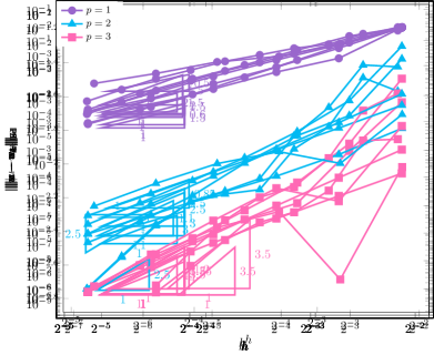
Figure 8.1: Convergence rate plots for the sphere (top) and torus (bottom) test cases with $\epsilon=1$. Both the $L^{2}$ (left) and streamline diffusion (right) error plots show optimal convergence rates.

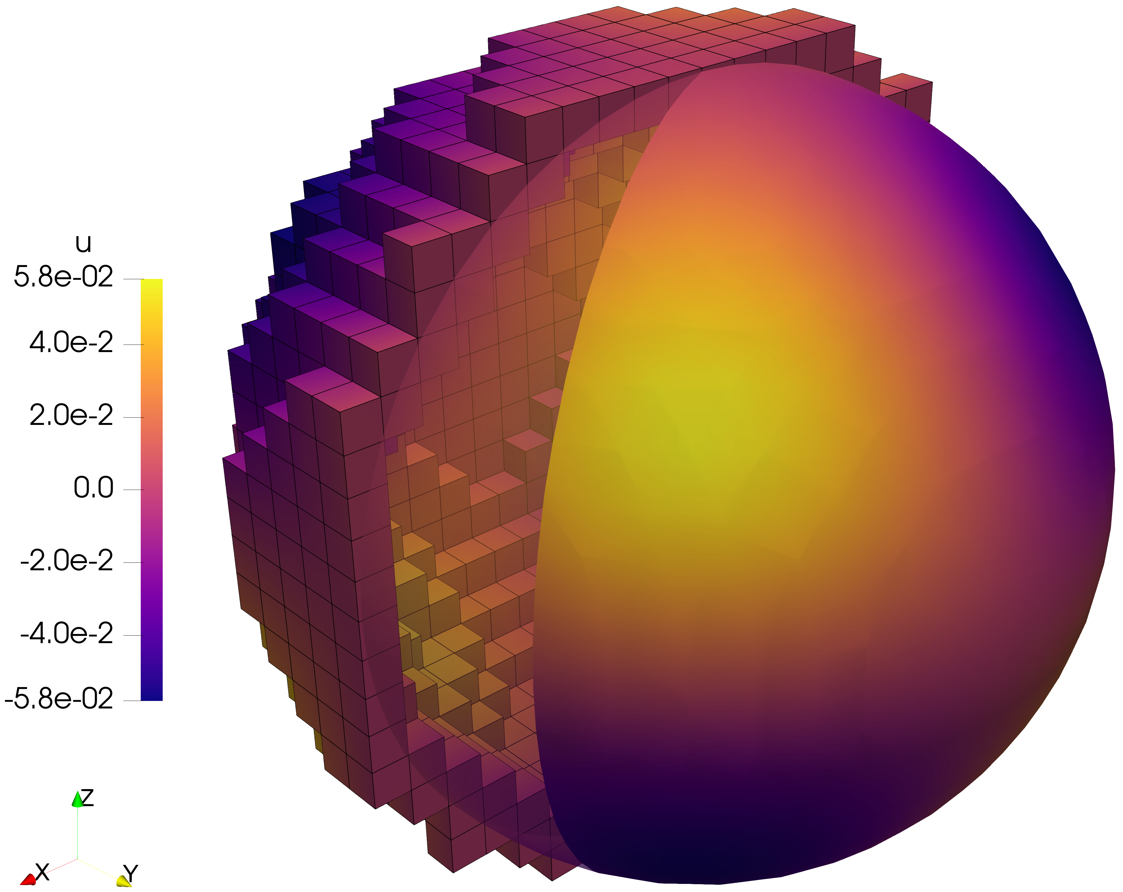
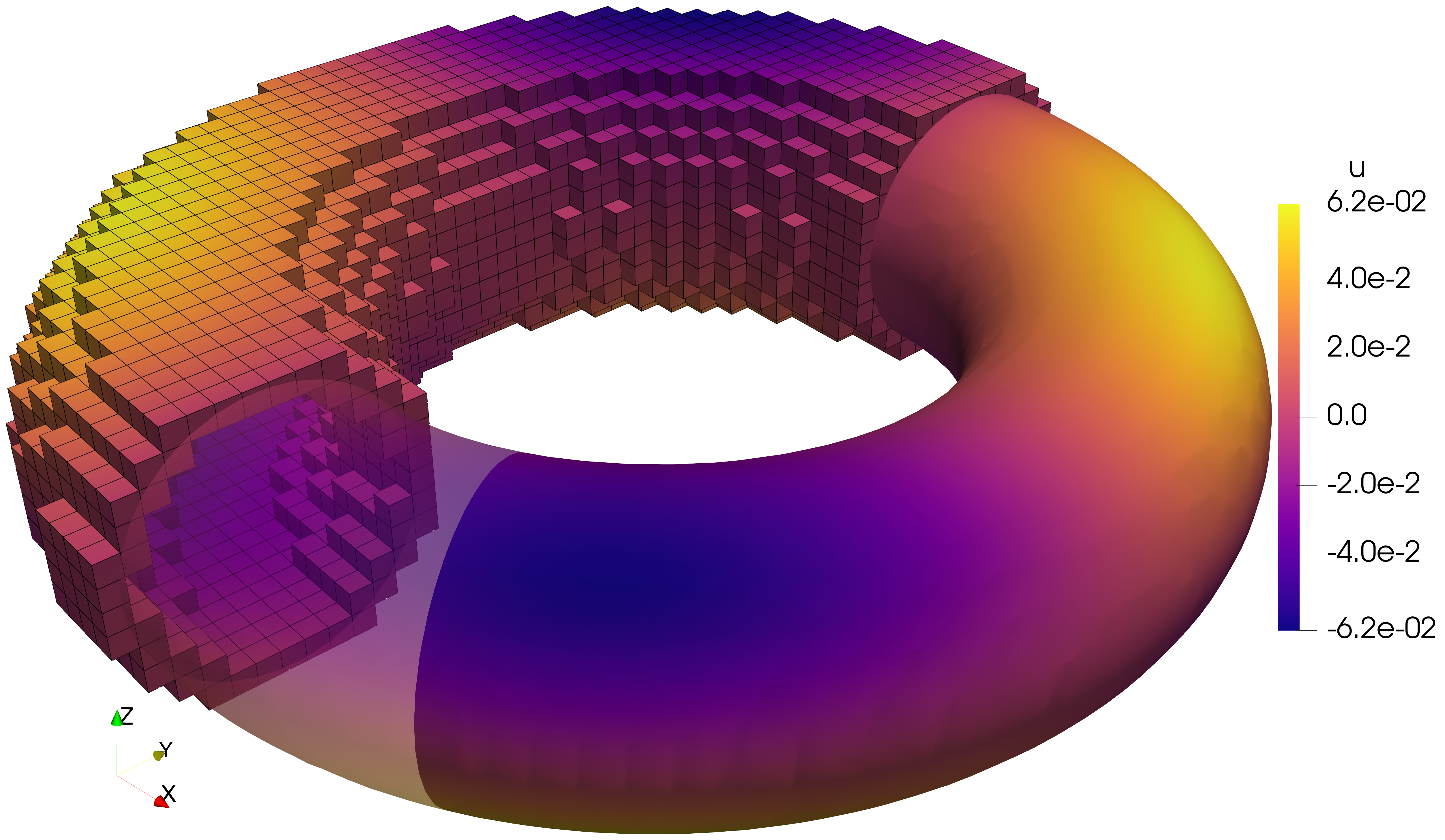
Figure 8.2: Numerical solutions of problem (8.4) with $\epsilon=1$ computed on the unit sphere (left) and torus (right), together with part of the background mesh.

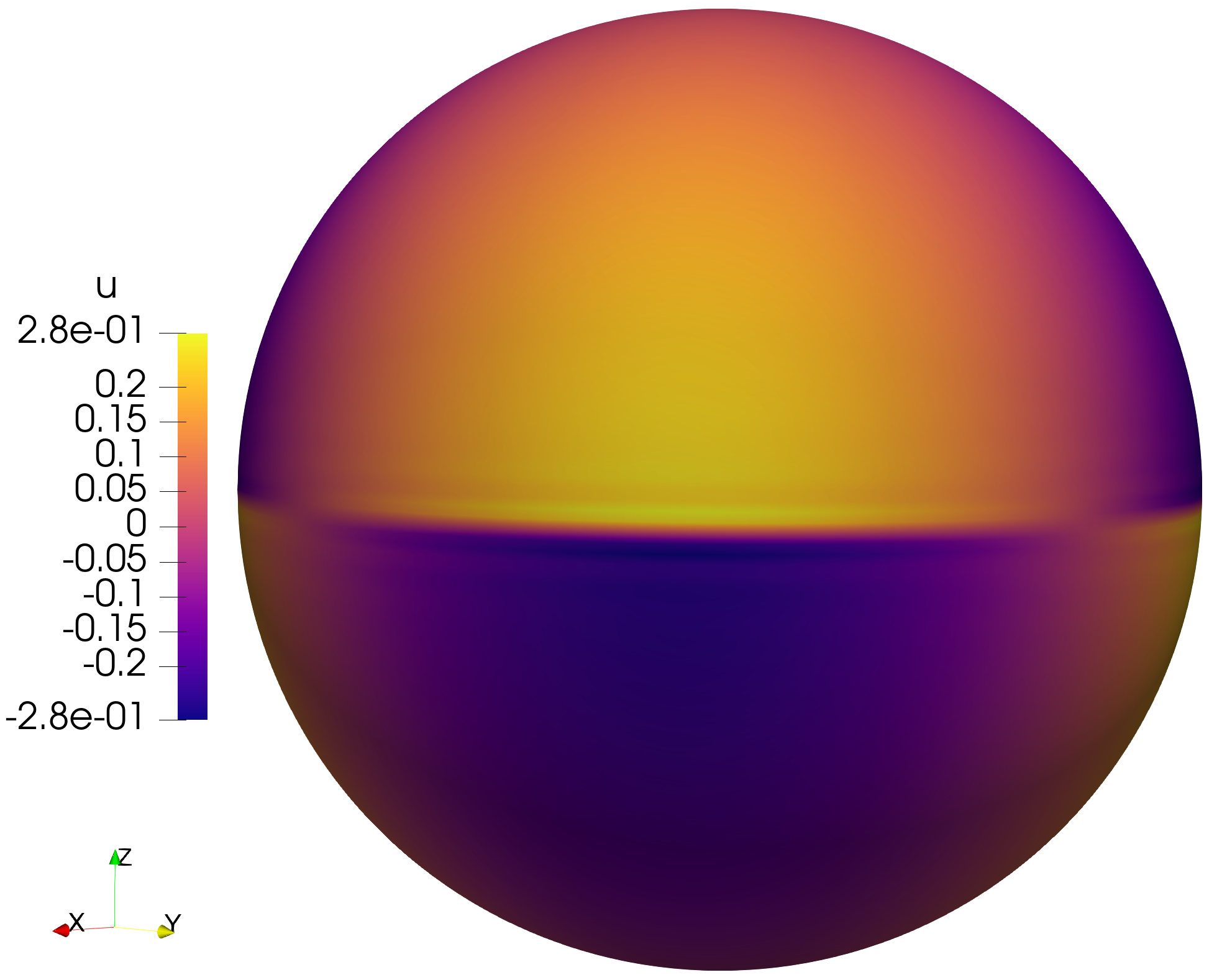
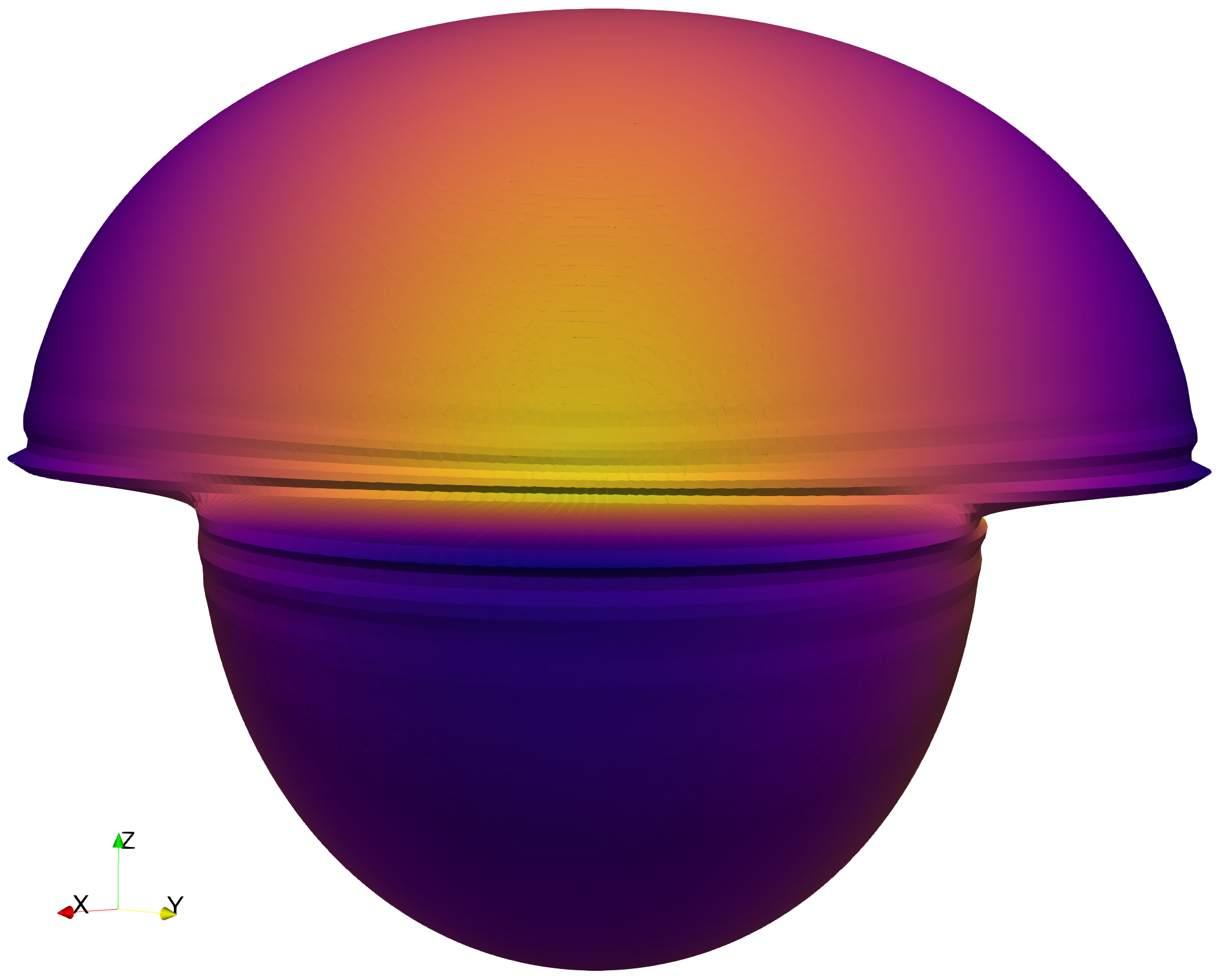
Figure 8.3: Numerical solution of problem (8.4) with $\epsilon=10^{-6}$ computed on the unit sphere (left). Warping the surface $\Gamma$ in the normal direction using the solution $u$ exhibits the strong gradient in the characteristic layer around the equator as well as the localized Gibbs oscillations of the solution (right).

Figure 8.4: Convergence rates in the $L^{2}(\Omega)$ (left) and streamline diffusion (right) norms for the sphere example with $\epsilon=10^{-3}$ (top) and $\epsilon=10^{-6}$ (bottom).

8.2 Condition number

Next, we study the scaling of the condition number $\kappa(\mathcal{A})$ of the system matrix $\mathcal{A}$ with respect to the mesh size $h$ for orders $k\in\{1,2,3\}$. We consider the same experimental setup as for the sphere example. To estimate the condition number for a given mesh $\mathcal{T}_{l}$ and order $k$, we compute numerically the largest and smallest singular value of $\mathcal{A}$ using the SLEPc [82], an open-source library for the solution of large-scale sparse eigenvalue problems which is closely integrated into deal.II. The condition number as a function of mesh size is shown in Figure 8.5, for a few refinements and different orders. Note that since the computation of singular values is computationally heavy and challenging, we were not able to perform equally many condition number calculations for different orders. As expected from Theorem 7.1, we see that the condition number grows proportionally to $h^{-1}$.

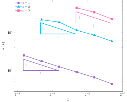
Figure 8.5: Condition number as a function of mesh size, for the test case with $\Gamma$ being a sphere.

8.3 Geometrical robustness

Finally, the last set of numerical experiments is designed to test the geometrical robustness of our proposed CutDG method and to highlight the importance of the ghost penalty.

To test if the method yields robust approximation errors irrespective of the particular cut configuration, we successively compute the numerical solution for the unit sphere test case from the previous section with $\epsilon=1$ while shifting the background mesh by

$$s_{\delta}=\delta\frac{h}{\sqrt{3}}(1,1,1),\quad\delta\in[0,1),$$ (8.6)

Here, $\delta$ is a parameter that quantifies the shift. The problem is solved for $500$ uniformly spaced values of $\delta$ in the interval $[0,1)$ using polynomial order $k=2$. In this interval, the linear system has between $11232$ and $13014$ degrees of freedom. For each sample, we compute both the discretization error measured in the streamline-diffusion norm $|\mspace{-1.0mu}|\mspace{-1.0mu}|\cdot|\mspace{-1.0mu}|\mspace{-1.0mu}|_{\mathrm{sd},h}$ as well as the condition number and plot them against $\delta$, see Figure 8.6. The resulting error sensitivities shown in Figure 8.6 (left) include the results for the “default” parameters (8.1) as well as the results when individual ghost penalty parameters are set to zero. First, we see that when the penalty parameters have the default values from (8.1) the error is independent of $\delta$. When we set $\gamma_{n}=0$, the error fluctuates rapidly and increases by a factor higher than $10^{4}$ at some values of $\delta$. If we instead set $\gamma_{0}=0$, the error is almost the same as for the parameters in (8.1), except for a few spikes, where the error increases significantly. When setting $\gamma_{1}=0$, the error is surprisingly robust and practically constant over $\delta$ but slightly higher than for the parameters in (8.1). It should be noted that, for each $\delta$, the linear system was here solved with an iterative solver (bicgstab). When setting some of the penalty parameters to zero, the linear system might be singular. Thus, what we have presented as the error in Figure 8.6 is the solution from the iterative solver after a maximum of $10^{4}$ iterations, even if the solver did not converge.

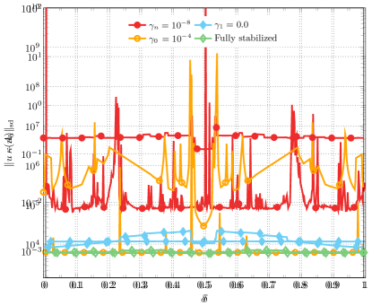
Figure 8.6: Error in $|\mspace{-1.0mu}|\mspace{-1.0mu}|\cdot|\mspace{-1.0mu}|\mspace{-1.0mu}|_{\mathrm{sd}}$-norm (left) and condition number (right) as a function of the mesh perturbation parameter $\delta$ (cf. (8.6)) for different choices of stability parameters.

As expected, the condition number is more mesh-dependent when we significantly decrease the stabilization parameters. When we set $\gamma_{n}=10^{-4}$ the condition number increases by almost 3 orders of magnitude, but is still almost constant. If we instead set $\gamma_{0}=10^{-8}$, we see that the condition number becomes huge and also oscillates rapidly. Here, some values of the condition number are missing. The reason is that the matrix, $\mathcal{A}$, is so ill-conditioned that the used singular value solver did not converge when solving for the smallest singular value. Of the various penalty parameters, $\gamma_{1}$ appears to be the one that has the smallest effect. When we set $\gamma_{1}=0$ we see that the condition number becomes slightly more mesh-dependent compared to the parameters in (8.1), but the variation is very slight.

9 Conclusion and outlook

In this paper, we proposed a novel cut discontinuous Galerkin method for stationary advection-reaction problems on surfaces. Our main goal was to generalize the classical upwind-flux DG formulation to the setting of embedded surfaces by extending ideas from the stabilized, continuous Galerkin-based CutFEM framework [20, 21] for surface PDEs. We carefully designed suitable stabilization forms for higher-order DG methods which allowed us to establish geometrically robust stability, a priori error, and condition number estimates by using enhanced $L^{2}$ and streamline-diffusion type norms. Moreover, the presented stabilization approach allows for a relatively easy extension of existing fitted discontinuous Galerkin software to handle unfitted geometries. Implementation of the stabilization operator (5.30) should be straight-forward in most DG software frameworks, and thus only additional quadrature routines such as [83, 84, 85, 86, 87] are needed to handle the numerical integration on cut geometries.

In this work, we focused on the prototype problems (2.8) to lay out the main ideas in the simplest possible setting, but our method can be readily employed in more complex simulation scenarios, including advection-dominated advection-diffusion-reaction problems on surfaces when combined with [58], or for corresponding mixed-dimensional problems in combination with  [59, 71, 72]. In [72] we already outlined relevant extensions and research directions for the proposed stabilized CutDG formulation for advection-dominated bulk problems. In particular, we demonstrated how the stabilization approach can be combined with explicit Runge–Kutta methods to solve the time-dependent advection-reaction problem under a standard hyperbolic CFL condition. The research directions and method extensions from [72] are equally applicable to CutDG formulation in this work. It is part of our ongoing research to combine the presented stabilized CutDG framework with the general symmetric stabilization approach proposed in [88] to devise an explicit Runge–Kutta method for first-order Friedrichs-type operators covering advection-reaction problems as well as linear wave propagation phenomena.

Moreover, for the numerical discretization of nonlinear scalar hyperbolic conservation laws on surfaces, a major research question is to understand how our proposed CutDG stabilization can be combined with the discontinuous Galerkin Runge–Kutta methods originally developed in [89, 90, 91, 92]. To maintain properties such as local conservation, monotonicity, total variation diminishing (TVD) stability often required from numerical methods for hyperbolic conservation laws, modifications of the proposed stabilizations need to be developed. Here, it would be interesting to investigate whether and how the approaches developed in [93, 94] can be carried over to the setting of embedded surfaces.

Appendix A Proofs of some geometric estimates

Proof 14 (Lemma 4.3)

To establish (4.38), we simply combine estimates (4.27), (4.28), and 4.32 to obtain

$$\||B|B^{-1}b^{e}-b_{h}\|_{L^{\infty}(\mathcal{K}_{h})} \lesssim\||B|B^{-1}b^{e}-B^{-1}b^{e}\|_{L^{\infty}(\mathcal{K}_{h})}+\|B^{-1}b^{e}-b_{h}\|_{L^{\infty}(\mathcal{K}_{h})}$$ (A.1)

$$\lesssim\||B|-1\|_{L^{\infty}(\mathcal{K}_{h})}\|B^{-1}b^{e}\|_{L^{\infty}(\mathcal{K}_{h})}+\|B^{-1}b^{e}-b_{h}\|_{L^{\infty}(\mathcal{K}_{h})}$$ (A.2)

$$\lesssim h^{k_{g}+1}+\|B^{-1}b^{e}-b_{h}\|_{L^{\infty}(\mathcal{K}_{h})}$$ (A.3)

$$\lesssim h^{k_{g}+1}+\|(B^{-1}-{P}_{\Gamma_{h}}{P}_{\Gamma})b^{e}\|_{L^{\infty}(\mathcal{K}_{h})}+\|{P}_{\Gamma_{h}}{P}_{\Gamma}b^{e}-b_{h}\|_{L^{\infty}(\mathcal{K}_{h})}$$ (A.4)

$$\lesssim h^{k_{g}+1}+\|{P}_{\Gamma_{h}}b^{e}-b_{h}\|_{L^{\infty}(\mathcal{K}_{h})}.$$ (A.5)

Inequalities (4.39) and (4.40) can be proved similarly.

Proof 15 (Lemma 4.4)

We start the proof by noting that in contrast to their discrete counterparts $n_{E}^{\pm}$, the two co-normal fields $n_{E^{l}}^{\pm}(x)\in T_{x}\Gamma$ associated with the lifted edge $E^{l}$ are in fact co-planar and satisfy $n_{E^{l}}^{+}=-n_{E^{l}}^{-}$ and hence $[b^{e};n_{E^{l}}^{e}]=0$. Thus

$$\|[b_{h};n_{E}]\|_{L^{\infty}(\mathcal{E}_{h})}\leqslant\|[b_{h}-b^{e};n_{E}]\|_{L^{\infty}(\mathcal{E}_{h})}+\|[b^{e};n_{E}-n_{E_{l}}^{e}]\|_{L^{\infty}(\mathcal{E}_{h})}=I+II.$$ (A.6)

To estimate $I$, simply observe that $b^{e,\pm}\cdot n_{E}^{\pm}=({P}_{\Gamma_{h}}b^{e})^{\pm}\cdot n_{E}^{\pm}$, which thanks to assumption (4.32) implies that

$$I \lesssim\|(b_{h}-{P}_{\Gamma_{h}}b^{e})^{+}\cdot n_{E}^{+}]\|_{L^{\infty}(\mathcal{E}_{h})}+\|(b_{h}-{P}_{\Gamma_{h}}b^{e})^{-}\cdot n_{E}^{-}]\|_{L^{\infty}(\mathcal{E}_{h})}\lesssim C_{b}h^{k_{g}+1}.$$ (A.7)

Next, using the fact that $b^{e}\cdot n_{E}^{\pm}={P}_{\Gamma}^{e}b^{e}\cdot n_{E}^{\pm}=b^{e}\cdot{P}_{\Gamma}^{e}n_{E}^{\pm}$ thanks to the self-adjointness of ${P}_{\Gamma}$, the remaining term $II$ can be bound by

$$II \leqslant\|b^{e}\cdot({P}_{\Gamma}^{e}n_{E}^{+}-n_{E^{l}}^{+,e})\|_{L^{\infty}(\Gamma_{h})}+\|b^{e}\cdot({P}_{\Gamma}^{e}n_{E}^{-}-n_{E^{l}}^{-,e})\|_{L^{\infty}(\Gamma_{h})}=II_{a}+II_{b}.$$ (A.8)

Clearly, it is sufficient to provide an estimate for $II_{a}\leqslant b_{c}\|{P}_{\Gamma}^{e}n_{E}^{+}-n_{E^{l}}^{+,e}\|_{L^{\infty}(\Gamma_{h})}$ since $II_{b}$ can be handled in the exact same manner. We introduce a moving orthonormal basis $t_{1}(x),\ldots,t_{d-1}(x)\in T_{x}E$ such that $\{t_{1},\ldots,t_{d-1},n_{E},n_{\Gamma_{h}}\}$ is a positively oriented orthonormal basis of $\mathbb{R}^{d+1}$. Then $-n_{E}=t_{1}\wedge t_{2}\wedge\ldots\wedge t_{d-1}\wedge n_{\Gamma_{h}}$. Here and in the following, we omit the superscripts ^± and ^e to ease the notation. After a rigid motion, we can safely assume that $\{t_{1},\ldots,t_{d-1},n_{E},n_{\Gamma_{h}}\}=\{e_{1},\ldots,e_{d-1},e_{d},e_{d+1}\}$. Note that in this orthonormal basis, we have that $n_{\Gamma}^{i}=n_{\Gamma}\cdot e_{i}=(n_{\Gamma}-n_{\Gamma_{h}})\cdot e_{i}=\mathcal{O}(h^{k_{g}})$ for $i=1,\ldots,d$ and hence $n_{\Gamma}^{d+1}=\sqrt{1+\mathcal{O}(h^{2k_{g}})}=1+\mathcal{O}(h^{2k_{g}})$. Now we expand ${P}_{\Gamma}n_{E}={P}_{\Gamma}e_{d}$ in the chosen orthonormal basis leading to

$${P}_{\Gamma}e_{d}\cdot e_{i}=\delta_{d,i}-n_{\Gamma}^{d}n_{\Gamma}^{i}=\begin{cases}\mathcal{O}(h^{2k_{g}}),&i=1,\ldots,d-1\\ 1+\mathcal{O}(h^{2k_{g}}),&i=d\\ -n_{\Gamma}^{d}n_{\Gamma}^{d+1},&i=d+1.\end{cases}$$ (A.9)

Next, using the differential $Dp={P}_{\Gamma}(\operatorname{Id}-\rho\mathcal{H}){P}_{\Gamma_{h}}$ of the closest point projection $p$, we define

$$-\widetilde{n}_{E^{l}}=Dpe_{1}\wedge Dpe_{2}\wedge Dpe_{d-1}\wedge n_{\Gamma},$$ (A.10)

which is a non-normalized, outward pointing co-normal field on the lifted edge $E^{l}$; that is, $n_{E^{l}}=\lambda\widetilde{n}_{E^{l}}$ for some $\lambda>0$. Recalling the general definition of the outer product, we see that

$$-\widetilde{n}_{E^{l}}\cdot e_{i} =\det(Dpe_{1},Dpe_{2},Dpe_{d-1},n_{\Gamma},e_{i})$$ (A.11)

$$=\det({P}_{\Gamma}e_{1},{P}_{\Gamma}e_{2},{P}_{\Gamma}e_{d-1},n_{\Gamma},e_{i})+\mathcal{O}(h^{k_{g}+1})$$ (A.12)

$$=\det(e_{1},e_{2},e_{d-1},n_{\Gamma},e_{i})+\mathcal{O}(h^{k_{g}+1})$$ (A.13)

$$=\begin{cases}0+\mathcal{O}(h^{k_{g}+1})&i=1,\ldots,d-1\\ -n_{\Gamma}^{d+1}+\mathcal{O}(h^{k_{g}+1})=-1+\mathcal{O}(h^{k_{g}+1})&i=d\\ n_{\Gamma}^{d}+\mathcal{O}(h^{k_{g}+1})&i=d+1.\end{cases}$$ (A.14)

As all coefficients scale like at least $\mathcal{O}(h^{k_{g}})$ except for $i=d$, we see that $\|\widetilde{n}_{E^{l}}\|_{\mathbb{R}^{d+1}}=1+\mathcal{O}(h^{2k_{g}})$, hence $\lambda=\|\widetilde{n}_{E^{l}}\|_{\mathbb{R}^{d+1}}^{-1}=1+\mathcal{O}(h^{2k_{g}})$ and consequently we obtain the following estimates for the coefficients of $n_{E^{l}}$ with respect to the orthonormal base $\{e_{1}\ldots,e_{d+1}\}$,

$$-n_{E^{l}}=-\lambda\widetilde{n}_{E^{l}}=-(1+\mathcal{O}(h^{2k_{g}}))\widetilde{n}_{E^{l}} =\begin{cases}0+\mathcal{O}(h^{k_{g}+1})&i=1,\ldots,d-1\\ -1+\mathcal{O}(h^{k_{g}+1})&i=d,\\ n_{\Gamma}^{d}+\mathcal{O}(h^{k_{g}+1})&i=d+1.\end{cases}$$ (A.15)

As a result, comparing (A.9) and (A.15) yields

$$({P}_{\Gamma}e_{d}-n_{E^{l}}^{e})\cdot e_{i}=\begin{cases}\mathcal{O}(h^{k_{g}+1})&i=1,\ldots,d\\ n_{\Gamma}^{d}(1-n_{\Gamma}^{d+1})+\mathcal{O}(h^{k_{g}+1})=\mathcal{O}(h^{k_{g}+1}),&i=d+1,\end{cases}$$ (A.16)

which immediately implies that $II_{a}\leqslant b_{c}h^{k_{g}+1}$. This concludes the proof.

References

- Alboin et al. [2002] C. Alboin, J. Jaffré, J. E. Roberts, C. Serres, Modeling fractures as interfaces for flow and transport, Fluid Flow and Transport in Porous Media, Mathematical and Numerical Treatment 295 (2002) 13. doi:10/fzhstf.
- Adler et al. [2012] P. M. Adler, J.-F. Thovert, V. V. Mourzenko, Fractured Porous Media, Oxford University Press, 2012. doi:10.1093/acprof:oso/9780199666515.001.0001.
- Fumagalli [2012] A. Fumagalli, Numerical Modelling of Flows in Fractured Porous Media by the XFEM Method, Ph.D. thesis, Italy, 2012.
- Burman et al. [2019] E. Burman, P. Hansbo, M. G. Larson, K. Larsson, Cut finite elements for convection in fractured domains, Comput. Fluids 179 (2019) 726–734. doi:10/gd8mhw.
- Ganesan and Tobiska [2009] S. Ganesan, L. Tobiska, A coupled arbitrary Lagrangian–Eulerian and Lagrangian method for computation of free surface flows with insoluble surfactants, J. Comput. Phys. 228 (2009) 2859–2873. doi:10/cjpt48.
- Gross and Reusken [2011] S. Gross, A. Reusken, Numerical Methods for Two-phase Incompressible Flows, volume 40 of Springer Series in Computational Mathematics, Springer, Berlin, Heidelberg, 2011. doi:10.1007/978-3-642-19686-7.
- Muradoglu and Tryggvason [2008] M. Muradoglu, G. Tryggvason, A front-tracking method for computation of interfacial flows with soluble surfactants, J. Comput. Phys. 227 (2008) 2238–2262. doi:10/fdrg2m.
- Groß and Reusken [2013] S. Groß, A. Reusken, Numerical simulation of continuum models for fluid-fluid interface dynamics, Eur. Phys. J. Special Topics 222 (2013) 211–239. doi:10/f43kkj.
- Agrawal and Neuman [1988] M. Agrawal, R. D. Neuman, Surface diffusion in monomolecular films: II. Experiment and theory, J. Colloid Interface Sci. 121 (1988) 366–380. doi:10/bjz5sx.
- Burman et al. [2015] E. Burman, S. Claus, P. Hansbo, M. G. Larson, A. Massing, CutFEM: Discretizing geometry and partial differential equations, Int. J. Numer. Meth. Engng. 104 (2015) 472–501. doi:10.1002/nme.4823.
- Bordas et al. [2018] S. Bordas, E. Burman, M. Larson, M. Olshanskii (Eds.), Geometrically Unfitted Finite Element Methods and Applications, Springer, 2018.
- Olshanskii et al. [2009] M. A. Olshanskii, A. Reusken, J. Grande, A finite element method for elliptic equations on surfaces, SIAM J. Numer. Anal. 47 (2009) 3339–3358. doi:10/bh2h32.
- Dziuk [1988] G. Dziuk, Finite elements for the Beltrami operator on arbitrary surfaces, in: Partial Differential Equations and Calculus of Variations, volume 1357 of Lecture Notes in Math., Springer, Berlin, 1988, pp. 142–155.
- Dziuk and Elliott [2013] G. Dziuk, C. M. Elliott, Finite element methods for surface PDEs, Acta Numer. 22 (2013) 289–396. doi:10/ggzzsq.
- Bonito and Nochetto [2020] A. Bonito, R. H. Nochetto (Eds.), Geometric Partial Differential Equations - Part I, volume 21 of Handbook of Numerical Analysis, 2020.
- Grande and Reusken [2016] J. Grande, A. Reusken, A higher order finite element method for partial differential equations on surfaces, SIAM J. Numer. Anal. 54 (2016) 388–414. doi:10/f8cp8n.
- Reusken [2014] A. Reusken, Analysis of trace finite element methods for surface partial differential equations, IMA J. Numer. Anal. 35 (2014) 1568–1590. doi:10.1093/imanum/dru047.
- Burman et al. [2015] E. Burman, P. Hansbo, M. G. Larson, A stabilized cut finite element method for partial differential equations on surfaces: The Laplace–Beltrami operator, Comput. Methods Appl. Mech. Engrg. 285 (2015) 188–207. doi:10/f24rp2.
- Burman et al. [2016] E. Burman, P. Hansbo, M. G. Larson, A. Massing, S. Zahedi, Full gradient stabilized cut finite element methods for surface partial differential equations, Comput. Methods Appl. Mech. Engrg. 310 (2016) 278–296. doi:10/f3rzs9.
- Grande et al. [2018] J. Grande, C. Lehrenfeld, A. Reusken, Analysis of a high-order trace finite element method for PDEs on level set surfaces, SIAM J. Numer. Anal. 56 (2018) 228–255. doi:10/gdb8m4.
- Burman et al. [2018] E. Burman, P. Hansbo, M. G. Larson, A. Massing, Cut finite element methods for partial differential equations on embedded manifolds of arbitrary codimensions, ESAIM: Math. Model. Numer. Anal. 52 (2018) 2247–2282. doi:10/gh8jr6.
- Hansbo et al. [2017] P. Hansbo, M. G. Larson, A. Massing, A stabilized cut finite element method for the Darcy problem on surfaces, Comput. Methods Appl. Math. 326 (2017) 298–318. doi:10/gbvxj7.
- Olshanskii et al. [2018] M. A. Olshanskii, A. Quaini, A. Reusken, V. Yushutin, A finite element method for the surface Stokes problem, SIAM J. Sci. Comput. 40 (2018) A2492–A2518. doi:10/grm2jb.
- Olshanskii et al. [2021] M. A. Olshanskii, A. Reusken, A. Zhiliakov, Inf-sup stability of the trace P2-P1 Taylor-Hood elements for surface PDEs, Math. Comput. 90 (2021) 1527–1555. doi:10/grm2gq.
- Dziuk and Elliott [2007] G. Dziuk, C. M. Elliott, Finite elements on evolving surfaces, IMA J. Numer. Anal. 27 (2007) 262–292. doi:10/c4x9hd.
- Elliott et al. [2010] C. M. Elliott, B. Stinner, V. Styles, R. Welford, Numerical computation of advection and diffusion on evolving diffuse interfaces, IMA J. Numer. Anal. 31 (2010) 786–812. doi:10/fvwjsz.
- Olshanskii and Reusken [2014] M. A. Olshanskii, A. Reusken, Error analysis of a space-time finite element method for solving PDEs on evolving surfaces, SIAM J. Numer. Anal. 52 (2014) 2092–2120. doi:10/f6gc3m.
- Olshanskii et al. [2014] M. A. Olshanskii, A. Reusken, X. Xu, An Eulerian space-time finite element method for diffusion problems on evolving surfaces, SIAM J. Numer. Anal. 52 (2014) 1354–1377. doi:10/f585nm.
- Lehrenfeld et al. [2018] C. Lehrenfeld, M. A. Olshanskii, X. Xu, A stabilized trace finite element method for partial differential equations on evolving surfaces, SIAM J. Numer. Anal. 56 (2018) 1643–1672. doi:10/grm2gs.
- Zahedi [2017] S. Zahedi, A space-time cut finite element method with quadrature in time, in: S. P. A. Bordas, E. Burman, M. G. Larson, M. A. Olshanskii (Eds.), Geometrically Unfitted Finite Element Methods and Applications, Springer International Publishing, Cham, 2017, pp. 281–306.
- Kovács [2017] B. Kovács, High-order evolving surface finite element method for parabolic problems on evolving surfaces, IMA J. Numer. Anal. (2017) drx013. doi:10/grm2g2.
- Roos et al. [2008] H.-G. Roos, M. Stynes, L. Tobiska, Robust Numerical Methods for Singularly Perturbed Differential Equations: Convection-Diffusion-Reaction and Flow Problems, volume 24, Springer Science & Business Media, 2008.
- Ern and Guermond [2021] A. Ern, J.-L. Guermond, Finite Elements III: First-order and Time-Dependent PDEs, volume 74 of Texts in Applied Mathematics, Springer Nature, 2021.
- Olshanskii et al. [2014] M. A. Olshanskii, A. Reusken, X. Xu, A stabilized finite element method for advection–diffusion equations on surfaces, IMA J. Numer. Anal. 34 (2014) 732–758. doi:10/f5zf9x.
- Hansbo et al. [2015] P. Hansbo, M. G. Larson, S. Zahedi, Characteristic cut finite element methods for convection–diffusion problems on time dependent surfaces, Comput. Methods Appl. Mech. Engrg. 293 (2015) 431–461. doi:10/f3pbxn.
- Burman et al. [2019] E. Burman, P. Hansbo, M. G. Larson, S. Zahedi, Stabilized CutFEM for the convection problem on surfaces, Numer. Math. 141 (2019).
- Burman et al. [2020] E. Burman, P. Hansbo, M. G. Larson, A. Massing, S. Zahedi, A stabilized cut streamline diffusion finite element method for convection–diffusion problems on surfaces, Comput. Methods Appl. Mech. Engrg. 358 (2020) 112645. doi:10/gf8vwp.
- Chernyshenko and Olshanskii [2015] A. Y. Chernyshenko, M. A. Olshanskii, An adaptive octree finite element method for PDEs posed on surfaces, Comput. Methods Appl. Mech. Engrg. 291 (2015) 146–172.
- Simon [2017] K. Simon, Higher Order Stabilized Surface Finite Element Methods for Diffusion-Convection-Reaction Equations on Surfaces with and without Boundary, Ph.D. thesis, 2017.
- Simon and Tobiska [2019] K. Simon, L. Tobiska, Local projection stabilization for convection–diffusion–reaction equations on surfaces, Comput. Methods Appl. Mech. Engrg. 344 (2019) 34–53. doi:10/grm2gx.
- Bachini et al. [2021] E. Bachini, M. W. Farthing, M. Putti, Intrinsic finite element method for advection-diffusion-reaction equations on surfaces, J. Comput. Phys. 424 (2021) 109827. doi:10/grm2gr.
- Zhao et al. [2020] S. Zhao, X. Xiao, J. Zhao, X. Feng, A Petrov-Galerkin finite element method for simulating chemotaxis models on stationary surfaces, Comput. Math. Appl. 79 (2020) 3189–3205. doi:10/grm2gk.
- Reed and Hill [1973] W. Reed, T. Hill, Triangular mesh methods for the neutron transport equation, Technical Report LA-UR-73-479, Los Alamos Scientific Laboratory, Los Alamos, NM (1973).
- Lesaint and Raviart [1974] P. Lesaint, P. Raviart, On a finite element method for solving the neutron transport equation. In: Mathematical aspects of finite elements in partial differential equations (proc. Sympos., math. Res.Center, univ. Wisconsin, madison, wis., 1974), Academic Press, New York 33 (1974) 89–123.
- Johnson et al. [1984] C. Johnson, U. Nävert, J. Pitkäranta, Finite element methods for linear hyperbolic problems, Comput. Methods Appl. Mech. Engrg. 45 (1984) 285–312.
- Brezzi et al. [2004] F. Brezzi, L. D. Marini, E. Süli, Discontinuous Galerkin methods for first-order hyperbolic problems, Math. Models Methods Appl. Sci. 14 (2004) 1893–1903. doi:10/ddbp5h.
- Cockburn [1999] B. Cockburn, Discontinuous Galerkin methods for convection-dominated problems, High Order Methods for Computational Physics, Lect. Notes Comput. Sci. Eng. 9 (1999) 69–224.
- Houston et al. [2002] P. Houston, C. Schwab, E. Süli, Discontinuous hp-finite element methods for advection-diffusion-reaction problems, SIAM J. Numer. Anal. 39 (2002) 2133–2163. doi:10/d9h397.
- Zarin and Roos [2005] H. Zarin, H.-G. Roos, Interior penalty discontinuous approximations of convection–diffusion problems with parabolic layers, Numer. Math. 100 (2005) 735–759. doi:10/fdrvfc.
- Arnold et al. [2002] D. Arnold, F. Brezzi, B. Cockburn, L. Marini, Unified analysis of discontinuous Galerkin methods for elliptic problems, SIAM J. Numer. Anal. 39 (2002) 1749–1779. doi:10/cdb548.
- Arnold et al. [2000] D. N. Arnold, F. Brezzi, B. Cockburn, L. Marini, Discontinuous Galerkin approximations for elliptic problems, Numer. Methods Partial Differential Equations 16 (2000) 365–378. doi:10/fwvfmc.
- Di Pietro and Ern [2012] D. A. Di Pietro, A. Ern, Mathematical Aspects of Discontinuous Galerkin Methods, volume 69, Springer, 2012.
- Hesthaven and Warburton [2007] J. S. Hesthaven, T. Warburton, Nodal Discontinuous Galerkin Methods: Algorithms, Analysis, and Applications, Springer Science & Business Media, 2007.
- Dedner and Madhavan [2015] A. Dedner, P. Madhavan, Discontinuous Galerkin methods for hyperbolic and advection-dominated problems on surfaces, ArXiv e-prints (2015). doi:10/grm2g4.
- Dedner et al. [2013] A. Dedner, P. Madhavan, B. Stinner, Analysis of the discontinuous Galerkin method for elliptic problems on surfaces, IMA J. Numer. Anal. 33 (2013) 952–973.
- Antonietti et al. [2015] P. F. Antonietti, A. Dedner, P. Madhavan, S. Stangalino, B. Stinner, M. Verani, High order discontinuous galerkin methods for elliptic problems on surfaces, SIAM J. Numer. Anal. 53 (2015) 1145–1171. doi:10/f694jc.
- Cockburn and Demlow [2016] B. Cockburn, A. Demlow, Hybridizable discontinuous Galerkin and mixed finite element methods for elliptic problems on surfaces, Math. Comp. (2016). doi:10/grm2gw.
- Burman et al. [2016] E. Burman, P. Hansbo, M. G. Larson, A. Massing, A cut discontinuous Galerkin method for the Laplace–Beltrami operator, IMA J. Numer. Anal. 37 (2016) 138–169. doi:10/f3t2wk.
- Massing [2017] A. Massing, A cut discontinuous Galerkin method for coupled bulk-surface problems, in: Geometrically Unfitted Finite Element Methods and Applications, Lecture Notes in Computational Science and Engineering, Springer, 2017, pp. 259–279.
- Larson and Zahedi [2021] M. G. Larson, S. Zahedi, Conservative Discontinuous Cut Finite Element Methods, Technical Report, arXiv, 2021. doi:10.48550/ARXIV.2105.02202.
- Bastian and Engwer [2009] P. Bastian, C. Engwer, An unfitted finite element method using discontinuous Galerkin, Internat. J. Numer. Meth. Engrg 79 (2009) 1557–1576. doi:10.1002/nme.2631.
- Bastian et al. [2011] P. Bastian, C. Engwer, J. Fahlke, O. Ippisch, An Unfitted Discontinuous Galerkin method for pore-scale simulations of solute transport, Math. Comput. Simul 81 (2011) 2051–2061. doi:10/ffx48t.
- Sollie et al. [2011] W. E. H. Sollie, O. Bokhove, J. J. W. van der Vegt, Space–time discontinuous Galerkin finite element method for two-fluid flows, J. Comput. Phys. 230 (2011) 789–817. doi:10/dv427m.
- Heimann et al. [2013] F. Heimann, C. Engwer, O. Ippisch, P. Bastian, An unfitted interior penalty discontinuous Galerkin method for incompressible Navier–Stokes two–phase flow, Internat. J. Numer. Methods Fluids 71 (2013) 269–293. doi:10/f4kcxw.
- Saye [2017a] R. Saye, Implicit mesh discontinuous Galerkin methods and interfacial gauge methods for high-order accurate interface dynamics, with applications to surface tension dynamics, rigid body fluid-structure interaction, and free surface flow: Part I, J. Comput. Phys. 344 (2017a) 647–682. doi:10.1016/j.jcp.2017.04.076.
- Saye [2017b] R. Saye, Implicit mesh discontinuous Galerkin methods and interfacial gauge methods for high-order accurate interface dynamics, with applications to surface tension dynamics, rigid body fluid-structure interaction, and free surface flow: Part II, J. Comput. Phys. 344 (2017b) 683–723. doi:10.1016/j.jcp.2017.05.003.
- Müller et al. [2016] B. Müller, S. Krämer-Eis, F. Kummer, M. Oberlack, A high-order Discontinuous Galerkin method for compressible flows with immersed boundaries, Int. J. Numer. Methods Eng. 110 (2016) 3–30. doi:10/f9zvph.
- Krause and Kummer [2017] D. Krause, F. Kummer, An incompressible immersed boundary solver for moving body flows using a cut cell discontinuous Galerkin method, Comput. Fluids 153 (2017) 118–129. doi:10/gbj9f5.
- Massjung [2012] R. Massjung, An unfitted discontinuous Galerkin method applied to elliptic interface problems, SIAM J. Numer. Anal. 50 (2012) 3134–3162. doi:10/grm2gv.
- Johansson and Larson [2013] A. Johansson, M. Larson, A high order discontinuous Galerkin Nitsche method for elliptic problems with fictitious boundary, Numer. Math. 123 (2013) 607–628. doi:10/f22sp5.
- Gürkan and Massing [2019] C. Gürkan, A. Massing, A stabilized cut discontinuous Galerkin framework for elliptic boundary value and interface problems, Comput. Methods Appl. Mech. Engrg. 348 (2019) 466–499. doi:10/gfv5sj.
- Gürkan et al. [2020] C. Gürkan, S. Sticko, A. Massing, Stabilized cut discontinuous galerkin methods for advection-reaction problems, SIAM J. Sci. Comput. 42 (2020) A2620–A2654. doi:10/gjd6vv.
- Hansbo et al. [2003] A. Hansbo, P. Hansbo, M. G. Larson, A finite element method on composite grids based on Nitsche’s method, ESAIM: Math. Model. Numer. Anal. 37 (2003) 495–514. doi:10/bgbqb9.
- Evans and Gariepy [2015] L. C. Evans, R. F. Gariepy, Measure Theory and Fine Properties of Functions, Revised Edition, 2015.
- Burman and Ern [2007] E. Burman, A. Ern, Continuous interior penalty hp-finite element methods for advection and advection-diffusion equations, Math. Comp. 76 (2007) 1119–1140. doi:10/cng2z2.
- Larson and Zahedi [2019] M. G. Larson, S. Zahedi, Stabilization of high order cut finite element methods on surfaces, IMA J. Numer. Anal. 40 (2019) 1702–1745. doi:10/gh99kb.
- Ern and Guermond [2006] A. Ern, J.-L. Guermond, Evaluation of the condition number in linear systems arising in finite element approximations, ESAIM: Math. Model. Numer. Anal. 40 (2006) 29–48. doi:10/fxbx9k.
- Arndt et al. [2022] D. Arndt, W. B. M. Feder, M. Fehling, R. Gassmöller, T. Heister, L. Heltai, M. Kronbichler, M. Maier, P. Munch, J.-P. Pelteret, S. Sticko, B. Turcksin, D. Wells, The deal.II library, version 9.4, J. Numer. Math. (2022). doi:10/gqnpqq.
- Peterson [1991] T. E. Peterson, A note on the convergence of the discontinuous Galerkin method for a scalar hyperbolic equation, SIAM J. Numer. Anal. 28 (1991) 133–140. doi:10/fb4mvb.
- Shu [2009] C.-W. Shu, High order weighted essentially nonoscillatory schemes for convection dominated problems, SIAM Rev. 51 (2009) 82–126. doi:10/dsdhjg.
- Shu [2016] C.-W. Shu, High order WENO and DG methods for time-dependent convection-dominated PDEs: A brief survey of several recent developments, J. Comput. Phys. 316 (2016) 598–613. doi:10/ggrbcg.
- Hernandez et al. [2005] V. Hernandez, J. E. Roman, V. Vidal, SLEPc: A scalable and flexible toolkit for the solution of eigenvalue problems, ACM Trans. Math. Software 31 (2005) 351–362. doi:10/fmqhxx.
- Müller et al. [2013] B. Müller, F. Kummer, M. Oberlack, Highly accurate surface and volume integration on implicit domains by means of moment-fitting, Internat. J. Numer. Meth. Engrg 6 (2013) 10–16. doi:10.1002/nme.4569.
- Saye [2015] R. I. Saye, High-order quadrature methods for implicitly defined surfaces and volumes in hyperrectangles, SIAM J. Sci. Comput. 37 (2015) A993–A1019. doi:10/f7bzzt.
- Lehrenfeld [2016] C. Lehrenfeld, High order unfitted finite element methods on level set domains using isoparametric mappings, Comput. Methods Appl. Mech. Engrg. 300 (2016) 716–733. doi:10/f78gs3.
- Fries and Omerović [2016] T.-P. Fries, S. Omerović, Higher-order accurate integration of implicit geometries, Int. J. Numer. Methods Eng. 106 (2016) 323–371. doi:10/f8gzjs.
- Fries et al. [2017] TP. Fries, S. Omerović, D. Schöllhammer, J. Steidl, Higher-order meshing of implicit geometries—Part I: Integration and interpolation in cut elements, Comput. Methods Appl. Mech. Engrg. 313 (2017) 759–784. doi:10/f9hk9b.
- Burman et al. [2010] E. Burman, A. Ern, M. A. Fernández, Explicit Runge–Kutta schemes and finite elements with symmetric stabilization for first-order linear PDE systems, SIAM J. Numer. Anal. 48 (2010) 2019–2042. doi:10/dqnxvp.
- Cockburn and Shu [1991] B. Cockburn, C.-W. Shu, The Runge-Kutta local projection-discontinuous-Galerkin finite element method for scalar conservation laws, ESAIM: Math. Model. Numer. Anal. 25 (1991) 337–361. doi:10/cbk4jg.
- Cockburn and Shu [1989] B. Cockburn, C.-W. Shu, TVB Runge-Kutta local projection discontinuous Galerkin finite element method for conservation laws. II. General framework, Math. Comp. 52 (1989) 411–435. doi:10/fdjcrz.
- Cockburn et al. [1989] B. Cockburn, S.-Y. Lin, C.-W. Shu, TVB Runge-Kutta local projection discontinuous Galerkin finite element method for conservation laws III: One-dimensional systems, J. Comput. Phys. 84 (1989) 90–113. doi:10/fspcx3.
- Cockburn et al. [1990] B. Cockburn, S. Hou, C.-W. Shu, The Runge-Kutta local projection discontinuous Galerkin finite element method for conservation laws. IV. The multidimensional case, Math. Comp. 54 (1990) 545–581. doi:10/cbk4jg.
- May and Streitbürger [2022] S. May, F. Streitbürger, DoD Stabilization for non-linear hyperbolic conservation laws on cut cell meshes in one dimension, Appl. Math. Comput. 419 (2022) 126854. doi:10/grm2gn.
- Engwer et al. [2020] C. Engwer, S. May, A. Nüßing, F. Streitbürger, A stabilized DG cut cell method for discretizing the linear transport equation, SIAM J. Sci. Comput. 42 (2020) A3677–A3703. doi:10/grm2gt.