Instability in the quantum restart problem

Abstract

We study optimal restart times for the quantum first hitting time problem. Using a monitored one-dimensional lattice quantum walk with restarts, we find an instability absent in the corresponding classical problem. This instability implies that a small change in parameters can lead to a rather large change of the optimal restart time. We show that the optimal restart time versus a control parameter, exhibits sets of staircases and plunges. The plunges, are due to the mentioned instability, which in turn is related to the quantum oscillation of the first hitting time probability, in the absence of restarts. Furthermore, we prove that there are only two patterns of the staircase structures, dependent on the parity of the distance between the target and source in units of lattice constant.

I Introduction

Random search processes might be sent by chance to an undesired course away from a preset target position or area of space. In such cases, the strategy of restart can be employed to tackle the decision-making conundrum of continuation or abortion of the process. This idea is modeled as stochastic processes under restart Gupta and Jayannavar (2022); Evans et al. (2020). Over the past decade, the introduction of restart has opened a rapidly expanding research field, and related topics including the optimization of first passage time, non-equilibrium steady states, etc., have further propelled the expansion of this field Luby et al. (1993); Evans and Majumdar (2011); Boyer and Solis-Salas (2014); Gupta et al. (2014); Eule and Metzger (2016); Reuveni (2016); Pal and Reuveni (2017); Falcón-Cortés et al. (2017); Belan (2018); Chechkin and Sokolov (2018); Evans and Majumdar (2018); Boyer et al. (2019); Bodrova et al. (2019); Kuśmierz and Gudowska-Nowak (2019); Besga et al. (2020); Magoni et al. (2020); Evans et al. (2020); De Bruyne et al. (2020); Tal-Friedman et al. (2020); Bressloff (2020); Méndez et al. (2021); Majumdar et al. (2021); Dahlenburg et al. (2021); Singh et al. (2021); Eliazar and Reuveni (2021); Gupta and Jayannavar (2022); Blumer et al. (2022); Ahmad et al. (2022); Ray (2022); Eliazar and Reuveni (2023).

A general motivation for considering quantum dynamics with restart Mukherjee et al. (2018); Rose et al. (2018); Belan and Parfenyev (2020); Riera-Campeny et al. (2020); Perfetto et al. (2021, 2022); Turkeshi et al. (2022); Haack and Joye (2021); Magoni et al. (2022); Dattagupta et al. (2022); Sevilla and Valdés-Hernández (2023), are search processes using quantum computers (e.g., see Tornow and Ziegler (2022)). More specifically, the first passage time in random walks, defined as the time it takes a random walker to reach a target/threshold for the first time Redner (2001), characterizes the efficiency of a classical search. Probably the most studied examples are the first passage time of a Brownian motion or a random walker on the line. For unbiased random walk in unbounded space, with restarts, namely resetting a random walker to its initial site at some time $t_{r}$, the expected first passage time exhibits one unique minimum Evans and Majumdar (2011); Gupta and Jayannavar (2022). We find completely different behaviors in the quantum world, when the quantum hitting time, as the quantum counterpart of first passage time, is subjected to deterministic restarts (see definitions below). There appear multiple minima, instead of a sole minimum, of the mean hitting time under restart. More remarkable is the periodical staircase structure of the optimal restart time, along with plunges/rises, which manifest a kind of instability. This is attributed to the existence of several minima in the expected hitting time. Below we show how the staircase structures versus a control parameter, appear periodically, namely we have an infinite set of plunges. More profoundly, the staircase structure converges to a unique structure in the limit of rare measurements, depending only on the parity of the distance between the initial state and the target.

This paper is structured as follows: we will present in the first place the concept of quantum first hitting time, or the first detected passage time (in the absence of restart), for a periodically-monitored quantum walk (Sec. II) Krovi and Brun (2006); Grünbaum et al. (2013); Dhar et al. (2015a, b); Friedman et al. (2017); Thiel et al. (2018a, b); Yin et al. (2019); Liu et al. (2020). Then the mean hitting time with restart is provided in Sec. III, for the model of a tight-binding quantum walk on an infinite line. As mentioned, some remarkable features are witnessed, including the presence of multiple minima and the large change of the global minimum as the measurement period is varied. Further analysis on the optimization problem of the optimal restart time follows the general description of the landscape, expounding the main results of the paper in Sec. IV. For the target close to the initial state where the walker is dispatched, or large measurement period, a universal staircase structure with finite upper-limit, and especially periodical “plunges/rises”, is found for the optimal restart time as a function of the measurement period. Those plunges/rises manifest a type of instability existing in the mean hitting time, along with those staircases, regarded as a quantum signature, significantly distinguishing classical and quantum restarts. We close the paper with a summary and discussions. A brief summary of part of our results was recently presented in a Letter Yin and Barkai (2022).

II The quantum first hitting time in absence of restart

We first introduce the quantum first hitting time problem, which is based on the continuous-time quantum walk Farhi and Gutmann (1998), but with repeated monitoring (measurements). The Hamiltonian we will employ in this paper is a tight-binding model of a single particle, sometimes called the walker, on an infinite line

$$H=-\gamma\sum_{x=-\infty}^{\infty}\left[\ket{x}\bra{x+1}+\ket{x+1}\bra{x}\right].$$ (1)

Here $\gamma$ is the hopping rate and set as $1$ in what follows. This is a lattice walk Mülken and Blumen (2011), as the particle can occupy the integers denoted with the ket $\ket{x}$, and the hopping is to nearest neighbors only. The energy spectrum is $E(k)=-2\cos(k)$ in units of $\gamma$, and the eigenfunctions of $H$ are $\psi_{k}(x)=e^{ikx}/\sqrt{2\pi}$ with $k\in[-\pi,\pi]$. Such tight-binding Hamiltonians are used extensively in condensed matter. Then the propagation of the quantum wave packet (in the absence of measurement) is described by the probability of finding the particle at state $\ket{x_{\text{d}}}$ starting from $\ket{x_{0}}$ (both are spatial states of the lattice), i.e.,

$$P(x_{\text{d}},x_{0},t)=\left|\bra{x_{\text{d}}}\ket{\psi(t)}\right|^{2}=\left|\bra{x_{\text{d}}}\hat{U}(t)\ket{x_{0}}\right|^{2}=\left|i^{|x_{\text{d}}-x_{0}|}J_{|x_{\text{d}}-x_{0}|}(2t)\right|^{2}=J^{2}_{|x_{\text{d}}-x_{0}|}(2t),$$ (2)

where $\ket{\psi(t)}$ is the solution to the Schrödinger equation for the Hamiltonian Eq. (1), $\hat{U}(t)=e^{-iHt}$ is the unitary operator with $\hbar$ set as $1$ in what follows, and $J_{n}(x)$ is the Bessel function of the first kind. This is led by the cosine law of the dispersion relation $E(k)$ Friedman et al. (2017); Thiel et al. (2018a). Hence the quantum walker’s travel is ballistic Grover and Silbey (1971); Konno (2005); Lahini et al. (2008); Hoyer et al. (2010), and vastly distinct from the Gaussian spreading of a classical walker on a similar lattice Redner (2001).

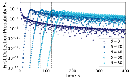
Figure 1: $F_{n}$ vs. $n$ for different $\delta$, with $\tau=0.25$ ($\gamma=1$ as mentioned). The dashed lines represent the $n_{\text{inc}}=\delta/2\tau$, close to the $\max(F_{n})$. For a thorough discussion on the quantum first hitting probability, see Ref. Thiel et al. (2018a).

To determine the time when the particle arrives at some target for the first time, one cannot simply observe the “walking” process of a quantum particle, since according to Born’s rule it “freezes” the particle at some eigenstate of the observable. This gives rise to a fundamental process and debatable problem known as time-of-arrival (TOA) in quantum physics Muga and Leavens (2000). A way to solve this issue renders the framework of “monitoring” the (unitary) walking process built to define the quantum first detected passage time or first hitting time, via some measurement protocol, within which the stroboscopic measurement protocol has been investigated in full detail Krovi and Brun (2006); Grünbaum et al. (2013); Dhar et al. (2015a, b); Friedman et al. (2017); Thiel et al. (2018a, b); Yin et al. (2019); Liu et al. (2020); Tornow and Ziegler (2022). The stroboscopic monitoring protocol states the following: a quantum walker is initially dispatched at a localized state $\ket{x_{\text{0}}}$ (source), and one attempts to measure the walker on the detected state $\ket{x_{\text{d}}}$ (target) at fixed times, $(\tau,2\tau,3\tau,\cdots)$. In between the measurement attempts, the system undergoes free evolution dictated by the Schrödinger equation. We employ von Neumann (strong) measurement described by the projection $\hat{D}=\ket{x_{\text{d}}}\bra{x_{\text{d}}}$, so the outcome of each measurement is yes (detection) or no (null detection) with probabilities determined by the Born rule. For the first hitting of the walker at the $n$th measurement attempt, the output of the experiment must be “no, no, no, no, …, yes”, namely a final success at the $n$th attempt following previous $n-1$ failure, since the experiment is done once the walker hits the detector, i.e., a yes event is recorded. Each null detection acts as a wipe-out of the component of the wave function at the target Grünbaum et al. (2013); Dhar et al. (2015b); Friedman et al. (2017). We will explain the effects from the null detection below, which manifest themselves in the quantum renewal equation. Inherently, $n$ is a random variable, and is defined as the first detected passage time or hitting time (in units of $\tau$). We denote the amplitude of finding the walker for the first time at the $n$th attempt by $\phi_{n}$ Dhar et al. (2015b). Using the quantum renewal equation, one can in principle solve for the quantum first hitting amplitude Friedman et al. (2017):

$$\phi_{n}(x_{\text{d}},x_{0})=\bra{x_{\text{d}}}\hat{U}(n\tau)\ket{x_{0}}-\sum_{m=1}^{n-1}\bra{x_{\text{d}}}\hat{U}[(n-m)\tau]\ket{x_{\text{d}}}\phi_{m}.$$ (3)

Technically one uses Eq. (2) and iterations to solve this equation or one may employ generating function techniques. For example, $\phi_{1}=i^{|x_{\text{d}}-x_{0}|}J_{|x_{\text{d}}-x_{0}|}(2\tau)$, which is expected from basic quantum mechanics Eq. (2), while $\phi_{2}=i^{|x_{\text{d}}-x_{0}|}\left[J_{|x_{\text{d}}-x_{0}|}(4\tau)-J_{0}(2\tau)J_{|x_{\text{d}}-x_{0}|}(2\tau)\right]$. Eq. (3) is a quantum counterpart of the well-known classical renewal equation, which is discussed in Ref. Redner (2001). From Eq. (3), one can readily find the essential effects from the repeated local measurement conditioned with null outcome: the first hitting amplitude is indeed related to the measurement-free transition amplitude $\bra{x_{\text{d}}}\hat{U}(n\tau)\ket{x_{0}}$, but the measurement-free return amplitude propagated from the prior first hitting amplitude, $\bra{x_{\text{d}}}\hat{U}[(n-m)\tau]\ket{x_{\text{d}}}\phi_{m}$ ($m<n$), should be subtracted, since they represent the events that have been aborted by the null detection from the statistical ensemble.

Using Eq. (3), one then finds $F_{n}$, the first hitting probability at time $n$,

$$F_{n}=|\phi_{n}|^{2}.$$ (4)

With Eq. (2) and $\delta:=|x_{\text{d}}-x_{\text{0}}|$, that denotes the distance between the source and target in units of the lattice constant, one obtains, via iterations Friedman et al. (2017):

$$F_{1} =|\phi_{1}|^{2}=J^{2}_{\delta}(2\tau),$$ (5)

$$F_{2} =[J_{\delta}(4\tau)-J_{0}(2\tau)J_{\delta}(2\tau)]^{2},$$

$$F_{3} =[J_{\delta}(6\tau)-J_{0}(4\tau)J_{\delta}(2\tau)-J_{0}(2\tau)J_{\delta}(4\tau)+J^{2}_{0}(2\tau)J_{\delta}(2\tau)]^{2},$$

$$\;\;\vdots$$

A numerical demonstration is presented in Fig. 1 for different values of $\delta$. As one may witness in the figure, besides the oscillatory decays, the maximum of $F_{n}$ plays the role of a transition point distinguishing a rapid growth and a slow decay of $F_{n}$. The dashed lines at $n=40,80,120,160$ (correspond to $\delta=20,40,60,80$) approximately point to the maxima, and those special values of $n$ are given by the maximal group velocity $\max(v_{g})=\max\left[|\partial_{k}E(k)|\right]=2$, the distance $\delta$, and the measurement period $\tau$ in a kinematic fashion: $n_{\text{inc}}:=\delta/2\tau$, hence we regard it as the “incidence” time of the ballistic-propagating wave-front Thiel et al. (2018a). Around the $n_{\text{inc}}$, the chance for the detector to be hit reaches the maximum. Detailed analysis of $F_{n}$ is provided in Friedman et al. (2017); Thiel et al. (2018a). For a classical random walk, roughly speaking one has a peak in $F_{n}$ that is determined by diffusive motion and the initial distance of target and source, followed by a power-law decay. In the quantum world non-trivial oscillations determined by a phase, superimpose on power-law decay are found Thiel et al. (2018a). Yet another difference between the classical and quantum hitting time problem is that the former is recurrent, while the latter is not, namely in general $\sum_{n=1}^{\infty}F_{n}<1$ in the quantum case Krovi and Brun (2006); Thiel et al. (2020a, b).

Now we will incorporate the restart framework with the quantum hitting time. As shown before, the ballistic propagation is a quantum advantage in faster search (over classical diffusive motion), however, as mentioned, $F_{n}$ is unfortunately non-normalized in this $1$D model (also in many finite systems), leading to infinite mean fitting times Krovi and Brun (2006). This indicates that the probabilistic nature of quantum dynamics sends the walker to undesired “trajectories” far away from the target, or to the states orthogonal to the detected state in the Hilbert space forever Thiel et al. (2020b). A systematic strategy to solve this problem, inspired from processes happening in nature Munsky et al. (2009); Bel et al. (2009); Rotbart et al. (2015) or algorithmic methods used in classical computers Gomes et al. (1998a, b), is to perform restarts to rescue a process that probably enters a wrong track. We expect the approach of restart to take advantage of the ballistic spreading of the wave-front in each single run (one run is a monitored process between restarts), and in the mean time, to guarantee the detection of the quantum walker (see Appendix A), so that the quantum advantage of faster search is reinforced to pronounce the supremacy of the quantum search.

III The first hitting statistics under restart

We will consider the deterministic restart (or sharp restart) strategy, namely, after every $r$ failed attempts in detecting the particle, the system is reset to the initial state to restart the monitored process. This strategy has been proven as the outperforming one, in the sense of unfailingly achieving the lowest minimum of the mean hitting time among all random restart strategies Luby et al. (1993); Pal and Reuveni (2017). Let $n_{R}$ be the first hitting time under restart in units of $\tau$. The general formula for the mean hitting time under sharp restart $\expectationvalue{n_{R}(r)}$ (the variable $r$ means $r$ steps between restarts) is

$$\expectationvalue{n_{R}(r)}=r{1-P_{\rm det}^{r}\over P_{\rm det}^{r}}+\expectationvalue{n}^{r}_{\text{cond}},$$ (6)

where $P_{\rm det}^{r}:=\sum_{n=1}^{r}F_{n}$ is the detection probability within $r$ attempts, and $\expectationvalue{n}^{r}_{\text{cond}}:=\sum_{n=1}^{r}nF_{n}/P_{\rm det}^{r}$ is the conditional mean of the first hitting provided the particle is detected within $r$ attempts. The $F_{n}$ are the restart-free probabilities given with Eq. (5). This result has been presented in Refs. Luby et al. (1993); Bonomo and Pal (2021), and we also provide an alternative derivation in Appendix B. We note that in the large $r$ limit, for classical random walks in dimension one, $P_{\rm det}^{r}\to 1$, then $\expectationvalue{n_{R}(r)}\to\expectationvalue{n}^{r}_{\text{cond}}$, while for the quantum walk Eq. (1), as mentioned above, $P_{\rm det}^{r}\to\sum_{n=1}^{\infty}F_{n}<1$. This implies that the first term in the right-hand side of Eq. (6), $r(1-P_{\rm det}^{r})/P_{\rm det}^{r}$, cannot be neglected in the large $r$ limit. We will show later that for the quantum walk on an infinite line, $\expectationvalue{n_{R}(r)}\sim ar+b$ when $r\to\infty$, with $a=(1-P_{\rm det}^{r=\infty})/P_{\rm det}^{r=\infty}$, $b=\expectationvalue{n}^{r=\infty}_{\text{cond}}$, namely, $\expectationvalue{n}^{r}_{\text{cond}}$ in the quantum case converges to a finite number.

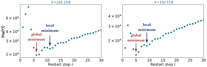
Figure 2: $\expectationvalue{n_{R}(r)}$ vs. $r$ for $\delta=60$, with different $\tau$. We see the oscillations of $\expectationvalue{n_{R}(r)}$ render the presence of several extrema (see the arrows), and the global minimum is located in small $r$, which will be analyzed below. When $\tau$ changes from $150.10\pi$ to $150.12\pi$, we see a big change in the minimum of $\expectationvalue{n_{R}(r)}$, namely $\min{\expectationvalue{n_{R}(r)}}=19615\to 13287$, with the optimal restart step changing from $6$ to $5$. This shows that a slight change of $\tau$ causes a very large change of the optimum, indicating a type of instability.

In principle, substituting the first hitting probability $F_{n}$ Eq. (5) into the formula for the mean detection time under restart Eq. (6), we obtain $\expectationvalue{n_{R}(r)}$ for this specific model, an approach that is used to test the approximations studied below, the latter providing insights into the behaviors of the quantum restart. We provide a numerical demonstration of the general landscape of $\expectationvalue{n_{R}(r)}$ in Fig. 2. The first remarkable feature is the oscillations of $\expectationvalue{n_{R}(r)}$, leading to multiple extrema, which is vastly different from the classical restart with one distinct minimum Gupta and Jayannavar (2022). Second, we notice that a small variation of the sampling time $\tau$ leads to a large change of the optimum, which switches in this example from $\expectationvalue{n_{R}(6)}=19615$ to $\expectationvalue{n_{R}(5)}=13287$. This suggests a type of instability as mentioned in the introduction. Note the measurement periods $\tau$’s are chosen large here ($\tau=150.10\pi,\,150.12\pi$), which allows the application of asymptotic methods on our problem soon to be discussed.

More precisely, we list a few analytical expressions for $\expectationvalue{n_{R}(r)}$ using Eqs. (3,5,6),

$$\expectationvalue{n_{R}(1)} ={1\over F_{1}}={1\over J^{2}_{\delta}(2\tau)},\quad\quad\quad\,\,\,$$ (7)

$$\expectationvalue{n_{R}(2)} ={2-F_{1}\over F_{1}+F_{2}}={2-J^{2}_{\delta}(2\tau)\over J^{2}_{\delta}(2\tau)+[J_{\delta}(4\tau)-J_{0}(2\tau)J_{\delta}(2\tau)]^{2}},$$

$$\expectationvalue{n_{R}(3)} ={3-2F_{1}-F_{2}\over F_{1}+F_{2}+F_{3}}={3-2J^{2}_{\delta}(2\tau)-[J_{\delta}(4\tau)-J_{0}(2\tau)J_{\delta}(2\tau)]^{2}\over F_{1}+F_{2}+F_{3}},$$

$$\expectationvalue{n_{R}(4)} ={4-3F_{1}-2F_{2}-F_{3}\over F_{1}+F_{2}+F_{3}+F_{4}},\;\;\expectationvalue{n_{R}(5)}={5-4F_{1}-3F_{2}-2F_{3}-F_{4}\over F_{1}+F_{2}+F_{3}+F_{4}+F_{5}},\;\;\cdots$$

Those expressions are cumbersome, however we will analyze particular limits where we may provide insights, e.g. large measurement period $\tau$. In what follows, our discussions will be based on choosing certain values for $\delta$ to gain some insights (e.g., $\delta=0,1,2,\cdots$), and investigating how to optimize the mean hitting time under restart. One of our goals is to find the optimal restart time $r$, denoted by $r^{*}$, which will be in general a function of $\tau$ and $\delta$. The corresponding $\expectationvalue{n_{R}(r^{*})}$ is then the optimal in the mean sense.

IV Optimization of the mean hitting time

IV.1 Return case: $\delta=0$

We start with the “return” case where the detector is put at the origin to monitor the walker’s first return, namely, $\delta=0$ Friedman et al. (2017). We first consider the Zeno limit $\tau\to 0$. Specially, in this limit, we have the following asymptotics for $\expectationvalue{n_{R}(r)}$ using Eq. (7):

$$\expectationvalue{n_{R}(1)}\sim 1+2\tau^{2},\;\;\;\expectationvalue{n_{R}(2)}\sim 1+4\tau^{2},\;\;\;\expectationvalue{n_{R}(3)}\sim 1+6\tau^{2},\cdots$$ (8)

Clearly, the minimum is $\expectationvalue{n_{R}(1)}$. Hence the optimal restart $r^{*}=1$ in the Zeno regime, and this is also intuitive, since the wave function is nearly frozen at the origin in the Zeno limit Misra and Sudarshan (1977), and it is always the best choice to restart after each failed measurement.

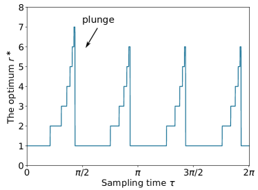
Figure 3: The optimal restart time $r^{*}$ as a function of $\tau$ for $\delta=0$. We see the staircase structure accompanied by periodical plunges (see the arrow).

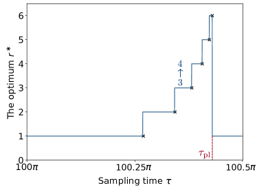
Figure 4: $r^{*}$ versus $\tau$ in the large $\tau$ limit exhibits a limiting staircase and plunge. Here we use $\tau\in[100\pi,100.5\pi]$ and $\delta=0$. The cyan lines are the exact results, and the black crosses represent the approximations using Table 1(b). $\tau_{\text{pl}}$ here is approximated as $k\pi/2+1.353$ with $k=200$.

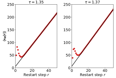
Figure 5: $\expectationvalue{n_{R}(r)}$ vs. $r$ in the vicinity of the plunge $\tau$ ($\approx 1.36$), see the drop of $r^{*}$ ($7\to 1$) at the leftmost staircase in Fig. 3. There are two minima competing with each other, and a small change of $\tau$ ($1.35\to 1.37$) results in different optima. On the left panel $r^{*}=7$ and on the right $r^{*}=1$. Thus a small change of $\tau$ creates a plunge of $r^{*}$. The solid lines represent the approximations to $\expectationvalue{n_{R}(r)}$ in large $r$ limit, i.e., $\expectationvalue{n_{R}(r)}\sim r(1-P_{\rm det}^{r=\infty})/P_{\rm det}^{r=\infty}+\expectationvalue{n_{R}(\infty)}_{\text{cond}}$, where $\expectationvalue{n_{R}(\infty)}_{\text{cond}}=\sum^{\infty}_{n=1}nF_{n}/\sum^{\infty}_{n=1}F_{n}$.

For large $\tau$, with the large $x$ asymptotics for $J_{n}(x)$, namely, $J_{n}(x)\sim\sqrt{2/\pi x}\cos(x-\pi n/2-\pi/4)$ Gradshteyn and Ryzhik (2007), we can re-express $F_{n}$ for finite $n$ as Friedman et al. (2017)

$$F_{n}(\tau)\sim{1\over n\pi\tau}\cos^{2}\left(2n\tau-{\pi\over 4}\right).$$ (9)

In this limit there is a simple relation between the probability of first hitting time and the measurement-free wave function. Namely, $F_{n}\sim P(0,0,t)=|\bra{0}\ket{\psi(t)}|^{2}=J_{0}^{2}(2t)$ with $t=n\tau$ and $\ket{\psi(t)}$ is the solution of the Schrödinger equation, in the absence of measurement, see Eq. (2). If $2\tau$ is a multiple of $\pi$, we find using Eq. (9)

$$F_{n}\sim{1\over 2n\pi\tau}.$$ (10)

Thus, the restart-free $F_{n}$ decays monotonically with $n$. For such a case, the best strategy of restart is to use $r=1$, namely, to restart after each measurement. We then have

$$r^{*}=1,\quad\text{when}\,\,\,2\tau=k\pi,$$ (11)

where $k$ is an integer. Using Eqs. (7,10), $\expectationvalue{n_{R}(r^{*})}\sim 2\pi\tau$.

We now study how this optimal restart changes when we vary the sampling time $\tau$, in particular, what is $r^{*}$ as a function of $\tau$? We have found that $r^{*}$ exhibits a set of staircases, see Fig. 3. Clearly this behavior is far from the classical limit, and it is due to the oscillations of the first hitting probability $F_{n}$. The optimal choice of $r$, presented in Fig. 3, is a periodical function of $\tau$, with a period of $\pi/2$. Starting with $\tau=\pi k/2\gg 1$, where $k$ is an integer, when we increase $\tau$ slightly beyond this critical point, we find that $\expectationvalue{n_{R}(1)}$ is the optimal, i.e., the fastest approach to restart is still $r^{*}=1$. We see transitions as $\tau$ is varied, from $r^{*}=1$ to $r^{*}=2$, and then to $r^{*}=3$, etc., and finally a plunge to $r^{*}=1$, and this is repeated. The staircase for small $\tau$ is not identical to that for large $\tau$, however, as to be shown below in the latter limit, we will reach a particular pattern of staircases, presented in Fig. 4.

Now we also use the fact that $F_{n}\ll 1$ in the limit under study, namely the large $\tau$ limit. Using Eq. (7), we find that the condition for $\tau$, for the $r^{*}=1$ to $r^{*}=2$ transition, i.e., $\expectationvalue{n_{R}(1)}=\expectationvalue{n_{R}(2)}$, reads

$$F_{1}(\tau)=F_{2}(\tau),$$ (12)

and $F_{n}$ are given in Eq. (9). We then find a sequence of transitions, and due to the fact that $F_{n}$ is small, we find using Eq. (7), the transition $r^{*}=2\to r^{*}=3$ at $\tau$ which solves

$$F_{3}(\tau)=[F_{1}(\tau)+F_{2}(\tau)]/2,$$ (13)

and similarly for the $r^{*}=3\to r^{*}=4$ transition shown in Fig. 4,

$$F_{4}(\tau)=[F_{1}(\tau)+F_{2}(\tau)+F_{3}(\tau)]/3.$$ (14)

We see that the transitions are taking place when $F_{n}$ is the mean of all the proceeding $F_{i}$’s. At some stage these equations cannot be solved, in the sense that there is no $\tau$ giving a valid solution. We encountered already such a situation, and that is the Zeno limit. We can use Eq. (9) for $F_{n}(\tau)$ and find, with a simple computer program of calculation, the transitions in $r^{*}$ at special sampling times.

Note that we have plunges where $r^{*}$ falls to the value $1$ (see the arrow in Fig. 3). In Fig. 5, we choose as an example two values of $\tau$ in the vicinity of $\tau\approx 1.36$. At this value we have a plunge (see Fig. 3). As shown in Fig. 5, there are two minima competing with each other, and the global minimum switches between them when $\tau$ is slightly varied. At the exact transition time $\tau$ for the plunge, the two minima are identical. Thus the system exhibits an instability in the sense that small changes of $\tau$ create large difference in the optimal restart time $r^{*}$.

We now calculate the sampling time $\tau_{\text{pl}}$, where plunges are found. Let $\tau=k\pi/2+\epsilon$ and $0<\epsilon<\pi/2$. As mentioned in Eq. (11), if $\epsilon=0$, $r^{*}=1$. We then denote $\epsilon_{1\to 2}$ as the value of $\epsilon$ where we have a transition from $r^{*}=1$ to $r^{*}=2$, similarly for other transitions. In between the transition $\epsilon$, namely for each interval $[\epsilon_{k\to k+1},\epsilon_{k+1\to k+2}]$, we will check whether $\expectationvalue{n_{R}(k+1)}$ remains the minimum, and especially compare it with $\expectationvalue{n_{R}(1)}$ in case we miss the plunge to $r^{*}=1$. With Eq. (9) and Eqs. (12-14) we get Table 1(b) which gives the values or $\epsilon$ for the various transitions, and check the minimum in Table 1(b).

Table 1: The $\epsilon$ at the transitions of $r^{*}$ for $\delta=0$.

(a) The values of $\epsilon_{k\to k+1}$.

$\epsilon_{k\to k+1}$	$\epsilon_{1\to 2}$	$\epsilon_{2\to 3}$	$\epsilon_{3\to 4}$	$\epsilon_{4\to 5}$	$\epsilon_{5\to 6}$	$\epsilon_{\text{pl}}$
Value	0.850	1.081	1.204	1.280	1.332	1.353

(b) The relation between $\expectationvalue{n_{R}(k)}$ and $\expectationvalue{n_{R}(1)}$ in $[\epsilon_{k-1\to k},\epsilon_{k\to k+1}]$.

$[\epsilon_{1\to 2},\epsilon_{2\to 3}]$	$[\epsilon_{2\to 3},\epsilon_{3\to 4}]$	$[\epsilon_{3\to 4},\epsilon_{4\to 5}]$	$[\epsilon_{4\to 5},\epsilon_{5\to 6}]$	$[\epsilon_{5\to 6},\epsilon_{\text{pl}}]$	$[\epsilon_{\text{pl}},\pi/2]$
$\expectationvalue{n_{R}(2)}<\expectationvalue{n_{R}(1)}$	$\expectationvalue{n_{R}(3)}<\expectationvalue{n_{R}(1)}$	$\expectationvalue{n_{R}(4)}<\expectationvalue{n_{R}(1)}$	$\expectationvalue{n_{R}(5)}<\expectationvalue{n_{R}(1)}$	$\expectationvalue{n_{R}(6)}<\expectationvalue{n_{R}(1)}$	$\expectationvalue{n_{R}(1)}<\expectationvalue{n_{R}(6)}$

Note that for the transitions with large $r^{*}$, $\epsilon$ is accumulating close to $\pi/2$, and hence the plateaus in optimal $r$ are very small. Furthermore, when $1.353<\epsilon<\pi/2$, $r^{*}$ drops to $1$, i.e., a sudden plunge as mentioned. So we have

$$\tau_{\text{pl}}=1.353+\pi k/2$$ (15)

for large $k$, and in other words, let $\tau_{\text{pl}}=\pi k/2+\epsilon_{\text{pl}}$, then $\epsilon_{\text{pl}}=1.353$. As shown in Fig. 3, $r^{*}$ is plotted versus $\tau$, and we see staircases, where $r^{*}$ is increasing by unit steps, as our theory predicts, and then a sudden plunge. The staircase structure and plunges of $r^{*}$ versus $\tau$ are found in the whole range of $\tau$, and are not limited to large $\tau$ limit studied presented analytically in Table 1(b).

A general formalism to obtain the transition $\epsilon$ is stated as follows. We find using $F_{n}\ll 1$ valid from the large $\tau$ limit and Eq. (6),

$$\expectationvalue{n_{R}(r)}\sim r\big{/}\sum_{n=1}^{r}F_{n}.$$ (16)

Then the condition for the transition $\tau$ that leads to $\expectationvalue{n_{R}(r)}=\expectationvalue{n_{R}(r+1)}$ reads

$$F_{r+1}=\sum^{r}_{n=1}F_{n}/r.$$ (17)

With $P_{\text{det}}^{r}=\sum^{r}_{n=1}F_{n}$, the transcendental equation Eq. (17) becomes

$$P_{\text{det}}^{r}(\epsilon)=rF_{r+1}(\epsilon),$$ (18)

which yields a set of values of $\tau$ and $r$, and as noted above this gives $\expectationvalue{n_{R}(r)}=\expectationvalue{n_{R}(r+1)}$. Now exploiting the fact that the values of $r^{*}$ have a staircase structure, we start with $\epsilon=0$, and then $r^{*}=1$, increasing $\epsilon$, we get the transition point $r^{*}=1\to r^{*}=2$, denoted by $1\to 2$ transition. We then continue increasing $\epsilon$ to find the transition $2\to 3$, etc. This means that the above formula yields the values of $r^{*}$ at sampling times given by $\epsilon$. This is a valid approximation in the case of large $\tau$ only as mentioned, and in this case, with Eq. (9) we have to solve for

$$\sum_{n=1}^{r}{1\over n}\cos^{2}\left(2n\epsilon-{\pi\over 4}\right)={r\over r+1}\cos^{2}\left[2(r+1)\epsilon-{\pi\over 4}\right],$$ (19)

and again we must increase $\epsilon$ from zero using $r=1$, to find the first transition $r^{*}=1\to r^{*}=2$ at $\epsilon_{1\to 2}$, then update to $r=2$ finding the transition point $\epsilon_{2\to 3}$ etc. It is clear that when $r$ is very large, there is no solution to Eq. (19). Since the left-hand side of Eq. (19) can be simplified as $(1/2)\sum^{r}_{n=1}[1/n+\sin(4n\epsilon)/n]$, and in large $r$ limit, $\sum^{r}\sin(4n\epsilon)/n\to(\pi-4\epsilon)/2$, and $\sum^{r}1/n\to\infty$ does not converge, while the right-hand side is always bounded by $1$. Physically it makes sense that we cannot witness the transitions forever, since as mentioned $\expectationvalue{n_{R}(r)}$ is proportional to $r$ in large $r$ limit, there must exist a minimum at finite $r$. We cannot expect a restart strategy to be useful for $r\gg 1$. See Fig. 4 for the comparison between exact results and approximations [Eq. (19), Table 1(b)].

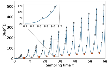
Figure 6: The optimal mean $\expectationvalue{n_{R}(r^{*})}$ vs. $\tau$ for $\delta=0$ (cyan curve). The black crosses representing $\expectationvalue{n_{R}(r^{*})}$ at transition $\tau$’s are plotted using Eq. (22). And at those transitions, nonsmoothness $\expectationvalue{n_{R}(r^{*})}$ is witnessed (see the inset). The minima of $\expectationvalue{n_{R}(r^{*})}$ are predicted by Eq. (23) and presented by red closed circles. As shown in the figure, $\expectationvalue{n_{R}(r^{*})}$ exhibits large fluctuations and periodic-like behavior when the sampling time $\tau$ is varied. The peaks of $\expectationvalue{n_{R}(r^{*})}$ are found close to the plunges of $r^{*}$ shown in Fig. 3, namely close to the instability points like the one presented in Fig. 5. See more details about the plot in Appendix C. For an efficient search one clearly needs to consider the optimization of the process both with respect to the restart time, but also with respect to the sampling period $\tau$.

After finding the optimal $r^{*}$, we study the mean $\expectationvalue{n_{R}(r^{*})}$, at the optimal choice $r^{*}$, which is of course the fastest way in mean sense to detect the particle. Note that when $F_{n}\ll 1$, using Eq. (16), we have

$$\expectationvalue{n_{R}(r^{*})}\sim{r^{*}\over\sum^{r^{*}}F_{n}}.$$ (20)

From above arguments Eq. (17), at those transition $\tau$, we have

$$\expectationvalue{n_{R}(r^{*})}\sim{1\over F_{r^{*}+1}}.$$ (21)

This is obtained by calculating $F_{n}$, at the corresponding $\epsilon$, namely, using Eq. (9),

$$\expectationvalue{n_{R}(r^{*})}\sim{(r^{*}+1)\pi\tau\over\cos^{2}[2(r^{*}+1)\tau-\pi/4]}.$$ (22)

See Fig. 6 for the numerical confirmation. The exact results are represented by the cyan line. And the theoretical $\expectationvalue{n_{R}(r^{*})}$ at transition $\tau$’s calculated by Eq. (22) are represented by black crosses, at which nonsmoothness of $\expectationvalue{n_{R}(r^{*})}$ appears. As $\tau$ is increased, the general trend is an increase of $\expectationvalue{n_{R}(r^{*})}$, which is expected since the wave packet for large $\tau$ has spread out far from the detector when $\delta=0$. In addition to this trend we have a periodical set of maxima. Note the dramatic changes in those maxima presented in the figure. The maxima are at the plunge $\tau$’s, where $r^{*}$ falls from $6$ to $1$. The minima of $\expectationvalue{n_{R}(r^{*})}$ are actually the minima of $\expectationvalue{n_{R}(1)}=1/F_{1}$, or the maxima of $F_{1}$. In large $\tau$ limit, using Eq. (9), we find when $\tau=\pi/8+k\pi/2$, $\max(F_{1})=(\pi^{2}/8+k\pi^{2}/2)^{-1}$, then the minima of $\expectationvalue{n_{R}(r^{*})}$ is

$$\min(\expectationvalue{n_{R}(r^{*})})={1\over\max(F_{1})}={\pi^{2}\over 8}+k{\pi^{2}\over 2}.$$ (23)

We plot in closed circles these theoretical minima indicated by Eq. (23). Our theory Eqs. (22,23) nicely matches the numerics, as shown in Fig. 6.

IV.2 $\delta=1$

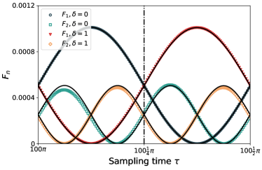
Figure 7: $F_{n}$ vs. $\tau\in[100\pi,100{1\over 2}\pi]$ for $n=1,2$ and $\delta=0,1$. The black curves represent the trigonometric approximations Eqs. (9,26). As shown and mentioned in texts, the $F_{n}$’s for $\delta=1$, in each interval $[\pi k/2,\pi(k+1)/2]$, are symmetric to the ones for $\delta=0$ about $\pi k/2+\pi/4$ (the dashed line).

Here we investigate the case where the detector is put at the neighboring site to the origin, namely $\delta=1$. In the Zeno regime, namely $\tau\to 0$, using Eq. (7), we have

$$\expectationvalue{n_{R}(1)}\sim 1+\tau^{-2},\;\;\;\expectationvalue{n_{R}(2)}\sim{5\over 2}+\tau^{-2},\;\;\;\expectationvalue{n_{R}(3)}\sim{14\over 3}+\tau^{-2},\cdots$$ (24)

Hence $r^{*}=1$ when $\tau\to 0$. The physical picture is the following: for small $\tau$ we have a leakage of amplitude, from the starting point $x=0$, both to $x=1$ and to $x=-1$, in fact the amplitudes at these states are the same. Now one tries to detect on $x=1$, and does not find the particle. One may choose to restart, which means that the amplitude at $x=-1$ restores to $x=0$. This benefits detection. If looking at the asymptotics of the first hitting probability, with Eq. (5), we find in the limit $\tau\to 0$,

$$F_{1}\sim\tau^{2}-\tau^{4},\;\;\;F_{2}\sim\tau^{2}-5\tau^{4},\;\;\;F_{3}\sim\tau^{2}-11\tau^{4},\cdots$$ (25)

So $F_{1}>F_{2}>F_{3}>\cdots$, indicating that continuing with the measurement is not beneficial and a restart is the best option to speed up search. Hence performing restart after each failed measurement is the best strategy, and $r^{*}=1$ when $\tau\to 0$.

In the opposite limit of large $\tau$, we have

$$F_{n}\sim{1\over n\pi\tau}\cos^{2}\left(2n\tau-{3\pi\over 4}\right).$$ (26)

For $\tau=\pi k/2$, we find again that $F_{n}\sim(2n\pi\tau)^{-1}$, and $r^{*}=1$, the same as Eqs. (10, 11). To be more specific, since $F_{n}$ is a monotonic decaying function, for these special values of $\tau$ the best strategy is to restart after the first measurement. Similar to the case $\delta=0$, we expect that increasing $\tau$ in every interval $[\pi k/2,\pi(k+1)/2]$ leads to the quanta jumps of $r^{*}$. While it is noteworthy that if we let $\tau=\pi k/2-\epsilon$ with $k\gg 1$, Eq. (26) becomes

$$F_{n}\sim{1\over n\pi\tau}\cos^{2}\left(-2n\epsilon-{3\pi\over 4}\right)={1\over n\pi\tau}\cos^{2}\left(2n\epsilon-{\pi\over 4}\right),$$ (27)

which recovers to the case $\delta=0$. This means that in the range $\tau\in[\pi k/2,\pi(k+1)/2]$, $F_{n}$ in the case of $\delta=1$ is symmetric to that in the case of $\delta=0$, with respect to $\tau=\pi k/2+\pi/4$, when $k$ is large, as shown in Fig. 7. Therefore, we expect the behaviors of $r^{*}$ in the case $\delta=1$ is a mirror reflection to that in the case $\delta=0$ in every interval $[\pi k/2,\pi(k+1)/2]$, with the symmetry axis at $\pi k/2+\pi/4$. Then the transition $\epsilon$’s are associated via $\epsilon\leftrightarrow\pi/2-\epsilon$ when $\delta$ switches between $0$ and $1$. In Fig. 8 we plot $r^{*}(\tau)$ with $\tau\in[0,2\pi]$, and the staircase structure is symmetric to the previous case, even when $\tau$ is not large. In large $\tau$ limit, there appears definite symmetry (as seen in Fig. 9).

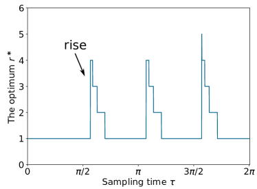
Figure 8: The optimal restart time $r^{*}$ as a function of $\tau$ for $\delta=1$. We see the staircase structure along with periodical rises, i.e., $r^{*}$ jumping from $1$ to $4$ or $5$ (see the arrow). The series of plateaus declines from the maximum from left to right unlike the case $\delta=0$ where we find the opposite trend [see Fig. 3].

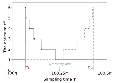
Figure 9: $r^{*}$ versus $\tau$ with $\tau\in[100\pi,100.5\pi]$ and $\delta=1$. The cyan lines are the exact results obtained using Eq. (6), and the black crosses represent the approximations [via applying $\epsilon\to\pi/2-\epsilon$ to Eq. (19)]. $\tau_{\text{r}}$ here is approximated as $k\pi/2+0.218$ with $k=200$. This is a mirror image of Fig. 4 (the gray dashed line here), so the parity of the initial condition determines the staircase structure which otherwise is universal in the sense that it does not depend on the initial condition. The symmetry axis for the two staircase patterns is $k\pi/2+\pi/4$ with $k=200$ here.

A calculation similar to that in Table 1(b) is provided in Appendix D. And in the case $\delta=1$ we have a sudden rise in $r^{*}$, unlike the plunge for $\delta=0$. The rise $\tau$, denoted by $\tau_{\text{r}}$, is equal to $\pi/2-\epsilon_{\text{pl}}\approx 0.218$. And those transition $\epsilon$ are all symmetric to that in the case $\delta=0$ about $\pi/4$, as expected. See Fig. 9 for a comparison between the exact results and approximations.

Furthermore, one can readily show that in the case of even or odd $\delta$, Eq. (9) or Eq. (26) always hold, respectively, and the pattern presented in Fig. 9 is generic. This insightfully indicates the $\delta$-independence of $F_{n}$ for all even/odd $\delta$, in large sampling time limit (similar properties are shown in Ref. Thiel et al. (2018a)). In other words, large $\tau$ renders $F_{n}$’s dependence only on the parity of distance between the initial and detected sites. We will see this more clearly after the discussion on $\delta=2$.

IV.3 $\delta=2$

When $\delta=2$, in the limit of $\tau\to 0$, we find using Eq. (5)

$$F_{1}\sim{1\over 4}\tau^{4}-{1\over 6}\tau^{6},\;\;\;F_{2}\sim{9\over 4}\tau^{4}-6\tau^{6},\;\;\;F_{3}\sim{25\over 4}\tau^{4}-{235\over 6}\tau^{6},\cdots$$ (28)

Namely $F_{1}<F_{2}<F_{3}<\cdots$ till some $n\sim 1/\tau$ and then decreases. This behavior is very different if compared with the cases $\delta=0$ and $\delta=1$, where $F_{1}$ was the maximum of the set $\{F_{1},F_{2},F_{3},...\}$. We expect that $r^{*}$ exhibits divergence in this limit, see Fig. 10. Checking the asymptotics of $\expectationvalue{n_{R}(r)}$, with Eq. (7), we have

$$\expectationvalue{n_{R}(1)}\sim 4\tau^{-4},\;\;\;\expectationvalue{n_{R}(2)}\sim{4\over 5}\tau^{-4},\;\;\;\expectationvalue{n_{R}(3)}\sim{12\over 35}\tau^{-4},\cdots$$ (29)

Hence $\expectationvalue{n_{R}(1)}>\expectationvalue{n_{R}(2)}>\expectationvalue{n_{R}(3)}>\cdots$. We use the theory in Ref. Yin and Barkai (2022), to study the Zeno limit.

Assuming large $\tau$, $F_{n}$ is re-expressed as Friedman et al. (2017); Thiel et al. (2018a)

$$F_{n}\sim{1\over n\pi\tau}\cos^{2}\left(2n\tau-{\pi\over 4}\right).$$ (30)

This is the same as in the case $\delta=0$, since the initial condition $\delta$ only affects the phase in $F_{n}$ via $\pi\delta/2$, and then the same parity of $\delta$ leads to the same $F_{n}$, and to the same pattern of $r^{*}(\tau)$. Thus we could use Table 1(b) to approximate $r^{*}$’s staircase structure in this case, see Fig. 11.

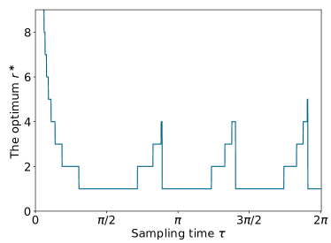
Figure 10: The optimal restart time $r^{*}$ as a function of $\tau$ for $\delta=2$. We see the staircase structure along with periodical plunges.

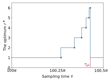
Figure 11: $r^{*}$ versus $\tau$ with $\tau\in[100\pi,100.5\pi]$ and $\delta=2$. The cyan lines are the exact results, and the black crosses represent the approximations using Table 1(b). $\tau_{\text{pl}}$ here is approximated as $100\pi+1.353$.

IV.4 The parity of $\delta$ matters

Following above discussion, we note a remarkable feature of the quantum first hitting times probabilities, namely that beyond a phase, they are independent of $\delta$:

$$\text{For Even $\delta$:}\quad F_{n} \sim{1\over n\pi\tau}\cos^{2}\left(2n\tau-{\pi\over 4}\right),$$ (31)

$$\text{For Odd $\delta$:}\quad F_{n} \sim{1\over n\pi\tau}\cos^{2}\left(2n\tau-{3\pi\over 4}\right).$$

This is obtained with the large argument asymptotics for $J_{n}(x)$, which was also used in the case of return in Ref. Friedman et al. (2017), and in the supplemental material of Ref. Thiel et al. (2018a). Eq. (31) is valid in the large $\tau$ limit, and we note that when $n$ is large, the first detection probability $F_{n}$ transits to a $n^{-3}$ power-law decay Friedman et al. (2017); Thiel et al. (2018a), but this does not affect our theory, which only focuses on finite $r$ restart.

Hence, based on Eq. (31), the staircase patterns, are binary and merely determined by the parity of $\delta$. These two patterns are mirror reflection to each other, connected by the operation/mapping $\epsilon_{k+1\to k}\leftrightarrow\pi/2-\epsilon_{k\to k+1}$. The origin of universality of staircase, is related to the fact that for large $\tau$, the first detection amplitude is directly associated to the wave function of the measurement-free process. This then leads to specific phases in the asymptotic expansion Eq. (31) which depends on the parity only.

To put it differently, a unity change of the distance between the target and source $\delta$, in units of the lattice constant, results in a “flipping” of the staircase pattern of the optimal restart time, which again indicates, in our view, a type of instability. This effect was demonstrated in Figs. 4,9,11.

V Summary

With restarts introduced to quantum hitting times, we find novel features that expose the instability existing in the optimization of the mean hitting time. The first feature is the presence of several minima of the mean hitting time, rather than one unique minima, as in the classical case Gupta and Jayannavar (2022). This is due to the interference-induced quantum oscillations, indicated by the Bessel function $J_{n}(x)$ in Eq. (2) and the graphic illustration in Fig. 1. These oscillations are found features of the solution to the Schrödinger equation, and the quantum first hitting time probability $F_{n}$ in the absence of restarts. These are general aspects of quantum dynamics, so we expect that our results will have a wider application than the model presented here.

Then the challenge is to find the optimum of the mean hitting time under restart. Assuming large $\tau$ (in units $\gamma=1$) for simplicity, we showed that $r^{*}(\tau)$ possesses a staircase structure of period $\pi/2$, accompanied by plunges/rises. Furthermore, there are two symmetric patterns of staircases, determined by the parity of the distance between the initial and detected sites (in units of the lattice constant). All those findings depict the instability existing in the quantum restart problems. Namely, slight changes of $\tau$ lead to a large change of $\expectationvalue{n_{R}(r)}$ (Fig. 2), optimum switching between different minima (Fig. 5), and change of the parity of $\delta$ causes a “flipping” of the staircase pattern of the optimal restart time. We want to note that the instability is not limited in the large $\tau$ case, and it is also found for small $\tau$ though then the staircases do not converge to an asymptotic limit, see the small $\tau$ limit of Fig. 3. Since the instability is essentially attributed to the oscillatory nature of the hitting time statistics, we expect its generality when changing other control parameters.

Can we foresee quantum experiments checking the validity of this work? A good platform for that aim are quantum computers, on which on-demand qubit resets have been achieved with the initial purpose of optimizing quantum circuits. The quantum walk dynamics can be mapped to a spin model through the Jordan-Wigner transformation Jordan and Wigner (1928), with repeated measurements implemented by the built-in single-qubit measurements Tornow and Ziegler (2022). Hence we feel confident that our approach can be tested in the lab.

In this work we considered a quantum walk on the line, however this is not an essential ingredient of our results, in the sense that quantum instabilities for the restart problem can be found also for finite systems. We also note that possibly other oscillatory dynamics, beyond the quantum case, will exhibit similar features to what we have found here. A key point to study the instabilities is the use of sharp restart, which as mentioned is the optimal choice. In our previous work Yin and Barkai (2022), we studied briefly quantum restarts with Poisson restarts, which did not exhibit the multiple minima found here.

Appendix A Under restart: the first hitting probability, guaranteed detection

A.1 The probability

In probability theory language, the first hitting probability $F_{n}=\text{Pr}(\overline{{\cal E}_{1}}\overline{{\cal E}_{2}}\cdots\overline{{\cal E}_{n-1}}{\cal E}_{n})$, where ${\cal E}_{k}$ denotes the event of successful detection at the $k$th attempt, and $\overline{{\cal E}_{k}}$ means the event of failing to detect the walker at the $k$th attempt. Now with the deterministic restart strategy incorporated, the new measurement protocol is as follows: after the $r$th attempt, if the walker is not yet detected, we start anew with the same initial state, until the first successful detection at the $n_{R}$th attempt with $n_{R}=r{\cal R}+\tilde{n}$, where ${\cal R}$ is the number of restart event and $\tilde{n}$ is the number of attempts till success following the last restart, and then $1\leq\tilde{n}\leq r$, ${\cal R}\geq 0$ since the restart is made just after a measurement. Following standard statistical methods, the first hitting probability under restart is:

$$F_{n_{R}}=\text{Pr}(\underbrace{\overline{{\cal E}_{1}}\cdots\overline{{\cal E}_{r}}\overline{{\cal E}_{1}}\cdots\overline{{\cal E}_{r}}}_{\text{repeat }{\cal R}\text{ times}}\overline{{\cal E}_{1}}\cdots{\cal E}_{\tilde{n}})$$ (32)

$$= \left(1-F_{1}-\cdots-F_{r}\right)^{\cal R}F_{\tilde{n}}=\left(1-\sum_{k=1}^{r}F_{k}\right)^{\cal R}F_{\tilde{n}}.$$

where $F_{j}$ are the probabilities of the first hitting at the $j$th attempt in the absence of restart. The last expression in Eq. (32) is also intuitive: the term inside the brace suggests the survival probability after $r$th measurement, the power is the number of reset event, and the term outside the brace gives the probability of first success after the last restart, thus the product of the two probability is $F_{n_{R}}$. Note here $\tilde{n}$ ranges from $1$ to $r$ (different from the remainder ranging from $0$ to $r-1$), and ${\cal R}\geq 0$. If $r=10$, $F_{n_{R}=30}$ is $\left(1-\sum_{k=1}^{10}F_{k}\right)^{2}F_{10}$.

A.2 Proof for the guaranteed detection

The restarted total detection probability $P_{\rm det}$ is

$$P_{\rm det} =\sum_{n_{R}=1}^{\infty}F_{n_{R}}=\sum_{r{\cal R}+\tilde{n}=1}^{\infty}\left(1-\sum_{j=1}^{r}F_{j}\right)^{\cal R}F_{\tilde{n}}=\sum_{{\cal R}=0}^{\infty}\sum_{\tilde{n}=1}^{r}\left(1-\sum_{j=1}^{r}F_{j}\right)^{\cal R}F_{\tilde{n}}$$ (33)

$$=\sum_{\tilde{n}=1}^{r}F_{\tilde{n}}\sum_{{\cal R}=0}^{\infty}\left(1-\sum_{j=1}^{r}F_{j}\right)^{\cal R}=\sum_{\tilde{n}=1}^{r}F_{\tilde{n}}\left(\sum_{j=1}^{r}F_{j}\right)^{-1}=1.$$

Hence the total detection probability is one provided that $\sum_{j=1}^{r}F_{j}\neq 0$, meaning that the particle will be eventually detected, as long as there exist finite probability of detection during one restart period.

Appendix B Derivation for Eq. (6) in the main text

Here we provide an alternative derivation for the mean of $n_{R}$ under restart. With Eq. (32) and the definition $\expectationvalue{n_{R}(r)}=\sum_{n_{R}=1}^{\infty}n_{R}F_{n_{R}}$, we obtain

$$\expectationvalue{n_{R}(r)}= \sum_{n_{R}=1}^{\infty}n_{R}\left(1-\sum_{k=1}^{r}F_{k}\right)^{\cal R}F_{\tilde{n}}=\sum_{r{\cal R}+\tilde{n}=1}^{\infty}\left(r{\cal R}+\tilde{n}\right)\left(1-\sum_{k=1}^{r}F_{k}\right)^{\cal R}F_{\tilde{n}}$$ (34)

$$= \sum_{{\cal R}=0}^{\infty}\sum_{\tilde{n}=1}^{r}r{\cal R}\left(1-\sum_{k=1}^{r}F_{k}\right)^{\cal R}F_{\tilde{n}}+\sum_{{\cal R}=0}^{\infty}\sum_{\tilde{n}=1}^{r}\tilde{n}\left(1-\sum_{k=1}^{r}F_{k}\right)^{\cal R}F_{\tilde{n}}$$

$$= r\sum_{\tilde{n}=1}^{r}F_{\tilde{n}}\sum_{{\cal R}=0}^{\infty}{\cal R}\left(1-\sum_{k=1}^{r}F_{k}\right)^{\cal R}+\sum_{\tilde{n}=1}^{r}\tilde{n}F_{\tilde{n}}\sum_{{\cal R}=0}^{\infty}\left(1-\sum_{k=1}^{r}F_{k}\right)^{\cal R}$$

$$= {r\left(1-\sum_{j=1}^{r}F_{j}\right)\over\sum_{j=1}^{r}F_{j}}+\underbrace{\sum_{k=1}^{r}kF_{k}\left(\sum_{k=1}^{r}F_{k}\right)^{-1}}_{\expectationvalue{n}^{r}_{\text{cond}}}=r{1-P_{\rm det}^{r}\over P_{\rm det}^{r}}+\expectationvalue{n}^{r}_{\text{cond}}.$$

This gives the Eq. (6) in the main text.

Appendix C Details in plotting Fig. 6

Since Eq. (22) is valid at the transition $\tau$, we chose $\tau=1.369+\pi k/2$ for $r^{*}=6$ with $k$ an integer [using Eq. (19)]. Although $r^{*}=6$ is cutoff by $\epsilon_{\text{pl}}=1.353$, we use the fact that $\expectationvalue{n_{R}(6)}(\tau=1.353)\approx\expectationvalue{n_{R}(6)}(\tau=1.369)=1/F_{7}(\tau=1.369)$, see Fig. 5. The black crosses nicely capture the $\expectationvalue{n_{R}(r^{*})}$ at the transition $\tau$’s.

Appendix D Transition $\tau$ in the case of $\delta=1$ and large $\tau$ limit

$$\epsilon\in[0,0.218]:\expectationvalue{n_{R}(1)}=\min(\expectationvalue{n_{R}(r)}),$$ (35)

$$\epsilon\in[0.218,\epsilon_{6\to 5}]:\expectationvalue{n_{R}(6)}<\expectationvalue{n_{R}(1)},$$

$$\epsilon_{6\to 5}=0.239=\pi/2-1.332,$$

$$\epsilon\in[\epsilon_{6\to 5},\epsilon_{5\to 4}]:\expectationvalue{n_{R}(5)}<\expectationvalue{n_{R}(1)},$$

$$\epsilon_{5\to 4}=0.291=\pi/2-1.280,$$

$$\epsilon\in[\epsilon_{5\to 4},\epsilon_{4\to 3}]:\expectationvalue{n_{R}(4)}<\expectationvalue{n_{R}(1)},$$

$$\epsilon_{4\to 3}=0.367=\pi/2-1.204,$$

$$\epsilon\in[\epsilon_{4\to 3},\epsilon_{3\to 2}]:\expectationvalue{n_{R}(3)}<\expectationvalue{n_{R}(1)},$$

$$\epsilon_{3\to 2}=0.490=\pi/2-1.081,$$

$$\epsilon\in[\epsilon_{3\to 2},\epsilon_{2\to 1}]:\expectationvalue{n_{R}(2)}<\expectationvalue{n_{R}(1)},$$

$$\epsilon_{2\to 1}=0.721=\pi/2-0.850.$$