Rare top quark decays in the minimal R-symmetric supersymmetric standard model

Abstract

The one-loop contributions to the flavor changing neutral current decays of the top quark into a light quark and a gauge boson or Higgs boson: $t\rightarrow qV,qh$, with $q$ = $u$ or $c$, $V$ = $\gamma$, $g$ or $Z$, are analyzed in this work in the framework of the minimal R-symmetric supersymmetric standard model. The numerical results show that the gluino or $\rho$-chargino dominates the predictions on BR($t\rightarrow qV,qh$), and the contributions from neutralino or $\chi$-chargino are insignificant. Taking account of the constraints on the squark mixing parameters from $\bar{B}\rightarrow X_{s}\gamma$ and $B^{0}_{d,s}\rightarrow\mu^{+}\mu^{-}$, the theoretical predictions on BR($t\rightarrow qg$) can be enhanced to be $\mathcal{O}(10^{-5}-10^{-6})$ and these two processes are very promising to be observed at the HL-LHC and FCC-hh. The values of BR($t\rightarrow q\gamma,qZ,qh$) are predicted to be, at least, four orders of magnitude below the present experimental bounds.

I Introduction

The observation of the flavor changing neutral current (FCNC) processes $t\rightarrow qV,qh$ in experiment would be an important evidence of new physics. In the standard model (SM), the FCNC processes $t\rightarrow qV,qh$ are absent at the tree level, and are extremely suppressed by the GIM mechanism at the one-loop level. The SM predictions Aguilar2004 and present experimental bounds PDG2022 on the branching ratios of the FCNC decays $t\rightarrow qV,qh$ are given in TABLE.1. The SM predictions are far below the present experimental bounds.

Table 1: The SM predictions and experimental bounds on the FCNC decays $t\rightarrow qV,qh$.

Decay	SM	Bound	Experiment	Decay	SM	Bound	Experiment
$t\rightarrow u\gamma$	$3.7\times 10^{-16}$	$6.1\times 10^{-5}$	ATLAS Aad2020	$t\rightarrow c\gamma$	$4.6\times 10^{-14}$	$2.2\times 10^{-4}$	ATLAS Aad2020
$t\rightarrow ug$	$3.7\times 10^{-14}$	$2\times 10^{-5}$	CMS Khachatryan2017	$t\rightarrow cg$	$4.6\times 10^{-12}$	$4.1\times 10^{-5}$	CMS Khachatryan2017
$t\rightarrow uZ$	$8\times 10^{-17}$	$1.5\times 10^{-4}$	CMS CMS017	$t\rightarrow cZ$	$1\times 10^{-14}$	$3.7\times 10^{-4}$	CMS CMS017
$t\rightarrow uh$	$2\times 10^{-17}$	$1.9\times 10^{-4}$	CMS CMS2022	$t\rightarrow ch$	$3\times 10^{-15}$	$7.3\times 10^{-4}$	CMS CMS2022

Searches for the top FCNC decays are an important component of the program at the high luminosity large hadron collider (HL-LHC), the high energy large hadron collider (HE-LHC) and the future circular collider in hadron-hadron mode (FCC-hh). For decays $t\rightarrow u\gamma,uZ$, the estimated BR($t\rightarrow u\gamma,uZ$) are around $10^{-5}$ and $10^{-6}$ at the HL-LHC ($\sqrt{s}$ = 14 TeV, $L_{int}$ = 3 ab^-1) and the FCC-hh ($\sqrt{s}$ = 100 TeV, $L_{int}$ = 10 ab^-1), respectively Aguilar2017 . For decays $t\rightarrow c\gamma,cZ$, the estimated BR($t\rightarrow c\gamma,cZ$) is one order of magnitude larger than BR($t\rightarrow u\gamma,uZ$) at the FCC-hh Aguilar2017 . For decays $t\rightarrow ug,cg$, the estimated BR($t\rightarrow ug$) and BR($t\rightarrow cg$) are around $3.8(9.8)\times 10^{-6}$ and $32(99)\times 10^{-6}$ at the HL-LHC ($\sqrt{s}$ = 14 TeV, $L_{int}$ = 3000 (300) fb^-1) CMSqg . At the FCC-hh, a sensitivity of the order of $10^{-7}$ for BR($t\rightarrow ug,cg$) would be achievable which is at least one order of magnitude better than the projected limits of the HL-LHC Oyulmaz . For decays $t\rightarrow uh,ch$, the estimated BR($t\rightarrow uh,ch$) are $4.4\times 10^{-5}$ and $6.4\times 10^{-5}$ at the HE-LHC ($\sqrt{s}$ = 27 TeV, $L_{int}$ = 15 ab^-1) YJZhang . At the FCC-hh, the estimated BR($t\rightarrow uh,ch$) are $1.3\times 10^{-5}$ and $1.6\times 10^{-5}$ with $L_{int}$ = 30 ab^-1 YJZhang .

In literature, the branching ratios of $t\rightarrow qV,qh$ induced by the FCNC interactions can be enhanced close to the experiment limits in many scenarios beyond the SM (BSM). For example, the two-Higgs doublet models (2HDM) Eilam1991 ; Diaz1990 ; Grzadkowski1991 ; Bejar2001 ; Han2014 ; Cai2022 , the minimal supersymmetric standard model (MSSM) Li1994 ; Yang1995 ; Guasch1999 ; Yang1998 ; Cao2007 ; Eilam2001 ; Couture1995 ; Couture1997 ; Lopez1997 ; Liu2004 ; Delepine2004 ; Dedes2014 , the littlest Higgs model with T-parity (LHT) Hou2007 ; Yang2009 ; Yang2014 , the left-right supersymmetric model Frank2005 , the topcolor-assisted technicolor model (TC2) Lu2003 , the MSSM with a local $U(1)_{B-L}$ gauge symmetry (B-LSSM) Yang2018 , the extra dimensional models Agashe ; Gao ; Chiang and the leptoquark model Bolanos . In supersymmetric models, the FCNC decays $t\rightarrow qV,qh$ can arise from a number of diagrams, including diagrams involving neutralino, chargino and gluino. Both the supersymmetric electroweak sector and the supersymmetric QCD sector can give significant corrections to the decays $t\rightarrow qV,qh$ in the MSSM Li1994 ; Lopez1997 ; Yang1995 ; Guasch1999 . The effect of the left-handed squark mixing and right-handed squark mixing on BR($t\rightarrow cV$) is studied in Couture1995 ; Couture1997 . In the general unconstrained MSSM in which the soft SUSY breaking parameters are allowed to induce flavor-dependent mixings in the squark mass matrix, the predicted BR($t\rightarrow cV$) strongly depend on the soft trilinear couplings $A_{U}$ Liu2004 . The effect of the holomorphic and non-holomorphic trilinear soft SUSY breaking terms on the BR($t\rightarrow qh$) is discussed in Dedes2014 . In the MSSM with R parity violation, $t\rightarrow qV,qh$ can also proceed through the R parity violating interactions Yang1998 ; Eilam2001 .

In this paper, we provide an analysis of the FCNC decays $t\rightarrow qV,qh$ in the minimal R-symmetric supersymmetric standard model (MRSSM) Kribs . To solve the flavor problem in the MSSM, an unbroken global $U(1)_{R}$ symmetry is implemented in the MRSSM. Due to the R-symmetry, Majorana gaugino masses, $\mu$ term, $A$ terms and all the left-right squark and slepton mass mixings are forbidden. Dirac mass terms are introduced to generate mass for neutralinos and gluinos. The neutralinos and gluinos are of Dirac type and the particle and the corresponding antiparticle differs by a factor $-$1 in R-charge. The soft breaking trilinear terms, which can give large contributions to the flavor violating observables in the MSSM, are absent in the MRSSM and this relaxes the flavor problem of the MSSM Kribs . The number of chargino degrees of freedom in the MRSSM is doubled and these charginos are grouped to $\chi$-charginos and $\rho$-charginos according to their R-charge. $\chi$-charginos can contribute to the lepton and quark flavor violating observables. $\rho$-charginos hardly contribute to the lepton flavor violating observables but contribute to the quark flavor violating observables. All above lead to the phenomenology distinct from the MSSM. Studies on the phenomenology in the MRSSM can be found in literatures Diessner2014 ; Diessner2015 ; Diessner2016 ; Diessner2017 ; Diessner2019 ; Diessner20192 ; Kotlarski ; Kumar ; Blechman ; Kribs1 ; Frugiuele ; Jan ; Chakraborty ; Braathen ; Athron2017 ; Athron2022 ; Alvarado ; sks1 ; sks2 ; sks3 .

The BR($t\rightarrow qV,qh$) is computed in an effective Lagrangian method. Contributions from squarks, gluinos, $\chi$-charginos, $\rho$-charginos and neutralinos at one loop level are included. To realistically estimate the BR($t\rightarrow qV,qh$), experimental constraints on parameter space from Higgs mass, W boson mass, low energy B meson physics observables $\bar{B}\rightarrow X_{s}\gamma$ and $B^{0}_{s}\rightarrow\mu^{+}\mu^{-}$ are taken account. We explore the dependence of BR($t\rightarrow qV,qh$) on the third generation squark mass $m_{\tilde{b}}$, the gluino mass $m_{\tilde{g}}$ and the off-diagonal parameter $\delta$ in the squark mass matrix. The dominant contributions in the MRSSM to BR($t\rightarrow qV,qh$) are also identified.

The outline of this article is as follows. In Section II, we present the details of the MRSSM. All relevant mass matrices and mixing matrices are provided. The Feynman diagrams contributing to $t\rightarrow qV,qh$ in the MRSSM are given at one loop level. Notations and conventions for effective operators and Wilson coefficients are listed. The numerical results are presented in Section III. The conclusion is drawn in Section IV.

II MRSSM

In this section, we provide a simple overview of the MRSSM to fix the notations that will be used in the rest of the work. In the MRSSM, one has the same gauge group $SU(3)_{C}\times SU(2)_{L}\times U(1)_{Y}$ as the SM and MSSM. Besides the standard MSSM matter, the spectrum of fields in the MRSSM contains Higgs and gauge superfields added by the chiral adjoints $\hat{\cal O},\hat{T},\hat{S}$ and two $R$-Higgs iso-doublets $\hat{R}_{u}$ and $\hat{R}_{d}$. The superfields and the component fields in the MRSSM are listed in TABLE.2.

Table 2: The R-charges of the superfields and the corresponding bosonic and fermionic components in the MRSSM.

Field	Superfield	R-charge	Boson	R-charge	Fermion	R-charge
Gauge vector	$\hat{g},\hat{W},\hat{B}$	0	$g,W,B$	0	$\tilde{g},\tilde{W}\tilde{B}$	$+$1
Matter	$\hat{l},\hat{e}$	$+$1	$\tilde{l},\tilde{e}^{*}_{R}$	$+$1	$l,e^{*}_{R}$	0
	$\hat{q},{\hat{d}},{\hat{u}}$	$+$1	$\tilde{q},{\tilde{d}}^{*}_{R},{\tilde{u}}^{*}_{R}$	$+$1	$q,d^{*}_{R},u^{*}_{R}$	0
H-Higgs	${\hat{H}}_{d,u}$	0	$H_{d,u}$	0	${\tilde{H}}_{d,u}$	$-$1
R-Higgs	${\hat{R}}_{d,u}$	$+$2	$R_{d,u}$	$+$2	${\tilde{R}}_{d,u}$	$+$1
Adjoint chiral	$\hat{\cal O},\hat{T},\hat{S}$	0	$O,T,S$	0	$\tilde{O},\tilde{T},\tilde{S}$	$-$1

The general form of the superpotential of the MRSSM is given by Diessner2014

$$\begin{array}[]{l}\mathcal{W}_{MRSSM}=\mu_{d}(\hat{R}_{d}\hat{H}_{d})+\mu_{u}(\hat{R}_{u}\hat{H}_{u})+\Lambda_{d}(\hat{R}_{d}\hat{T})\hat{H}_{d}+\Lambda_{u}(\hat{R}_{u}\hat{T})\hat{H}_{u}\\ \hskip 55.00008pt+\lambda_{d}\hat{S}(\hat{R}_{d}\hat{H}_{d})+\lambda_{u}\hat{S}(\hat{R}_{u}\hat{H}_{u})-Y_{d}\hat{d}(\hat{q}\hat{H}_{d})-Y_{e}\hat{e}(\hat{l}\hat{H}_{d})+Y_{u}\hat{u}(\hat{q}\hat{H}_{u}),\end{array}$$ (1)

where $\hat{H}_{u}$ and $\hat{H}_{d}$ are the MSSM-like Higgs weak iso-doublets, $\hat{R}_{u}$ and $\hat{R}_{d}$ are the R-charged Higgs $SU(2)_{L}$ doublets and are used to generate the corresponding Dirac higgsino mass parameters $\mu_{u}$ and $\mu_{d}$. Although R-symmetry forbids the $\mu$ terms of the MSSM, the bilinear combinations of the normal Higgs $SU(2)_{L}$ doublets $\hat{H}_{u}$ and $\hat{H}_{d}$ with the Higgs $SU(2)_{L}$ doublets $\hat{R}_{u}$ and $\hat{R}_{d}$ are allowed in Eq.(1). The trilinear couplings $\lambda_{u}$, $\lambda_{d}$, $\Lambda_{u}$ and $\Lambda_{d}$ are Yukawa-like terms involving the singlet $\hat{S}$ and the triplet $\hat{T}$, and play an important role in obtaining a 125 GeV Higgs boson mass. The soft-breaking terms involving scalar mass are Diessner2014

$$\begin{array}[]{l}V_{SB,S}=m^{2}_{H_{d}}(|H^{0}_{d}|^{2}+|H^{-}_{d}|^{2})+m^{2}_{H_{u}}(|H^{0}_{u}|^{2}+|H^{+}_{u}|^{2})+(B_{\mu}(H^{-}_{d}H^{+}_{u}-H^{0}_{d}H^{0}_{u})+h.c.)\\ \hskip 35.00005pt+m^{2}_{R_{d}}(|R^{0}_{d}|^{2}+|R^{+}_{d}|^{2})+m^{2}_{R_{u}}(|R^{0}_{u}|^{2}+|R^{-}_{u}|^{2})+m^{2}_{T}(|T^{0}|^{2}+|T^{-}|^{2}+|T^{+}|^{2})\\ \hskip 35.00005pt+m^{2}_{S}|S|^{2}+m^{2}_{O}|O^{2}|+\tilde{d}^{*}_{L,i}m_{q,{ij}}^{2}\tilde{d}_{L,j}+\tilde{d}^{*}_{R,i}m_{d,{ij}}^{2}\tilde{d}_{R,j}+\tilde{u}^{*}_{L,i}m_{q,{ij}}^{2}\tilde{u}_{L,j}\\ \hskip 35.00005pt+\tilde{u}^{*}_{R,i}m_{u,{ij}}^{2}\tilde{u}_{R,j}+\tilde{e}^{*}_{L,i}m_{l,{ij}}^{2}\tilde{e}_{L,j}+\tilde{e}^{*}_{R,{i}}m_{r,{ij}}^{2}\tilde{e}_{R,{j}}+\tilde{\nu}^{*}_{L,i}m_{l,{ij}}^{2}\tilde{\nu}_{L,j}.\end{array}$$ (2)

All trilinear scalar couplings involving Higgs bosons to squarks and sleptons are forbidden in Eq.(2) cause the sfermions have an R-charge and these terms are non R-invariant. The Dirac nature is a manifest feature of the MRSSM fermions and the soft-breaking Dirac mass terms of the singlet $\hat{S}$, triplet $\hat{T}$ and octet $\hat{O}$ take the form as

$$V_{SB,DG}=M^{B}_{D}(\tilde{B}\tilde{S}-\sqrt{2}\mathcal{D}_{B}S)+M^{W}_{D}(\tilde{W}^{a}\tilde{T}^{a}-\sqrt{2}\mathcal{D}_{W}^{a}T^{a})+M^{O}_{D}(\tilde{g}\tilde{O}-\sqrt{2}\mathcal{D}_{g}^{a}O^{a})+h.c.,$$ (3)

where $\tilde{B}$, $\tilde{W}$ and $\tilde{g}$ are usually MSSM Weyl fermions, $M^{B}_{D}$, $M^{W}_{D}$ and $M^{O}_{D}$ are the bino mass, the wino mass and the gluino mass, respctively. R-Higgs bosons do not develop vacuum expectation values since they carry R-charge 2. After electroweak symmetry breaking the singlet and triplet vacuum expectation values effectively modify the $\mu_{u}$ and $\mu_{d}$, and the modified $\mu_{i}$ parameters are given by

$$\mu_{d}^{eff,+}=\frac{1}{2}\Lambda_{d}v_{T}+\frac{1}{\sqrt{2}}\lambda_{d}v_{S}+\mu_{d},\;\;\mu_{u}^{eff,-}=-\frac{1}{2}\Lambda_{u}v_{T}+\frac{1}{\sqrt{2}}\lambda_{u}v_{S}+\mu_{u}.$$

The $v_{T}$ and $v_{S}$ are vacuum expectation values of $\hat{T}$ and $\hat{S}$ which carry R-charge zero.

The number of neutralino degrees of freedom in the MRSSM is doubled compared to the MSSM as the neutralinos are Dirac-type. In the weak basis of four neutral electroweak two-component fermions $\xi_{i}$=($\tilde{B}$,$\tilde{W}^{0}$,$\tilde{R}^{0}_{d}$,$\tilde{R}^{0}_{u}$) with R-charge 1 and four neutral electroweak two-component fermions $\varsigma_{i}$=($\tilde{S}$,$\tilde{T}^{0}$,$\tilde{H}^{0}_{d}$,$\tilde{H}^{0}_{u}$) with R-charge $-$1, the neutralino mass matrix and the diagonalization procedure are

$$m_{\chi} = \left(\begin{array}[]{cccc}M^{B}_{D}&0&-\frac{1}{2}g_{1}v_{d}&\frac{1}{2}g_{1}v_{u}\\ 0&M^{W}_{D}&\frac{1}{2}g_{2}v_{d}&-\frac{1}{2}g_{2}v_{u}\\ -\frac{1}{\sqrt{2}}\lambda_{d}v_{d}&-\frac{1}{2}\Lambda_{d}v_{d}&-\mu_{d}^{eff,+}&0\\ \frac{1}{\sqrt{2}}\lambda_{u}v_{u}&-\frac{1}{2}\Lambda_{u}v_{u}&0&\mu_{u}^{eff,-}\end{array}\right),(N^{1})^{\ast}m_{\chi}(N^{2})^{\dagger}=m_{\chi}^{\textup{diag}}.$$ (8)

The mass eigenstates $\kappa_{i}$ and $\varphi_{i}$, and physical four-component Dirac neutralinos are

$$\xi_{i}=\sum^{4}_{j=1}(N^{1}_{ji})^{\ast}\kappa_{j},\varsigma_{i}=\sum^{4}_{j=1}(N^{2}_{ij})^{\ast}\varphi_{j},\chi^{0}_{i}=\left(\begin{array}[]{c}\kappa_{i}\\ \varphi_{i}^{\ast}\\ \end{array}\right).$$

The ratio of the Higgs doublet vacuum expectation values is defined by $tan\beta$=$\frac{v_{u}}{v_{d}}$.

The number of chargino degrees of freedom in the MRSSM is also doubled compared to the MSSM and these charginos can be grouped to two separated chargino sectors according to their R-charge. The $\chi$-chargino sector has R-charge 1 electric charge; the $\rho$-chargino sector has R-charge $-$1 electric charge. In the basis $\xi^{+}_{i}$=($\tilde{W}^{+}$, $\tilde{R}^{+}_{d}$) and $\varsigma^{-}_{i}$=($\tilde{T}^{-}$, $\tilde{H}^{-}_{d}$), the $\chi$-chargino mass matrix and the diagonalization procedure are

$$m_{\chi^{+}}=\left(\begin{array}[]{cc}g_{2}v_{T}+M^{W}_{D}&\frac{1}{\sqrt{2}}\Lambda_{d}v_{d}\\ \frac{1}{\sqrt{2}}g_{2}v_{d}&\mu_{d}^{eff,-}\end{array}\right),(U^{1})^{\ast}m_{\chi^{+}}(V^{1})^{\dagger}=m_{\chi^{+}}^{\textup{diag}}.$$ (9)

The mass eigenstates $\lambda^{\pm}_{i}$ and physical four-component Dirac charginos are

$$\xi^{+}_{i}=\sum^{2}_{j=1}(V^{1}_{ij})^{\ast}\lambda^{+}_{j},\varsigma^{-}_{i}=\sum^{2}_{j=1}(U^{1}_{ji})^{\ast}\lambda^{-}_{j},\chi^{+}_{i}=\left(\begin{array}[]{c}\lambda^{+}_{i}\\ \lambda_{i}^{-\ast}\\ \end{array}\right).$$

The $\rho$-chargino mass matrix and the diagonalization procedure are

$$m_{\rho^{-}}=\left(\begin{array}[]{cc}-g_{2}v_{T}+M^{W}_{D}&\frac{1}{\sqrt{2}}g_{2}v_{u}\\ -\frac{1}{\sqrt{2}}\Lambda_{u}v_{u}&-\mu_{u}^{eff,+}\end{array}\right),(U^{2})^{\ast}m_{\rho^{-}}(V^{2})^{\dagger}=diag(m_{\rho^{-}_{1}},m_{\rho^{-}_{2}})$$ (10)

In the weak basis $(\phi_{d},\phi_{u},\phi_{S},\phi_{T})$, the scalar Higgs boson mass matrix and the diagonalization procedure are

$${\cal M}_{h} = \left(\begin{array}[]{cc}{\cal M}_{11}&{\cal M}_{21}^{T}\\ {\cal M}_{21}&{\cal M}_{22}\\ \end{array}\right),Z^{h}{\cal M}_{h}(Z^{h})^{\dagger}={\cal M}_{h}^{\textup{diag}},$$ (13)

where the submatrices are

$${\cal M}_{11} = \left(\begin{array}[]{cc}m_{Z}^{2}cos^{2}\beta+m_{A}^{2}sin^{2}\beta&-(m_{Z}^{2}+m_{A}^{2})sin\beta cos\beta\\ -(m_{Z}^{2}+m_{A}^{2})sin\beta cos\beta&m_{Z}^{2}sin^{2}\beta+m_{A}^{2}cos^{2}\beta\\ \end{array}\right),$$ (16)

$${\cal M}_{21} = \left(\begin{array}[]{cc}v_{d}(\sqrt{2}\lambda_{d}\mu_{d}^{eff,+}-g_{1}M_{B}^{D})&v_{u}(\sqrt{2}\lambda_{u}\mu_{u}^{eff,-}+g_{1}M_{B}^{D})\\ v_{d}(\Lambda_{d}\mu_{d}^{eff,+}+g_{2}M_{W}^{D})&-v_{u}(\Lambda_{u}\mu_{u}^{eff,-}+g_{2}M_{W}^{D})\\ \end{array}\right),$$ (19)

$${\cal M}_{22} = \left(\begin{array}[]{cc}4(M_{B}^{D})^{2}+m_{S}^{2}+\frac{\lambda_{d}^{2}v_{d}^{2}+\lambda_{u}^{2}v_{u}^{2}}{2}&\frac{\lambda_{d}\Lambda_{d}v_{d}^{2}-\lambda_{u}\Lambda_{u}v_{u}^{2}}{2\sqrt{2}}\\ \frac{\lambda_{d}\Lambda_{d}v_{d}^{2}-\lambda_{u}\Lambda_{u}v_{u}^{2}}{2\sqrt{2}}&4(M_{W}^{D})^{2}+m_{T}^{2}+\frac{\Lambda_{d}^{2}v_{d}^{2}+\Lambda_{u}^{2}v_{u}^{2}}{4}\\ \end{array}\right).$$ (22)

The submatrix ${\cal M}_{11}$ in the left-top corner is MSSM-like.

The mass matrix for up squarks and down squarks, and the relevant diagonalization procedure are

$$\begin{array}[]{l}m^{2}_{\tilde{u}}=\left(\begin{array}[]{cc}(m^{2}_{\tilde{u}})_{LL}&0\\ 0&(m^{2}_{\tilde{u}})_{RR}\end{array}\right),Z^{U}m^{2}_{\tilde{u}}(Z^{U})^{\dagger}=m^{2,\textup{diag}}_{\tilde{u}},\\ m^{2}_{\tilde{d}}=\left(\begin{array}[]{cc}(m^{2}_{\tilde{d}})_{LL}&0\\ 0&(m^{2}_{\tilde{d}})_{RR}\end{array}\right),Z^{D}m^{2}_{\tilde{d}}(Z^{D})^{\dagger}=m^{2,\textup{diag}}_{\tilde{d}},\end{array}$$ (23)

where the submatrices are

$$\begin{array}[]{l}(m^{2}_{\tilde{u}})_{LL}=m_{\tilde{q}}^{2}+\frac{1}{2}v_{u}^{2}|Y_{u}|^{2}+\frac{1}{24}(g_{1}^{2}-3g_{2}^{2})(v_{u}^{2}-v_{d}^{2})+\frac{1}{3}g_{1}v_{S}M_{D}^{B}+g_{2}v_{T}M_{D}^{W},\\ (m^{2}_{\tilde{u}})_{RR}=m_{\tilde{u}}^{2}+\frac{1}{2}v_{u}^{2}|Y_{u}|^{2}+\frac{1}{6}g_{1}^{2}(v_{d}^{2}-v_{u}^{2})-\frac{4}{3}g_{1}v_{S}M_{D}^{B},\\ (m^{2}_{\tilde{d}})_{LL}=m_{\tilde{q}}^{2}+\frac{1}{2}v_{d}^{2}|Y_{d}|^{2}+\frac{1}{24}(g_{1}^{2}+3g_{2}^{2})(v_{u}^{2}-v_{d}^{2})+\frac{1}{3}g_{1}v_{S}M_{D}^{B}-g_{2}v_{T}M_{D}^{W},\\ (m^{2}_{\tilde{d}})_{RR}=m_{\tilde{d}}^{2}+\frac{1}{2}v_{d}^{2}|Y_{d}|^{2}+\frac{1}{12}g_{1}^{2}(v_{u}^{2}-v_{d}^{2})+\frac{2}{3}g_{1}v_{S}M_{D}^{B}.\end{array}$$ (24)

From Eq.(23) we can see that the left-right squark mass mixing is absent in the MRSSM, whereas the $A$ terms are present in the MSSM. The MRSSM has been implemented in the Mathematica package SARAH-4.15.1 SARAH ; SARAH1 ; SARAH2 , and the masses of the MRSSM particles, mixing matrices are computed by SPheno-4.0.5 SPheno1 ; SPheno2 modules written by SARAH.

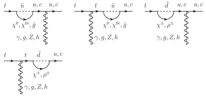
Figure 1: Self-energy diagrams contributing to $t\rightarrow qV,qh$ in the MRSSM, where $\gamma$, $g$ and $Z$ are denoted by the wavy lines, and $h$ is denoted by the dashed lines.

Figure 2: Triangle diagrams contributing to $t\rightarrow qV,qh$ in the MRSSM, where $\gamma$, $g$ and $Z$ are denoted by the wavy lines, and $h$ is denoted by the dashed lines.

The relevant Feynman diagrams contributing to $t\rightarrow qV,qh$ in the MRSSM are presented in Fig.1 and Fig.2, where $\chi^{0}$/$\chi^{0c}$ denote the neutralinos/anti-neutralinos, and $\tilde{g}$ denote the gluinos and anti-gluinos. All the self-energy diagrams contribute to the $t\rightarrow qV,qh$ decays. Not all of the triangle diagrams contribute to the $t\rightarrow qV,qh$ decays owing to the fact that the coupling between the boson $V/h$ and the loop particles may not exist. From Fig.2 we see that the diagram containing two $\tilde{g}$ is absent for $t\rightarrow qZ,qh$, the diagrams containing two $\chi^{0}$/$\chi^{0c}$ or two $\tilde{g}$ are absent for $t\rightarrow q\gamma$, and the diagrams containing two $\chi^{\pm}$, two $\rho^{\pm}$ or two $\chi^{0}$/$\chi^{0c}$ are absent for $t\rightarrow qg$. The general form of the amplitude in Fig.1 and Fig.2 is given by Lopez1997 ; Chiang ; Bolanos

$${\cal M}(t\rightarrow q\gamma) = \bar{u}_{q}[\gamma^{\mu}(F^{L}_{1\gamma}P_{L}+F^{R}_{1\gamma}P_{R})+i\sigma^{\mu\nu}q_{\nu}(F^{L}_{2\gamma}P_{L}+F^{R}_{2\gamma}P_{R})]u_{t}\epsilon_{\mu},$$

$${\cal M}(t\rightarrow qg) = \bar{u}_{q}[T^{a}\gamma^{\mu}(F^{L}_{1g}P_{L}+F^{R}_{1g}P_{R})+iT^{a}\sigma^{\mu\nu}q_{\nu}(F^{L}_{2g}P_{L}+F^{R}_{2g}P_{R})]u_{t}\epsilon_{\mu},$$

$${\cal M}(t\rightarrow qZ) = \bar{u}_{q}[\gamma^{\mu}(F^{L}_{1Z}P_{L}+F^{R}_{1Z}P_{R})+\frac{i\sigma^{\mu\nu}q_{\nu}}{m_{t}+m_{q}}(F^{L}_{2Z}P_{L}+F^{R}_{2Z}P_{R})]u_{t}\epsilon_{\mu},$$

$${\cal M}(t\rightarrow qh) = \bar{u}_{q}(F^{L}_{h}P_{L}+F^{R}_{h}P_{R})u_{t}h,$$ (25)

where $q_{\nu}$ is the momentum of outgoing gauge boson, and $\epsilon_{\mu}$ is the polarization vector of the outgoing gauge boson. $P_{L/R}$ = $\frac{1}{2}(1\mp\gamma_{5})$ and $\sigma^{\mu\nu}$ = $\frac{i}{2}[\gamma^{\mu},\gamma^{\nu}]$. $T^{a}$ are the generators of $SU(3)_{C}$. The contribution from the tensor operators in Eq.(25) for $t\rightarrow q\gamma,qg$ can be neglected in the MRSSM since the coefficients $F^{L/R}_{2\gamma}$ and $F^{L/R}_{2g}$ that calculated from the Feynman diagrams in Fig.1 and Fig.2 are zero. Then, the branching ratios for $t\rightarrow qV,qh$ are given by Lopez1997 ; Chiang ; Bolanos

$$BR(t\rightarrow q\gamma) = \frac{m_{t}}{32\pi\Gamma_{t}}[2(F^{L}_{1\gamma})^{2}+2(F^{R}_{1\gamma})^{2}-6m_{t}(F^{L}_{1\gamma}F^{R}_{2\gamma}+F^{R}_{1\gamma}F^{L}_{2\gamma})$$

$$+2m^{2}_{t}(F^{L}_{2\gamma})^{2}+2m^{2}_{t}(F^{R}_{2\gamma})^{2}],$$

$$BR(t\rightarrow qg) = \frac{m_{t}}{24\pi\Gamma_{t}}[2(F^{L}_{1g})^{2}+2(F^{R}_{1g})^{2}-6m_{t}(F^{L}_{1g}F^{R}_{2g}+F^{R}_{1g}F^{L}_{2g})$$

$$+2m^{2}_{t}(F^{L}_{2g})^{2}+2m^{2}_{t}(F^{R}_{2g})^{2}],$$

$$BR(t\rightarrow qZ) = \frac{(m_{t}^{2}-m^{2}_{Z})^{2}}{32\pi m^{3}_{t}\Gamma_{t}}[(2+\frac{m^{2}_{t}}{m^{2}_{Z}})(|F^{L}_{1Z}|^{2}+|F^{R}_{1Z}|^{2})+(2+\frac{m^{2}_{Z}}{m^{2}_{t}})$$

$$\times(|F^{L}_{2Z}|^{2}+|F^{R}_{2Z}|^{2})-6Re(F^{L}_{1Z}F^{R*}_{2Z}+F^{R}_{1Z}F^{L*}_{2Z})]$$

$$BR(t\rightarrow qh) = \frac{\lambda^{1/2}(m_{t}^{2},m_{h}^{2},m_{q}^{2})}{8\pi m^{3}_{t}\Gamma_{t}}[\frac{m_{t}^{2}+m_{q}^{2}-m_{h}^{2}}{2}(|F^{L}_{h}|^{2}+|F^{R}_{h}|^{2})$$ (26)

$$+2m_{t}m_{q}Re(F^{L}_{h}F^{R*}_{h})],$$

where $\Gamma_{t}$ denotes the total width of the top quark and $\lambda(x,y,z)$=$x^{2}+y^{2}+z^{2}-2(xy+xz+yz)$.

The calculation of the branching ratios is carried out by using the spectrum generator SPheno-4.0.5 SPheno1 ; SPheno2 , where the model implementations are generated by the public code SARAH-4.15.1 SARAH ; SARAH1 ; SARAH2 ; Flavor ; Flavor2 . The generic expressions for the Wilson coefficients in Eq.(25) are derived with the help of the Mathematica package PreSARAH-1.0.3 which uses FeynArts and FormCalc Hahn1999 ; Hahn2000 ; Hahn2001 ; Hahn2004 ; Hahn2005 ; Hahn2014 to compute the generic expressions for the required Wilson coefficients at the tree- and 1-loop levels. The conventions in Eq.(25) are different from those presented in Ref.Flavor . The Wilson coefficients in Eq.(25) and Ref.Flavor are related by $F^{L/R}_{2\gamma}=Q^{L/R}_{1}$, $F^{L/R}_{2g}=Q^{L/R}_{2}$. By adding the new operators, the generic expressions for $F^{L/R}_{1\gamma}$, $F^{L/R}_{1Z}$, $F^{L/R}_{2Z}$, $F^{L/R}_{1g}$ and $F^{L/R}_{h}$ in Eq.(25) are derived with PreSARAH. Details on how to implement the new operators and obtain the analytical expressions for their Wilson coefficients can be found in Ref.Flavor . The explicit expressions for the Wilson coefficients in the MRSSM are obtained by adapting the generic expressions to the specific details of the MRSSM by SARAH. The Fortran code is written by authors to relate the Wilson coefficients in Eq.(25) and the decay widths in Eq.(26), and this code is used by SARAH to generate the Fortran modules for SPheno. The numerical calculation of BR($t\rightarrow qV,qh$) is done by SPheno. Details on how to implement new observables $t\rightarrow qV,qh$ in SPheno can be found in Ref.Flavor2 .

In the following we present the detailed expressions for the Wilson coefficients. The coefficients are left-right symmetric, i.e., $F^{R}_{1V}$=$F^{L}_{1V}$($L\leftrightarrow R$), $F^{R}_{2V}$=$F^{L}_{2V}$($L\leftrightarrow R$), $F^{R}_{h}$=$F^{L}_{h}$($L\leftrightarrow R$). All coefficients that are not explicitly listed are zero and all charge factors that are not explicitly listed are 1.

The coefficients correspond to the 1st and 3rd diagram in Fig.1 are

$$F^{L,FS}_{1V} = \frac{Q_{FS}C^{qqV}_{R}}{m_{t}^{2}-m_{q}^{2}}(C^{tFS*}_{R}C^{qFS}_{R}m_{t}m_{F}B_{0}(m_{t}^{2},m_{F}^{2},m_{S}^{2})-C^{tFS*}_{L}C^{qFS}_{R}m_{t}^{2}B_{1}(m_{t}^{2},m_{F}^{2},m_{S}^{2})$$

$$-C^{tFS*}_{R}C^{qFS}_{L}m_{t}m_{q}B_{1}(m_{t}^{2},m_{F}^{2},m_{S}^{2})+C^{tFS*}_{L}C^{qFS}_{L}m_{F}m_{q}B_{0}(m_{t}^{2},m_{F}^{2},m_{S}^{2})),$$

and the coefficients correspond to the 2nd and 4th diagram in Fig.1 are

$$F^{L,FS}_{1V} = \frac{Q_{FS}C^{ttV}_{R}}{m_{q}^{2}-m_{t}^{2}}(C^{qFS}_{L}C^{tFS*}_{L}m_{q}m_{F}B_{0}(m_{q}^{2},m_{F}^{2},m_{S}^{2})-C^{qFS}_{R}C^{tFS*}_{L}m_{q}^{2}B_{1}(m_{q}^{2},m_{F}^{2},m_{S}^{2})$$

$$-C^{qFS}_{L}C^{tFS*}_{R}m_{q}m_{t}B_{1}(m_{q}^{2},m_{F}^{2},m_{S}^{2})+C^{qFS}_{R}C^{tFS*}_{R}m_{F}m_{t}B_{0}(m_{q}^{2},m_{F}^{2},m_{S}^{2})),$$

where $FS\in\{\chi^{\pm}\tilde{d},\rho^{\pm}\tilde{d},\chi^{0}\tilde{u},\chi^{0c}\tilde{u},\tilde{g}\tilde{u}\}$. The charge factor $Q_{FS}=4/3$ for $FS\in\{\tilde{g}\tilde{u}\}$ and $F^{L,FS}_{h}=F^{R,FS}_{1V}(V\rightarrow h)$.

The coefficients correspond to the 2nd and 3rd diagram in Fig.2 are

$$F^{L,FS_{1}S_{2}}_{1V} = -2Q_{FS_{1}S_{2}}C^{tFS_{1}*}_{L}C^{qFS_{2}}_{R}C^{S_{1}S_{2}V}C_{00}(m_{F}^{2},m_{S_{2}}^{2},m_{S_{1}}^{2}),$$

$$F^{L,FS_{1}S_{2}}_{2Z} = 2Q_{FS_{1}S_{2}}C^{qFS_{2}}_{L}C^{S_{1}S_{2}Z}(C^{tFS_{1}*}_{R}m_{t}C^{\prime}_{0}(m_{F}^{2},m_{S_{2}}^{2},m_{S_{1}}^{2})$$

$$-C^{tFS_{1}*}_{L}m_{F}C^{\prime}_{2}(m_{F}^{2},m_{S_{2}}^{2},m_{S_{1}}^{2})),$$

$$F^{L,FS_{1}S_{2}}_{h} = -Q_{FS_{1}S_{2}}C^{tFS_{1}*}_{L}C^{qFS_{2}}_{L}C^{S_{1}S_{2}h}m_{F_{1}}C_{0}(m_{F}^{2},m_{S_{2}}^{2},m_{S_{1}}^{2}),$$

where $FS_{1}S_{2}\in\{\chi^{\pm}\tilde{d}\tilde{d},\rho^{\pm}\tilde{d}\tilde{d},\chi^{0}\tilde{u}\tilde{u},\chi^{0c}\tilde{u}\tilde{u},\tilde{g}\tilde{u}\tilde{u}\}$. For $FS_{1}S_{2}$=$\tilde{g}\tilde{u}\tilde{u}$, the charge factor $Q_{FS_{1}S_{2}}$ is $-1/6$ for $t\rightarrow qg$ and $4/3$ for $t\rightarrow q\gamma,qZ,qh$. The coefficients correspond to the 1st, 4th and 5th diagram in Fig.2 are

$$F^{L,F_{1}F_{2}S}_{1V} = -Q_{F_{1}F_{2}S}C^{qF_{2}S}_{R}(2C^{tF_{1}S*}_{R}m_{t}(C^{F_{1}F_{2}V}_{R}m_{F_{1}}C_{1}(m^{2}_{F_{2}},m^{2}_{F1},m^{2}_{S})-C^{F_{1}F_{2}V}_{L}m_{F_{2}}$$

$$\times(C_{0}(m^{2}_{F_{2}},m^{2}_{F_{1}},m^{2}_{S})+C_{1}(m^{2}_{F_{2}},m^{2}_{F_{1}},m^{2}_{S})))+C^{tF_{1}S*}_{L}(-2C^{F_{1}F_{2}V}_{L}m_{F_{1}}m_{F_{2}}$$

$$\times C_{0}(m^{2}_{F_{2}},m^{2}_{F_{1}},m^{2}_{S})+C^{F_{1}F_{2}V}_{R}(B_{0}(0,m^{2}_{F_{1}},m^{2}_{F_{2}})-2C_{00}(m^{2}_{F_{2}},m^{2}_{F_{1}},m^{2}_{S})$$

$$+m^{2}_{t}C_{1}(m^{2}_{F_{2}},m^{2}_{F_{1}},m^{2}_{S})+m^{2}_{S}C_{0}(m^{2}_{F_{2}},m^{2}_{F_{1}},m^{2}_{S})))),$$

$$F^{L,F_{1}F_{2}S}_{2Z} = 2Q_{F_{1}F_{2}S}C^{qF_{2}S}_{L}(C^{tF_{1}S*}_{R}C^{F_{1}F_{2}Z}_{L}m_{t}C_{12}(m^{2}_{F_{2}},m^{2}_{F_{1}},m^{2}_{S})-C^{tF_{1}S*}_{L}C^{F_{1}F_{2}Z}_{L}m_{F_{1}}$$

$$\times C_{1}(m^{2}_{F_{2}},m^{2}_{F_{1}},m^{2}_{S})+C^{tF_{1}S*}_{L}C^{F_{1}F_{2}Z}_{R}m_{F_{2}}C^{\prime}_{0}(m^{2}_{F_{2}},m^{2}_{F_{1}},m^{2}_{S})),$$

$$F^{L,F_{1}F_{2}S}_{h} = -Q_{F_{1}F_{2}S}C^{tF_{1}S*}_{L}C^{qF_{2}S}_{L}(2C^{F_{1}F_{2}h}_{L}m_{F_{1}}m_{F_{2}}C_{0}(m^{2}_{F_{2}},m^{2}_{F_{1}},m^{2}_{S})+C^{F_{1}F_{2}h}_{R}(m^{2}_{S}$$

$$\times C_{0}(m^{2}_{F_{2}},m^{2}_{F_{1}},m^{2}_{S})+B_{0}(0,m^{2}_{F_{1}},m^{2}_{F_{2}}))),$$

where $F_{1}F_{2}S\in\{\chi^{\pm}\chi^{\pm}\tilde{d},\rho^{\pm}\rho^{\pm}\tilde{d},\chi^{0}\chi^{0}\tilde{u},\chi^{0c}\chi^{0c}\tilde{u},\tilde{g}\tilde{g}\tilde{u}\}$. The loop integrals $B_{\{0,1\}}$ and $C_{\{0,1,2,00,12,22\}}$ are the Passarino-Veltman functions in the limit of vanishing external momenta. The loop integrals $C^{\prime}_{\{0,2\}}$ are the combinations of $C_{\{0,1,2\}}$ and $C_{\{2,12,22\}}$, respectively. The explicit expressions of the integrals can be found in references SPheno1 ; SPheno2 ; Flavor ; Flavor2 .

III Numerical Analysis

The numerical computation of the one loop corrections to $t\rightarrow qV,qh$ in the MRSSM is done by using the full evaluation within the framework of SPheno. The computation is done in a low scale version of SPheno and all free parameters are given at the SUSY scale. In the numerical analysis, we will use one set of benchmark points which are taken from Ref.Diessner2014 and Ref.Diessner2019 , and display them in Eq.(27). All mass parameters in Eq.(27) are given in GeV or GeV². In the following numerical analysis, the values in Eq.(27) will be used as default. Note that, the off-diagonal entries of the squark mass matrices $m^{2}_{\tilde{q}}$, $m^{2}_{\tilde{u}}$, $m^{2}_{\tilde{d}}$ and slepton mass matrices $m^{2}_{l}$, $m^{2}_{r}$ in Eq.(27) are zero, i.e., the flavor mixing of squark and slepton is absent.

$$\begin{array}[]{l}\tan\beta=3,B_{\mu}=500^{2},\lambda_{d}=1.0,\lambda_{u}=-0.8,\Lambda_{d}=-1.2,\Lambda_{u}=-1.1,\\ M_{D}^{B}=550,M_{D}^{W}=600,M_{D}^{O}=1500,\mu_{d}=\mu_{u}=500,v_{S}=5.9,v_{T}=-0.38,\\ (m^{2}_{l})_{11}=(m^{2}_{l})_{22}=(m^{2}_{l})_{33}=(m^{2}_{r})_{11}=(m^{2}_{r})_{22}=(m^{2}_{r})_{33}=1000^{2},\\ (m^{2}_{\tilde{q}})_{11}=(m^{2}_{\tilde{u}})_{11}=(m^{2}_{\tilde{d}})_{11}=(m^{2}_{\tilde{q}})_{22}=(m^{2}_{\tilde{u}})_{22}=(m^{2}_{\tilde{d}})_{22}=2500^{2},\\ (m^{2}_{\tilde{q}})_{33}=(m^{2}_{\tilde{u}})_{33}=(m^{2}_{\tilde{d}})_{33}=1000^{2},m_{T}=3000,m_{S}=2000.\end{array}$$ (27)

These benchmark points make it possible to accommodate proper Higgs boson mass of around 125 GeV in the MRSSM where the lightest Higgs boson is SM-like. Using HiggsBounds and HiggsSignals, the Higgs sector of the benchmark points is checked against existing experimental data. Using Vevacious, the Higgs potential of the MRSSM is checked for possible presence of deeper minima in the parameter space. The W boson mass is found in agreement with the experimental value from combined LEP and Tevatron and low energy B meson physics observables are found agreement with measurements. It is known to all that the experimental observables of $\bar{B}\rightarrow X_{s}\gamma$ and $B^{0}_{d,s}\rightarrow\mu^{+}\mu^{-}$ can be adopted to constraint the relevant parameter space. The present experimental data for BR($\bar{B}\rightarrow X_{s}\gamma$), BR($B^{0}_{s}\rightarrow\mu^{+}\mu^{-}$) and BR($B^{0}_{d}\rightarrow\mu^{+}\mu^{-}$) are BR($\bar{B}\rightarrow X_{s}\gamma$) = $(3.32\pm 0.15)\times 10^{-4}$, BR($B^{0}_{s}\rightarrow\mu^{+}\mu^{-}$) = $(3.0\pm 0.4)\times 10^{-9}$ and BR($B^{0}_{d}\rightarrow\mu^{+}\mu^{-}$) = $(1.1^{+1.4}_{-1.3})\times 10^{-10}$. At the benchmark points, the predicted BR($\bar{B}\rightarrow X_{s}\gamma$), BR($B^{0}_{s}\rightarrow\mu^{+}\mu^{-}$) and BR($B^{0}_{d}\rightarrow\mu^{+}\mu^{-}$) in the MRSSM are BR($\bar{B}\rightarrow X_{s}\gamma$) = $3.47\times 10^{-4}$, BR($B^{0}_{s}\rightarrow\mu^{+}\mu^{-}$) = $3.16\times 10^{-9}$, BR($B^{0}_{d}\rightarrow\mu^{+}\mu^{-}$) = $1.02\times 10^{-10}$.

The predicted W boson mass in the MRSSM is comparable with the result from the combination of the Large Electron-Positron collider and the Fermilab Tevatron collider measurements CDF2013 , the result from the ATLAS collaboration ATLAS2018 and the result from the LHCb Collaboration LHCb2022 which is more precise than the LEP result. By changing the values of some parameters, e.g. $m_{SUSY}$, $v_{T}$, $\Lambda_{u}$ and $\Lambda_{d}$, the recent result on W boson mass from CDF collaboration CDF2022 can also be accommodated in the MRSSM Diessner2019 ; Athron2022 . It is noted that these parameters have very small effect on the prediction of BR($t\rightarrow qV,qh$) which take values along a narrow band.

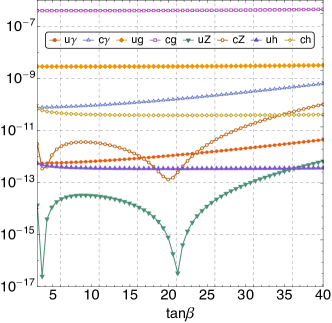
Figure 3: Dependence of BR($t\rightarrow qV,qh$) on the ratio tan$\beta$ in the MRSSM.

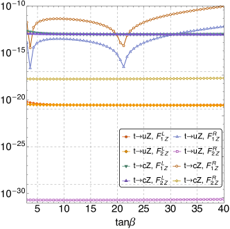
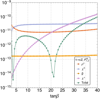
Figure 4: Dependence of BR($t\rightarrow qZ,F^{L/R}_{1Z/2Z}$) and BR($t\rightarrow cZ,F^{R}_{1Z}$) on the ratio tan$\beta$ in the MRSSM.

Taking values in Eq.(27), we plot the predictions of BR($t\rightarrow qV,qh$) versus the ratio tan$\beta$ in Fig.3. The varying ratio tan$\beta$ has very little effect on the predicted BR($t\rightarrow qg,qh$). The predicted BR($t\rightarrow q\gamma$) would increase slowly with the increase of tan$\beta$ by about one order of magnitude. There are two deep decreases at tan$\beta\approx 4$ and tan$\beta\approx 21$ for BR($t\rightarrow qZ$). In the left panel of Fig.4 we plot the predictions of BR($t\rightarrow qZ,F^{L/R}_{1Z/2Z}$) versus tan$\beta$ by considering the contributions from the Wilson coefficients $F^{L/R}_{1Z/2Z}$ separately. The varying ratio tan$\beta$ has very little effect on the predicted BR($t\rightarrow qZ$) when only one of the coefficients $F^{L}_{1Z}$, $F^{L}_{2Z}$ and $F^{R}_{2Z}$ is considered. There are two deep decreases at tan$\beta\approx 4$ and tan$\beta\approx 21$ for BR($t\rightarrow qZ$) with $F^{R}_{1Z}$, and this can explain where the two decreases in Fig.3 come from. In the right panel of Fig.4 we plot the predictions of BR($t\rightarrow cZ,F^{R}_{1Z}$) versus tan$\beta$ by considering the contributions from $\rho^{\pm}$, $\chi^{0}(\chi^{0c})$, $\tilde{g}$ and $\chi^{\pm}$ separately, where the coefficients $F^{L}_{1Z}$, $F^{L}_{2Z}$ and $F^{R}_{2Z}$ are set zero and the ‘Total’ line in the right panel is same with the ‘$t\rightarrow cZ,F^{R}_{1Z}$’ line in the left panel.

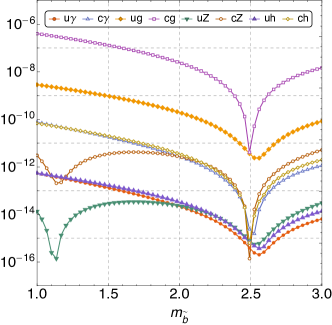
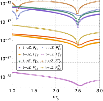
Figure 5: Dependence of BR($t\rightarrow qV,qh$) and BR($t\rightarrow qZ,F^{L/R}_{1Z/2Z}$) on the third generation squark mass $m_{\tilde{b}}$ in the MRSSM. $m_{\tilde{b}}$ is given in TeV.

Taking values in Eq.(27), we plot the predictions of BR($t\rightarrow qV,qh$) versus the third generation squark mass $m_{\tilde{b}}$ in the left panel of Fig.5, where $(m^{2}_{\tilde{q}})_{33}$ = $(m^{2}_{\tilde{u}})_{33}$ = $(m^{2}_{\tilde{d}})_{33}$ =$m^{2}_{\tilde{b}}$. The mass parameter $m_{\tilde{b}}$ is given in TeV. At $m_{\tilde{b}}$ = 1 TeV, the following hierarchies are shown, BR($t\rightarrow cg$) $>$ BR($t\rightarrow ug$) $>$ BR($t\rightarrow c\gamma$) $>$ BR($t\rightarrow cZ$) $>$ BR($t\rightarrow u\gamma$) $>$ BR($t\rightarrow uZ$) and BR($t\rightarrow ch$) $>$ BR($t\rightarrow uh$). The same hierarchies appear in the SM as shown in Table.1 and in several new physics Yang2009 ; Gao ; Chiang ; Yang2018 . In some models, the two hierarchies may be violated (e.g.Lopez1997 ; Yang1998 ; Lu2003 ; Liu2004 ; Frank2005 ; Hou2007 ; Cao2007 ) and the branching ratios BR($t\rightarrow cV,ch$) could be roughly the same order of magnitude (e.g.Li1994 ; Bolanos ). As shown in the left panel of Fig.5, there is a narrow cancellation region around $m_{\tilde{b}}$ = 2.5 TeV for BR($t\rightarrow qV,qh$). Here the predicted BR($t\rightarrow qV,qh$) are very close to the SM predictions, making it effectively unobservable at the future experiments. This cancellation originates from the degeneration of the squark mass in matrices $m^{2}_{\tilde{q}}$, $m^{2}_{\tilde{d}}$ and $m^{2}_{\tilde{u}}$. There is another narrow cancellation region around $m_{\tilde{b}}$ = 1 TeV for BR($t\rightarrow qZ$) and, to explain this, we show the the predicted BR($t\rightarrow qZ,F^{L/R}_{1Z/2Z}$) versus the third generation squark mass $m_{\tilde{b}}$ in the right panel of Fig.5 where only the contribution form the indicated coefficient $F^{L/R}_{1Z/2Z}$ is considered. There is a deep decrease at $m_{\tilde{b}}\approx 1.1$ GeV for BR($t\rightarrow qZ,F^{R}_{1Z}$), and this can explain where the left decrease in the left panel of Fig.5 comes from.

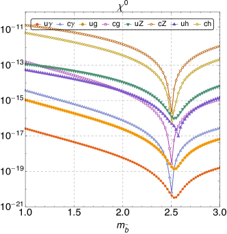
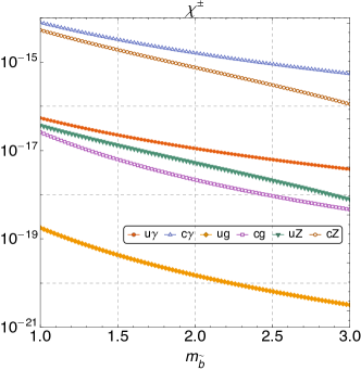
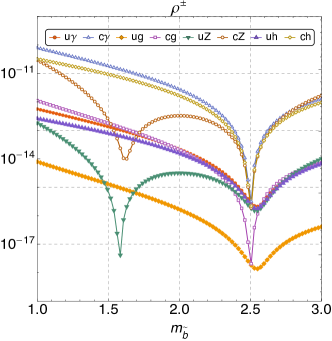
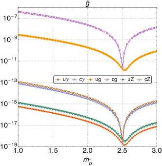
Figure 6: Dependence of BR($t\rightarrow qV,qh$) with contributions from $\chi^{0}$, $\chi$-chargino, $\rho$-chargino and $\tilde{g}$ on the third generation squark mass $m_{\tilde{b}}$ in the MRSSM. The values of BR($t\rightarrow qV,qh$) are given by only the listed contribution with all others set to zero. $m_{\tilde{b}}$ is given in TeV. Contributions from $\chi^{\pm}$ and $\tilde{g}$ are very small ($\leq 10^{-25}$) for BR($t\rightarrow qh$) and not shown in the figure.

In Fig.6, we independently plot the contributions to BR($t\rightarrow qV,qh$) from the neutralino $\chi^{0}$, $\chi$-chargino, $\rho$-chargino and gluino $\tilde{g}$ versus the third generation squark mass $m_{\tilde{b}}$. For BR($t\rightarrow q\gamma$), we observe that $\rho$-chargino contribution dominates the predictions, $\chi^{0}$, $\tilde{g}$ and $\chi$-chargino contributions are less dominant or negligible. For BR($t\rightarrow qg$),$\tilde{g}$ contribution is dominant, $\rho$-chargino and $\chi^{0}$ contributions are less dominant and $\chi$-chargino contribution is negligible. For BR($t\rightarrow qZ$), contributions from $\chi^{0}$ and $\rho$-chargino are comparable and both dominate the predictions on BR($t\rightarrow qZ$), $\tilde{g}$ and $\chi^{\pm}$ contribution are less dominant or negligible. As mentioned above, there is a narrow cancellation region around $m_{\tilde{b}}$ = 1 TeV for BR($t\rightarrow qZ$) in the Fig.5 and this can be explained by the interference between the corrections from $\rho$-chargino sector and that from $\chi^{0}$ sector. For BR($t\rightarrow qh$), contributions from $\chi^{0}$ and $\rho$-chargino are comparable and both dominate the predictions on BR($t\rightarrow qh$). Contributions from $\chi^{\pm}$ and $\tilde{g}$ are very small for BR$(t\rightarrow qh)$ ($\leq 10^{-25}$) and negligible. This is due to the fact that the $\chi^{\pm}$ (or $\tilde{g}$)-quark-squark coupling is eithor left-handed or right-handed. To understand this point, we take the last diagram in Fig.1 for example. For the $\rho^{\pm}$-mediated diagrams, the factors $F^{L/R}_{h}$ (e.g. $t\rightarrow uh$) in Eq.(25) are proportional to the mass of particles and read as follows

$$F^{L}_{h} \propto C^{u\rho^{\pm}\tilde{d}}_{R}C^{\ast t\rho^{\pm}\tilde{d}}_{R}B_{0}m_{u}m_{\rho^{\pm}}-C^{u\rho^{\pm}\tilde{d}}_{L}C^{\ast t\rho^{\pm}\tilde{d}}_{R}B_{1}m^{2}_{u}-C^{u\rho^{\pm}\tilde{d}}_{R}C^{\ast t\rho^{\pm}\tilde{d}}_{L}B_{1}m_{u}m_{t}$$

$$+C^{u\rho^{\pm}\tilde{d}}_{L}C^{\ast t\rho^{\pm}\tilde{d}}_{L}B_{0}m_{t}m_{\rho^{\pm}},$$

$$F^{R}_{h} \propto F^{L}_{h}(L\leftrightarrow R)$$ (28)

where $C^{u\rho^{\pm}\tilde{d}}_{L/R}$ ($C^{\ast t\rho^{\pm}\tilde{d}}_{L/R}$) stand for the left-handed or right-handed couplings of the interaction between $\rho$-chargino and up-type quark/squark. $B_{0}$ and $B_{1}$ are the two-point loop integrals. For the $\chi^{\pm}$-mediated diagrams, due to the fact that the coupling $C^{u\chi^{\pm}\tilde{d}}$ is left-handed, only the term which is proportional to $B_{1}m^{2}_{u}$ in Eq.(28) is nonzero ($B_{1}m_{u}m_{t}$ for $F^{R}_{h}$). Thus $\frac{BR(t\rightarrow qh,\;\chi^{\pm}\;mediated)}{BR(t\rightarrow qh,\;\rho^{\pm}\;mediated)}\propto\frac{m^{2}_{q}}{m^{2}_{\rho^{\pm}}}$ and, comparing with $\rho$-chargino, the contribution from $\chi$-chargino is neglible. A similar discussion can be given between the $\chi^{0}$-mediated diagrams and the $\tilde{g}$-mediated diagrams.

As discussed in several articles Bejar2001 ; Guasch1999 ; Cao2007 ; Liu2004 ; Delepine2004 ; Dedes2014 ; Frank2005 , the off-diagonal entries of the soft breaking terms $m_{\tilde{q}}^{2}$, $m_{\tilde{u}}^{2}$ and $m_{\tilde{d}}^{2}$ can strongly affect the predicted BR($t\rightarrow qV,qh$). In the following we will investigate the influence of these squark flavor mixing parameters on BR($t\rightarrow qV,qh$) in the MRSSM. Using the mass insertion method, the off-diagonal entries of the squark mass matrices $m_{\tilde{q}}^{2}$, $m_{\tilde{u}}^{2}$ and $m_{\tilde{d}}^{2}$ are parameterized by $(m^{2}_{X})_{IJ}=\delta^{IJ}_{X}\sqrt{(m^{2}_{X})_{II}(m^{2}_{X})_{JJ}}$ where $X=\tilde{q},\tilde{u},\tilde{d}$ and $I,J=1,2,3$. Note that, the default value of the off-diagonal entries of the squark mass matrices $m^{2}_{\tilde{q}}$, $m^{2}_{\tilde{u}}$, $m^{2}_{\tilde{d}}$ in Eq.(27) are zero.

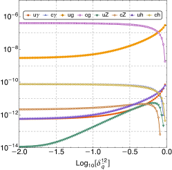
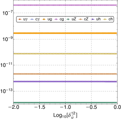
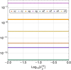
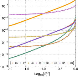
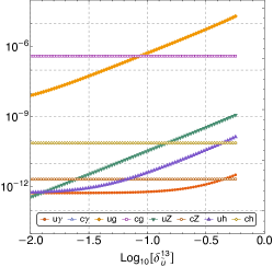
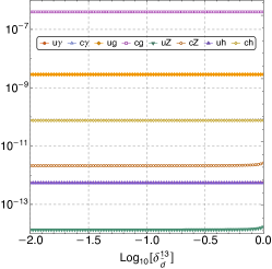
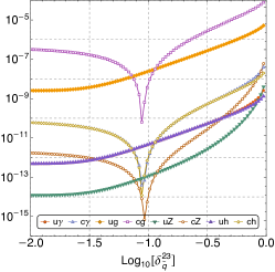
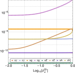
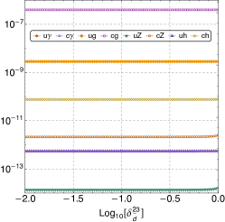
Figure 7: Dependence of BR($t\rightarrow qV,qh$) on the base-10 logarithm of the squark flavor mixing parameters $\delta^{IJ}_{\tilde{q}}$,$\delta^{IJ}_{\tilde{u}}$ and $\delta^{IJ}_{\tilde{d}}$ .

In Fig.7 the predictions for BR($t\rightarrow qV,qh$) are shown as a function of the mass insertion parameters $\delta^{IJ}_{\tilde{q}(\tilde{u},\tilde{d})}$. In all plots only the indicated $\delta^{IJ}_{\tilde{q}(\tilde{u},\tilde{d})}$ is varied with all other mass insertions set to zero. The experimental data for BR($\bar{B}\rightarrow X_{s}\gamma$), BR($B^{0}_{s}\rightarrow\mu^{+}\mu^{-}$) and BR($B^{0}_{d}\rightarrow\mu^{+}\mu^{-}$) are used to constrain these mass insertion parameters. The results show that varying the parameters $\delta^{12}_{\tilde{u}}$,$\delta^{23}_{\tilde{u}}$,$\delta^{12}_{\tilde{d}}$,$\delta^{13}_{\tilde{d}}$ and $\delta^{23}_{\tilde{d}}$ has very small effect on the predictions of BR($t\rightarrow uV,uh$) and varying the parameters $\delta^{12}_{\tilde{u}}$,$\delta^{13}_{\tilde{u}}$,$\delta^{12}_{\tilde{d}}$,$\delta^{13}_{\tilde{d}}$ and $\delta^{23}_{\tilde{d}}$ has very small effect on the predictions of BR($t\rightarrow cV,ch$), both of which take values along a narrow band. The predictions of BR($t\rightarrow uV,uh$) increase with the increase of $\delta^{12}_{\tilde{q}}$,$\delta^{13}_{\tilde{q}}$,$\delta^{23}_{\tilde{q}}$ and $\delta^{13}_{\tilde{u}}$, and the predictions of BR($t\rightarrow ug$) could be enhanced to be close to the present experimental bound while others are still several orders of magnitude below the present experimental bounds. The predictions of BR($t\rightarrow cV,ch$) increase with the increase of $\delta^{13}_{\tilde{q}}$ and $\delta^{23}_{\tilde{u}}$ but the decrease of $\delta^{12}_{\tilde{q}}$. There is a deep decrease at $Log_{10}[\delta^{23}_{\tilde{q}}]\sim-1.0$ for BR($t\rightarrow cV,ch$) and this is due to the destructive interference. This behavior in the MRSSM is similar to that in the MSSM Cao2007 and the left-right supersymmetric model Frank2005 .

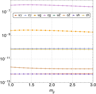
Figure 8: Dependence of BR($t\rightarrow qV,qh$) on the gluino mass $m_{\tilde{g}}$. $m_{\tilde{g}}$ is given in TeV.

Taking values in Eq.(27), we plot the predictions of BR($t\rightarrow qV,qh$) versus the gluino mass $m_{\tilde{g}}$ in Fig.8. The results show that varying gluino mass $m_{\tilde{g}}$ has very small effect on the predictions of BR($t\rightarrow qV,qh$) which take values along a narrow band. This may be different from that in the MSSM where the predictions of BR($t\rightarrow qV,qh$) decrease quickly as the gluino mass increases Li1994 ; Guasch1999 ; Cao2007 .

IV Conclusions

In this work, taking account of the constraints from the experimental data on the parameter space, we analyze the FCNC processes $t\rightarrow qV,qh$ in the framework of the minimal R-symmetric supersymmetric standard model. In the MRSSM, Majorana gaugino masses, $\mu$ term, $A$ terms and all the left-right squark and slepton mass mixings are absent according to the R-symmetry and this makes the predictions for BR($t\rightarrow qV,qh$) be different from those in the MSSM. We show the dependence of BR($t\rightarrow qV,qh$) on the ratio tan$\beta$, the third generation squark mass $m_{\tilde{b}}$, the squark flavor mixing parameters $\delta^{IJ}_{\tilde{q},\tilde{u},\tilde{d}}$ and the gluino mass $m_{\tilde{g}}$ and independently consider the contributions to the branching ratio BR($t\rightarrow qV,qh$) from various supersymmetry particles.

At the benchmark points, the predicted BR($t\rightarrow u\gamma,c\gamma$) are at the level of $\mathcal{O}(10^{-13})$ and $\mathcal{O}(10^{-11})$, respectively, and both are three orders of magnitude above the SM prediction. Considering the effect from $\delta^{13}_{\tilde{q}}$, the predicted BR($t\rightarrow u\gamma,c\gamma$) can be enhanced to be $\mathcal{O}(10^{-9}\sim 10^{-10})$, which are four and five orders of magnitude below the estimated branching ratios at the HL-LHC and FCC-hh Aguilar2017 , respectively. The predicted BR($t\rightarrow uZ,cZ$) are at the level of $\mathcal{O}(10^{-14})$ and $\mathcal{O}(10^{-12})$, and they are three and two orders of magnitude above the SM prediction, respectively. Considering the effect from $\delta^{13}_{\tilde{q}}$ and $\delta^{23}_{\tilde{u}}$, the predicted BR($t\rightarrow uZ,cZ$) can be enhanced to be $\mathcal{O}(10^{-10}\sim 10^{-11})$, which are four and five orders of magnitude below the estimated branching ratios at the HL-LHC and FCC-hh Aguilar2017 , respectively. The predicted BR($t\rightarrow uh,ch$) are at the level of $\mathcal{O}(10^{-13})$ and $\mathcal{O}(10^{-11})$, respectively, and both are four orders of magnitude above the SM prediction. Considering the effect from $\delta^{13}_{\tilde{q}}$ and $\delta^{23}_{\tilde{u}}$, the predicted BR($t\rightarrow uh,ch$) can be enhanced to be $\mathcal{O}(10^{-9})$, and both are four orders of magnitude below the estimated branching ratios at the HE-LHC and FCC-hh YJZhang . The predicted BR($t\rightarrow ug,cg$) are at the level of $\mathcal{O}(10^{-7})$ and $\mathcal{O}(10^{-9})$, and they are two and four orders of magnitude below the present experimental bound, respectively. By changing the parameters $\delta^{13}_{\tilde{q}}$, $\delta^{23}_{\tilde{q}}$, $\delta^{13}_{\tilde{u}}$ and $\delta^{23}_{\tilde{u}}$, the predicted BR($t\rightarrow ug,cg$) can be enhanced to be $\mathcal{O}(10^{-5}-10^{-6})$ and this can be tested at the HL-LHC and FCC-hh CMSqg ; Oyulmaz . Thus, the processes $t\rightarrow ug,cg$ are very promising to be observed in the near future experiment.