ACTIVE: A Deep Model for Sperm and Impurity Detection in Microscopic Videos

Abstract

The accurate detection of sperms and impurities is a very challenging task, facing problems such as the small size of targets, indefinite target morphologies, low contrast and resolution of the video, and similarity of sperms and impurities. So far, the detection of sperms and impurities still largely relies on the traditional image processing and detection techniques which only yield limited performance and often require manual intervention in the detection process, therefore unfavorably escalating the time cost and injecting the subjective bias into the analysis. Encouraged by the successes of deep learning methods in numerous object detection tasks, here we report a deep learning model based on Double Branch Feature Extraction Network (DBFEN) and Cross-conjugate Feature Pyramid Networks (CCFPN). DBFEN is designed to extract visual features from tiny objects with a double branch structure, and CCFPN is further introduced to fuse the features extracted by DBFEN to enhance the description of position and high-level semantic information. Our work is the pioneer of introducing deep learning approaches to the detection of sperms and impurities. Experiments show that the highest ${\rm AP}_{50}$ of the sperm and impurity detection is 91.13% and 59.64%, which lead its competitors by a substantial margin and establish new state-of-the-art results in this problem.

I Introduction

Infertility affects 15% of couples worldwide [1]. Based on clinical studies, the male factor takes up around 20% of all infertility cases [2], and most of them are related to the quality of semen [3]. Currently, semen analysis is one of the most essential and effective techniques to investigate the male infertility. Computer-Aided Semen Analysis (CASA) based on sperm microscopy videos is widely used in semen analysis because of its ability to provide an objective evaluation of a large number of sperms in a short time [4]. The first and foremost step in the CASA system is the detection of sperms and impurities, whose accuracy has a major impact on the downstream sperm evaluation. However, the accurate detection of sperms and impurities is a very challenging task, subjected to many difficulties such as the small size of targets, indefinite target morphologies, low contrast and resolution of the video, and similarity of sperms and impurities, as shown in Fig. 1.

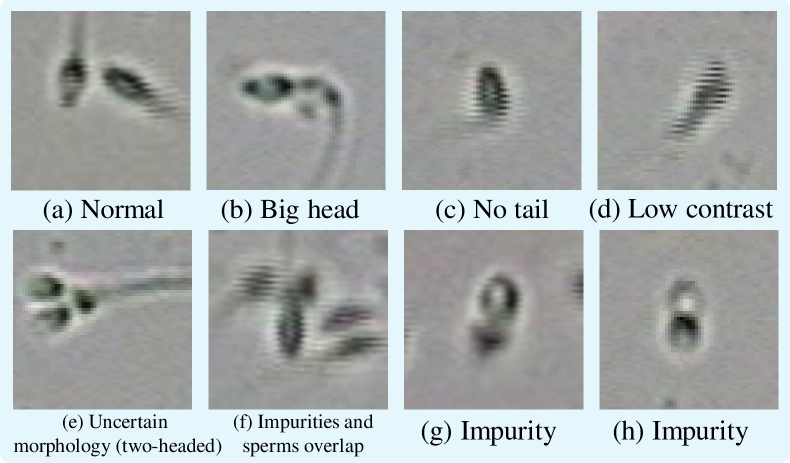
Figure 1: Examples of different sperm types.

So far, the detection of sperms and impurities still largely relies on traditional image processing techniques [5, 6, 7, 8, 9] which primarily include threshold-based methods, shape fitting methods, and filtering methods. i) Threshold-based methods find the best threshold to binarize an image [10]. In [5], sperm detection is accomplished by sequentially performing contrast enhancement, grayscale conversion, background identification, and background subtraction operations on the image, and finally binarizing the image using maximum entropy as the best threshold. In [6], sperm detection is performed by sequentially performing Gaussian filtering and Laplacian-of-Gaussian (LoG) filtering operations on the image, and finally binarizing the image using the Ostu [11] threshold method. ii) The shape-fitting methods use a polygon to fit the object. In [7] and [9], a rectangular area and an ellipse similar to the shape of the sperm are used to fit sperms, respectively, and then the parameters of the rectangle and ellipse are used to describe the position of the sperm, respectively. iii) The filtering methods filter the image with a suitable filter to separate the object and the background. In [12], morphological filters are used to isolate sperm cells. First, sperm cells are separated from other debris by filtering the image sequence according to a top-hat operation using appropriate structuring elements, followed by an open filter to reduce the remaining noisy objects smaller than the sperm head. However, these traditional detection methods only yield limited performance and often require manual intervention. Consequently, it not only escalates the time cost but also unavoidably injects the subjective bias into a CASA system.

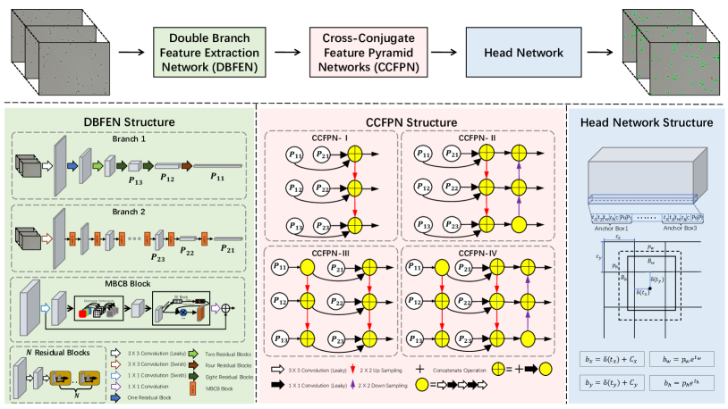
Figure 2: The architecture of ACTIVE. From the left to the right are the DBFEN, CCFPN and head network structures.

In recent years, deep learning (DL), a representative data-driven approach, has been dominating numerous imaging applications [13], ranging from low-level to high-level tasks. It has been widely confirmed by practitioners that provided well-curated big data and sufficient computing power, deep learning can deliver satisfactory results due to its strong feature extraction power. With the advent of the deep learning era, many excellent object detection models have been proposed, such as Region-based Convolutional Neural Networks (RCNNs) [14, 15], You Only Look Once (YOLO) series [16, 17], Single Shot Multibox Detector (SSD) [18], and Efficientdet [19]. It has been shown that CNNs can outperform classical image processing algorithms in most object detection tasks [20]. However, deep learning-based methods were unfortunately little explored in the field of sperm detection and analysis [4]. In [21], a CNN network was designed to detect sperm, but there is a drawback in choosing the best threshold in the whole process. [22] was mainly concerned with the sperm classification task. In [23], a deep learning method called TOD-CNN was proposed which obtains good detection performance for sperms but fails impurities.

In this investigation, we propose a deep learning model, referred to as ACTIVE (A Deep Model for Sperm DeteCTIon in Microscopic VidEos). As Fig. 2 shows, given the sperm videos from the Sperm Videos and Images Analysis (SVIA) dataset [24], the proposed ACTIVE framework consists of three main parts: Double Branch Feature Extraction Network (DBFEN), Cross-Conjugate Feature Pyramid Networks (CCFPN), and predicted network. Two branches of DBFEN respectively use residual structures and mobile inverted bottleneck convolution block to extract features and enhance the generalization ability, while DBFEN can fuse abundant features of different resolutions to facilitate the detection of tiny sperms and impurities. The contributions of this paper are as follows:

• We propose a double-branch deep learning framework, namely ACTIVE, which facilitates feature extraction and utilizes a series of novel structures to perform the feature fusion. Our work is the pioneer of introducing deep learning approaches into the field of computer-aided semen analysis.

• Experiments demonstrate that our proposed ACTIVE can overcome the difficulties of the sperm and impurity detection such as tiny size and indefinite morphology to achieve the state-of-the-art performance.

II Methodology

II-A Double Branch Feature Extraction Network (DBFEN)

DBFEN uses two branches to extract effective features of sperm microscopic images, which pays more attention to the features with the largest amount of information. Meanwhile, it also supports increasing the depth of the network to extract more features to further improve the detection performance.

Branch 1 mainly uses residual structures to extract features and facilitate training. The residual structure consists of a $3\times 3$ convolutional filter with a step size of 2, a $1\times 1$ convolutional filter, and a $3\times 3$ convolutional filter. The $3\times 3$ convolutional filter with the step size of 2 can help the network to compress the width and height of feature maps, which is similar to the function of the pooling operation. The feature map generated by the $3\times 3$ convolutional filter with the step size of 2 is concatenated with the feature map generated by the $3\times 3$ convolutional filter. This concatenation can avoid the gradient vanishment problem, thereby allowing a deep structure.

Branch 2 mainly uses Mobile inverted Bottleneck Convolution Block (MBCB) [19] to extract features. It first employs a 1 $\times$ 1 convolution filter on the input and changes the output channel dimension by the expansion ratio (if the expansion ratio is $k$, the channel dimension will grow by $k$ times. If the expansion ratio is 1, the 1 $\times$ 1 convolution filter and subsequent batch normalization and activation functions will be directly omitted). Second, the 3 $\times$ 3 depth-wise convolution filter is applied. Then, the Squeeze and Excitation (SE) block is introduced to this branch. After that, to recover the original channel dimension, a 1 $\times$ 1 convolution filter is used. Finally, the drop operation and skip connection are introduced to copy the input feature map to the end of the structure [25], which can discard the weights between hidden layers according to a fixed probability instead of simply discarding hidden nodes and sample the weights of each node with a Gaussian distribution in the testing stage to effectively solve problems caused by model quantization [26].

When we use the repeated MBCB, this block will perform connection deactivation and input jump connection. Connection deactivation is an operation similar to random deactivation, and the skip connection is added to combine the feature maps at the earlier and later parts of the model. Therefore, we can use different numbers of MBCB to eliminate the dependence between neural units and enhance the generalization ability [19]. Simultaneously, the SE Block [27] utilizes the attention mechanism or gate control on the channel dimension, which allows the model to pay more attention to the channel features with the largest amount of information and suppress those unimportant channel features.

II-B Cross-Conjugate Feature Pyramid Networks (CCFPN)

To handle the detection of tiny sperms and impurities, abundant features of different resolutions obtained from the DBFEN are aggregated. Traditional top-down Feature Pyramid Networks (FPN) [28] is inherently limited by unidirectional information flow, while Pyramid Attention Networks (PANet) [29] adds an additional bottom-up path. Based on FPN and PANet, as shown in Fig. 2, we propose CCFPN to fuse multi-resolution features: $\mathbf{P}^{\rm out}=\textit{f}(\mathbf{P}^{\rm in})$, where $\mathbf{P}^{\rm in}=(P_{11}^{\rm in},...,P_{ij}^{\rm in},...)$ is a list of multi-scale features, and $P_{ij}^{\rm in}$ represents the input feature of the preceding layer $j$ of the $i$-th branch. CCFPN has four variants:

$$\left\{\leavevmode\resizebox{399.2946pt}{}{$\begin{aligned} &{\rm CCFPN_{I}}(P_{1}^{\rm out})={\rm Conv}(P_{11}^{\rm in}+P_{21}^{\rm in})&\\ &{\rm CCFPN_{I}}(P_{2}^{\rm out})={\rm Conv}(P_{12}^{\rm in}+P_{22}^{\rm in}+{\rm Up}({\rm CCFPN_{I}}(P_{1}^{out})))&\\ &{\rm CCFPN_{I}}(P_{3}^{\rm out})={\rm Conv}(P_{13}^{\rm in}+P_{23}^{\rm in}+{\rm Up}({\rm CCFPN_{I}}(P_{2}^{\rm out})))&\end{aligned}$}\right.$$ (1)

$$\left\{\leavevmode\resizebox{399.2946pt}{}{$\begin{aligned} &{\rm CCFPN_{II}}(P_{1}^{\rm out})={\rm Conv}({\rm CCFPN_{I}}(P_{1}^{\rm out})+{\rm Down}({\rm CCFPN_{II}}(P_{2}^{\rm out})))&\\ &{\rm CCFPN_{II}}(P_{2}^{\rm out})={\rm Conv}({\rm CCFPN_{I}}(P_{2}^{\rm out})+{\rm Down}({\rm CCFPN_{II}}(P_{3}^{\rm out})))&\\ &{\rm CCFPN_{II}}(P_{3}^{\rm out})={\rm Conv}({\rm CCFPN_{I}}(P_{3}^{\rm out}))&\end{aligned}$}\right.$$ (2)

$$\left\{\leavevmode\resizebox{399.2946pt}{}{$\begin{aligned} &{\rm CCFPN_{III}}(P_{11}^{\rm in})={\rm Conv}(P_{11}^{\rm in})&\\ &{\rm CCFPN_{III}}(P_{12}^{\rm in})={\rm Conv}(P_{12}^{\rm in}+{\rm Up}({\rm CCFPN_{III}}(P_{11}^{\rm in})))&\\ &{\rm CCFPN_{III}}(P_{13}^{\rm in})={\rm Conv}(P_{12}^{\rm in}+{\rm Up}(\rm CCFPN_{III}(P_{12}^{in})))&\\ &{\rm CCFPN_{III}}(P_{1}^{\rm out})={\rm Conv}({\rm CCFPN_{III}}(P_{11}^{\rm in})+P_{21}^{\rm in})&\\ &{\rm CCFPN_{III}}(P_{2}^{\rm out})={\rm Conv}({\rm CCFPN_{III}}(P_{12}^{\rm in})+P_{22}^{\rm in}+{\rm Up}({\rm CCFPN_{III}}(P_{1}^{\rm out})))&\\ &{\rm CCFPN_{III}}(P_{3}^{\rm out})={\rm Conv}({\rm CCFPN_{III}}(P_{13}^{\rm in})+P_{23}^{\rm in}+{\rm Up}({\rm CCFPN_{III}}(P_{2}^{\rm out})))&\end{aligned}$}\right.$$ (3)

$$\left\{\leavevmode\resizebox{399.2946pt}{}{$\begin{aligned} &{\rm CCFPN_{IV}}(P_{1}^{\rm out})={\rm Conv}({\rm CCFPN_{III}}(P_{1}^{\rm out})+{\rm Down}({\rm CCFPN_{IV}}(P_{2}^{\rm out})))&\\ &{\rm CCFPN_{IV}}(P_{2}^{\rm out})={\rm Conv}({\rm CCFPN_{III}}(P_{2}^{\rm out})+{\rm Down}({\rm CCFPN_{IV}}(P_{3}^{\rm out})))&\\ &{\rm CCFPN_{IV}}(P_{3}^{\rm out})={\rm Conv}({\rm CCFPN_{III}}(P_{3}^{\rm out}))&\end{aligned}$}\right.$$ (4)

In Eqs. 1-4, we unify the outputs of CCFPN-I $\sim$ CCFPN-IV in Fig. 2 from top, middle to bottom into $(P_{1}^{\rm out},P_{2}^{\rm out},P_{3}^{\rm out})$, and add prefix ${\rm CCFPN_{I}}$ $\sim$ ${\rm CCFPN_{IV}}$ to distinguish different CCFPN variants. For example, in Fig. 2, ${\rm CCFPN_{I}}(P_{1}^{\rm out})$ represents the top output in CCFPN-I, ${\rm CCFPN_{II}}(P_{2}^{\rm out})$ represents the middle output in CCFPN-II, and ${\rm CCFPN_{III}}(P_{3}^{\rm out})$ represents the bottom output in CCFPN-III. In Eqs. 1-4, the up and Down arrows represent an up-sampling and down-sampling operation for resolution matching, respectively, and Conv is a convolution operation for feature processing.

Unlike other FPNs [28, 29, 19], CCFPN uses more multi-scale input features $\mathbf{P}^{\rm in}$ in a novel manner. From Fig. 2 and formulas (Eqs. 1-4), it can be found that CCFPN-I and CCFPN-III integrate more low-level detail information and more high-level semantic information, increasing the receptive field of the low-level, so that the low-level can obtain more context information when doing tiny object detection. CCFPN-II and CCFPN-IV following CCFPN-I and CCFPN-III can shorten the information transmission path and use the accurate positioning information of low-level features. To sum up, in detecting sperms and impurities, CCFPN makes use of more contextual information and accurate positioning information about sperms and impurities to improve the detection rate.

II-C Head Network

Three bounding boxes are predicted for each unit in the output feature map [16]. For each bounding box, seven coordinates ($t_{x}$, $t_{y}$, $t_{w}$, $t_{h}$, $C$, $P_{0}$, and $P_{1}$) are predicted, $t_{x}$ and $t_{y}$ are the offsets gained by the ACTIVE through sigmoid, and $t_{w}$ and $t_{h}$ are the scaling factors with the a priori box, $C$ is the confidence level about whether an object exists in the bounding box, $P_{0}$ and $P_{1}$ represent the probability of sperms and impurities in the bounding box. For each cell, assume that the offset from the upper left corner of the image is ($C_{x}$, $C_{y}$), and the width and height of the corresponding a priori box are $P_{w}$ and $P_{h}$. The calculation method of the center coordinates ($b_{x}$ and $b_{y}$), width ($b_{w}$) and height ($b_{h}$) of the prediction box is shown in Fig 2. Multi-label classification is applied to predict the categories in each bounding box. In addition, because the head network adopts the dense prediction method, a non-maximum suppression method based on distance intersection on union set [30] is used to remove the boundary boxes with high overlap in the network output results.

III Experiment

III-A Experimental Settings

III-A1 DataSet

In our work, our data are from subset-A of the SVIA dataset, a disclosed large-scale dataset for sperm detection [24]. Subset-A contains 101 videos and 3622 sperm images (frames). We first group the sperm videos into the training, validation, and test sets with a ratio of 6:2:2. Then we use the images obtained by framing these videos. The exemplary images from SVIA Subset-A are shown in Fig. 3.

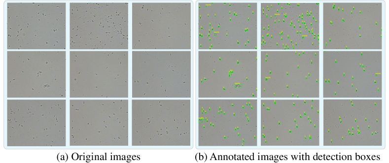
Figure 3: Examples of the images in SVIA Subset-A.

III-A2 Implementation Details

The experiment is conducted in Python 3.6.16 and Pytorch 1.7.1 in Windows 10. Our workstation is with Intel(R) Core(TM) i7-10700 CPU with 3.00GHz, 32GB RAM, and NVIDIA GEFORCE RTX 3060 12GB. For location and classification, we use the IOU function (location loss function) and the binary cross-entropy function (confidence and classification loss function) [16]. For optimization, we use Adam optimizer with default parameters for the whole experiment. For the other hyperparameters, the freeze training strategy is used in the experiments, when freezing partial layers and freezing no layers, the batch size is set to 4 and 2, the epoch number is 50 and 100, and the learning rate is set to $1\times 10^{-3}$ and $1\times 10^{-4}$, respectively. The input images are resized to 416 $\times$ 416 pixels.

III-A3 Evaluation Metrics

${\rm AP}_{50}$ is used as a metric for performance evaluation. ${\rm AP}_{50}$ represents the value of AP when IOU is 0.5. The definitions of AP and IOU are:

$$\footnotesize\lvert\{\begin{aligned} &{\rm Precision}=\frac{{\rm TP}}{{\rm TP}+{\rm FP}},~{}~{}~{}~{}~{}~{}~{}~{}~{}~{}~{}~{}~{}{\rm Recall}=\frac{{\rm TP}}{{\rm TP}+{\rm FN}},\\ &{\rm AP}=\frac{\sum_{i=1}^{N}\rm Precision_{\rm{max}}(\textit{i})}{\rm Number~{}of~{}Annotations},~{}{\rm IOU}=\frac{\rm G_{True}\bigcap G_{Pred}}{{\rm G_{True}\bigcup G_{Pred}}},&\\ \end{aligned}\rvert$$ (5)

where TP, TN, FP, and FN represent True Positive, True Negative, False Positive, and False Negative, $N$ denotes the number of detected objects. $G_{\rm True}$ and $G_{\rm Pred}$ represent the areas of the real box and the prediction box, respectively.

III-B Evaluation of Sperm and Impurity Detection Methods

To demonstrate the effectiveness of the ACTIVE models for the detection of sperms and impurities in sperm microscopic images, we compare our model with the aforementioned deep learning detection methods including one-stage object detection (Faster-RCNN) and two-stage object detection (SSD, EfficientDet-D2 and YOLO-V3/V4). The experiments validate that our proposed model can outperform the existing advanced object detection models by a large margin.

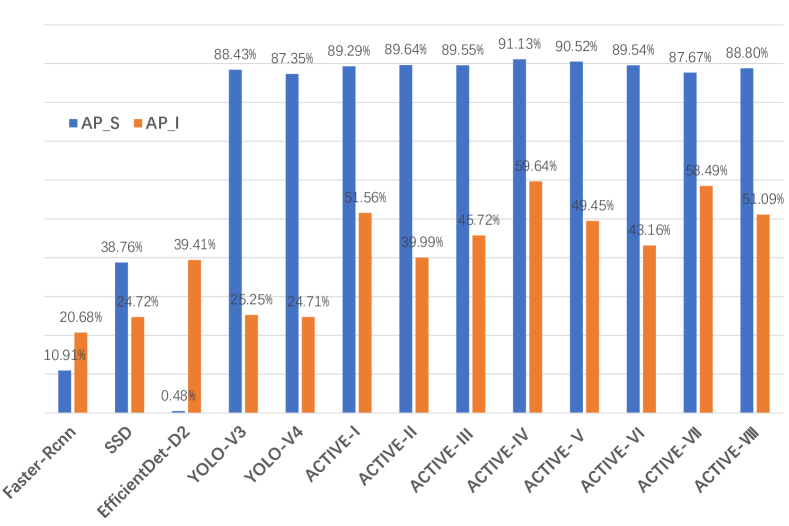
Figure 4: The AP of some deep learning detection methods and ACTIVE family models. AP_I and AP_S represent AP of impurity and AP of sperm, respectively. The highest performance of our proposed models obtains 91.13% and 59.64% of ${\rm AP}_{50}$ of the sperm and impurity detection with ACTIVE-IV.

$\bullet$ Evaluation of the sperm and impurity detection performance. Fig. 4 shows the APs of all object detection methods. It can be seen that YOLO-V3 has good performance in sperm detection, but poor performance in impurity detection. EfficientDet-D2 performs satisfactorily in impurity detection, but its performance in sperm detection is poor. Compared with its competitors, the ACTIVE model family not only improves the performance of sperm detection but also greatly improves the performance of impurity detection. In particular, compared with YOLO-V3, which has high sperm detection performance, the AP of sperm detection of ACTIVE-V is increased by 2.7%, while the AP of impurity detection of ACTIVE-V is increased by 34.39%. Compared with EfficientDet-D2 with high impurity detection performance, the AP of sperm detection of ACTIVE-V is incredibly increased by 90.09%, while the AP of impurity detection of ACTIVE-V is also greatly increased by 20.23%. What’s more, to visually appreciate the superior performance of ACTIVE, the detection results generated by the existing models and ACTIVE-IV model are in Fig. 5, wherein the “Sperm-normal” scenes (healthy) and the “Sperm-lack” scenes (oligospermia), the number of detection and correct detection cases of ACTIVE-IV are the best, far higher than other deep models. In Supplementary Materials, we show that how our model can assist doctors in clinical sperm diagnosis better than SSD and YOLO-v4.

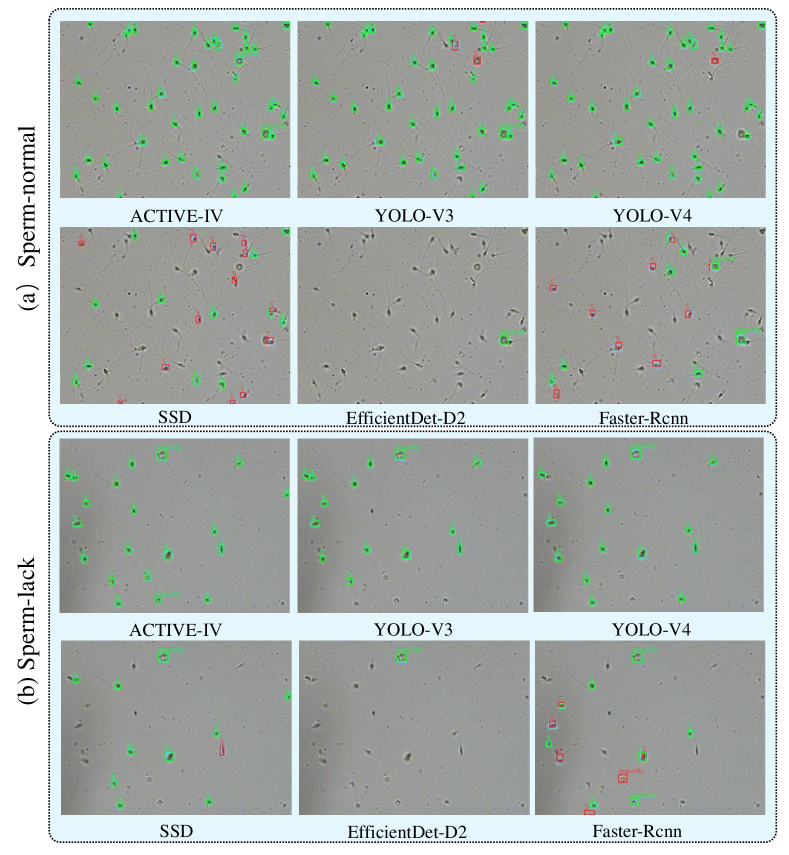
Figure 5: Comparison of ACTIVE-IV with YOLO-V4, YOLO-V3, SSD, EfficientDet-D2 and Faster-RCNN. The blue, green, and red boxes represent the GT, the correctly detected objects, and the incorrectly detected objects, respectively.

$\bullet$ Cross-validation experiment. To evaluate the reliability and accuracy of ACTIVE, we conduct five-cross validation. The experimental results are shown in Tab. I. It can be found that EfficinetDet-D2 obtains the best impurity detection performance and ACTIVE-IV achieves the best sperm detection performance. Compared with EfficinetDet-D2, the AP value of impurities in ACTIVE series models is decreased by about 10 %, but the AP value of sperm is increased by about 70%. Compared with YOLO-V3/V4 with competitive sperm detection performance, the AP value of sperm in ACTIVE series models is increased by about 2%, while the AP value of impurities is increased by about 10%. In general, ACTIVE series models are superior to existing models in sperms and impurities detection. In Supplementary Materials, we also compare the memory, training cost, and frames per second (FPS) of different models.

TABLE I:
The detection results of the five-fold cross-validation experiments. ( AP_I and AP_S respectively represent the average value of AP of sperms and impurities. )

Model	AP_I (%)	AP_S (%)
Faster-Rcnn	39.05	19.48
SSD	3.59	40.95
EfficientDet-D2	48.8	22.04
YOLO-V3	27.97	89.64
YOLO-V4	28.75	87.92
ACTIVE-I	41.03	90.24
ACTIVE-II	35.18	90.72
ACTIVE-III	39.55	90.93
ACTIVE-IV	37.18	91.23
ACTIVE-V	36.34	91.03
ACTIVE-VI	32.39	90.61
ACTIVE-VII	36.39	90.43
ACTIVE-VIII	33.24	90.18

$\bullet$ Ablation experiment. To evaluate the effectiveness of our proposed double branches in the ACTIVE framework, we conduct ablation experiments, as shown in Tab. II. Compared with only using branch 1, the AP value of sperm and impurity using a double branch feature extraction network is increased by 0.85% and 26.31%, respectively, and the gain is substantial. Compared with only using branch 2, the AP value of sperm and impurities using a double branch feature extraction network is increased by 12.15% and 88.81%, respectively. Therefore, the DBFEN effectively improves the detection performance of sperms and impurities. This network is effective for the detection of sperms and impurities.

TABLE II:
Results of the ablation experiments. (DBFEN1 and DBFEN2 represent branch 1 and branch 2 in the DBFEN network respectively. ✓means it is used.)

DBFEN1	DBFEN2	Category	AP (%)
✓		Impurity	25.25
		Sperm	88.43
	✓	Impurity	39.41
		Sperm	0.48
✓	✓	Impurity	51.56
		Sperm	89.29

IV Discussion

Here, we discuss the limitations of ACTIVE-(I-VIII) models for future improvement. As shown in Fig. LABEL:FIG:7, there exist three kinds of imperfections in ACTIVE: overlooked, misclassified, and incomplete detection objects.

i) Fig. LABEL:FIG:7(a) suggests that the reason why models overlook sperms and impurities is because of the following cases: low-resolution, residual shadow, and too tiny objects. The low-resolution object is due to the low quality of the data set, which may lose valuable information. The residual shadow object is generated because of the too fast-moving objects during the collection of sperm and impurity data, which is unavoidable but causes a streaked morphology. In addition, some objects are too tiny to be leveraged.

ii) The incorrect detection of objects, as shown in Fig. LABEL:FIG:7(b), is mainly due to the identical sperm and impurity, overlapping of sperm and impurity positions, and the edge of the object position. It is challenging to explore the complete information for sperms and impurities that appear at the edges. Thus, these sperms and impurities are generally missed in the detection. Furthermore, to ensure the reliability of the annotated information, the dataset is only annotated with sperms and impurities that are not disputed. Several sperms and impurities may be deeply located in the wet film of semen. However, their microscopic images are not precise, and it is difficult to distinguish whether they are sperms or impurities, so they are not annotated in the dataset. Unannotated sperms and impurities can be detected, leading to false detection.

iii) As shown in Fig. LABEL:FIG:7(c), the incomplete detection is because of uncertain morphology (double-headed sperm, large-headed sperm, etc.), low-resolution object, residual shadow object, overlapping of the sperm and impurity positions (a two-head sperm’s features are identical to impurities or sperms overlapping), and the edge of the object position.

V Conclusion and Future Work

In this paper, we propose the model ACTIVE for the object detection task of microscopic sperm images using the DBFEN and the CCFPN. The proposed ACTIVE model aided by CCFPN has established the state-of-the-art sperm and impurity detection performance on the SVIA dataset. In the future, we plan to increase the number of annotations of microscopic sperm images in the SVIA dataset and optimize the memory cost of ACTIVE. Also, we will consider the use of the image super-resolution technique in microscopic sperm images to enhance sperm detection.

References

- [1] N. Maharlouei, B. Morshed Behbahani, L. Doryanizadeh, and M. Kazemi, “Prevalence and pattern of infertility in iran: A systematic review and meta-analysis study,” Women’s Health Bulletin, vol. 17, no. 2, pp. 63–71, 2021.
- [2] G. Fallara, W. Cazzaniga, L. Boeri, P. Capogrosso, L. Candela, E. Pozzi, F. Belladelli, N. Schifano, E. Ventimiglia, C. Abbate et al., “Male factor infertility trends throughout the last 10 years: Report from a tertiary-referral academic andrology centre,” Andrology, vol. 9, no. 2, pp. 610–617, 2021.
- [3] N. Kumar and A. K. Singh, “Trends of male factor infertility, an important cause of infertility: A review of literature,” Journal of human reproductive sciences, vol. 8, no. 4, p. 191, 2015.
- [4] W. Zhao, P. Ma, C. Li, X. Bu, S. Zou, T. Jang, and M. Grzegorzek, “A survey of semen quality evaluation in microscopic videos using computer assisted sperm analysis,” arXiv: 2202.07820, 2022.
- [5] M. Elsayed, T. M. El-Sherry, and M. Abdelgawad, “Development of computer-assisted sperm analysis plugin for analyzing sperm motion in microfluidic environments using image-j,” Theriogenology, vol. 84, no. 8, pp. 1367–1377, 2015.
- [6] L. F. Urbano, P. Masson, M. VerMilyea, and M. Kam, “Automatic tracking and motility analysis of human sperm in time-lapse images,” IEEE transactions on medical imaging, vol. 36, no. 3, pp. 792–801, 2016.
- [7] X. Zhou and Y. Lu, “Efficient mean shift particle filter for sperm cells tracking,” in Proc. of ICCIS 2009, vol. 1, 2009, pp. 335–339.
- [8] X. Li, C. Li, F. Kulwa, M. M. Rahaman, W. Zhao, X. Wang, D. Xue, Y. Yao, Y. Cheng, J. Li et al., “Foldover features for dynamic object behaviour description in microscopic videos,” IEEE Access, vol. 8, pp. 114 519–114 540, 2020.
- [9] H.-F. Yang, X. Descombes, S. Prigent, G. Malandain, X. Druart, and F. Plouraboué, “Head tracking and flagellum tracing for sperm motility analysis,” in Proc. of ISBI 2014, 2014, pp. 310–313.
- [10] K. Bhargavi and S. Jyothi, “A survey on threshold based segmentation technique in image processing,” International Journal of Innovative Research and Development, vol. 3, no. 12, pp. 234–239, 2014.
- [11] N. Otsu, “A threshold selection method from gray-level histograms,” IEEE transactions on systems, man, and cybernetics, vol. 9, no. 1, pp. 62–66, 1979.
- [12] M. R. Ravanfar and M. H. Moradi, “Low contrast sperm detection and tracking by watershed algorithm and particle filter,” in Proc. of ICBME 2011, 2011, pp. 260–263.
- [13] D. Wang, F. Fan, Z. Wu, R. Liu, F. Wang, and H. Yu, “Ctformer: Convolution-free token2token dilated vision transformer for low-dose ct denoising,” arXiv preprint arXiv:2202.13517, 2022.
- [14] S. Ren, K. He, R. Girshick, and J. Sun, “Faster r-cnn: Towards real-time object detection with region proposal networks,” vol. 28, 2015.
- [15] K. He, G. Gkioxari, P. Dollár, and R. Girshick, “Mask r-cnn,” in Proc. of ICCV 2017, 2017, pp. 2961–2969.
- [16] J. Redmon and A. Farhadi, “Yolov3: An incremental improvement,” in Proc. of CVPR 2018, 2018, pp. 1804–02.
- [17] A. Bochkovskiy, C.-Y. Wang, and H.-Y. M. Liao, “Yolov4: Optimal speed and accuracy of object detection,” arXiv: 2004.10934, 2020.
- [18] W. Liu, D. Anguelov, D. Erhan, C. Szegedy, S. Reed, C.-Y. Fu, and A. C. Berg, “Ssd: Single shot multibox detector,” in Proc. of ECCV 2016, 2016, pp. 21–37.
- [19] M. Tan, R. Pang, and Q. V. Le, “Efficientdet: Scalable and efficient object detection,” in Proc. of CVPR 2020, 2020, pp. 10 781–10 790.
- [20] Z. Zou, Z. Shi, Y. Guo, and J. Ye, “Object detection in 20 years: A survey,” arXiv: 1905.05055, 2019.
- [21] M. S. Nissen, O. Krause, K. Almstrup, S. Kjærulff, T. T. Nielsen, and M. Nielsen, “Convolutional neural networks for segmentation and object detection of human semen,” in Proc. of SCIA 2017, 2017, pp. 397–406.
- [22] D. Somasundaram and M. Nirmala, “Faster region convolutional neural network and semen tracking algorithm for sperm analysis,” Computer Methods and Programs in Biomedicine, vol. 200, p. 105918, 2021.
- [23] S. Zou, C. Li, H. Sun, P. Xu, J. Zhang, P. Ma, Y. Yao, X. Huang, and M. Grzegorzek, “Tod-cnn: An effective convolutional neural network for tiny object detection in sperm videos,” Computers in Biology and Medicine, p. 105543, 2022.
- [24] A. Chen, C. Li, S. Zou, M. M. Rahaman, Y. Yao, H. Chen, H. Yang, P. Zhao, W. Hu, W. Liu et al., “Svia dataset: A new dataset of microscopic videos and images for computer-aided sperm analysis,” Biocybernetics and Biomedical Engineering, 2022.
- [25] G. Huang, Y. Sun, Z. Liu, D. Sedra, and K. Q. Weinberger, “Deep networks with stochastic depth,” in Proc. of ECCV 2016. Springer, 2016, pp. 646–661.
- [26] A. Mobiny, P. Yuan, S. K. Moulik, N. Garg, C. C. Wu, and H. Van Nguyen, “Dropconnect is effective in modeling uncertainty of bayesian deep networks,” Scientific reports, vol. 11, no. 1, pp. 1–14, 2021.
- [27] J. Hu, L. Shen, and G. Sun, “Squeeze-and-excitation networks,” in Proc. of CVPR 2018, 2018, pp. 7132–7141.
- [28] T.-Y. Lin, P. Dollár, R. Girshick, K. He, B. Hariharan, and S. Belongie, “Feature pyramid networks for object detection,” in Proc. of CVPR 2017, 2017, pp. 2117–2125.
- [29] S. Liu, L. Qi, H. Qin, J. Shi, and J. Jia, “Path aggregation network for instance segmentation,” in Proc. of CVPR 2018, 2018, pp. 8759–8768.
- [30] Z. Zheng, P. Wang, W. Liu, J. Li, R. Ye, and D. Ren, “Distance-iou loss: Faster and better learning for bounding box regression,” in Proc. of AAAI 2020, vol. 34, no. 07, 2020, pp. 12 993–13 000.