Object Detection performance variation on compressed satellite image datasets with iquaflow

Abstract

Increasing the performance of predictive models on images has been in the focus of many research projects lately.However, studies about the resilience of these models when they are trained on image datasets that suffer modifications altering their original quality are less common, even though their implications are often encountered in the industry [1],[2],[3]. A good example of that is with earth observation satellites that are capturing many images. The energy and time of connection to the earth of an orbiting satellite are limited and must be carefully used. An approach to mitigate that is to compress the images on board before downloading. The compression can be regulated depending on the intended usage of the image and the requirements of this application. We present a new software tool with the name iquaflow that is designed to study image quality and model performance variation given an alteration of the image dataset. Furthermore, we do a showcase study about oriented object detection models adoption on a public image dataset DOTA [4] given different compression levels. The optimal compression point is found and the usefulness of iquaflow becomes evident.

Keywords vision  $\cdot$ object detection  $\cdot$ oriented bounding box  $\cdot$ deep learning  $\cdot$ compression  $\cdot$ lossy compression  $\cdot$ onboard compression  $\cdot$ earth observation  $\cdot$ image quality

1 Introduction

Predictive models that use images as inputs are constrained to any image alteration that can degrade the optimal performance of these models. Sometimes the degree of modification on the images can be regulated. A good example is when images are compressed before being sent to the algorithm for prediction. In case of earth observation satellites, the high cost of downloading the images can be significantly reduced by compressing the images first. [1]. One approach is to make images smaller to reduce the costs of downloading to earth [5]. In this context, decision-makers need tools to study the optimal modification so that the performance of the predictive models is adequate despite the compression. iquaflow is a software tool that has been designed precisely to study image quality as well as the performance of models trained on top of provided datasets that are modified with any user-defined alteration. [1] studies object detection inference with compression algorithms based on decimation and scaling with interpolation in the context of earth observation from satellite applications. In the present work, the study is brought further with custom training for each level of compression, new kinds of compression, and new models of object detection that are suitable for oriented annotations as explained below.

1.1 Compression

Compression algorithms can be lossless or lossy [6]. The first kind performs an operation on the image that allows the recovery of the original image before it was compressed. The second kind, on the other hand, does an irreversible operation. Using a lossy compression algorithm, we can achieve a greater reduction in file sizes than with a lossless one. A simple straightforward technique for lossy compression can be the interpolation of an image to fewer pixels. Then a smaller image will have lost information and it will also be smaller in file size. In this study the JPEG compression is used as explained in section 2.2.

1.2 Object detection

A good example of predictive models on images is object detection (such as vehicles from aerial images). Most detectors such as Faster R-CNN [7], SSD [8] and YOLOv2, v3 [9] rely on a set of pre-defined anchors that consist in a small set of bounding boxes summarizing the most relevant geometric shapes covering relevant scale, aspect ratios and elongation directions. The idea is that any object can be associated with a specific anchor box without having to have a perfect fit.

However, the definition of this set of anchor boxes is a hyper-parameter that must be defined and has an effect on the detection performance. The models are, of course, sensitive to the sizes, aspect ratios, and a number of anchors defined in the set (see [7] and [10]).

Another aspect to consider is the number of stages. Detectors can be composed of multiple stages and each of them has a trained model that solves a specific task in the workflow. A typical case in an object detection problem is the Region Proposal Network which is responsible for the task of generating bounding box proposals. Examples of that are [11], [12] and [13]. One advantage of the multistage approach is that each step in the workflow can be easily defined and understood by human logic. In single-stage detectors, the logic can be difficult to interpret inside an end-to-end network solution.

Depending on the annotations one can use a model that predicts with horizontal bounding boxes (HBB) or oriented bounding boxes (OBB). One problem with HBB is distinguishing between overlapping instances of different objects. This is usually approached with the logic of Non-Maximum Suppression (NMS) that involves the measure of Intersection Over Union between different instances to asses the overlapping and whether or not candidate boxes belong to the same sample. This logic struggles when there are elongated objects that are diagonal and parallel to each other. In aerial images, these can be ships in a harbor or trucks in parking. One solution for this is to consider more complex geometries that have a better fit with the object. The simplest complexity, in this case, is to orient the bounding box.

The models used in this study are explained in section 2.3.

1.3 Iquaflow

Image quality can be often evaluated by the human eye. However, it is very challenging to define a numerical measurement for image quality. One of the reasons is that there are many aspects to consider such as the blur, the noise, the quality distribution along frequencies, etc. Moreover, image quality should be measured according to the particular application of the images being measured. Supervised super-resolution image prediction models are algorithms that translate an input image to a higher-resolution image that contains more pixels. These models are trained with a database containing pair samples of images with their respective higher resolution (also known as ground-truth or target images). In this context, the evaluation of quality will perform better by comparing the predicted image against the target image. These metrics are also known as similarity metrics and they include [14], [15], [16] and [17]. Another context is when images are used as inputs for other predictive models with the aim to collect information from them. It is the case of an image classifier or object detection. For this case, a suitable image quality evaluation method can be the performance of this model on the images. This is assuming that changes in the input image quality are affecting the performance of the prediction model. Again, this is a way to measure image quality that is adapted to the actual application of the image.

iquaflow[18] is a python package tool that measures image quality by using different approaches. Deterministic metrics include blind metrics which are measured directly on the image without comparing against a reference image or similarity metrics when they are measuring affinity against an ideal case. There are two metrics that have been designed for iquaflow which are implicit measurements of blur and noise levels. The first relies on edges found within the images and it measures the slope in the Relative Edge Response (RER) [19]. Then the second is based on homogeneous areas where the noise can be estimated (Signal to Noise ratio - SNR) [20]. The Quality Metric Regression Network (QMRNet)[21] has been designed, trained, and integrated into iquaflow. This is a classifier with small intervals that can predict quality parameters on images such as blur (measured as equivalent sigma from a gaussian bell), sharpness, pixel size and noise. Quality can also be measured by checking how predictive models trained on the image dataset are performing. A good example is the present study where object detection is trained on different quality datasets with different outcomes.

Apart from measuring image quality, iquaflow has a whole ecosystem that facilitates the design of new studies and experiment sets made of several training runs with variations. iquaflow wraps another open source tool named Mlflow that is used for machine learning experiment tracking. It will record the executions in a standard format so that they are later easily visualized and compared from Mlflow user interface tool in the browser. In iquaflow the user can add custom metrics and dataset modifiers that are easily integrated into a use case study.

2 Materials and Methods

The aim of the study is to measure the variation of the object detection algorithm’s performance on a given image dataset that is modified with various compression ratios. Our goal is to evaluate what is the maximum compression level that still allows for acceptable model performance. In this section, the compression algorithm is described, and the object detection model(s) that we considered, as well as the tool used for managing our experiments.

2.1 Data

Two different datasets are used to carry out two experiments. The first analysis is based on the airplanes dataset which consists of 998 images of 1024 × 1024 pixels from airport areas with a total of almost $17000$ annotated planes. These captures were made using NewSat Satellogic constellation ($1~{}\mathrm{m}$ GSD) and the annotations were made using Happyrobot platform. The training partition contained $13731$ annotations and the remaining were used for evaluation.

The second experiment was based on the public dataset DOTA [4]. It is a dataset for object detection in aerial images. The images are collected from different sensors the image sizes are ranging from $800~{}\times~{}800$ to $20000~{}\times~{}20000$ pixels and the pixel size varies from $0.3~{}\mathrm{m}$ to $2~{}\mathrm{m}$ resolution. DOTA has several versions and DOTA-v1.0 has been used in the present study which contains 15 common categories , $2806$ images and more than $188k$ object instances. The annotations are oriented bounding boxes which allows us to train both oriented (OBB) and horizontal bounding boxes (HBB) models. The proportions of the training set, validation set, and testing set in DOTA-v1.0 are $1/2$, $1/6$, and $1/3$ [4]. A disadvantage of this dataset is that the test set is not openly available, rather it is in a form of a remote service to query the predictions. This does not allow to alter the test on the same way the other partitions are modified in the present study. Because of that, 2 partitions are made from the validation set: half of is is used as actual validation and the other half for testing. Then the images are cropped to $1024~{}\times~{}1024$ with padding when necessary. After this operation the number of crops for the partitions train, validation and testing are respectively $9734$, $2670$ and $2627$.

2.2 Compression

In this study, JPEG compression [22] is used. It is a lossy form of compression based on the discrete cosine transform (DCT) that converts images into the frequency domain and discards high-frequency information by a quantization process. The degree of compression in JPEG can be adjusted: the greater the quality the bigger the file size. In the present study, the compression is set at different levels with the aim to find an optimal value with respect to the performance of predictive models trained on them. We used the JPEG compression from OpenCV [23] that can be regulated with the parameter CV_IMWRITE_JPEG_QUALITY which can vary from $0$ to $100$ (the higher is the better) with a default value of 95.

Figure 1 shows an example of the effect when compressing one of the images with JPEG method.

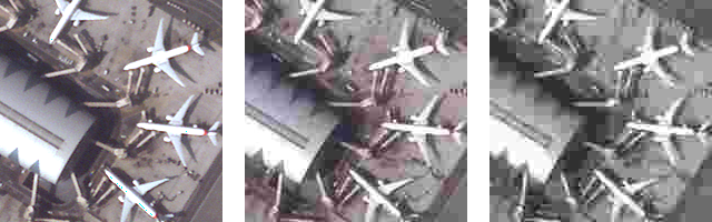
Figure 1: JPEG compression effects (original, JPG10,and JPG5 from left to right). This image is from the airplane dataset from Satellogic.

2.3 Object detection

The first experiment has HBB annotated objects and the model YOLOv5 [24] was used because of its fast training and implementation.

For the second experiment, two OBB models were used. The first was Oriented R-CNN which is a two-stage oriented detector that uses Region Proposal Network (oriented RPN) in the first stage in order to generate high-quality oriented proposals in a nearly cost-free manner [25].

Then the other model used was FCOS [26] which is originally designed for horizontal bounding boxes but it can be adapted with an added convolution layer channel on the top of the regression features that define the direction of the bounding box. Intersection Over Union is often used as a loss function in object detection. However, the IoU calculation between oriented boxes is complex and often not differentiable. There are rotated IoU that implements differentiable IoU calculation for oriented bounding boxes. In this case, the PolyIoULoss [27] between the OBB predictions and ground truths is used as a bounding box loss.

The performance of the detector is measured by calculating the average recall (AR) as well as the Mean Average Precision (mAP). AR is a ratio of correctly detected instances over the actual amount of objects. On the other hand, AP is defined with the same correctly detected instances over all the amount of detected cases (including wrong detection). The predicted bounding boxes do not have to have a perfect match with the ground truth. Because of that, the Intersection over Union (IoU) for each prediction and ground truth match candidate is measured to evaluate if they match. In which case it is considered a correct detection [28]. In this study, mAP is calculated by taking the mean AP over all classes and over a range of IoU thresholds.

2.4 Experiment management

The present study involves a workflow with multiple versions of the original dataset with the corresponding partitions for each altered version (train, validation and test) as well as many training experiment executions and tracking of results that must be organized correctly. All this can be managed easily with a typical iquaflow workflow as follows:

1. Optionally the user can start with a repository template of iquaflow use cases. This repository uses cookiecutter which is a python package tool for repository templates. By using this you can initialize a repository with the typical required files for a study in iquaflow.

2. The first step will be to set the modifications of the original dataset with different compression levels. This can be done with a list of Modifiers in iquaflow. There are some modifiers already available in iquaflow with performing specific alterations. However, one can set up a custom modifier by inheriting the DSModifier class of iquaflow. The list of modifiers will then be passed as an argument to the experiment setup.

3. Next step is to adapt the user training script to the iquaflow conventions. This is just to accept some input arguments such as the output path where the results are written. Optionally one can monitor in streaming the training by inputting additional arguments as explained in iquaflow’s guide.

4. All previous definitions are introduced in the experimental setup that can be executed afterward. The whole experiment will contain all runs which are the result of combining dataset modifications (the diverse compression levels) and the two different detectors that are used which will be defined as hyperparameter variations in the experiment setup.

5. The evaluation can be either done within the user’s custom training script or by using a Metric in iquaflow. Similar to Modifiers there are some specific Metrics already defined in iquaflow. Alternatively, the user can make a custom metric by inheriting the class Metric from iquaflow. The results can be collected from iquaflow or directly by raising an mlflow server which is a tool that is wrapped and used by iquaflow.

As you can see using iquaflow we can automate the compression algorithm on the data, run the user custom training script and evaluate a model. All the results are logged using mlflow and can be handily compared and visualized. iquaflow is the ideal tool for this purpose.

3 Results

The airplanes dataset from Satellogic has the unique category of planes. The image format is tiff and the original average image size is $3.204$Megabytes. The average recall (AR) is measured and the Mean Average Precision (mAP) is calculated over different Intersection Over Union (IoU) thresholds varying from $0.5$ to $0.95$ with a step of $0.05$ and average again for the final score. Table 1 contains the resultant metrics and Figure 2 shows performances (mAP) along different levels of compression.

Table 1: Performance results at different compression levels using the airplanes dataset and two YOLOv5 model sizes with different architecture complexities. The scores for the different models are expressed as Mean Average Precision (mAP) and Average Recall (AR) as expressed in the methodology section. The last column shows the equivalent average image size from the dataset given the level of compression used.

YOLOv5 NANO		YOLOv5 SMALL		size
AR	mAP	AR	mAP	Mb
0.898	0.669	0.922	0.714	2.051
0.899	0.666	0.919	0.709	1.428
0.892	0.663	0.917	0.708	1.256
0.888	0.657	0.916	0.703	0.988
0.872	0.636	0.891	0.675	0.874

Figure 2: Scatter plot that shows the performance of the models (mAP) evolution with different compression levels expressed as average image size of the files in the modified Satellogic’s airplanes dataset. Red with "x" and blue with "+" correspond to model size nano and small of YOLOv5 model respectively.

The DOTAv1.0 dataset has 15 categories and different metrics are measured for each class. The categories of ’plane’ and ’storage tank’ are performing the best whereas the categories ’bridge’ and ’soccer-ball-field’ are performing the worst. Table 2 summarizes the averaged metrics for each run by aggregating with the mean of all the categories. Following the same logic, Figure 3 charts the evolution of performance (mAP) along different levels of compression. The original average image size of the $1024~{}\times~{}1024$ crops without compression was $1.13$Megabytes.

Table 2: Performance results at different compression levels using the DOTA1.0 dataset and two OBB models. The scores for the different models are expressed as Mean Average Precision (mAP) and Average Recall (AR) as expressed in the methodology section. The last column shows the equivalent average image size from the dataset given the level of compression used.

FCOS		RCNN		size
AR	mAP	AR	mAP	Mb
0.869	0.688	0.806	0.662	0.332
0.856	0.677	0.812	0.658	0.321
0.865	0.692	0.813	0.668	0.311
0.861	0.679	0.812	0.666	0.313
0.861	0.679	0.810	0.663	0.305
0.861	0.685	0.806	0.668	0.273
0.849	0.677	0.811	0.669	0.245
0.856	0.675	0.804	0.659	0.226
0.847	0.673	0.800	0.660	0.209
0.846	0.666	0.798	0.658	0.191
0.835	0.651	0.785	0.649	0.171
0.831	0.643	0.785	0.636	0.138
0.799	0.598	0.741	0.588	0.097

The optimal compression ratio for the oriented-RCNN model seems to be around JPEG quality score of 70 which corresponds to an average image size of 0.245 Megabytes. This is because it corresponds to the minimum average file size that can be defined without lowering the performance. On the other hand, the adapted FCOS model seems to have an optimal around 80 for JPEG quality score which corresponds to an average image size of 0.273 Megabytes.

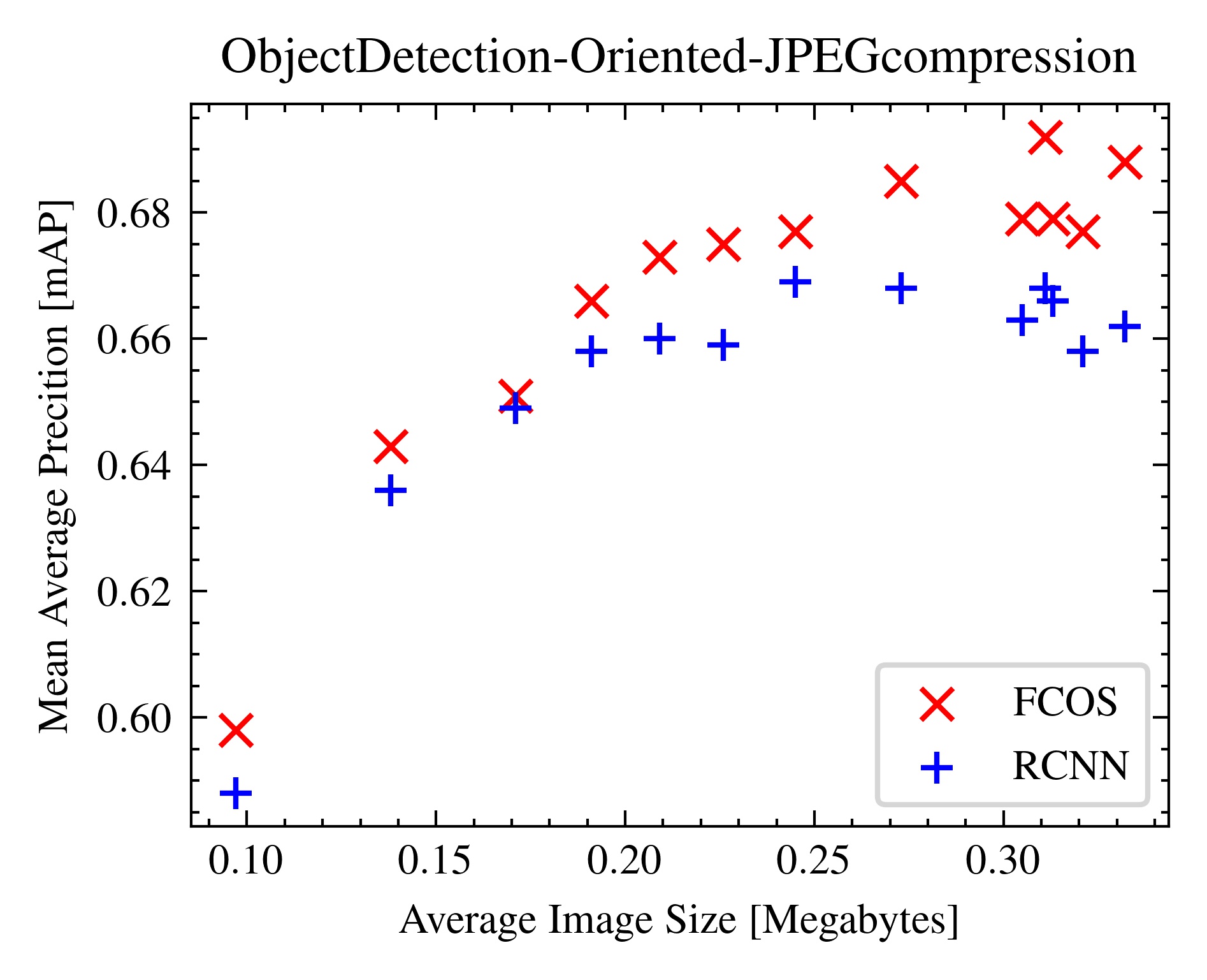
Figure 3: Scatter plot that shows the performance of the models (mAP) evolution with different compression levels expressed as average image size of the files using the DOTA1.0 dataset and two OBB models. Red dots correspond to the adapted FCOS model whereas blue dots are from the oriented RCNN model.

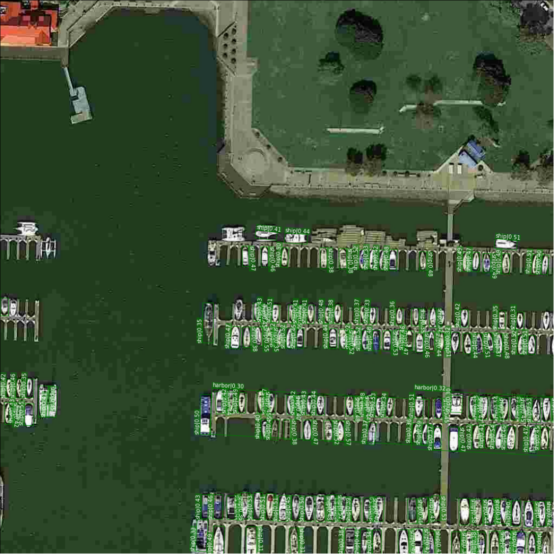
Figure 4: An example of prediction on an image with boats compressed with $CV\_JPEG\_QUALITY$ of $10$ which is equivalent to an average dataset image size of $0.097Mb$. The model used is adapted FCOS. The image belongs to the testing partition.

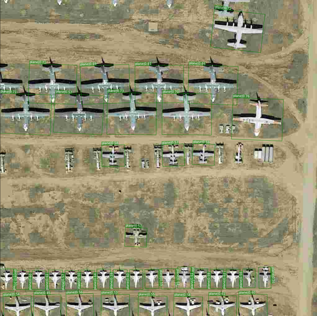
Figure 5: An example of prediction on an image with planes compressed with $CV\_JPEG\_QUALITY$ of $10$ which is equivalent to an average dataset image size of $0.097Mb$. The model used is adapted FCOS. The image belongs to the testing partition.

4 Conclusions

In the experiment with Satellogic’s airplanes dataset, the decrease in performance with compression is consistent for both models. The variations of mAP is small between the ranges of $0.15$ and $0.25$ average image size. The additional complexity of the Small model has a constant positive shift of $0.5$ in mAP with respect to the Nano model along all the analyzed compression rates.

In the context of the second experiment the adapted FCOS model seems to perform better than oriented RCNN because the AR and mAP are greater for all levels of compression. On the other hand, oriented-RCNN seems more resilient because the optimal compression ratio is higher than the optimal case for the other model. However, the degraded performance of FCOS model given the same compression setting as the optimal value for oriented-RCNN still offers higher performance. FCOS is also easier to implement because it is a single-stage detector that does not require setting anchors as hyperparameters. So far, given the data and context of the study, FCOS seems the best option.

Another interesting observation is the high resilience of the model for some specific applications. The figures 4 and 5 show a prediction with the FCOS model on an image with boats and airplanes respectively. Both of the images were set with a compression rate of $10$ for $CV\_JPEG\_QUALITY$ which is equivalent to an average dataset image size of $0.097Mb$. In the first image, $146$ ships were correctly detected (True positives), $9$ were wrongly detected (False positive) and $11$ ships were missed (False negative). In the other example all the planes (total amount: $39$) are correctly detected see 5 with no false positives or false negatives. This highlights the greater capacity of compressing images for usage such as the detection of airplanes over smaller or more difficult objects.

This study highlights the potential of iquaflow for decision-makers as well as researchers that want to study performance variation in an agile and ordered way. The key effort has been the development of the tool so that it facilitates further studies with the aim to scale it. The tool also allows for mitigating the uncertainty of image quality by using several strategies to measure that. This is helping also in studies that are exploring suitable solutions for satellite image Super Resolution.

References

- [1] Martina Lofqvist and José Cano. Optimizing data processing in space for object detection in satellite imagery, 2021.
- [2] Yong-Yeon Jo, Young Sang Choi, Hyun Woo Park, Jae Hyeok Lee, Hyojung Jung, Hyo-Eun Kim, Kyounglan Ko, Chan Wha Lee, Hyo Soung Cha, and Yul Hwangbo. Impact of image compression on deep learning-based mammogram classification. Scientific Reports, 11, 2021.
- [3] Kresimir Delac, Mislav Grgic, and Sonja Grgic. Effects of jpeg and jpeg2000 compression on face recognition. In Sameer Singh, Maneesha Singh, Chid Apte, and Petra Perner, editors, Pattern Recognition and Image Analysis, pages 136–145, Berlin, Heidelberg, 2005. Springer Berlin Heidelberg.
- [4] Gui-Song Xia, Xiang Bai, Jian Ding, Zhen Zhu, Serge Belongie, Jiebo Luo, Mihai Datcu, Marcello Pelillo, and Liangpei Zhang. Dota: A large-scale dataset for object detection in aerial images. In The IEEE Conference on Computer Vision and Pattern Recognition (CVPR), 5 2018.
- [5] Vinicius Alves de Oliveira, Marie Chabert, Thomas Oberlin, Charly Poulliat, Mickael Bruno, Christophe Latry, Mikael Carlavan, Simon Henrot, Frederic Falzon, and Roberto Camarero. Reduced-complexity end-to-end variational autoencoder for on board satellite image compression. Remote Sensing, 13(3), 2021.
- [6] Abir Jaafar Hussain, Ali Al-Fayadh, and Naeem Radi. Image compression techniques: A survey in lossless and lossy algorithms. Neurocomputing, 300:44–69, 2018.
- [7] Shaoqing Ren, Kaiming He, Ross Girshick, and Jian Sun. Faster R-CNN: Towards real-time object detection with region proposal networks. In Advances in Neural Information Processing Systems (NIPS), 2015.
- [8] Wei Liu, Dragomir Anguelov, Dumitru Erhan, Christian Szegedy, Scott E. Reed, Cheng-Yang Fu, and Alexander C. Berg. Ssd: Single shot multibox detector. In Bastian Leibe, Jiri Matas, Nicu Sebe, and Max Welling, editors, ECCV (1), volume 9905 of Lecture Notes in Computer Science, pages 21–37. Springer, 2016.
- [9] Joseph Redmon and Ali Farhadi. Yolov3: An incremental improvement, 2018. cite arxiv:1804.02767Comment: Tech Report.
- [10] Tsung-Yi Lin, Priya Goyal, Ross B. Girshick, Kaiming He, and Piotr Dollár. Focal loss for dense object detection. 2017 IEEE International Conference on Computer Vision (ICCV), pages 2999–3007, 2017.
- [11] Jian Ding, Nan Xue, Yang Long, Gui-Song Xia, and Qikai Lu. Learning roi transformer for detecting oriented objects in aerial images. CoRR, abs/1812.00155, 2018.
- [12] Yongchao Xu, Mingtao Fu, Qimeng Wang, Yukang Wang, Kai Chen, Gui-Song Xia, and Xiang Bai. Gliding vertex on the horizontal bounding box for multi-oriented object detection. IEEE Transactions on Pattern Analysis and Machine Intelligence, 43(4):1452–1459, 4 2021.
- [13] Xue Yang, Jirui Yang, Junchi Yan, Yue Zhang, Tengfei Zhang, Zhi Guo, Sun Xian, and Kun Fu. Scrdet: Towards more robust detection for small, cluttered and rotated objects, 2018.
- [14] Jim Nilsson and Tomas Akenine-Möller. Understanding ssim, 2020.
- [15] Richard Zhang, Phillip Isola, Alexei A. Efros, Eli Shechtman, and Oliver Wang. The unreasonable effectiveness of deep features as a perceptual metric, 2018.
- [16] Rafael Reisenhofer, Sebastian Bosse, Gitta Kutyniok, and Thomas Wiegand. A haar wavelet-based perceptual similarity index for image quality assessment. Signal Processing: Image Communication, 61:33–43, feb 2018.
- [17] Keyan Ding, Kede Ma, Shiqi Wang, and Eero P. Simoncelli. Image quality assessment: Unifying structure and texture similarity. IEEE Transactions on Pattern Analysis and Machine Intelligence, pages 1–1, 2020.
- [18] P. Gallés, K. Takats, M. Hernández-Cabronero, D. Berga, L. Pega, L. Riordan-Chen, C. Garcia, G. Becker, A. Garriga, A. Bukva, J. Serra-Sagristà, D. Vilaseca, and J. Marín. Iquaflow: A new framework to measure image quality, 2022.
- [19] Jon Leachtenauer, William Malila, John Irvine, Linda Colburn, and Nanette Salvaggio. General image-quality equation: Giqe. Applied optics, 36:8322–8, 12 1997.
- [20] Barry T. Bosworth, W. Robert Bernecky, James D. Nickila, Berhane Adal, and G. Clifford Carter. Estimating signal-to-noise ratio (snr). IEEE Journal of Oceanic Engineering, 33(4):414–418, 2008.
- [21] David Berga, Pau Gallés, Katalin Takáts, Eva Mohedano, Laura Riordan-Chen, Clara Garcia-Moll, David Vilaseca, and Javier Marín. Qmrnet: Quality metric regression for eo image quality assessment and super-resolution, 2022.
- [22] Gregory K. Wallace. The JPEG still picture compression standard. Communications of the ACM, 34:31–44, 4 1991.
- [23] G. Bradski. The OpenCV Library. Dr. Dobb’s Journal of Software Tools, 2000.
- [24] Glenn Jocher, Alex Stoken, Jirka Borovec, NanoCode012, Ayush Chaurasia, TaoXie, Liu Changyu, Abhiram V, Laughing, tkianai, yxNONG, Adam Hogan, lorenzomammana, AlexWang1900, Jan Hajek, Laurentiu Diaconu, Marc, Yonghye Kwon, oleg, wanghaoyang0106, Yann Defretin, Aditya Lohia, ml5ah, Ben Milanko, Benjamin Fineran, Daniel Khromov, Ding Yiwei, Doug, Durgesh, and Francisco Ingham. ultralytics/yolov5: v5.0 - YOLOv5-P6 1280 models, AWS, Supervise.ly and YouTube integrations. Zenodo, April 2021.
- [25] Xingxing Xie, Gong Cheng, Jiabao Wang, Xiwen Yao, and Junwei Han. Oriented r-cnn for object detection. In Proceedings of the IEEE/CVF International Conference on Computer Vision (ICCV), pages 3520–3529, 10 2021.
- [26] Zhi Tian, Chunhua Shen, Hao Chen, and Tong He. Fcos: A simple and strong anchor-free object detector. IEEE Transactions on Pattern Analysis and Machine Intelligence, 2021.
- [27] Jeffri M. Llerena, Luis Felipe Zeni, Lucas N. Kristen, and Claudio Jung. Gaussian bounding boxes and probabilistic intersection-over-union for object detection, 2021.
- [28] D. M. W. Powers. Evaluation: From precision, recall and f-measure to roc., informedness, markedness & correlation. Journal of Machine Learning Technologies, 2(1):37–63, 2011.