CEDAS: A Compressed Decentralized Stochastic Gradient Method with Improved Convergence

Abstract

In this paper, we consider solving the distributed optimization problem over a multi-agent network under the communication restricted setting. We study a compressed decentralized stochastic gradient method, termed “compressed exact diffusion with adaptive stepsizes (CEDAS)", and show the method asymptotically achieves comparable convergence rate as centralized SGD for both smooth strongly convex objective functions and smooth nonconvex objective functions under unbiased compression operators. In particular, to our knowledge, CEDAS enjoys so far the shortest transient time (with respect to the graph specifics) for achieving the convergence rate of centralized SGD, which behaves as $\mathcal{O}\left(nC^{3}/(1-\lambda_{2})^{2}\right)$ under smooth strongly convex objective functions, and $\mathcal{O}\left(n^{3}C^{6}/(1-\lambda_{2})^{4}\right)$ under smooth nonconvex objective functions, where $(1-\lambda_{2})$ denotes the spectral gap of the mixing matrix, and $C>0$ is the compression-related parameter. Numerical experiments further demonstrate the effectiveness of the proposed algorithm.

1 Introduction

In this paper, we consider solving the following distributed optimization problem by a group of agents $[n]:=\left\{1,2,\cdots,n\right\}$ connected over a network:

$$\min_{x\in\mathbb{R}^{p}}f(x)=\frac{1}{n}\sum_{i=1}^{n}f_{i}(x),$$ (1)

where $f_{i}$ is the local cost function known by agent $i$ only. Problem (1) appears naturally in many machine learning and signal processing problems, where each $f_{i}$ represents an expected or empirical risk function corresponding to the local dataset of agent $i$. Solving problem (1) in a decentralized manner over a multi-agent network has gained great interests in recent years, partly because decentralization helps relieve the high latency at the central server in a centralized computing architecture [26]. However, decentralized optimization algorithms may still suffer from the communication bottleneck under the huge size of modern machine learning models and/or limited bandwidth. For example, the gradients used for training LSTM models can be as large as $110.43$ MB [11].

Communication compression techniques, such as quantization [2, 4, 33] and sparsification [46, 39], are one of the most effective means for reducing the communication cost in distributed computation. The performance of several commonly used communication compression methods has been well studied under the centralized master-worker architecture, and the algorithms have been shown to enjoy comparable convergence rates with their non-compressed counterparts when equipped with various techniques such as error compensation [33, 31, 3, 39] and gradient difference compression [24]. It is thus natural to integrate decentralization and communication compression to benefit from both techniques. The work in [41] combined distributed stochastic gradient descent (DSGD) with quantization for the first time, followed by [12, 11] which extended the compressed DSGD method to fit a richer set of compression operators. The paper [22] equipped NIDS [18] with communication compression and demonstrated its linear convergence rate when the objective functions are smooth and strongly convex. More recently, the papers [20, 37] considered a class of linearly convergent decentralized gradient tracking method with communication compression that applies to general directed graphs; see also [54, 51] for more related works.

It is worth noting that introducing decentralization may slow down the algorithmic convergence as the network size grows when compared to the centralized master-worker architecture [29]. Therefore, an important question arises when considering decentralized optimization with communication compression, that is, can a compressed decentralized (stochastic) gradient method achieve similar convergence rate compared to its centralized counterpart? Such a question has been answered positively in [41] first with several works following [12, 11, 36, 35, 45]. However, these methods are all variants of DSGD which suffer from the data heterogeneity [27, 30, 19]. As a result, significant amount of transient times are often required for achieving comparable convergence rate with centralized SGD.

In this paper, we consider a novel method for solving Problem (1), termed “compressed exact diffusion algorithm with adaptive stepsizes (CEDAS)", which is adapted from EXTRA [34], exact diffusion [53] and the LEAD algorithm [22]. We analyze CEDAS under an unbiased compression operator for both smooth strongly convex objective functions and smooth nonconvex objective functions. We are able to show that under both scenarios, the CEDAS method enjoys linear speedup similar to a centralized SGD method without communication compression. In particular, the performance of CEDAS outperforms the state-of-the-art algorithms in terms of the transient time (with respect to the graph specifics) to achieve the convergence rate of centralized SGD. These results suggest that CEDAS benefits from both communication compression and decentralization better than the existing algorithms.

1.1 Related Works

There is a vast literature on solving Problem (1) under the communication restricted settings. For example, under the centralized master-worker architecture, the works in [33, 40, 2, 6, 46, 4, 13, 44, 25, 31, 9] have considered transmitting quantized or sparse information to the master node to save the communication costs. In the decentralized setting, existing compressed gradient methods can be classified into three main categories: (1) D(S)GD variants [12, 41, 35, 11, 36, 42]; (2) primal-dual like methods [22, 17, 15, 14, 54, 51]; (3) gradient tracking based algorithms [20, 55, 37, 50, 47]. Compared to D(S)GD variants, the latter two types of methods can relieve from data heterogeneity. Specifically, D(S)GD variants cannot achieve exact convergence to the optimal solution under a constant stepsize even when the gradient variance goes to zero. By contrast, the methods considered in [47, 23, 22, 17, 20, 37, 14, 54, 50] enjoy linear convergence rate under smooth strongly convex objective functions with deterministic gradients.

In previous works, several decentralized stochastic gradient methods [19, 30, 8, 43, 38, 28, 1, 52, 10], including the compressed D(S)GD type methods [12, 41, 11, 36, 35, 45, 42], have been shown to achieve linear speedup and enjoy the so-called “asymptotic network independent property” [29]. In other words, the error term related to the network is negotiable after a finite number of iterations (transient time). Such a property is desirable since it guarantees the number of iterations to reach a high accuracy level will not grow as fast as the size of the network increases. Currently, the shortest transient times achieved by decentralization stochastic gradient methods without communication compression are $\mathcal{O}\left(n/(1-\lambda_{2})\right)$ for smooth strongly convex objective functions [8, 52] and $\mathcal{O}\left(n^{3}/(1-\lambda_{2})^{2}\right)$ for smooth nonconvex objective functions [1], respectively, where $(1-\lambda_{2})$ defines the spectral gap of the mixing matrix.

Regarding compressed decentralized algorithms based on stochastic gradients, we compare the performance of those that achieve “asymptotic network independent property” in Table 1 assuming that unbiased compressors are utilized. Note that in the literature, there are two commonly considered conditions on the compression compressors: (i) the signal noise ratio (SNR) between the compressed value and the original value is bounded by some constant $C>0$, and the compressor is unbiased (see Assumption 2.3 for details). We refer to such compressors as unbiased compressors; (ii) the corresponding SNR is bounded by $(1-\delta),\delta\in(0,1)$ (see Assumption 2.4). We refer to such compressors as biased ones. Examples of the compressors that satisfy the above two assumptions can be found in [5, 32, 48] and the references therein. Unbiased and biased compressors can be transformed into the other type under certain mechanisms [7].

Assuming biased compressors, Choco-SGD achieves a transient time that behaves as $\mathcal{O}\left(n/((1-\lambda_{2})^{4}\delta^{2}\right)$ when the objective function $f$ is smooth strongly convex, and its transient time for smooth nonconvex objective function is $\mathcal{O}\left(n^{3}/((1-\lambda_{2})^{8}\delta^{4}\right)$. SPARQ-SGD [36] shares the same transient time with Choco-SGD as the method reduces to Choco-SGD without event-triggering and communication skip. The results listed in Table 1 are based on an unbiased compressor satisfying Assumption 2.4 that has been transformed into a biased one following the mechanism in [7]. However, among the communication compressed algorithms, only variants of D(S)GD have been shown to achieve the asymptotic network independent property. For example, LEAD [22] converges in the order of $\mathcal{O}\left(1/[(1-\lambda_{2})^{2}k]\right)$ (where $k$ counts the iteration number) when decreasing stepsizes are employed. Therefore, when $(1-\lambda_{2})$ is small, more communication rounds are required for LEAD to achieve the same accuracy level compared to the centralized SGD method.

1.2 Main Contribution

The main contribution of this work is four-fold.

Firstly, we develop a new compressed decentralized stochastic gradient method, termed “compressed exact diffusion with adaptive stepsizes (CEDAS)", and show the method asymptotically achieves comparable convergence rate as centralized SGD for both smooth strongly convex objective functions and smooth nonconvex objective functions under unbiased compression operators.

Secondly, we characterize the transient time of CEDAS to reach the convergence rate of centralized SGD under unbiased compressors, which behaves as $\mathcal{O}\left(nC^{3}/(1-\lambda_{2})^{2}\right)$ for smooth strongly convex objective functions and $\mathcal{O}\left(n^{3}C^{6}/(1-\lambda_{2})^{4}\right)$ for smooth nonconvex objective functions (see Theorem 3.1 and Theorem 4.1). Particularly, the derived transient times for CEDAS are the shortest (with respect to the graph specifics) compared to the state-of-the-art works to the best of our knowledge (see Table 1).

Thirdly, when no compression is performed, the derived transient times for CEDAS are consistent with those given in [8, 1, 52], which are the shortest transient times so far among the decentralized stochastic gradient methods without communication compression.

Finally, compared to the closely related algorithm LEAD [22] which has been shown to be successful for minimizing smooth strongly convex objectives, CEDAS is shown to work with both smooth nonconvex objective functions and smooth strongly convex objective functions. Moreover, the convergence results for CEDAS are superior to LEAD under stochastic gradients. It is worth noting that obtaining the improved results is nontrivial because: 1) even without compression, analyzing CEDAS can be much more involved compared to studying DSGD variants; 2) the compression-related terms are nonlinear and require careful treatment; 3) dealing with nonconvexity is challenging. We have utilized various techniques involving constructing proper Lyapunov functions to demonstrate the results.

Algorithm	$f$	Transient Time
Choco-SGD [11]	NCVX	$\frac{n^{3}C^{4}}{(1-\lambda_{2})^{8}}$
Choco-SGD [12]	SCVX	$\frac{nC^{2}}{(1-\lambda_{2})^{4}}$
DeepSqueeze [42]	NCVX	$\frac{n^{3}C^{6}}{(1-\lambda_{2})^{12}}$
SQuARM-SGD [35]	NCVX	$\frac{n^{3}C^{4}}{(1-\lambda_{2})^{8}}$
SPARQ-SGD [36]	$f_{i}$ SCVX	$\frac{nC^{2}}{(1-\lambda_{2})^{4}}$
SPARQ-SGD [36]	NCVX	$\frac{n^{3}C^{4}}{(1-\lambda_{2})^{8}}$
This work	SCVX	$\bm{\frac{nC^{3}}{(1-\lambda_{2})^{2}}}$
This work	NCVX	$\bm{\frac{n^{3}C^{6}}{(1-\lambda_{2})^{4}}}$

Table 1: Comparison among the existing compressed decentralized stochastic gradient methods with the asymptotic network independent property. The transient times are presented by hiding some constants independent of $(1-\lambda_{2})$, n, and $C$, where $C$ is the compressor-related parameter (see Subsection 2.1) and $(1-\lambda_{2})$ defines the spectral gap of the mixing matrix. Each $f_{i}$ is assumed to be a smooth function. NCVX stands for nonconvex functions and SCVX represents strongly convex functions. For the works that assume biased compression operators, we transform the unbiased compressors into biased ones and compute the compressor-related constant correspondingly according to [7].

1.3 Notation

In this paper, we use column vectors by default. Let $x_{i,k}\in\mathbb{R}^{p}$ denote the local copy of agent $i$ at the $k-$th iteration. For the ease of presentation, we use bold lowercase letters and capital letters to denote stacked variables. For example,

$$\mathbf{x}_{k} :=\left(x_{1,k},x_{2,k},\cdots,x_{n,k}\right)^{\intercal}\in\mathbb{R}^{n\times p}$$

$$H_{k} :=\left(h_{1,k},h_{2,k},\cdots,h_{n,k}\right)^{\intercal}\in\mathbb{R}^{n\times p}$$

$$\nabla F(\mathbf{x}_{k}) :=\left(\nabla f_{1}(x_{1,k}),\nabla f_{2}(x_{2,k}),\cdots,\nabla f_{n}(x_{n,k})\right)^{\intercal}\in\mathbb{R}^{n\times p}.$$

We use $\bar{x}\in\mathbb{R}^{p}$ to denote the averaged (among agents) variables, e.g., $\bar{x}_{k}=\sum_{i=1}^{n}x_{i,k}/n$ is defined as the average of all the $n$ agents’ solutions at the $k-$iteration. Notation $\left\langle a,b\right\rangle$ represents the inner product for two vectors $a,b\in\mathbb{R}^{p}$, while the inner product $\left\langle A,B\right\rangle$ for two matrices $A,B\in\mathbb{R}^{n\times p}$ is defined as $\left\langle A,B\right\rangle:=\sum_{i=1}^{n}\left\langle A_{i},B_{i}\right\rangle$, where $A_{i}$ stands for the $i-$row of $A$.

1.4 Organization

The remaining parts of this paper are organized as follows. In Section 2, we introduce the standing assumptions and the CEDAS algorithm. We then conduct the convergence analysis under smooth strongly convex objective functions in Section 3. In Section 4, we perform the analysis for smooth nonconvex objective functions. Section 5 provides numerical examples that corroborate the theoretical results.

2 Setup

In this section, we first introduce the standing assumptions in Subsection 2.1 with some necessary discussions. Then we present the new algorithm, termed “compressed exact diffusion with adaptive stepsizes (CEDAS)", in Subsection 2.2 along with some preliminary analysis.

2.1 Assumptions

In this part, we introduce the standing assumptions for this work. Assumptions 2.1, 2.2, 2.3, and 2.4 are related to the network structure, stochastic gradients and compression operators, respectively. Regarding the objective functions, we consider Assumption 2.5 and Assumptions 2.6 separately in Section 3 and Section 4.

We start with stating the assumption regarding the multi-agent network structure. Suppose the agents are connected over a network $\mathcal{W}=(\mathcal{V},\mathcal{E})$, where $\mathcal{V}=[n]$ represents the sets of nodes (agents), and $\mathcal{E}\subset\mathcal{V}\times\mathcal{V}$ denotes the set of edges linking different nodes in the network. We also denote $\mathcal{N}_{i}=\left\{j|(i,j)\in\mathcal{E}\right\}$ the set of neighbors of agent $i$. The matrix $W=(w_{ij})\in\mathbb{R}^{n\times n}$ is the mixing matrix compliant to the network $\mathcal{W}$. In particular, we assume the following condition on the network $\mathcal{W}$ and matrix $W$.

Assumption 2.1.

The graph $\mathcal{W}$ is undirected and strongly connected. There exists a link from $i$ and $j$ ($i\neq j$) in $\mathcal{W}$ if and only if $w_{ij},w_{ji}>0$; otherwise, $w_{ij}=w_{ji}=0$. The mixing matrix $W$ is nonnegative, symmetric and stochastic ($W\mathbf{1}=\mathbf{1}$).

Assumption 2.1 is common in the decentralized optimization literature; see, e.g., [19, 30, 53]. The conditions imply that the eigenvalues of $W$, denoted as $\lambda_{1}\geq\lambda_{2}\geq\cdots\geq\lambda_{n}$, lie in the range of $(-1,1]$. The term $(1-\lambda_{2})$ is called the spectral gap of the graph/mixing matrix, which generally gets closer to $0$ when the connectivity of $\mathcal{W}$ is worse [26].

Regarding the stochastic gradients, we consider the following standard assumption.

Assumption 2.2.

For all iteration $k\geq 0$, each agent $i$ is able to obtain noisy gradient $\nabla f_{i}(x_{i,k};\xi_{i,k})$ given $x_{i,k}$, where each random vector $\xi_{i,k}\in\mathbb{R}^{q}$ is independent across $i\in\mathcal{N}$. In addition,

$$\begin{split}&\mathbb{E}[\nabla f_{i}(x_{i,k};\xi_{i,k})\mid x_{i,k}]=\nabla f_{i}(x_{i,k}),\\ &\mathbb{E}[\|\nabla f_{i}(x_{i,k};\xi_{i,k})-\nabla f_{i}(x_{i,k})\|^{2}\mid x_{i,k}]\leq\sigma^{2},\quad\hbox{\ for some $\sigma>0$}.\end{split}$$ (2)

Stochastic gradients are common in machine learning problems. For example, when each agent $i$ randomly samples a minibatch of data points from its local dataset with replacement at every iteration and evaluate the gradient on the minibatch, an unbiased noisy gradient that is independent across the agents can be obtained.

Remark 2.1.

The bounded variance assumption may be hard to verify in practice, in which case a relaxed condition can be considered as follows (see, e.g., [30, 8]):

$$\mathbb{E}\left[\left\|\nabla f_{i}(x_{i,k};\xi_{i,k})-\nabla f_{i}(x_{i,k})\right\|^{2}\middle|x_{i,k}\right]\leq A\sigma^{2}+B\left\|\nabla f_{i}(x_{i,k})\right\|^{2},\ \text{for some }A,B,\sigma\in\mathbb{R}_{++}.$$

We expect that such a relaxation does not affect the main results, since under $L-$smoothness, we have

$$\sum_{i=1}^{n}\left\|\nabla f_{i}(x_{i,k})\right\|^{2} \leq 2L^{2}\sum_{i=1}^{n}\left\|x_{i,k}-\hat{x}\right\|^{2}+\sum_{i=1}^{n}\left\|\nabla f_{i}(\hat{x})\right\|^{2},\text{ for some }\hat{x},$$

and the term $\left\|x_{i,k}-\hat{x}\right\|^{2}$ can be shown to converge to $0$ while the term $\left\|\nabla f_{i}(\hat{x})\right\|^{2}$ can be controlled by the stepsize ( the choice of $\hat{x}$ depends on whether the objective function is convex or not). Thus, we consider Assumption 2.2 to simplify the presentation of the paper. Note that Assumption 2.2 is more general than assuming bounded stochastic gradients [12, 11].

We now introduce the conditions on the compression operators. If a compressor $\mathcal{C}$ satisfies Assumption 2.3, we denote $\mathcal{C}\in\mathbb{U}(C)$ for simplicity. Similarly, if $\mathcal{C}$ satisfies Assumption 2.4, we write $\mathcal{C}\in\mathbb{B}(\delta)$.

Assumption 2.3.

The compression operator $\mathcal{C}\left(\cdot\right):\mathbb{R}^{p}\rightarrow\mathbb{R}^{p}$ is unbiased, i.e., $\mathbb{E}\left[\mathcal{C}\left(x\right)\middle|x\right]=x$ and satisfies

$$\mathbb{E}\left[\left\|\mathcal{C}\left(x\right)-x\right\|^{2}\middle|x\right]\leq C\left\|x\right\|^{2},\quad C>0,\forall x\in\mathbb{R}^{p}.$$ (3)

Assumption 2.4.

The compression operator $\mathcal{C}\left(\cdot\right):\mathbb{R}^{p}\rightarrow\mathbb{R}^{p}$ satisfies

$$\mathbb{E}\left[\left\|\mathcal{C}\left(x\right)-x\right\|^{2}\middle|x\right]\leq(1-\delta)\left\|x\right\|^{2},\quad\delta\in(0,1],\forall x\in\mathbb{R}^{p}.$$ (4)

The above two types of compressors can be transformed between each other in the following way. On one hand, note that given $\mathcal{C}\in\mathbb{U}(C)$, we can construct $\mathcal{C}^{\prime}\in\mathbb{B}(1/(C+1))$ with $\mathcal{C}^{\prime}:=\mathcal{C}/(C+1)$. Therefore, an unbiased compressor can be transformed into a biased one. On the other hand, Lemma 2.1 below introduces a mechanism for constructing an unbiased compressor from any biased compressor. Such an idea first appears in [7].

Lemma 2.1.

For any compressor $\mathcal{C}_{1}\in\mathbb{B}(\delta_{1})$, we can choose a compressor $\mathcal{C}_{2}\in\mathbb{U}(C_{2})$ so that an introduced compressor $\mathcal{C}:\mathbb{R}^{p}\rightarrow\mathbb{R}^{p}$ defined by

$$\mathcal{C}\left(x\right):=\mathcal{C}_{1}(x)+\mathcal{C}_{2}\left(x-\mathcal{C}_{1}(x)\right)$$ (5)

satisfies Assumption 2.3 with $C=C_{2}(1-\delta_{1})$.

Remark 2.2.

The mechanism in Lemma 2.1 allows users to apply algorithms that were not compatible with Assumption 2.4 originally. The price to pay is more computations related to compressing $(x-\mathcal{C}_{1}(x))$ and sending more bits. However, the compression parameter is decreased from $C_{2}$ to $C_{2}(1-\delta_{1})$ compared to using $\mathcal{C}_{2}$ directly. For the choice of $\mathcal{C}_{2}$, it is preferable to choose $\mathcal{C}_{2}$ with similar compression complexity as $\mathcal{C}_{1}$ according to [7]. This would at most double the bits to send per iteration. The proof of Lemma 2.1 is deferred to Appendix C.1.

Assumptions 2.5 and 2.6 below formally define smooth strongly convex objective functions and smooth nonconvex objective functions, respectively.

Assumption 2.5.

Each $f_{i}:\mathbb{R}^{p}\rightarrow\mathbb{R}$ has $L$-Lipschitz continuous gradients, and the average function $f:=\frac{1}{n}\sum_{i=1}^{n}f_{i}:\mathbb{R}^{p}\rightarrow\mathbb{R}$ is $\mu$-strongly convex, i.e., $\forall x,x^{\prime}\in\mathbb{R}^{p}$,

$$\|\nabla f_{i}(x)-\nabla f_{i}(x^{\prime})\|\leq L\|x-x^{\prime}\|,\quad\forall i,$$

$$\langle\nabla f(x)-\nabla f(x^{\prime}),x-x^{\prime}\rangle\geq\mu\|x-x^{\prime}\|^{2}.$$

Assumption 2.6.

Each $f_{i}:\mathbb{R}^{p}\rightarrow\mathbb{R}$ has $L$-Lipschitz continuous gradients, i.e., $\forall x,x^{\prime}\in\mathbb{R}^{p}$,

$$\|\nabla f_{i}(x)-\nabla f_{i}(x^{\prime})\|\leq L\|x-x^{\prime}\|,\quad\forall i.$$

In addition, each $f_{i}$ is bounded from below by $\underline{f}_{i}$. Define $f^{\text{inf}}:=\frac{1}{n}\sum_{i=1}^{n}\underline{f}_{i}$, then $f(x)\geq f^{\text{inf}},\forall x\in\mathbb{R}^{p}$.

In summary, the above assumptions are common and standard. In particular, Lemma 2.1 provides a mechanism that generalizes the applicability of the proposed CEDAS algorithm introduced in the next section.

2.2 Algorithm

In this part, we introduce the CEDAS algorithm and discuss the strategies for analyzing CEDAS in light of the previous work [8]. The procedures of CEDAS are stated in Algorithm 1.

Algorithm 1 Compressed exact diffusion with adaptive stepsizes (CEDAS)

1:Stepsizes ${\eta_{k}}$, parameters $\gamma$ and $\alpha$, and initial values $x_{i,-1},h_{i,0},i\in[n]$.

2:for Agent $i$ in parallel do

3:     ${d}_{i,0}=0$

4:     $(h_{w})_{i,0}=\sum_{j\in\mathcal{N}_{i}\cup\left\{i\right\}}w_{ij}h_{j,0}$

5:     Compute $\nabla f_{i}(x_{i,-1};\xi_{i,-1})$ and $x_{i,0}=x_{i,-1}-\eta_{-1}\nabla f_{i}(x_{i,-1};\xi_{i,-1})$

6:end for

7:for $k=0,1,\cdots,K-1$, agent $i$ in parallel do

8:     Compute $\nabla f_{i}(x_{i,k};\xi_{i,k})$

9:     $y_{i,k}=x_{i,k}-\eta_{k}\nabla f_{i}(x_{i,k};\xi_{i,k})-{d}_{i,k}$

10:     $\hat{y}_{i,k},(\hat{y}_{w})_{i,k},h_{i,k+1},(h_{w})_{i,k+1}$ = COMM($y_{i,k},h_{i,k},(h_{w})_{i,k},\alpha$)

11:     ${d}_{i,k+1}={d}_{i,k}+\frac{\gamma}{2}\left(\hat{y}_{i,k}-(\hat{y}_{w})_{i,k}\right)$

12:     $x_{i,k+1}=x_{i,k}-\eta_{k}\nabla f_{i}(x_{i,k};\xi_{i,k})-{d}_{i,k+1}$

13:end for

14:Output $x_{i,K}$.

Procedure 1 COMM($y_{i},h_{i},(h_{w})_{i},\alpha$)

1:$q_{i}=\mathcal{C}\left(y_{i}-h_{i}\right)$

2:$\hat{y}_{i}^{+}=h_{i}+q_{i}$

3:for Neighbors $j\in\mathcal{N}_{i}$ do

4:     Send $q_{i}$ and receive $q_{j}$

5:     $(\hat{y}_{w})_{i}^{+}=(h_{w})_{i}+\sum_{j\in\mathcal{N}_{i}\cup\left\{i\right\}}w_{ij}q_{j}$

6:     $h_{i}^{+}=(1-\alpha)h_{i}+\alpha\hat{y}_{i}^{+}$

7:     $(h_{w})_{i}^{+}=(1-\alpha)(h_{w})_{i}+\alpha(\hat{y}_{w})_{i}^{+}$

8:end for

9:Output $\hat{y}_{i}^{+},(\hat{y}_{w})_{i}^{+},h_{i}^{+},(h_{w})_{i}^{+}$

We first discuss the intuitive idea for the CEDAS algorithm. With the notations in Subsection 1.3, Problem (1) can be equivalently written as

$$\min_{\mathbf{x}\in\mathbb{R}^{n\times p}}\sum_{i=1}^{n}f_{i}(x_{i}),\ (I-W)\mathbf{x}=\mathbf{0},\ \mathbf{x}=(x_{1},x_{2},\cdots,x_{n})^{\intercal}.$$ (6)

As mentioned, for example, in [8, 53, 49], we can perform the following primal-dual-like update to solve (6):

$$x_{i,k+1} =\sum_{j=1}^{n}w_{ij}\left(x_{j,k}-\eta_{k}\nabla f_{i}(x_{i,k};\xi_{i,k})\right)-\tilde{d}_{i,k}$$ (7a)

$$\tilde{d}_{i,k+1} =\tilde{d}_{i,k}+x_{i,k+1}-\sum_{j=1}^{n}w_{ij}x_{i,k+1}.$$ (7b)

The CEDAS algorithm can be viewed as equipping (7) with communication compression, where Procedure 1 combines communication and compression for communication efficiency. More specifically, Line 9 in Algorithm 1 is corresponding to the update (7a) without mixing among the agents. Line 10 produces the compressed version of $y_{i,k}$ as $\hat{y}_{i,k}$ and the mixed version of $\hat{y}_{i,k}$ as $(\hat{y}_{w})_{i,k}$ in CEDAS. This procedure, which previously appears in [22], indicates that $(\hat{y}_{w})_{i,k}=\sum_{j=1}^{n}w_{ij}\hat{y}_{j,k}$ and $(h_{w})_{i,k}=\sum_{j=1}^{n}w_{ij}h_{j,k}$. Then, Line 11 performs the same step as (7b) based on the compressed information with an additional parameter $\gamma$. Such a parameter is introduced to control the so-called consensus error. In particular, Line 11 is essentially performing

$${d}_{i,k+1}={d}_{i,k}+\frac{\gamma}{2}\left(\hat{y}_{i,k}-\sum_{j=1}^{n}w_{i,j}\hat{y}_{j,k}\right),$$

which is similar to (7b). Finally, Line 12 (together with Line 9) performs an update similar to (7a) with mixed information. Note in procedure 1, $q_{i}=\mathcal{C}\left(y_{i}-h_{i}\right)$ is the only variable to be transmitted by agent $i$.

Compared with the LEAD algorithm (Algorithm 2 in Appendix A), CEDAS employs diminishing stepsizes so that the expected error $\frac{1}{n}\sum_{i=1}^{n}\mathbb{E}\left[\left\|x_{i,k}-x^{*}\right\|^{2}\right]$ decreases to $0$ at an order optimal $\mathcal{O}_{k}\left(\frac{1}{k}\right)$ rate with stochastic gradients under strongly convex objective functions. Note that the update of the term $a_{i,k}$ in LEAD involves computing $1/\eta$ which is not compatible with diminishing stepsizes $\left\{\eta_{k}\right\}$ as $\eta_{k}$ goes to zero. Therefore, we consider a different update for the corresponding term $d_{i,k}$ in Algorithm 1.

2.3 Preliminary Analysis

The compact form of Algorithm 1 is given in (8) below, based on which we perform some preliminary analysis on CEDAS.

$$\mathbf{y}_{k} =\mathbf{x}_{k}-\eta_{k}G_{k}-{D}_{k}$$ (8a)

$${D}_{k+1} ={D}_{k}+\frac{\gamma}{2}\left(I-W\right)\hat{\mathbf{y}}_{k}={D}_{k}+\frac{\gamma}{2}(I-W)\left(H_{k}+\mathcal{C}\left(\mathbf{y}_{k}-H_{k}\right)\right)$$ (8b)

$$\mathbf{x}_{k+1} =\mathbf{x}_{k}-\eta_{k}G_{k}-{D}_{k+1}.$$ (8c)

Inspired by [8, 22], we introduce the compression error $E_{k}:=\mathcal{C}\left(\mathbf{y}_{k}-H_{k}\right)-(\mathbf{y}_{k}-H_{k})$ and a new mixing matrix $\tilde{W}:=I-\frac{\gamma}{2}(I-W)$. It follows that

$${D}_{k+1} ={D}_{k}+\frac{\gamma}{2}(I-W)E_{k}+\frac{\gamma}{2}(I-W)\mathbf{y}_{k}$$ (9)

$$={D}_{k}+\frac{\gamma}{2}(I-W)E_{k}+\frac{\gamma}{2}(I-W)(\mathbf{x}_{k}-\eta_{k}G_{k}-{D}_{k})$$

$$=\tilde{W}{D}_{k}+(I-\tilde{W})E_{k}+(I-\tilde{W})(\mathbf{x}_{k}-\eta_{k}G_{k}).$$ (10)

From (8b), we have ${D}_{k}\in\mathrm{Span}\left(I-W\right)$ for any $k\geq 0$ with initialization ${D}_{0}\in\mathrm{Span}\left(I-W\right)$. Noting the relation $I-\tilde{W}=\frac{\gamma}{2}(I-W)$, we obtain Lemma 2.2 which directly results from the definition of $\tilde{W}$ for $\gamma\in(0,1)$. The proof is omitted.

Lemma 2.2.

Let Assumption 2.1 hold and $\gamma\in(0,1)$. We have

1. $\tilde{W}=I-\frac{\gamma}{2}(I-W)\in\mathbb{R}^{n\times n}$ is positive definite, symmetric, and stochastic;

2. $\mathrm{Span}\left(I-\tilde{W}\right)=\mathrm{Span}\left(I-W\right)$;

3. Let $\lambda_{1}\geq\lambda_{2}\geq\cdots\geq\lambda_{n}$ be the eigenvalues of $W$, then $\tilde{\lambda}_{i}=1-\frac{\gamma}{2}(1-\lambda_{i}),i=1,2,\cdots,n$ are the eigenvalues of $\tilde{W}$ and $1=\tilde{\lambda}_{1}>\tilde{\lambda}_{2}\geq\tilde{\lambda}_{3}\geq\cdots\geq\tilde{\lambda}_{n}>0$;

4. $\tilde{W}$ and $(I-\tilde{W})$ commute.

We now introduce new iterates $\left\{\mathbf{s}_{k}\right\}$ to facilitate the analysis. Similar techniques can be found, e.g., in [49, 8, 53].

$${D}_{k}=(I-\tilde{W})^{\frac{1}{2}}\mathbf{s}_{k}.$$ (11)

With (11) and Lemma 2.2 in hand, we discuss how to obtain the updates in terms of $\mathbf{s}_{k}$ and $\mathbf{x}_{k}$. Invoking d) in Lemma 2.2, equation (10) becomes

$$(I-\tilde{W})^{\frac{1}{2}}\mathbf{s}_{k+1}=(I-\tilde{W})^{\frac{1}{2}}\tilde{W}\mathbf{s}_{k}+(I-\tilde{W})E_{k}+(I-\tilde{W})(\mathbf{x}_{k}-\eta_{k}G_{k}).$$ (12)

Combining (8c) and (10) leads to

$$\mathbf{x}_{k+1} =\mathbf{x}_{k}-\eta_{k}G_{k}-\tilde{W}{D}_{k}-(I-\tilde{W})E_{k}-(I-\tilde{W})(\mathbf{x}_{k}-\eta_{k}G_{k})$$

$$=\tilde{W}(\mathbf{x}_{k}-\eta_{k}G_{k})-\tilde{W}{D}_{k}-(I-\tilde{W})E_{k}$$

$$=\tilde{W}(\mathbf{x}_{k}-\eta_{k}G_{k})-\tilde{W}(I-\tilde{W})^{\frac{1}{2}}\mathbf{s}_{k}-(I-\tilde{W})E_{k}.$$ (13)

Let $\tilde{V}:=(I-\tilde{W})^{1/2}$. We are ready to derive the following recursions for the iterates $\left\{\mathbf{x}_{k},\mathbf{s}_{k}\right\}$ according to (12) and (13):

$$\mathbf{x}_{k+1} =\tilde{W}(\mathbf{x}_{k}-\eta_{k}G_{k})-\tilde{W}\tilde{V}\mathbf{s}_{k}-(I-\tilde{W})E_{k}$$ (14a)

$$\mathbf{s}_{k+1} =\tilde{W}\mathbf{s}_{k}+\tilde{V}\left(\mathbf{x}_{k}-\eta_{k}G_{k}\right)+\tilde{V}E_{k}.$$ (14b)

Remark 2.3.

Relation (14) resembles that of EDAS [8] when the compression error $E_{k}=0$ with the new mixing matrix $\tilde{W}$. However, analyzing the compression error term $E_{k}$ is not trivial as the compression operator is nonlinear. In particular, it prevents us from applying the results in [8] and calls for additional procedures; see Lemma 3.3 for the case of smooth strongly convex objective functions and Lemma 4.4 for the case of smooth nonconvex objective functions.

Following the update (14), we have the following optimality condition for solving Problem (1). It will also guide us to define the error terms for analyzing the performance of CEDAS.

Lemma 2.3.

Let Assumption 2.1 hold, if there exists some points $(\mathbf{x}^{*},\mathbf{s}^{*}_{k})$ that satisfies:

$$\eta_{k}\nabla F(\mathbf{x}^{*})+\tilde{V}\mathbf{s}^{*}_{k} =0$$ (15a)

$$\tilde{V}\mathbf{x}^{*} =0,$$ (15b)

where $\mathbf{x}^{*}=(x_{1}^{*},x_{2}^{*},\cdots,x_{n}^{*})^{\intercal}\in\mathbb{R}^{n\times p}$ and $\tilde{V}^{2}=I-\tilde{W}$. Then, it holds that $x_{1}^{*}=x_{2}^{*}=\cdots=x^{*}_{n}=x^{*}$, where $x^{*}\in\mathbb{R}^{p}$ is a stationary point to Problem (1).

Proof.

See Appendix C.2. ∎

3 Convergence Analysis: Strongly Convex Case

In this section, we present the convergence analysis for CEDAS when the objective function is strongly convex and smooth, in which case Problem (1) has an optimal solution $x^{*}\in\mathbb{R}^{p}$. We first introduce the transformed error dynamics stated in Lemma 3.1. Since the derivations are similar to those in [8], we included them in Appendix B for completeness. Then, we present the coupled recursions corresponding to three sources of errors in Lemmas 3.2-3.4. In particular, compared with the related works, the compression error term $\mathbb{E}[\left\|\mathbf{y}_{k}-H_{k}\right\|^{2}]$ requires careful treatment. In light of these preliminary results, Subsection 3.2 demonstrates the sublinear convergence rate $\mathcal{O}\left(1/(nk)\right)$ for the total expected error of Algorithm 1 with decreasing stepsize $\eta_{k}=\mathcal{O}\left(1/k\right)$. Such a result shows that CEDAS achieves the asymptotic network independent property, that is, its performance is comparable with centralized SGD in the long run. In addition, we derive the transient time of CEDAS in Subsection 3.3 consistent with the discussions in Subsection 2.2.

We highlight the technical challenges of analyzing CEDAS for smooth strongly convex objective functions compared to the uncompressed method in [8] and the compressed cohorts [21, 12, 20]. The compression error term $\mathbb{E}[\left\|\mathbf{y}_{k}-H_{k}\right\|^{2}]$ is the major cause of difficulties for the analysis due to the nonlinearity of the compression operators. Constructing the recursion of such a term is nontrivial due to the complicated update of CEDAS and Procedure 1. In addition, the extra compression error term imposes further challenges for constructing two novel Lyapunov functions in (17) to decouple the three recursions in Lemmas 3.2-3.4.

3.1 Preliminary Results

In this subsection, we first introduce the transformed error dynamics for CEDAS in Lemma 3.1 and then derive three recursions for the error terms $\mathbb{E}[\left\|\check{z}_{k}\right\|^{2}]$, $\mathbb{E}[\left\|\mathbf{y}_{k}-H_{k}\right\|^{2}]$, and $\mathbb{E}[\left\|\bar{z}_{k}\right\|^{2}]$ in Lemmas 3.2-3.3 ($\check{z}_{k}$ and $\bar{z}_{k}$ are defined in Lemma 3.1). Generally speaking, Lemma 3.2 implies the expected consensus error $\mathbb{E}[\left\|\mathbf{x}_{k}-\mathbf{1}\bar{x}_{k}^{\intercal}\right\|^{2}]$ is contractive (in itself), and Lemma 3.4 indicates the expected optimization error $\mathbb{E}[\left\|\bar{x}_{k}-x^{*}\right\|^{2}]$ is contractive. These two Lemmas are similar to those in [8] but with an additional term $\mathbb{E}[\left\|\mathbf{y}_{k}-H_{k}\right\|^{2}]$, which is corresponding to the compression error. We show in Lemma 3.3 that it is also contractive.

Lemma 3.1 introduces the transformed error dynamics of $\left\{\mathbf{x}_{k},\mathbf{s}_{k}\right\}$ in terms of the new iterates $\left\{\bar{z}_{k},\check{z}_{k}\right\}$.

Lemma 3.1.

Let Assumptions 2.1 and 2.5 hold, the transformed error dynamics of (14) is given by

$$\bar{z}_{k+1} =\bar{z}_{k}-\frac{\eta_{k}}{n}\sum_{i=1}^{n}g_{i,k},$$

$$\check{z}_{k+1} =P_{1}\check{z}_{k}+\eta_{k}P_{1}U_{L,l}\left(\nabla F(\mathbf{x}^{*})-\nabla F(\mathbf{x}^{k})\right)+\eta_{k}P_{1}U_{L,l}\hat{\mathbf{g}}_{k}$$

$$\quad+\left(P_{1}-I\right)U_{L,l}E_{k}+U_{L,r}\left(\mathbf{s}_{k}^{*}-\mathbf{s}_{k+1}^{*}\right),$$

where $\mathbf{s}_{k}^{*}$ is defined in Lemma 2.3, $x^{*}$ is the optimal solution to Problem (1), the diagonal matrix $P_{1}\in\mathbb{R}^{2(n-1)\times 2(n-1)}$ and matrices $U_{R,u},U_{R,l}\in\mathbb{R}^{n\times 2(n-1)}$, $U_{L,l},U_{L,r}\in\mathbb{R}^{2(n-1)\times n}$ are defined in Lemma B.3 in Appendix B. In particular,

$$\bar{z}_{k}^{\intercal}:=\frac{\mathbf{1}^{\intercal}}{n}\hat{\mathbf{x}}_{k},\ \check{z}_{k}:=U_{L,l}\hat{\mathbf{x}}_{k}+U_{L,r}\hat{\mathbf{s}}_{k},\forall k,$$

with $\hat{\mathbf{x}}_{k}:=\mathbf{x}_{k}-\mathbf{1}(x^{*})^{\intercal},\hat{\mathbf{s}}_{k}:=\mathbf{s}_{k}-\mathbf{s}_{k}^{*},\ \hat{\mathbf{g}}_{k}:=\nabla F(\mathbf{x}_{k})-G_{k}$.

Proof.

See Appendix C.3. ∎

Remark 3.1.

We have from Lemma B.4 that $\mathbf{x}_{k}-\mathbf{1}\bar{x}_{k}^{\intercal}=U_{R,u}\check{z}_{k},\forall k$. Hence, the consensus error $\left\|\mathbf{x}_{k}-\mathbf{1}\bar{x}_{k}^{\intercal}\right\|^{2}$ is upper bounded by $(2\left\|\check{z}_{k}\right\|^{2})$.

Lemma 3.2 below states the recursion for $\mathbb{E}\left[\left\|\check{z}_{k+1}\right\|^{2}\right]$ which relates to the expected consensus error.

Lemma 3.2.

Let Assumptions 2.1, 2.2 and 2.3 hold and set

$$\eta_{k}\leq\frac{\gamma(1-\lambda_{2})}{8\sqrt{2}L},\ \gamma\leq\frac{1}{2}.$$

We then have

$$\mathbb{E}\left[\left\|\check{z}_{k+1}\right\|^{2}\right] \leq\frac{3+\tilde{\lambda}_{2}}{4}\mathbb{E}\left[\left\|\check{z}_{k}\right\|^{2}\right]+\frac{4\eta_{k}^{2}L^{2}n}{1-\tilde{\lambda}_{2}}\mathbb{E}\left[\left\|\bar{z}_{k}\right\|^{2}\right]+\eta_{k}^{2}n\sigma^{2}$$

$$\quad+\gamma C\mathbb{E}\left[\left\|\mathbf{y}_{k}-H_{k}\right\|^{2}\right]+\frac{4\left\|\nabla F(\mathbf{x}^{*})\right\|^{2}}{(1-\tilde{\lambda}_{2})^{2}}\left(\eta_{k}-\eta_{k+1}\right)^{2}.$$

Proof.

See Appendix C.4. ∎

Remark 3.2.

If there is no compression, i.e., $C=0$, then Lemma 3.2 reduces to Lemma 10 in [8].

Lemma 3.3 states the recursion for the expected compression error $\mathbb{E}\left[\left\|\mathbf{y}_{k}-H_{k}\right\|^{2}\right]$.

Lemma 3.3.

Suppose Assumptions 2.1 and 2.3 hold and let

$$\alpha\leq\frac{1}{12C},\ \gamma\leq\min\left\{\frac{\sqrt{\alpha}}{2\sqrt{C}},\frac{1}{2}\right\},\ \eta_{k}\leq\min\left\{\frac{2\sqrt{\alpha}}{3\sqrt{6}L},\frac{\gamma(1-\lambda_{2})}{8\sqrt{2}L}\right\}.$$

We have

$$\mathbb{E}\left[\left\|\mathbf{y}_{k+1}-H_{k+1}\right\|^{2}\right] \leq\left(1-\frac{\alpha}{3}\right)\mathbb{E}\left[\left\|\mathbf{y}_{k}-H_{k}\right\|^{2}\right]+\frac{9\gamma}{\alpha}\mathbb{E}\left[\left\|\check{z}_{k}\right\|^{2}\right]$$

$$\quad+\frac{22\eta_{k}^{2}nL^{2}}{\alpha}\mathbb{E}\left[\left\|\bar{z}_{k}\right\|^{2}\right]+\frac{11\eta_{k}^{2}n\sigma^{2}}{\alpha}+\frac{18(\eta_{k}-\eta_{k+1})^{2}}{\alpha}\left\|\nabla F(\mathbf{x}^{*})\right\|^{2}.$$

Proof.

See Appendix C.5. ∎

Regarding $\mathbb{E}\left[\left\|\bar{z}_{k}\right\|^{2}\right]$, Lemma 3.1 shows that $\bar{x}_{k+1}-x^{*}=\bar{x}_{k}-x^{*}-\frac{\eta_{k}}{n}\sum_{i=1}^{n}g_{i,k}$, which is the same as in [8] and [30]. Therefore, we can apply those results directly to obtain Lemma 3.4 below.

Lemma 3.4.

Let Assumptions 2.1, 2.2, and 2.5 hold. Suppose $\eta_{k}\leq\min\left\{2/(\mu+L),1/(3\mu)\right\}$, then

$$\mathbb{E}\left[\left\|\bar{z}_{k+1}\right\|^{2}\right] \leq\left(1-\frac{3}{2}\eta_{k}\mu\right)\mathbb{E}\left[\left\|\bar{z}_{k}\right\|^{2}\right]+\frac{3\eta_{k}L^{2}}{n\mu}\mathbb{E}\left[\left\|\check{z}_{k}\right\|^{2}\right]+\frac{\eta_{k}^{2}\sigma^{2}}{n}.$$

In the next subsection, we construct two Lyapunov functions to derive the explicit convergence results given specific stepsize $\left\{\eta_{k}\right\}$.

3.2 Convergence

In this subsection, we construct two Lyapunov functions $\mathbb{E}\mathcal{L}_{k}^{a}$ and $\mathbb{E}\mathcal{L}_{k}^{b}$ to decouple the recursions in Lemmas 3.2-3.4. We will show in Lemma 3.5 that $\mathbb{E}\mathcal{L}_{k}^{a}\sim\mathcal{O}\left(1/k\right)$ and $\mathbb{E}\mathcal{L}_{k}^{b}\sim\mathcal{O}\left(1/k^{2}\right)$ when using decreasing stepsizes $\eta_{k}$ specified in (16):

$$\eta_{k}=\frac{\theta}{\mu(k+m)},\text{ for some }\theta>0.$$ (16)

The two Lyapunov functions take the form stated below which guide us to bound $\mathbb{E}[\left\|\bar{z}_{k}\right\|^{2}]$ and $\mathbb{E}[\left\|\check{z}_{k}\right\|^{2}]$ respectively:

$$\mathcal{L}_{k}^{a} :=\left\|\bar{z}_{k}\right\|^{2}+a_{1}\eta_{k}\left\|\check{z}_{k}\right\|^{2}+a_{2}\eta_{k}\left\|\mathbf{y}_{k}-H_{k}\right\|^{2},$$ (17a)

$$\mathcal{L}_{k}^{b} :=\left\|\check{z}_{k}\right\|^{2}+b\left\|\mathbf{y}_{k}-H_{k}\right\|^{2},$$ (17b)

where

$$a_{1}:=\frac{36L^{2}}{n\mu(1-\tilde{\lambda}_{2})},\ a_{2}:=\frac{216\gamma CL^{2}}{\alpha n\mu(1-\tilde{\lambda}_{2})},b:=\frac{4\gamma C}{\alpha}.$$

In what follows, we first derive an $\mathcal{O}\left(1/k\right)$ bound for $\mathbb{E}\mathcal{L}_{k}^{a}$ in Lemma 3.5, which serves as a loose bound on $\mathbb{E}[\left\|\bar{z}_{k}\right\|^{2}]$. Substituting the result into Lemmas 3.2 and 3.3 helps us construct a bound for the Lyapunov function $\mathbb{E}\mathcal{L}_{k}^{b}$ which relates to $\mathbb{E}[\left\|\bar{z}_{k}\right\|^{2}]$. Based on these results, we demonstrate the improved $\mathcal{O}\left(1/(nk)\right)$ convergence result for $\mathbb{E}[\left\|\bar{z}_{k}\right\|^{2}]$ in Lemma 3.6. The way to determine the proper coefficients $a_{1},a_{2}$, and $b$ in (17) can be seen from the proof of Lemma 3.5.

Lemma 3.5.

Suppose Assumptions 2.1, 2.2, 2.3, and 2.5 hold. Let the stepsize policy be (16) and

$$\alpha \leq\frac{1}{12C},\ \gamma\leq\min\left\{\frac{\sqrt{\alpha}}{2\sqrt{C}},\frac{1}{2},\frac{(1-\lambda_{2})\alpha^{2}}{1296C},\frac{\alpha}{1-\lambda_{2}}\right\},\ \theta>18,$$

$$m =\max\left\{\frac{32\theta}{\gamma(1-\lambda_{2})},\frac{8\sqrt{2}L}{\mu\gamma(1-\lambda_{2})},\frac{3\theta L\sqrt{6}}{2\sqrt{\alpha}\mu},\frac{8\theta}{\alpha}\right\}.$$

Denote the constants as

$$\hat{\mathcal{L}}^{a}_{1}:=\frac{12\theta^{2}\sigma^{2}}{\mu^{2}(4\theta-3)},\ \hat{\mathcal{L}}^{a}_{2}:=\frac{40\theta^{2}\left\|\nabla F(\mathbf{x}^{*})\right\|^{2}}{n\mu^{2}(1-\tilde{\lambda}_{2})^{2}(4\theta-9)},\ \hat{\mathcal{L}}^{a}_{3}:=m^{\frac{4\theta}{3}}\mathbb{E}\mathcal{L}_{0}^{a},\ \mathcal{B}_{1}:=\frac{6nL^{2}\theta^{2}}{\mu^{2}(1-\tilde{\lambda}_{2})}.$$ (18)

Then

$$\mathbb{E}\mathcal{L}_{k}^{a}\leq\frac{\hat{\mathcal{L}}_{1}^{a}}{k+m}+\frac{\hat{\mathcal{L}}_{2}^{a}}{(k+m)^{3}}+\frac{\hat{\mathcal{L}}_{3}^{a}}{(k+m)^{\frac{4\theta}{3}}}.$$

In addition,

$$\mathbb{E}\left[\left\|\check{z}_{k}\right\|^{2}\right]\leq\mathbb{E}\mathcal{L}_{k}^{b}\leq\left(1-\frac{1-\tilde{\lambda}_{2}}{6}\right)^{k}\mathbb{E}\mathcal{L}_{0}^{b}$$

$$\quad+\frac{12}{1-\tilde{\lambda}_{2}}\left[\frac{2n\theta^{2}\sigma^{2}}{\mu^{2}(k+m)^{2}}+\frac{\mathcal{B}_{1}\hat{\mathcal{L}}_{1}^{a}}{(k+m)^{3}}+\frac{5\theta^{2}\left\|\nabla F(\mathbf{x}^{*})\right\|^{2}}{\mu^{2}(1-\tilde{\lambda}_{2})^{2}(k+m)^{4}}+\frac{\mathcal{B}_{1}\hat{\mathcal{L}}^{a}_{2}}{(k+m)^{5}}+\frac{\mathcal{B}_{1}\hat{\mathcal{L}}^{a}_{3}}{(k+m)^{\frac{4\theta}{3}+2}}\right].$$ (19)

Proof.

See Appendix C.6. ∎

In light of (17a) and Lemma 3.5, we have $\mathbb{E}\left[\left\|\bar{z}_{k}\right\|^{2}\right]\sim\mathcal{O}\left(1/k\right)$. However, such a convergence rate does not characterize the linear speedup property of CEDAS. Lemma 3.6 below refines the convergence rate for $\mathbb{E}\left[\left\|\bar{z}_{k}\right\|^{2}\right]$ from $\mathcal{O}\left(1/k\right)$ to $\mathcal{O}\left(1/(nk)\right)$.

Lemma 3.6.

Let the conditions in Lemma 3.5 hold. We have

$$\mathbb{E}\left[\left\|\bar{z}_{k}\right\|^{2}\right]\leq\left(\frac{m}{k+m}\right)^{\frac{3\theta}{2}}\mathbb{E}\left[\left\|\bar{z}_{0}\right\|^{2}\right]+\frac{72\theta L^{2}m^{\frac{3\theta}{2}-1}\mathbb{E}\mathcal{L}_{0}^{b}}{n\mu^{2}(1-\tilde{\lambda}_{2})(k+m)^{\frac{3\theta}{2}}}+\frac{6\theta^{2}\sigma^{2}}{(3\theta-2)n\mu^{2}(k+m)}$$

$$\quad+\frac{216\theta^{2}L^{2}}{\mu^{2}(3\theta-10)}\left[\frac{\mathcal{B}_{2}}{(k+m)^{2}}+\frac{\mathcal{B}_{3}}{(k+m)^{3}}+\frac{\mathcal{B}_{4}}{(k+m)^{4}}+\frac{\mathcal{B}_{5}}{(k+m)^{5}}+\frac{\mathcal{B}_{6}}{(k+m)^{\frac{4\theta}{3}+2}}\right],$$

where

$$\mathcal{B}_{2} :=\frac{2\theta^{2}\sigma^{2}}{\mu^{2}(1-\tilde{\lambda}_{2})},\mathcal{B}_{3}:=\frac{6\theta^{2}L^{2}\hat{\mathcal{L}}_{1}^{a}}{\mu^{2}(1-\tilde{\lambda}_{2})^{2}},\mathcal{B}_{4}:=\frac{5\theta^{2}\left\|\nabla F(\mathbf{x}^{*})\right\|^{2}}{n\mu^{2}(1-\tilde{\lambda}_{2})^{3}},\mathcal{B}_{5}:=\frac{6\theta^{2}L^{2}\hat{\mathcal{L}}_{2}^{a}}{\mu^{2}(1-\tilde{\lambda}_{2})^{2}},\mathcal{B}_{6}:=\frac{12\theta^{2}L^{2}(3\theta-10)\hat{\mathcal{L}}_{3}^{a}}{\mu^{2}(1-\tilde{\lambda}_{2})^{2}(\theta-12)}.$$

Proof.

See Appendix C.7. ∎

Note that the total expected error has the following decomposition [8, 30], and the inequality holds according to Remark 3.1:

$$\frac{1}{n}\sum_{i=1}^{n}\mathbb{E}\left[\left\|x_{i,k}-x^{*}\right\|^{2}\right]=\mathbb{E}\left[\left\|\bar{x}_{k}-x^{*}\right\|^{2}\right]+\frac{1}{n}\sum_{i=1}^{n}\mathbb{E}\left[\left\|x_{i,k}-\bar{x}_{k}\right\|^{2}\right]\leq\mathbb{E}\left[\left\|\bar{z}_{k}\right\|^{2}\right]+\frac{2}{n}\mathbb{E}\left[\left\|\check{z}_{k}\right\|^{2}\right].$$ (20)

We are now able to derive the convergence rate for the total expected error in Theorem 3.1 below.

Theorem 3.1.

Suppose Assumptions 2.1, 2.2, 2.3, and 2.5 hold. Let the stepsize policy be (16) and

$$\alpha \leq\frac{1}{12C},\ \gamma\leq\min\left\{\frac{\sqrt{\alpha}}{2\sqrt{C}},\frac{1}{2},\frac{(1-\lambda_{2})\alpha^{2}}{1296C},\frac{\alpha}{1-\lambda_{2}}\right\},\ \theta>18,$$

$$m =\max\left\{\frac{32\theta}{\gamma(1-\lambda_{2})},\frac{8\sqrt{2}L}{\mu\gamma(1-\lambda_{2})},\frac{3\theta L\sqrt{6}}{2\sqrt{\alpha}\mu},\frac{8\theta}{\alpha}\right\}.$$

We have for Algorithm 1 that

$$\frac{1}{n}\sum_{i=1}^{n}\mathbb{E}\left[\left\|x_{i,k}-x^{*}\right\|^{2}\right]\leq\left(1-\frac{1-\tilde{\lambda}_{2}}{6}\right)^{k}\frac{2\mathbb{E}\mathcal{L}_{0}^{b}}{n}+\frac{6\theta^{2}\sigma^{2}}{(3\theta-2)n\mu^{2}(k+m)}+\left(\frac{m}{k+m}\right)^{\frac{3\theta}{2}}\mathbb{E}\left[\left\|\bar{z}_{0}\right\|^{2}\right]$$

$$\quad+\frac{72\theta L^{2}m^{\frac{3\theta}{2}-1}\mathbb{E}\mathcal{L}_{0}^{b}}{n\mu^{2}(1-\tilde{\lambda}_{2})(k+m)^{\frac{3\theta}{2}}}+\frac{24L^{2}(9\theta^{2}+3\theta-10)}{\mu^{2}(3\theta-10)}\left[\frac{\mathcal{B}_{2}}{(k+m)^{2}}+\frac{\mathcal{B}_{3}}{(k+m)^{3}}+\frac{\mathcal{B}_{4}}{(k+m)^{4}}+\frac{\mathcal{B}_{5}}{(k+m)^{5}}\right]$$

$$\quad+\frac{\mathcal{B}_{7}}{(k+m)^{\frac{4\theta}{3}+2}},$$

where

$$\mathcal{B}_{7}:=\frac{144\theta^{2}L^{2}\hat{\mathcal{L}}_{3}^{a}}{\mu^{2}(1-\tilde{\lambda}_{2})^{2}}\left(\frac{18\theta^{2}L^{2}}{\mu^{2}(\theta-12)}+1\right).$$

Proof.

Combining (19) and Lemma 3.6 yields the desired results. ∎

Remark 3.3.

Theorem 3.1 gives the convergence result of CEDAS under smooth and strongly convex objective functions assuming the compression operator is unbiased. Compared to the $\mathcal{O}\left(1/[(1-\lambda_{2})^{2}k]\right)$ convergence rate in [22], we are able to show the linear speedup property, i.e., $\mathcal{O}\left(1/(nk)\right)$ asymptotic convergence rate of CEDAS.

According to Theorem 3.1, the convergence rate of CEDAS behaves as $\mathcal{O}\left(1/(nk)\right)$ when the number of iteration is sufficiently large. This result is comparable to the convergence rate of centralized SGD, i.e., $\mathcal{O}\left(1/(nk)\right)$. Then a natural question arises: how long does it take CEDAS to perform similarly as centralized SGD? This question is answered by estimating the transient time of the algorithm in the next subsection.

3.3 Transient Time

In this part, we estimate how long it takes CEDAS to achieve the convergence rate of centralized SGD method, i.e., the transient time of CEDAS. We first give the formal definition of the transient time in (21).

The transient time (for smooth strongly convex objective functions) is formally defined as the following:

$$K_{T} :=\inf_{K}\left\{\frac{1}{n}\sum_{i=1}^{n}\mathbb{E}\left[\|x_{i,k}-x^{*}\|^{2}\right]\leq\mathcal{O}\left(\frac{1}{nk}\right),\ \forall k\geq K.\right\}.$$ (21)

In other words, the transient time denotes the least time for the convergence rate of Algorithm 1 to be dominated by the convergence rate of centralized SGD. In the following, we hide the $\mathcal{O}\left(\cdot\right)$ notation for ease of presentation when referring to the transient time.

Theorem 3.2 states the transient time of Algorithm 1.

Theorem 3.2.

Let the conditions in Theorem 3.1 hold. Then it takes

$$K_{T}=\max \left\{\frac{n}{\gamma(1-\lambda_{2})},\frac{1}{\alpha},\frac{\left\|\nabla F(\mathbf{x}^{*})\right\|^{\frac{2}{3}}}{\gamma(1-\lambda_{2})},\left(\frac{n\mathbb{E}\mathcal{L}_{0}^{a}}{(1-\tilde{\lambda}_{2})^{\frac{4\theta}{3}+2}}\right)^{\frac{1}{\frac{4\theta}{3}+1}},\frac{\max\left\{\log\left(\mathbb{E}\mathcal{L}_{0}^{b}\right),-\log(1-\tilde{\lambda}_{2})\right\}}{1-\tilde{\lambda}_{2}}\right\}$$

iterations for Algorithm 1 to reach the asymptotic network independent convergence rate, that is, when $k\geq K_{T}$, we have

$$\frac{1}{n}\sum_{i=1}^{n}\mathbb{E}\left[\left\|x_{i,k}-x^{*}\right\|^{2}\right]\leq\mathcal{O}\left(\frac{1}{nk}\right).$$

The constant $\mathbb{E}\mathcal{L}_{0}^{a}$ and $\mathbb{E}\mathcal{L}_{0}^{b}$ are in the order of

$$\mathbb{E}\mathcal{L}_{0}^{a} =\mathcal{O}\left(\frac{(C+1)(\left\|\mathbf{x}_{-1}-\mathbf{x}^{*}\right\|^{2}+\left\|H_{0}-\mathbf{x}^{*}\right\|^{2}+\left\|\nabla F(\mathbf{x}^{*})\right\|^{2}/m^{2})}{n}\right),$$

$$\mathbb{E}\mathcal{L}_{0}^{b} =\mathcal{O}\left(\frac{(C+1)(\left\|\mathbf{x}_{-1}-\mathbf{x}^{*}\right\|^{2}+\left\|H_{0}-\mathbf{x}^{*}\right\|^{2}+\left\|\nabla F(\mathbf{x}^{*})\right\|^{2}/m^{2})}{\alpha}\right).$$

Proof.

See Appendix C.8.

∎

Under some mild additional conditions, we can obtain a cleaner expression for the transient times of CEDAS with unbiased and biased compression operators respectively in the following corollaries.

Corollary 3.1.

Let the conditions in Theorem 3.1 hold and initiate $h_{i,0}=x_{i,-1},\forall i\in[n]$. If we further choose $\alpha=1/(12C)$ and assume for some $q>0$,

$$\left\|\nabla F(\mathbf{x}^{*})\right\|^{2}=\mathcal{O}\left(n^{3}\right),\ \left\|\mathbf{x}_{-1}-\mathbf{x}^{*}\right\|^{2}=\mathcal{O}\left(n^{2}\right),\ 1/(1-\lambda_{2})=\mathcal{O}\left(n^{q}\right).$$ (22)

Then

$$K_{T}=\frac{nC^{3}}{(1-\lambda_{2})^{2}}.$$ (23)

Remark 3.4.

$\left\|\nabla F(\mathbf{x}^{*})\right\|^{2}=\mathcal{O}\left(n^{3}\right)$ holds for many problem settings, including linear regression and logistic regression. The restriction on the initial values $x_{i,-1},i\in[n]$ is also mild. It aims to simplify the formula of the transient time. Indeed, we can initialize all the agents with the same solution to satisfy $\left\|\mathbf{x}_{-1}-\mathbf{x}^{*}\right\|^{2}=\mathcal{O}\left(n^{2}\right)$. According to [26], $1/(1-\lambda_{2})=\mathcal{O}\left(n^{2}\right)$ is satisfied for any connected undirected graph if we use the Lazy Metropolis rule (24) for constructing the mixing matrix $W$, i.e.,

$$w_{ij}=\begin{cases}\frac{1}{2\max\left\{\deg(i),\deg(j)\right\}},&i\in\mathcal{N}_{i}\\ 1-\sum_{j\in\mathcal{N}_{i}}w_{ij},&i=j\\ 0,&\text{ otherwise}\end{cases}.$$ (24)

When the compression operator is biased (satisfying Assumption 2.4), we can also derive the transient time for CEDAS using the technique in Lemma 2.1.

Corollary 3.2.

Let the conditions in Theorem 3.1 hold except Assumption 2.3 and initiate $h_{i,0}=x_{i,-1},\forall i\in[n]$. In addition, assume the compression operator satisfies Assumption 2.4, and we apply the technique in Lemma 2.1 with some unbiased compressor with parameter $C$. Under condition (22), letting $\alpha=1/(12C(1-\delta))$ yields the transient time of Algorithm 1:

$$K_{T}=\frac{nC^{3}(1-\delta)^{3}}{(1-\lambda_{2})^{2}}.$$ (25)

We can also calculate the transient time for CEDAS when there is no compression.

Corollary 3.3.

Suppose Assumptions 2.1, 2.2, and 2.5 hold. We further assume there is no compression, i.e., $C=0$. Let the stepsize policy be (16) and condition (22) hold. We set

$$\alpha =1,\ \gamma=\frac{1}{2},\ \theta>18,$$

$$m =\max\left\{\frac{64\theta}{1-\lambda_{2}},\frac{16\sqrt{2}L}{\mu(1-\lambda_{2})},\frac{3\theta L\sqrt{6}}{2\mu}\right\}.$$

Then, the transient time of CEDAS reduces to

$$K_{T}=\frac{n}{1-\lambda_{2}}.$$

Remark 3.5.

When there is no compression error, the transient time of Algorithm 1 is similar to that of EDAS [8]. If we further assume condition (22) holds, the transient time becomes $K_{T}=\mathcal{O}\left(n/(1-\lambda_{2})\right)$. This is consistent with our discussions in Section 2.2.

4 Convergence Analysis: Nonconvex Case

In this section, we no longer assume the objective function $f$ is strongly convex but only consider Assumption 2.6. Then, the error dynamics involving the optimal solution $x^{*}$ does not hold. However, Lemma 2.3 inspires us to introduce a term similar to $\hat{\mathbf{s}}_{k}$. Specifically, noting that $\tilde{V}\mathbf{s}_{k}^{*}+\eta\nabla F(\mathbf{x}^{*})=\mathbf{0}$ and $\bar{x}_{k}\in\mathbb{R}^{p}$ should converge to a stationary point of Problem (1), we consider instead

$$\hat{\mathbf{r}}_{k}:=\tilde{V}\mathbf{s}_{k}+\eta\nabla F(\mathbf{1}\bar{x}_{k}^{\intercal}).$$ (26)

The new variable $\hat{\mathbf{r}}_{k}$ is a major difference compared to Section 3.

In the nonconvex case, in addition to the challenges stated in Section 3, the absence of (strong) convexity poses extra difficulties. One major obstacle is that $\tilde{V}$ has a zero eigenvalue which leads to $\tilde{V}\tilde{V}^{-}-I\neq 0$. Such an issue was previously handled by Lemma 2.3 in Section 3 due to the existence of the unique optimal solution $x^{*}$. In the nonconvex case, we consider a different decomposition in Lemma 4.1 which resembles Lemma 3.1. A similar idea has appeared in [1].

4.1 Preliminaries

In this subsection, we present the supporting lemmas corresponding to the expected consensus error and the expected compression error. The main procedures are similar to those in Subsection 3.1, whereas the differences come from the nonexistence of an optimal solution.

In Lemma 4.1, we introduce the new transformed recursions corresponding to the consensus error. Lemma 4.2 constructs the “approximate" descent property of $\mathbb{E}f(\bar{x}_{k})$ and guides the further steps.

Lemma 4.1.

Let Assumptions 2.1 and 2.6 hold, and denote $\check{h}_{k}:=\left(J_{L,l}Q_{1}^{\intercal}\mathbf{x}_{k}+J_{L,r}(I-\tilde{\Lambda}_{1})^{-1/2}Q_{1}^{\intercal}\hat{\mathbf{r}}_{k}\right)$. Then we have

$$\check{h}_{k+1} =P_{1}\check{h}_{k}+P_{1}J_{L,l}Q_{1}^{\intercal}\eta\left(\nabla F(\mathbf{1}\bar{x}_{k}^{\intercal})-\nabla F(\mathbf{x}_{k})\right)+(J_{L,l}\tilde{\Lambda}_{1}+J_{L,r}\sqrt{I-\tilde{\Lambda}_{1}})Q_{1}^{\intercal}\eta\hat{\mathbf{g}}_{k}$$

$$\quad+\left(J_{L,r}-J_{L,l}\sqrt{I-\tilde{\Lambda}_{1}}\right)\sqrt{I-\tilde{\Lambda}_{1}}Q_{1}^{\intercal}E_{k}+J_{L,r}(I-\tilde{\Lambda}_{1})^{-\frac{1}{2}}\eta Q_{1}^{\intercal}\left(\nabla F(\mathbf{1}\bar{x}_{k+1}^{\intercal})-\nabla F(\mathbf{1}\bar{x}_{k}^{\intercal})\right),$$

where $Q_{1}$ is defined such that

$$\tilde{W}=\begin{pmatrix}\mathbf{1}&Q_{1}\end{pmatrix}\begin{pmatrix}1&\\ &\tilde{\Lambda}_{1}\end{pmatrix}\begin{pmatrix}\frac{1}{n}\mathbf{1}^{\intercal}\\ Q_{1}^{\intercal}\end{pmatrix},$$

with

$$\tilde{\Lambda}_{1}:=\mathrm{diag}\left(\tilde{\lambda}_{2},\tilde{\lambda}_{3},\cdots,\tilde{\lambda}_{n}\right)\in\mathbb{R}^{(n-1)\times(n-1)}.$$

The matrices $J_{L,l},J_{L,r}\in\mathbb{R}^{2(n-1)\times n}$ are defined in (76), and $\left\|\mathbf{x}_{k}-\mathbf{1}\bar{x}_{k}\right\|^{2}\leq 2\left\|\check{h}_{k}\right\|^{2}$.

Proof.

See Appendix D.1. ∎

Remark 4.1.

It is critical to introduce $\hat{\mathbf{r}}_{k}$. Suppose instead we consider $\mathbf{s}_{k}$ and define $\check{h}_{k}^{\prime}:=(U_{L,l}\mathbf{x}_{k}+U_{L,r}\mathbf{s}_{k})$, then similar derivation to Lemma 3.1 would lead to

$$\check{h}_{k+1}^{\prime}=P_{1}\check{h}_{k}^{\prime}+\eta P_{1}U_{L,l}\mathbf{d}_{k}+\eta P_{1}U_{L,l}\nabla F(\mathbf{x}_{k})+(P_{1}-I)U_{L,l}E_{k},$$

which requires bounding $\eta^{2}\left\|\nabla F(\mathbf{x}_{k})\right\|^{2}$. This would make the convergence result suffer from data heterogeneity. By contrast, Lemma 4.1 only requires considering $\eta^{4}\left\|\nabla F(\mathbf{x}_{k})\right\|^{2}$ when dealing with $(\nabla F(\mathbf{1}\bar{x}_{k+1}^{\intercal})-\nabla F(\mathbf{1}\bar{x}_{k}^{\intercal}))$. This argument will be made more clearly in the proof of Lemma 4.3.

Lemma 4.2.

Let Assumptions 2.1, 2.2, and 2.6 hold and suppose $\eta\leq 1/L$, we have

$$\mathbb{E}f(\bar{x}_{k+1})-f^{\text{inf}} \leq\mathbb{E}f(\bar{x}_{k})-f^{\text{inf}}-\frac{\eta}{2}\mathbb{E}\left[\left\|\nabla f(\bar{x}_{k})\right\|^{2}\right]+\frac{\eta L^{2}}{n}\mathbb{E}\left[\left\|\check{h}_{k}\right\|^{2}\right]+\frac{L\sigma^{2}\eta^{2}}{2n}.$$

Proof.

See Appendix D.2. ∎

In light of Lemma 4.1, we study the recursion of $\mathbb{E}[\left\|\check{h}_{k}\right\|^{2}]$, which gives rise to Lemma 4.3. Then, we can utilize the “approximate" descent property of $\mathbb{E}f(\bar{x}_{k})$ in Lemma 4.2.

Lemma 4.3.

Suppose Assumptions 2.1, 2.2, 2.3, and 2.6 hold, and let

$$\gamma\leq\frac{1}{2},\ \eta\leq\frac{\gamma(1-\lambda_{2})}{16L}.$$

We have

$$\mathbb{E}\left[\left\|\check{h}_{k+1}\right\|^{2}\right] \leq\frac{3+\tilde{\lambda}_{2}}{4}\mathbb{E}\left[\left\|\check{h}_{k}\right\|^{2}\right]+4\gamma C\mathbb{E}\left[\left\|\mathbf{y}_{k}-H_{k}\right\|^{2}\right]+5n\eta^{2}\sigma^{2}+\frac{8n\eta^{4}L^{2}}{(1-\tilde{\lambda}_{2})^{2}}\mathbb{E}\left[\left\|\nabla f(\bar{x}_{k})\right\|^{2}\right].$$

Proof.

See Appendix D.3. ∎

We next derive the recursion for $\mathbb{E}[\left\|\mathbf{y}_{k}-H_{k}\right\|^{2}]$ in Lemma 4.4 below.

Lemma 4.4.

Suppose Assumptions 2.1, 2.2, 2.3, and 2.6 hold, let

$$\alpha\leq\frac{1}{12C},\ \gamma\leq\min\left\{\frac{\sqrt{\alpha}}{2\sqrt{C}},\frac{1}{2}\right\},\ \eta\leq\min\left\{\frac{\sqrt{\alpha}}{2\sqrt{3}L},\frac{\gamma(1-\lambda_{2})}{16L}\right\},$$

we have

$$\mathbb{E}\left[\left\|\mathbf{y}_{k+1}-H_{k+1}\right\|^{2}\right] \leq\left(1-\frac{\alpha}{3}\right)\mathbb{E}\left[\left\|\mathbf{y}_{k}-H_{k}\right\|^{2}\right]+\frac{10n\eta^{2}\sigma^{2}}{\alpha}+\frac{18\gamma}{\alpha}\mathbb{E}\left[\left\|\check{h}_{k}\right\|^{2}\right]+\frac{6n\eta^{2}}{\alpha}\mathbb{E}\left[\left\|\nabla f(\bar{x}_{k})\right\|^{2}\right].$$

Proof.

See Appendix D.4. ∎

Now we are ready to give the preliminary convergent result of CEDAS by constructing a Lyapunov function $\mathcal{L}_{k}^{v}$:

$$\mathcal{L}_{k}^{v}:=f(\bar{x}_{k})-f^{\text{inf}}+v_{1}\eta\left\|\check{h}_{k}\right\|^{2}+v_{2}\eta\left\|\mathbf{y}_{k}-H_{k}\right\|^{2},\ v_{1}:=\frac{8L^{2}}{n(1-\tilde{\lambda}_{2})},\ v_{2}:=\frac{96\gamma CL^{2}}{n\alpha(1-\tilde{\lambda}_{2})}.$$ (27)

Lemma 4.5.

Suppose Assumptions 2.1, 2.2, 2.3, and 2.6 hold, and let

$$\alpha\leq\frac{1}{12C},\ \gamma\leq\min\left\{\frac{\sqrt{\alpha}}{2\sqrt{C}},\frac{1}{2},\frac{\alpha^{2}(1-\lambda_{2})}{1728C}\right\},\ \eta\leq\min\left\{\frac{\sqrt{\alpha}}{2\sqrt{3}L},\frac{\gamma(1-\lambda_{2})}{16L}\right\}.$$

We have

$$\mathbb{E}\mathcal{L}_{k+1}^{v} \leq\mathbb{E}\mathcal{L}_{k}^{v}-\frac{\eta}{4}\mathbb{E}\left[\left\|\nabla f(\bar{x}_{k})\right\|^{2}\right]+\frac{L\eta^{2}\sigma^{2}}{2n}+\frac{42L^{2}\eta^{3}\sigma^{2}}{1-\tilde{\lambda}_{2}}.$$

Proof.

See Appendix D.5. ∎

4.2 Convergence

With the help of Lemma 4.5, we can characterize the asymptotic network independent behavior of CEDAS for minimizing smooth nonconvex objective functions in Theorem 4.1.

Theorem 4.1.

Suppose Assumptions 2.1, 2.2, 2.3, and 2.6 hold. Let

$$\alpha\leq\frac{1}{12C},\ \gamma\leq\min\left\{\frac{\sqrt{\alpha}}{2\sqrt{C}},\frac{1}{2},\frac{\alpha^{2}(1-\lambda_{2})}{1728C}\right\},\ \eta\leq\min\left\{\frac{\sqrt{\alpha}}{2\sqrt{3}L},\frac{\gamma(1-\lambda_{2})}{16L}\right\}.$$

We have

$$\frac{1}{K}\sum_{k=-1}^{K-1}\mathbb{E}\left[\left\|\nabla f(\bar{x}_{k})\right\|^{2}\right] \leq\frac{4\left(f(\bar{x}_{-1})-f^{\text{inf}}\right)}{\eta K}+\frac{32L^{2}\mathbb{E}\left[\left\|\check{h}_{0}\right\|^{2}\right]}{n(1-\tilde{\lambda}_{2})K}+\frac{384\gamma CL^{2}\mathbb{E}\left[\left\|\mathbf{y}_{0}-H_{0}\right\|^{2}\right]}{n\alpha(1-\tilde{\lambda}_{2})K}$$

$$\quad+\frac{4L\eta\sigma^{2}}{n}+\frac{168\eta^{2}L^{2}\sigma^{2}}{1-\tilde{\lambda}_{2}}+\frac{4L^{2}\left\|\mathbf{x}_{-1}\right\|^{2}}{nK}+\frac{2L\eta\sigma^{2}}{nK}.$$

Proof.

We first consider the term $\mathbb{E}f(\bar{x}_{0})-f^{\text{inf}}$. Similar to the proof of Lemma 4.2, let $\eta\leq 1/L$. We have

$$\mathbb{E}f(\bar{x}_{0})-f^{\text{inf}}\leq f(\bar{x}_{-1})-f^{\text{inf}}-\frac{\eta}{2}\left\|\nabla f(\bar{x}_{-1})\right\|+\frac{\eta L^{2}\left\|\mathbf{x}_{-1}-\mathbf{1}\bar{x}_{-1}^{\intercal}\right\|^{2}}{n}+\frac{L\eta^{2}\sigma^{2}}{2n}.$$ (28)

Taking the average among $k=0,1,\cdots,K-1$ on both sides of the inequality in Lemma 4.5 yields

$$\frac{1}{K}\sum_{k=0}^{K-1}\mathbb{E}\left[\left\|\nabla f(\bar{x}_{k})\right\|^{2}\right]\leq\frac{4\left(\mathbb{E}\mathcal{L}_{0}^{v}-\mathbb{E}\mathcal{L}_{K}^{0}\right)}{\eta K}+\frac{2L\eta\sigma^{2}}{n}+\frac{168\eta^{2}L^{2}\sigma^{2}}{1-\tilde{\lambda}_{2}}$$

$$\leq\frac{4\left(\mathbb{E}f(\bar{x}_{0})-f^{\text{inf}}\right)}{\eta K}+\frac{32L^{2}\mathbb{E}\left[\left\|\check{h}_{0}\right\|^{2}\right]}{n(1-\tilde{\lambda}_{2})K}+\frac{384\gamma CL^{2}\mathbb{E}\left[\left\|\mathbf{y}_{0}-H_{0}\right\|^{2}\right]}{n\alpha(1-\tilde{\lambda}_{2})K}+\frac{2L\eta\sigma^{2}}{n}+\frac{168\eta^{2}L^{2}\sigma^{2}}{1-\tilde{\lambda}_{2}}.$$

Combining the above relations yields the desired result.

∎

By choosing a specific stepsize $\eta$ and setting the total iteration number $K$ to be large enough, we obtain the convergence rate of CEDAS stated in Corollary 4.1 which behaves as $\mathcal{O}\left(1/\sqrt{nK}\right)$. Such a result is comparable to the centralized SGD method.

Corollary 4.1.

Suppose Assumptions 2.1, 2.2, 2.3, and 2.6 hold. Let

$$\alpha\leq\frac{1}{12C},\ \gamma\leq\min\left\{\frac{\sqrt{\alpha}}{2\sqrt{C}},\frac{1}{2},\frac{\alpha^{2}(1-\lambda_{2})}{1728C}\right\},\ \eta=\sqrt{\frac{n}{K}},\ K\geq\max\left\{\frac{12L^{2}n}{\alpha},\frac{256nL^{2}}{\gamma^{2}(1-\lambda_{2})^{2}}\right\}.$$

We have

$$\frac{1}{K}\sum_{k=-1}^{K-1}\mathbb{E}\left[\left\|\nabla f(\bar{x}_{k})\right\|^{2}\right] =\mathcal{O}\left(\frac{1}{\sqrt{nK}}+\frac{n}{(1-\tilde{\lambda}_{2})K}+\frac{\left\|\mathbf{x}_{-1}\right\|^{2}+\left\|H_{0}\right\|^{2}}{n(1-\tilde{\lambda}_{2})K}+\frac{\left\|\nabla F(\mathbf{x}_{-1})\right\|^{2}}{(1-\tilde{\lambda}_{2})^{2}K^{2}}\right).$$

Proof.

Note that for the terms $\mathbb{E}\left[\left\|\check{h}_{0}\right\|^{2}\right]$ and $\mathbb{E}\left[\left\|\mathbf{y}_{0}-H_{0}\right\|^{2}\right]$, we have

$$\mathbb{E}\left[\left\|\check{h}_{0}\right\|^{2}\right] =\mathbb{E}\left[\left\|J_{L,l}Q_{1}^{\intercal}\mathbf{x}_{0}+J_{L,r}(I-\tilde{\Lambda}_{1})^{-\frac{1}{2}}\eta\nabla F(\mathbf{1}\bar{x}_{0}^{\intercal})\right\|^{2}\right]$$

$$=\mathcal{O}\left(\left\|\mathbf{x}_{-1}\right\|^{2}+\frac{\eta^{2}}{1-\tilde{\lambda}_{2}}\left\|\nabla F(\mathbf{x}_{-1})\right\|^{2}\right),$$

and

$$\mathbb{E}\left[\left\|\mathbf{y}_{0}-H_{0}\right\|^{2}\right] =\left\|\mathbf{x}_{-1}-\eta G_{-1}-\eta G_{0}-H_{0}\right\|^{2}$$

$$=\mathcal{O}\left(\left\|\mathbf{x}_{-1}\right\|^{2}+\eta^{2}\left\|\nabla F(\mathbf{x}_{-1})\right\|^{2}+\left\|H_{0}\right\|^{2}\right).$$

Substituting the above results into Theorem 4.1 and noting the choice of $K$ yield the desired result. ∎

4.3 Transient Time

This part introduces the transient time of CEDAS without (strong) convexity, where the formal definition of transient time is as the following:

$$K_{T}^{(ncvx)} :=\inf_{K}\left\{\frac{1}{K}\sum_{t=0}^{K-1}\mathbb{E}\left[\left\|\nabla f(\bar{x}_{t})\right\|^{2}\right]\leq\mathcal{O}\left(\frac{1}{\sqrt{nK}}\right),\ \forall k\geq K.\right\}$$ (29)

We state the transient time of CEDAS in Theorem 4.2 below.

Theorem 4.2.

Suppose Assumptions 2.1, 2.2, 2.3, and 2.6 hold. Let

$$\alpha\leq\frac{1}{12C},\ \gamma\leq\min\left\{\frac{\sqrt{\alpha}}{2\sqrt{C}},\frac{1}{2},\frac{\alpha^{2}(1-\lambda_{2})}{1728C}\right\},\ \eta=\sqrt{\frac{n}{K}},\ K\geq\max\left\{\frac{12L^{2}n}{\alpha},\frac{256nL^{2}}{\gamma^{2}(1-\lambda_{2})^{2}}\right\}.$$

It takes

$$K_{T}^{(ncvx)}=\max \left\{\frac{n^{3}}{\gamma^{2}(1-\lambda_{2})^{2}},\frac{\left\|\mathbf{x}_{-1}\right\|^{4}}{n\gamma^{2}(1-\lambda_{2})^{2}},\frac{\left\|H_{0}\right\|^{4}}{n\gamma^{2}(1-\lambda_{2})^{2}},\left(\frac{n\left\|\nabla F(\mathbf{x}_{-1})\right\|^{4}}{\gamma^{4}(1-\lambda_{2})^{4}}\right)^{\frac{1}{3}}\right\}$$

for Algorithm 1 to achieve the asymptotic network independent convergence rate.

Proof.

We have from Corollary 4.1 that

$$\frac{1}{K}\sum_{k=-1}^{K-1}\mathbb{E}\left[\left\|\nabla f(\bar{x}_{k})\right\|^{2}\right] =\mathcal{O}\left(1+\frac{n^{\frac{3}{2}}}{(1-\tilde{\lambda}_{2})\sqrt{K}}+\frac{\left\|\mathbf{x}_{-1}\right\|^{2}+\left\|H_{0}\right\|^{2}}{\sqrt{nK}(1-\tilde{\lambda}_{2})}+\frac{\sqrt{n}\left\|\nabla F(\mathbf{x}_{-1})\right\|^{2}}{(1-\tilde{\lambda}_{2})^{2}K^{\frac{3}{2}}}\right)\frac{1}{\sqrt{nK}}.$$

According to the definition of $K_{T}^{(ncvx)}$ in (29), we obtain the desired result. ∎

We next introduce a mild additional condition (30) similar to (22) to simplify the transient time in Theorem 4.2.

Corollary 4.2.

Let the conditions in Theorem 4.2 hold and further assume that for some $q>0$,

$$\left\|\mathbf{x}_{-1}\right\|^{2}=\left\|H_{0}\right\|=\mathcal{O}\left(n^{2}\right),\ \left\|\nabla F(\mathbf{x}_{-1})\right\|^{2}=\mathcal{O}\left(n^{2}\right),\ 1/(1-\lambda_{2})=\mathcal{O}\left(n^{q}\right).$$ (30)

Choose

$$\alpha=\frac{1}{12C},\ \gamma=\min\left\{\frac{\sqrt{\alpha}}{2\sqrt{C}},\frac{1}{2},\frac{\alpha^{2}(1-\lambda_{2})}{1728C}\right\},\ \eta=\sqrt{\frac{n}{K}},\ K\geq\max\left\{\frac{12L^{2}n}{\alpha},\frac{256nL^{2}}{\gamma^{2}(1-\lambda_{2})^{2}}\right\}.$$

Then the transient time of Algorithm 1 becomes

$$K_{T}^{(ncvx)}=\frac{n^{3}C^{6}}{(1-\lambda_{2})^{4}}.$$

Remark 4.2.

Condition (30) is mild. Indeed, we can initialize $x_{i,-1}=h_{i,0}=x_{-1}$ for any $i\in[n]$, then $\left\|\mathbf{x}_{-1}\right\|^{2}=\left\|H_{0}\right\|=n\left\|x_{-1}\right\|^{2}$ and $\left\|\nabla F(\mathbf{x}_{-1})\right\|^{2}=\sum_{i=1}^{n}\left\|\nabla f_{i}(x_{-1})\right\|^{2}$. Such an initialization satisfies condition (30).

Similar to Corollary 3.2, we can derive the transient time for CEDAS when the compression operator is biased.

Corollary 4.3.

Let the conditions in Theorem 4.2 hold. In particular, assume the compression operator satisfies Assumption 2.4. If we further assume condition (30) holds and apply the technique in Lemma 2.1 with some unbiased compressor with parameter $C$, let

$$\alpha=\frac{1}{12C(1-\delta)},\ \gamma=\min\left\{\frac{\sqrt{\alpha}}{2\sqrt{C(1-\delta)}},\frac{1}{2},\frac{\alpha^{2}(1-\lambda_{2})}{1728C(1-\delta)}\right\},$$

$$\eta=\sqrt{\frac{n}{K}},K\geq\max\left\{\frac{12L^{2}n}{\alpha},\frac{256nL^{2}}{\gamma^{2}(1-\lambda_{2})^{2}}\right\}.$$

Then the transient time of Algorithm 1 becomes

$$K_{T}^{(ncvx)}=\frac{n^{3}C^{6}(1-\delta)}{(1-\lambda_{2})^{4}}.$$

Finally, we can obtain the transient time for CEDAS when there is no compression.

Corollary 4.4.

Let the conditions in Theorem 4.2 hold and further assume condition (30). In addition, suppose there is no compression, i.e., $C=0$. Choose

$$\alpha=1,\ \gamma=\frac{1}{2},\ \eta=\sqrt{\frac{n}{K}},K\geq\frac{512nL^{2}}{(1-\lambda_{2})^{2}}.$$

Then the transient time of Algorithm 1 becomes

$$K_{T}^{(ncvx)}=\frac{n^{3}}{(1-\lambda_{2})^{2}}.$$

Remark 4.3.

Such a result is consistent to those given in [1] when the objective functions are smooth and nonconvex.

5 Numerical Experiments

In this section, we present the numerical results regarding logistic regression and neural network training. For the compression schemes, we consider Tok-$K$ and Random-$K$ as the biased compressor $\mathcal{C}_{1}$ and $\mathcal{C}_{2}$ respectively and scaled Random-$K$ as the unbiased compressor $\mathcal{C}_{3}$. We set $K=\lfloor 5\%\cdot p\rfloor$ by default for compressors $\mathcal{C}_{1}$, $\mathcal{C}_{2}$, and $\mathcal{C}_{3}$, where $p$ is the dimension. We also consider the unbiased $b-$bit quantization $\mathcal{C}_{4}$ in [22]:

$$\mathcal{C}_{4}(x)=\left(\left\|x\right\|_{\infty}2^{-(b-1)}\mathrm{sign}(x)\right)\cdot\left\lfloor\frac{2^{(b-1)}|x|}{\left\|x\right\|_{\infty}}+\mu\right\rfloor,$$

where $\cdot$ is the Hadamard product. Both $\mathrm{sign}(\cdot)$ and $|\cdot|$ operate element-wisely. The vector $\mu$ is random and uniformly distributed in $[0,1]^{p}$. In the following, we choose $b$ such that the bits sent are $5\%$ of the uncompressed schemes.

The network topologies we consider can be found in figure 1. Each node in the exponential network is connected to its $2^{0},2^{1},2^{2},\cdots$ hops neighbors. The mixing matrices compliant with these two networks are constructed under the Lazy Metropolis rule [26].

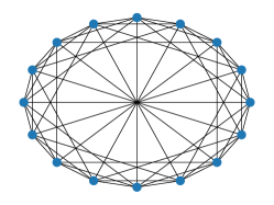
(a) Exponential network, $n=16$.

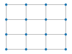
(b) Grid network, $n=16$.

Figure 1: Illustration of two network topologies.

5.1 Logistic Regression

We consider a binary classification problem using logistic regression (31). Each agent possesses a distinct local dataset $\mathcal{S}_{i}$ selected from the whole dataset $\mathcal{S}$. The classifier can then be obtained by solving the following convex optimization problem using all the agents’ local datasets $\mathcal{S}_{i},i=1,2,...,n$:

$$\min_{x\in\mathbb{R}^{785}}f(x)=\frac{1}{n}\sum_{i=1}^{n}f_{i}(x),$$ (31a)

$$f_{i}(x):=\frac{1}{|\mathcal{S}_{i}|}\sum_{j\in\mathcal{S}_{i}}\log\left[1+\exp(-x^{\intercal}u_{j}v_{j})\right]+\frac{\rho}{2}\left\|x\right\|^{2}.$$ (31b)

For Problem (31), we first consider the MNIST dataset [16]. We set $\rho=1/5$ and use decreasing stepsize $5/(k+100)$ for all the algorithms. The parameters of Algorithm 1 are chosen as $\alpha=0.1$ and $\gamma=0.004$. As shown in Table 1, it is sufficient to compare CEDAS with Choco-SGD, which previously enjoys the shortest transient time. The parameter of Choco-SGD is also set as $\gamma=0.004$. The performance of those uncompressed decentralized methods is presented as the baseline.

We first illustrate the performance of different algorithms via the residual error $\sum_{i=1}^{n}\mathbb{E}\left[\left\|x_{i,k}-x^{*}\right\|^{2}\right]/n$ against the number of iterations in Figure 2. It can be seen that, regarding the asymptotic network independent property of CEDAS, the results are consistent with our theoretical finding, that is, it takes more iterations for CEDAS to achieve comparable performance with centralized SGD when the connectivity of the network becomes worse (from an exponential network to a grid network). Moreover, the performance of CEDAS is better than that of Choco-SGD for both graphs (under different compressors). The superiority of CEDAS is more evident in a grid network.

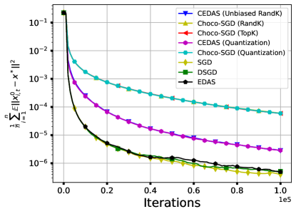
(a) Grid network, $n=100$, $1-\lambda_{2}=0.013$

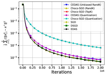
(b) Exponential network, $n=100$, $1-\lambda_{2}=0.133$.

Figure 2: Residual against the number of iterations. The results are averaged over $10$ repeated runs.

Then we check the variation of the residual error while fixing the total transmitted bits of each node in Figure 3. As shown in Figure 3, the compressed decentralized methods achieve better accuracy compared to their uncompressed counterparts under the same trasmitted bits. In particular, CEDAS achieves better performance compared to Choco-SGD. Such a difference becomes more evident when the graph connectivity is worse (in a grid network).

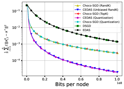
(a) Grid network, $n=100$, $1-\lambda_{2}=0.013$

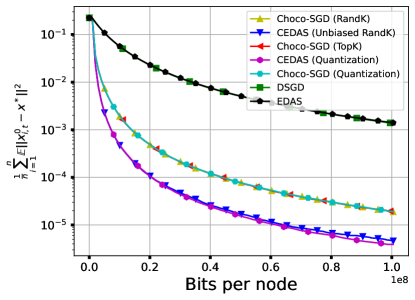
(b) Exponential network, $n=100$, $1-\lambda_{2}=0.133$.

Figure 3: Residual against the communicated bits. The results are averaged over $5$ repeated runs.

5.2 Neural Network

For the nonconvex case, we consider training a neural network with one hidden layer of $64$ neurons for a $10$-class classification problem on the MNIST dataset. We use constant stepsize $\eta=0.1$ and set the parameter $\alpha=0.1$ and $\gamma=0.004$. The dimension of the problem is $p=51675$. Figure 4 illustrates the performance of Choco-SGD and CEDAS with different compressors and their uncompressed counterparts DSGD and EDAS. When fixing the total transmitted bits, the compressed decentralized methods are preferable compared to their uncompressed counterparts. Particularly, the proposed CEDAS algorithm enjoys the best performance as illustrated in Figure 4.

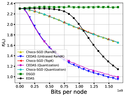
(a) Grid network, $n=25$, $1-\lambda_{2}=0.054$

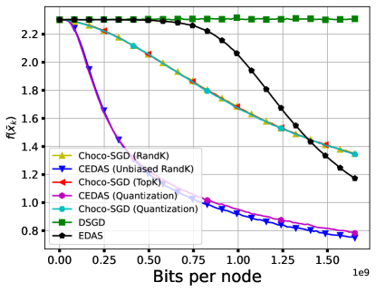
(b) Exponential network, $n=25$, $1-\lambda_{2}=0.305$.

Figure 4: Loss against communicated bits. The results are averaged over $2$ repeated runs.

Appendix A LEAD Algorithm

Algorithm 2 LEAD in Agent’s Perspective

1:Stepsize $\eta$, parameters $\gamma$ and $\alpha$, and initial values $x_{i,-1},h_{i,0},z_{i},i\in[n]$.

2:for Agent $i$ in parallel do

3:     $a_{i,0}=z_{i}-\sum_{j\in\mathcal{N}_{i}\cup\left\{i\right\}}w_{ij}z_{j}$

4:     $(h_{w})_{i,0}=\sum_{j\in\mathcal{N}_{i}\cup\left\{i\right\}}w_{ij}h_{j,0}$

5:     Compute $\nabla f_{i}(x_{i,-1};\xi_{i,-1})$ and $x_{i,0}=x_{i,-1}-\eta\nabla f_{i}(x_{i,-1};\xi_{i,-1})$

6:end for

7:for $k=0,1,\cdots,K-1$, agent $i$ in parallel do

8:     Compute $\nabla f_{i}(x_{i,k};\xi_{i,k})$

9:     $y_{i,k}=x_{i,k}-\eta\nabla f_{i}(\mathbf{x}_{i,k};\xi_{i,k})-\eta a_{i,k}$

10:     $\hat{y}_{i,k},(\hat{y}_{w})_{i,k},h_{i,k+1},(h_{w})_{i,k+1}$ = COMM($y_{i,k},h_{i,k},(h_{w})_{i,k},\alpha$)

11:     $a_{i,k+1}=a_{i,k}+\frac{\gamma}{2\eta}\left(\hat{y}_{i,k}-(\hat{y}_{w})_{i,k}\right)$

12:     $x_{i,k+1}=x_{i,k}-\eta\nabla f_{i}(x_{i,k};\xi_{i,k})-\eta a_{i,k+1}$

13:end for

14:Output $x_{i,K}$.

Appendix B Transformed Error Dynamics

As discussed in the subsection 2.2, Algorithm 1 can take a form similar to EDAS [8]. In this subsection, we state some results adapted from [8]. In particular, Lemmas B.1-B.3 and 3.1 are similar to those in [8] with a new mixing matrix $\tilde{W}=I-\gamma(I-W)/2$. Here, we can regard $\gamma$ as the parameter that controls the consensus update. Lemma B.4 utilizes the structure of $U_{L}$ and $U_{R}$ introduced in Lemma B.3 to simplify the presentation.

In light of Lemma 2.3 and the strong convexity of $f$, we can establish the error dynamics for (14) by choosing the unique pair of $(\mathbf{x}^{*},\mathbf{s}^{*}_{k})$ stated in Lemma B.1 below. The proof can be seen in [8, Lemma 2].

Lemma B.1.

Let Assumptions 2.1 and 2.5 hold, there exists $(\mathbf{x}^{*},\mathbf{s}_{k}^{*})$ that satisfies (15a). In particular, we can choose

$$\mathbf{x}^{*}=\mathbf{1}(x^{*})^{\intercal},$$ (32a)

$$\mathbf{s}_{k}^{*}=-\tilde{V}^{-}(\eta_{k}\nabla F(\mathbf{x}^{*})),$$ (32b)

where $x^{*}\in\mathbb{R}^{p}$ is the unique solution to Problem (1), $\tilde{V}^{-}$ is the pseudoinverse of $\tilde{V}$ given by $\tilde{V}^{-}=Q\left(\sqrt{I_{n}-\tilde{\Lambda}}\right)^{-}Q^{\intercal}$, and $Q$ is the same orthogonal matrix as in decomposing $W$, i.e., $W=Q\Lambda Q^{\intercal}$ with $\Lambda=\mathrm{diag}(\lambda_{1},\lambda_{2},\cdots,\lambda_{n})$. $\left(\sqrt{I_{n}-\tilde{\Lambda}}\right)^{-}:=\mathrm{\mathrm{diag}}(p_{1},p_{2},...,p_{n})$ is the pseudoinverse of $\sqrt{I_{n}-\tilde{\Lambda}}$ with

$$p_{i}=\begin{cases}\frac{1}{\sqrt{1-\tilde{\lambda}_{i}}}&\text{if }1-\tilde{\lambda}_{i}\neq 0,\\ 0&\text{otherwise.}\end{cases}$$

In light of Lemma B.1, the dynamics of (14) can be written in a matrix form stated in Lemma B.2.

Lemma B.2.

Let Assumptions 2.1 and 2.5 hold and denote $\hat{\mathbf{x}}_{k}:=\mathbf{x}_{k}-\mathbf{x}^{*}$, $\hat{\mathbf{s}}_{k}:=\mathbf{s}_{k}-\mathbf{s}^{*}_{k}$, and $\hat{\mathbf{g}}_{k}:=\nabla F(\mathbf{x}_{k})-G_{k}$. We have

$$\begin{pmatrix}\hat{\mathbf{x}}_{k+1}\\ \hat{\mathbf{s}}_{k+1}\end{pmatrix} =B_{1}\begin{pmatrix}\hat{\mathbf{x}}_{k}+\eta_{k}\left(\nabla F(\mathbf{x}^{*})-\nabla F(\mathbf{x}_{k})\right)\\ \hat{\mathbf{s}}_{k}\end{pmatrix}+B_{2}\begin{pmatrix}\eta_{k}\hat{\mathbf{g}}_{k}\\ E_{k}\end{pmatrix}+\begin{pmatrix}\mathbf{0}\\ \mathbf{s}_{k}^{*}-\mathbf{s}_{k+1}^{*}\end{pmatrix},$$

where

$$B_{1}=\begin{pmatrix}\tilde{W}&-\tilde{W}\tilde{V}\\ \tilde{V}&\tilde{W}\end{pmatrix},\ B_{2}=\begin{pmatrix}\tilde{W}&-(I-\tilde{W})\\ \tilde{V}&\tilde{V}\end{pmatrix}.$$

Proof.

According to Lemma 2.3, we have $(\tilde{W}-I)\mathbf{s}^{*}_{k}=\eta_{k}\tilde{V}\nabla F(\mathbf{x}^{*})$, then

$$\hat{\mathbf{s}}_{k+1} =\mathbf{s}_{k+1}-\mathbf{s}^{*}_{k+1}$$

$$=\tilde{W}(\mathbf{s}_{k}-\mathbf{s}^{*}_{k})+\tilde{W}\mathbf{s}^{*}_{k}-\mathbf{s}^{*}_{k+1}+\tilde{V}\left(\mathbf{x}_{k}-\mathbf{x}^{*}-\eta_{k}G_{k}\right)+\tilde{V}E_{k}$$

$$=\tilde{W}\hat{\mathbf{s}}_{k}+\tilde{V}\left[\hat{\mathbf{x}}_{k}+\eta_{k}(\nabla F(\mathbf{x}^{*})-\nabla F(\mathbf{x}_{k}))\right]+\eta_{k}\tilde{V}\hat{\mathbf{g}}_{k}+\tilde{V}E_{k}+\mathbf{s}_{k}^{*}-\mathbf{s}_{k+1}^{*}.$$

Lemma 2.3 also implies $\tilde{W}\tilde{V}\mathbf{s}^{*}_{k}+\eta_{k}\tilde{W}\nabla F(\mathbf{x}^{*})=0$ and $\tilde{W}\mathbf{x}^{*}=\mathbf{x}^{*}$, then

$$\hat{\mathbf{x}}_{k+1} =\mathbf{x}_{k+1}-\mathbf{x}^{*}$$

$$=\tilde{W}\left(\mathbf{x}_{k}-\mathbf{x}^{*}-\eta_{k}G_{k}\right)-\tilde{W}\tilde{V}(\mathbf{s}_{k}-\mathbf{s}^{*}_{k})-\tilde{W}\tilde{V}\mathbf{s}^{*}_{k}-(I-\tilde{W})E_{k}$$

$$=\tilde{W}\left[\hat{\mathbf{x}}_{k}+\eta_{k}\left(\nabla F(\mathbf{x}^{*})-\nabla F(\mathbf{x}_{k})\right)\right]+\eta_{k}\tilde{W}\hat{\mathbf{g}}_{k}-\tilde{W}\tilde{V}\hat{\mathbf{s}}_{k}-(I-\tilde{W})E_{k}.$$

∎

Similar to the arguments in [8], we conclude in Lemma B.3 that $B_{1}$ has an eigendecomposition $B_{1}=UPU^{-1}$. This guides us to consider the transformed error dynamics in Lemma 3.1.

Lemma B.3.

Let Assumption 2.1 hold, the matrix $B_{1}\in\mathbb{R}^{2n\times 2n}$ has a decomposition given by

$$B_{1}=UPU^{-1}:=\begin{pmatrix}\mathbf{1}_{n}&\mathbf{0}&U_{R,u}\\ \mathbf{0}&\mathbf{1}_{n}&U_{R,l}\end{pmatrix}\mathrm{diag}(1,1,P_{1})\begin{pmatrix}\frac{1}{n}\mathbf{1}_{n}^{\intercal}&\mathbf{0}\\ \mathbf{0}&\frac{1}{n}\mathbf{1}_{n}^{\intercal}\\ U_{L,l}&U_{L,r}\end{pmatrix},$$

where $P_{1}$ is a diagonal matrix with complex entries, matrices $U_{R,u},U_{R,l}\in\mathbb{R}^{n\times 2(n-1)}$, and $U_{L,l},U_{L,r}\in\mathbb{R}^{2(n-1)\times n}$ are introduced to denote

$$U_{R}:=\begin{pmatrix}U_{R,u}\\ U_{R,l}\end{pmatrix},\quad U_{L}:=\begin{pmatrix}U_{L,l}&U_{L,r}\end{pmatrix},$$

then the product $\|U_{L}\|_{2}^{2}\|U_{R}\|_{2}^{2}$ has an upper bound that is independent of $n$. More specifically,

$$\|U_{L}\|_{2}^{2}\|U_{R}\|_{2}^{2}\leq\frac{1}{\tilde{\lambda}_{n}}\leq\frac{1}{1-\gamma},$$

where $\tilde{\lambda}_{n}=1-\gamma(1-\lambda_{n})/2>(1-\gamma)$.

Remark B.1.

According to Lemma 2.2, $\tilde{W}$ is positive definite. Hence, we no longer need to assume $W$ is positive definite as in [8].

Proof.

Since the matrix $W$ is symmetric, it has eigendecomposition $W=Q\Lambda Q^{\intercal}$, where $Q$ is an orthogonal matrix, and $\Lambda:=\mathrm{diag}\left(1,\lambda_{2},\ldots,\lambda_{n}\right).$ Then, $\tilde{W}=I-\frac{\gamma}{2}(I-W)$ and $\tilde{V}=(I-\tilde{W})^{1/2}$ have the following decomposition:

$$\tilde{W}=Q\tilde{\Lambda}Q^{\intercal},\tilde{V}=Q\sqrt{I-\tilde{\Lambda}}Q^{\intercal},$$ (33)

where $\tilde{\Lambda}=\mathrm{diag}\left(1,1-\gamma(1-\lambda_{2})/2,\cdots,1-\gamma(1-\lambda_{n})/2\right)\succ 0$ given $\gamma\in(0,1)$. Therefore,

$$B_{1} =\begin{pmatrix}Q&\\ &Q\end{pmatrix}\begin{pmatrix}\tilde{\Lambda}&-\tilde{\Lambda}\sqrt{I-\tilde{\Lambda}}\\ \sqrt{I-\tilde{\Lambda}}&\tilde{\Lambda}\end{pmatrix}\begin{pmatrix}Q^{\intercal}&\\ &Q^{\intercal}\end{pmatrix}.$$ (34)

Noticing the particular form of the middle term on the right-hand side of (34), there exists a permutation operator $\Pi_{1}\in\mathbb{R}^{2n\times 2n}$ such that

$$\begin{pmatrix}\tilde{\Lambda}&-\tilde{\Lambda}\sqrt{I-\tilde{\Lambda}}\\ \sqrt{I-\tilde{\Lambda}}&\tilde{\Lambda}\end{pmatrix}=\Pi_{1}\mathrm{diag}(\Gamma_{1},\Gamma_{2},...,\Gamma_{n})\Pi_{1}^{\intercal},$$ (35)

where

$$\Gamma_{1}:=I_{2},\;\Gamma_{t}:=\begin{pmatrix}\tilde{\lambda}_{t}&-\tilde{\lambda}_{t}\sqrt{1-\tilde{\lambda}_{t}}\\ \sqrt{1-\tilde{\lambda}_{t}}&\tilde{\lambda}_{t}\end{pmatrix},t=2,\ldots,n.$$ (36)

Hence,

$$B_{1}=\begin{aligned} \left(\begin{array}[]{cc}Q&\\ &Q\end{array}\right)\Pi_{1}\mathrm{diag}(I_{2},\Gamma_{2},...,\Gamma_{n})\Pi_{1}^{\intercal}\left(\begin{array}[]{cc}Q^{\intercal}&\\ &Q^{\intercal}\end{array}\right).\end{aligned}$$ (37)

We then consider the eigendecomposition of $\Gamma_{t}$ for $t=2,3,\ldots,n$. It can be verified that

$$\Gamma_{t}=Z_{t}\left(\begin{array}[]{cc}\tilde{\lambda}_{t}+i\sqrt{\tilde{\lambda}_{t}-\tilde{\lambda}_{t}^{2}}&0\\ 0&\tilde{\lambda}_{t}-i\sqrt{\tilde{\lambda}_{t}-\tilde{\lambda}_{t}^{2}}\end{array}\right)Z_{t}^{-1},$$ (38)

where $i^{2}=-1$, and

$$Z_{t}=\begin{pmatrix}i\sqrt{\tilde{\lambda}_{t}}&-i\sqrt{\tilde{\lambda}_{t}}\\ 1&1\end{pmatrix},\quad Z_{t}^{-1}=\frac{1}{2i\sqrt{\tilde{\lambda}_{t}}}\begin{pmatrix}1&i\sqrt{\tilde{\lambda}_{t}}\\ -1&i\sqrt{\tilde{\lambda}_{t}}\end{pmatrix},t\geq 2$$ (39)

Therefore, from (37),

$$B_{1}=\begin{pmatrix}Q&\\ &Q\end{pmatrix}\Pi_{1}Z\left(\mathrm{diag}(I_{2},P_{1})\right)Z^{-1}\Pi_{1}^{\intercal}\begin{pmatrix}Q^{\intercal}&\\ &Q^{\intercal}\end{pmatrix},$$

where $Z=\mathrm{diag}\left(I_{2},Z_{2},Z_{3},...,Z_{n}\right)$ and $P_{1}$ is a complex diagonal matrix.

Additionally, note that $\left(\mathbf{1}_{n}^{\intercal},\mathbf{0}^{\intercal}\right)^{\intercal}$ and $\left(\mathbf{0}^{\intercal},\mathbf{1}_{n}^{\intercal}\right)^{\intercal}$ are the two eigenvectors of $B_{1}$ w.r.t. eigenvalue $1$. Thus, after a permutation $\Pi_{2}$, we reach a decomposition for $B_{1}$ given by $B_{1}=UPU^{-1}$, where

$$P:=\mathrm{diag}(I_{2},P_{1}),$$

$$U:=\begin{pmatrix}Q&\\ &Q\end{pmatrix}\Pi_{1}Z\Pi_{2}=\begin{pmatrix}\mathbf{1}_{n}&\mathbf{0}&U_{R,u}\\ \mathbf{0}&\mathbf{1}_{n}&U_{R,l}\end{pmatrix},$$

for some $U_{R,u},U_{R,l}\in\mathbb{R}^{n\times(2n-2)}$. We next bound $\|U_{R}\|_{2}$ and $\|U_{L}\|_{2}$. By definition, we have

$$\|U_{R}\|_{2}\leq\|U\|_{2} \leq\left\|\begin{pmatrix}Q&\\ &Q\end{pmatrix}\right\|_{2}\|\Pi_{1}\|_{2}\|Z\|_{2}\|\Pi_{2}\|_{2}=\|Z\|_{2}.$$

Since $\forall t=2,3,\ldots,n,$

$$\|Z_{t}\|_{2} =\sqrt{\lambda_{\max}(Z_{t}Z_{t}^{*})}=\sqrt{\lambda_{\max}\left(\begin{array}[]{cc}2\tilde{\lambda}_{t}&0\\ 0&2\end{array}\right)}=\sqrt{2},\;$$

we obtain $\|U_{R}\|_{2}\leq\|Z\|_{2}=\sqrt{2}$. Similarly, $\|U_{L}\|_{2}\leq\|\tilde{U}^{-1}\|_{2}\leq\|Z^{-1}\|_{2}.$

Given that

$$Z_{t}^{-1}(Z_{t}^{-1})^{*}=\frac{1}{4}\begin{pmatrix}1+\frac{1}{\tilde{\lambda}_{t}}&1-\frac{1}{\tilde{\lambda}_{t}}\\ 1-\frac{1}{\tilde{\lambda}_{t}}&1+\frac{1}{\tilde{\lambda}_{t}},\end{pmatrix}$$

we have $\|Z_{t}^{-1}\|_{2}=\sqrt{\lambda_{\max}(Z_{t}^{-1}(Z_{t}^{-1})^{*})}=\sqrt{\frac{1}{2\tilde{\lambda}_{t}}}.$ Hence, $\|U_{L}\|_{2}\leq\|Z^{-1}\|_{2}=\sqrt{\frac{1}{2\tilde{\lambda}_{n}}}$. ∎

Lemma B.4 reveals some properties of the block matrices introduced in Lemma B.3. It helps us simplify the transformed error dynamics in Lemma 3.1.

Lemma B.4.

Let Assumption 2.1 hold, we have

$$U_{R,l}U_{L,l}=U_{R,u}U_{L,r}=\mathbf{0},\ U_{L,l}U_{R,u}+U_{L,r}U_{R,l}=I_{2n-2}$$

$$\frac{\mathbf{1}\mathbf{1}^{\intercal}}{n}+U_{R,u}U_{L,l}=\frac{\mathbf{1}\mathbf{1}^{\intercal}}{n}+U_{R,l}U_{L,r}=I_{n},$$

$$U_{L,l}\tilde{W}+U_{L,r}\tilde{V}=P_{1}U_{L,l},\ U_{L,r}\tilde{W}-U_{L,l}\tilde{W}\tilde{V}=P_{1}U_{L,r}$$

$$\tilde{W}U_{R,u}-\tilde{W}\tilde{V}U_{R,l}=U_{R,u}P_{1},\ \tilde{V}U_{R,u}+\tilde{W}U_{R,l}=U_{R,l}P_{1}$$

Proof.

From $UU^{-1}=I_{2n}$ and $U^{-1}U=I_{2n}$, we have

$$UU^{-1}=\begin{pmatrix}\mathbf{1}_{n}&\mathbf{0}&U_{R,u}\\ \mathbf{0}&\mathbf{1}_{n}&U_{R,l}\end{pmatrix}\begin{pmatrix}\frac{1}{n}\mathbf{1}_{n}^{\intercal}&\mathbf{0}\\ \mathbf{0}&\frac{1}{n}\mathbf{1}_{n}^{\intercal}\\ U_{L,l}&U_{L,r}\end{pmatrix}=\begin{pmatrix}\frac{\mathbf{1}\mathbf{1}^{\intercal}}{n}+U_{R,u}U_{L,l}&U_{R,u}U_{L,r}\\ U_{R,l}U_{L,l}&\frac{\mathbf{1}\mathbf{1}^{\intercal}}{n}+U_{R,l}U_{L,r}\end{pmatrix}=\begin{pmatrix}I_{n}&\mathbf{0}\\ \mathbf{0}&I_{n}\end{pmatrix},$$

$$U^{-1}U=\begin{pmatrix}\frac{1}{n}\mathbf{1}_{n}^{\intercal}&\mathbf{0}\\ \mathbf{0}&\frac{1}{n}\mathbf{1}_{n}^{\intercal}\\ U_{L,l}&U_{L,r}\end{pmatrix}\begin{pmatrix}\mathbf{1}_{n}&\mathbf{0}&U_{R,u}\\ \mathbf{0}&\mathbf{1}_{n}&U_{R,l}\end{pmatrix}=\begin{pmatrix}1&\mathbf{0}&\frac{1}{n}\mathbf{1}^{\intercal}_{n}U_{R,u}\\ \mathbf{0}&1&\frac{1}{n}\mathbf{1}^{\intercal}_{n}U_{R,l}\\ U_{L,l}\mathbf{1}_{n}&U_{L,r}\mathbf{1}_{n}&U_{L,l}U_{R,u}+U_{L,r}U_{R,l}\end{pmatrix}=\begin{pmatrix}1&\mathbf{0}&\mathbf{0}\\ \mathbf{0}&1&\mathbf{0}\\ \mathbf{0}&\mathbf{0}&I_{2n-2}\end{pmatrix}$$

According to $PU^{-1}=U^{-1}B_{1}$, we obtain

$$U^{-1}B_{1}=\begin{pmatrix}\frac{1}{n}\mathbf{1}_{n}^{\intercal}&\mathbf{0}\\ \mathbf{0}&\frac{1}{n}\mathbf{1}_{n}^{\intercal}\\ U_{L,l}&U_{L,r}\end{pmatrix}\begin{pmatrix}\tilde{W}&-\tilde{W}\tilde{V}\\ \tilde{V}&\tilde{W}\end{pmatrix}=\begin{pmatrix}\frac{1}{n}\mathbf{1}^{\intercal}_{n}&\mathbf{0}\\ \mathbf{0}&\frac{1}{n}\mathbf{1}^{\intercal}_{n}\\ U_{L,l}\tilde{W}+U_{L,r}\tilde{V}&U_{L,r}\tilde{W}-U_{L,l}\tilde{W}\tilde{V}\end{pmatrix}=\begin{pmatrix}\frac{1}{n}\mathbf{1}^{\intercal}_{n}&\mathbf{0}\\ \mathbf{0}&\frac{1}{n}\mathbf{1}^{\intercal}_{n}\\ P_{1}U_{L,l}&P_{1}U_{L,r}\end{pmatrix}.$$

From $UP=B_{1}U$, we have

$$B_{1}U =\begin{pmatrix}\tilde{W}&-\tilde{W}\tilde{V}\\ \tilde{V}&\tilde{W}\end{pmatrix}\begin{pmatrix}\mathbf{1}_{n}&\mathbf{0}&U_{R,u}\\ \mathbf{0}&\mathbf{1}_{n}&U_{R,l}\end{pmatrix}=\begin{pmatrix}\mathbf{1}_{n}&\mathbf{0}&\tilde{W}U_{R,u}-\tilde{W}\tilde{V}U_{R,l}\\ \mathbf{0}&\mathbf{1}_{n}&\tilde{V}U_{R,u}+\tilde{W}U_{R,l}\end{pmatrix}=\begin{pmatrix}\mathbf{1}_{n}&\mathbf{0}&U_{R,u}P_{1}\\ \mathbf{0}&\mathbf{1}_{n}&U_{R,l}P_{1}\end{pmatrix}.$$

The above implies the desired results. ∎

Appendix C Proofs for strongly convex case

C.1 Proof of Lemma 2.1

Proof.

We first show the operator $\mathcal{C}$ is unbiased. Since $\mathcal{C}_{2}\in\mathbb{U}(C_{2})$, we have

$$\mathbb{E}\left[\mathcal{C}(x)\middle|x\right] =\mathbb{E}\left[\mathcal{C}_{1}(x)+\mathcal{C}_{2}\left(x-\mathcal{C}_{1}(x)\right)\middle|x\right]$$

$$=\mathbb{E}\left[\mathbb{E}\left[\mathcal{C}_{1}(x)+\mathcal{C}_{2}\left(x-\mathcal{C}_{1}(x)\right)\middle|\mathcal{C}_{1}(x)\right]\middle|x\right]$$

$$=\mathbb{E}\left[\mathcal{C}_{1}(x)+x-\mathcal{C}_{1}(x)\middle|x\right]$$

$$=x.$$

The remaining condition can be verified by

$$\mathbb{E}\left[\left\|\mathcal{C}(x)-x\right\|^{2}\middle|x\right] =\mathbb{E}\left[\left\|\mathcal{C}_{1}(x)+\mathcal{C}_{2}\left(x-\mathcal{C}_{1}(x)\right)-x\right\|^{2}\middle|x\right]$$

$$=\mathbb{E}\left[\mathbb{E}\left[\left\|\mathcal{C}_{1}(x)+\mathcal{C}_{2}\left(x-\mathcal{C}_{1}(x)\right)-x\right\|^{2}\middle|\mathcal{C}_{1}(x)\right]\middle|x\right]$$

$$\leq\mathbb{E}\left[\left\|\mathcal{C}_{1}(x)-x\right\|^{2}\middle|x\right]+(C_{2}+1)\mathbb{E}\left[\left\|x-\mathcal{C}_{1}(x)\right\|^{2}\middle|x\right]-2\mathbb{E}\left[\left\|\mathcal{C}_{1}(x)-x\right\|^{2}\middle|x\right]$$

$$\leq C_{2}(1-\delta_{1})\left\|x\right\|^{2}.$$

∎

C.2 Proof of Lemma 2.3

Proof.

From Lemma 2.2, $\tilde{W}$ is doubly stochastic and $\mathrm{Null}(\tilde{V})=\left\{\mathbf{1}\right\}$, then (15a) implies $\mathbf{x}^{*}\in\mathrm{Null}(\tilde{V})$. Hence, $x_{1}^{*}=x_{2}^{*}=\cdots=x^{*}_{n}$. Multiplying $\mathbf{1}^{\intercal}$ to (15b) gives $\eta_{k}\sum_{i=1}^{n}\nabla f_{i}(x_{i}^{*})=0$, which indicates that $x_{i}^{*},i=1,2,\cdots,n$ must coincide with $x^{*}$. In summary, we have $x_{1}^{*}=x_{2}^{*}=\cdots=x^{*}_{n}=x^{*}$. ∎

C.3 Proof of Lemma 3.1

Proof.

Note that $\mathbf{s}_{k}\in\mathrm{Span}\left(I-W\right)$, we then have

$$U^{-1}\begin{pmatrix}\hat{\mathbf{x}}_{k}\\ \hat{\mathbf{s}}_{k}\end{pmatrix}=\begin{pmatrix}\frac{\mathbf{1}^{\intercal}}{n}\hat{\mathbf{x}}_{k}\\ \frac{\mathbf{1}^{\intercal}}{n}\mathbf{s}_{k}\\ U_{L,l}\hat{\mathbf{x}}_{k}+U_{L,r}\hat{\mathbf{s}}_{k}\end{pmatrix}.$$ (40)

Multiplying $U^{-1}$ to the recursion in Lemma B.2 yields

$$\begin{pmatrix}\bar{z}_{k+1}^{\intercal}\\ \frac{\mathbf{1}^{\intercal}}{n}\hat{\mathbf{s}}_{k+1}\\ \check{z}_{k+1}\end{pmatrix} =\begin{pmatrix}\bar{z}_{k}^{\intercal}+\frac{\eta_{k}}{n}\mathbf{1}^{\intercal}\left(\nabla F(\mathbf{x}^{*})-\nabla F(\mathbf{x}^{k})\right)\\ \frac{\mathbf{1}^{\intercal}}{n}\hat{\mathbf{s}}_{k}\\ P_{1}\check{z}_{k}+\eta_{k}P_{1}U_{L,l}\left(\nabla F(\mathbf{x}^{*})-\nabla F(\mathbf{x}^{k})\right)\end{pmatrix}$$

$$\quad+\begin{pmatrix}\frac{\eta_{k}}{n}\mathbf{1}^{\intercal}\hat{\mathbf{g}}_{k}\\ 0\\ \eta_{k}\left(U_{L,l}\tilde{W}+U_{L,r}\tilde{V}\right)\hat{\mathbf{g}}_{k}+\left[U_{L,r}\tilde{V}-U_{L,l}(I-\tilde{W})\right]E_{k}\end{pmatrix}$$

$$\quad+\begin{pmatrix}0\\ \frac{\mathbf{1}^{\intercal}}{n}(\mathbf{s}_{k}^{*}-\mathbf{s}_{k+1}^{*})\\ U_{L,r}\left(\mathbf{s}_{k}^{*}-\mathbf{s}_{k+1}^{*}\right)\end{pmatrix}$$

Invoking the following results from Lemma B.4, we obtain the desired recursion for $\left\{\check{z}_{k}\right\}$.

$$U_{L,r}\tilde{V}-U_{L,l}(I-\tilde{W}) =P_{1}U_{L,l}-U_{L,l},$$

$$U_{L,l}\tilde{W}+U_{L,r}\tilde{V} =P_{1}U_{L,l}.$$

∎

C.4 Proof of Lemma 3.2

Proof.

In the following proofs, we use two sets of filtration $\mathcal{G}_{k}$ and $\mathcal{F}_{k}$ similar to those defined in [22]. We denote $\left\{\mathcal{G}_{k}\right\}_{k\geq 0}$ as the $\sigma-$algebra generated by gradient sampling and define $\left\{\mathcal{F}_{k}\right\}_{k\geq 0}$ as the $\sigma-$algebra generated by the compression. Then,

$$\mathcal{G}_{0}\subset\mathcal{F}_{0}\subset\mathcal{G}_{1}\subset\mathcal{F}_{1}\subset\mathcal{G}_{2}\subset\mathcal{F}_{2}\subset\cdots\subset\mathcal{G}_{k}\subset\mathcal{F}_{k}\subset\cdots$$

We start by stating the relation between $\left\{\hat{\mathbf{x}}_{k},\hat{\mathbf{s}}_{k}\right\}$ and $\left\{\bar{z}_{k},\check{z}_{k}\right\}$ according to (40):

$$\hat{\mathbf{x}}_{k}=\mathbf{1}\bar{z}_{k}^{\intercal}+U_{R,u}\check{z}_{k},\ \tilde{V}\hat{\mathbf{s}}_{k}=\tilde{V}U_{R,l}\check{z}_{k}.$$ (41)

Consider the recursion of $\check{z}_{k}$ in Lemma 3.1, taking conditioned expectation with respect to $\mathcal{F}_{k}$ and using Assumption 2.3 lead to

$$\mathbb{E}\left[\left\|\check{z}_{k+1}\right\|^{2}\middle|\mathcal{F}_{k}\right]\leq\left\|\mathcal{A}_{1}\right\|^{2}+C\left\|(P_{1}-I)U_{L,l}\right\|^{2}\left\|\mathbf{y}_{k}-H_{k}\right\|^{2},$$ (42)

where

$$\mathcal{A}_{1} :=P_{1}\check{z}_{k}+\eta_{k}P_{1}U_{L,l}\left(\nabla F(\mathbf{x}^{*})-\nabla F(\mathbf{x}^{k})\right)+\eta_{k}P_{1}U_{L,l}\hat{\mathbf{g}}_{k}+U_{L,r}\left(\mathbf{s}_{k}^{*}-\mathbf{s}_{k+1}^{*}\right).$$

We next consider $\left\|\mathcal{A}_{1}\right\|^{2}$ with Assumption 2.2,

$$\mathbb{E}\left[\left\|\mathcal{A}_{1}\right\|^{2}\middle|\mathcal{G}_{k}\right]=\left\|P_{1}\check{z}_{k}+\eta_{k}P_{1}U_{L,l}\left(\nabla F(\mathbf{x}^{*})-\nabla F(\mathbf{x}^{k})\right)+U_{L,r}\left(\mathbf{s}_{k}^{*}-\mathbf{s}_{k+1}^{*}\right)\right\|^{2}+\eta_{k}^{2}\mathbb{E}\left[\left\|P_{1}U_{L,l}\hat{\mathbf{g}}_{k}\right\|^{2}\middle|\mathcal{G}_{k}\right]$$ (43)

$$\leq(1+q)\left\|P_{1}\check{z}_{k}\right\|^{2}+(1+q^{-1})\left\|\eta_{k}P_{1}U_{L,l}\left(\nabla F(\mathbf{x}^{*})-\nabla F(\mathbf{x}^{k})\right)+U_{L,r}\left(\mathbf{s}_{k}^{*}-\mathbf{s}_{k+1}^{*}\right)\right\|^{2}+\eta_{k}^{2}\tilde{\lambda}_{2}\left\|U_{L}\right\|^{2}n\sigma^{2}$$

$$\leq\frac{1+\tilde{\lambda}_{2}}{2}\left\|\check{z}_{k}\right\|^{2}+\frac{4\eta_{k}^{2}\tilde{\lambda}_{2}\left\|U_{L}\right\|^{2}}{1-\tilde{\lambda}_{2}}\left\|\nabla F(\mathbf{x}^{*})-\nabla F(\mathbf{x}^{k})\right\|^{2}+\frac{4\tilde{\lambda}_{2}\left\|U_{L}\right\|^{2}}{1-\tilde{\lambda}_{2}}\left\|\mathbf{s}_{k}^{*}-\mathbf{s}_{k+1}^{*}\right\|^{2}+\eta_{k}^{2}\tilde{\lambda}_{2}\left\|U_{L}\right\|^{2}n\sigma^{2},$$

where we apply Young’s inequality for $q=(1-\tilde{\lambda}_{2})/(2\tilde{\lambda}_{2})$ and invoke $\left\|P_{1}\right\|=\sqrt{\tilde{\lambda}_{2}}$ according to the proof of Lemma B.3. In addition, we have from Assumptions 2.5 and (41) that

$$\left\|\nabla F(\mathbf{x}^{*})-\nabla F(\mathbf{x}_{k})\right\|^{2} \leq L^{2}\left\|\mathbf{x}_{k}-\mathbf{x}^{*}\right\|^{2}$$ (44)

$$=L^{2}\left(\left\|\mathbf{x}_{k}-\mathbf{1}\bar{x}_{k}^{\intercal}\right\|^{2}+n\left\|\bar{x}_{k}-x^{*}\right\|^{2}\right)$$

$$\leq nL^{2}\left\|\bar{z}_{k}\right\|^{2}+\left\|U_{R}\right\|^{2}L^{2}\left\|\check{z}_{k}\right\|^{2}.$$

In light of Lemma B.1, we have

$$\left\|\mathbf{s}_{k}^{*}-\mathbf{s}_{k+1}^{*}\right\|^{2}\leq\left\|\tilde{V}^{-}\right\|^{2}\left\|\nabla F(\mathbf{x}^{*})\right\|^{2}\left(\eta_{k}-\eta_{k+1}\right)^{2}.$$ (45)

Hence, taking conditioned expectation with respect to $\mathcal{G}_{k}\subset\mathcal{F}_{k}$ on both sides of (42), invoking tower property, and combining (43)-(45) yield

$$\mathbb{E}\left[\left\|\check{z}_{k+1}\right\|^{2}\middle|\mathcal{G}_{k}\right]\leq\left(\frac{1+\tilde{\lambda}_{2}}{2}+\frac{4\eta_{k}^{2}\tilde{\lambda}_{2}L^{2}\left\|U_{L}\right\|^{2}\left\|U_{R}\right\|^{2}}{1-\tilde{\lambda}_{2}}\right)\left\|\check{z}_{k}\right\|^{2}+\frac{4\eta_{k}^{2}\tilde{\lambda}_{2}L^{2}n\left\|U_{L}\right\|^{2}}{1-\tilde{\lambda}_{2}}\left\|\bar{z}_{k}\right\|^{2}+\eta_{k}^{2}\tilde{\lambda}_{2}\left\|U_{L}\right\|^{2}n\sigma^{2}$$ (46)

$$\quad+\left\|P_{1}-I\right\|^{2}\left\|U_{L}\right\|^{2}C\mathbb{E}\left[\left\|\mathbf{y}_{k}-H_{k}\right\|^{2}\middle|\mathcal{G}_{k}\right]+\frac{4\tilde{\lambda}_{2}\left\|U_{L}\right\|^{2}\left\|\tilde{V}^{-}\right\|^{2}\left\|\nabla F(\mathbf{x}^{*})\right\|^{2}}{1-\tilde{\lambda}_{2}}\left(\eta_{k}-\eta_{k+1}\right)^{2}$$

$$\leq\frac{3+\tilde{\lambda}_{2}}{4}\left\|\check{z}_{k}\right\|^{2}+\frac{4\eta_{k}^{2}L^{2}n}{1-\tilde{\lambda}_{2}}\left\|\bar{z}_{k}\right\|^{2}+\eta_{k}^{2}n\sigma^{2}+\gamma C\mathbb{E}\left[\left\|\mathbf{y}_{k}-H_{k}\right\|^{2}\middle|\mathcal{G}_{k}\right]+\frac{4\left\|\nabla F(\mathbf{x}^{*})\right\|^{2}}{(1-\tilde{\lambda}_{2})^{2}}\left(\eta_{k}-\eta_{k+1}\right)^{2},$$

where the last inequality holds by letting $\eta_{k}\leq\gamma(1-\lambda_{2})/(8\sqrt{2}L)$. Note from Lemmas B.1 and B.3 and given $\gamma\leq 1/2$, we have

$$\left\|P_{1}-I\right\|^{2}=\frac{\gamma}{2}(1-\lambda_{n})<\gamma,\ \left\|U_{L}\right\|^{2}\left\|U_{R}\right\|^{2}\leq\frac{1}{1-\gamma}\leq 2,\ \left\|U_{L}\right\|^{2}\leq\frac{1}{2\tilde{\lambda}_{n}}\leq 1,\ \left\|\tilde{V}^{-}\right\|^{2}=\frac{1}{1-\tilde{\lambda}_{2}}.$$

Taking full expectation on (46) yields the desired result.

∎

C.5 Proof of Lemma 3.3

Proof.

From Lemma 2.3, (8), and (41), we have

$$\left(I-\tilde{W}\right)\mathbf{y}_{k} =\left(I-\tilde{W}\right)\left(\mathbf{y}_{k}-\mathbf{x}^{*}\right)$$ (47)

$$=\left(I-\tilde{W}\right)\left[\mathbf{x}_{k}-\eta_{k}G_{k}-\tilde{V}\left(\mathbf{s}_{k}-\mathbf{s}_{k}^{*}\right)-\tilde{V}\mathbf{s}_{k}^{*}-\mathbf{x}^{*}\right]$$

$$=\left(I-\tilde{W}\right)\left[\hat{\mathbf{x}}_{k}-\tilde{V}\hat{\mathbf{s}}_{k}-\eta_{k}G_{k}+\eta_{k}\nabla F(\mathbf{x}^{*})\right]$$

$$=\left(I-\tilde{W}\right)\left[\mathbf{1}\bar{z}_{k}^{\intercal}+\left(U_{R,u}-\tilde{V}U_{R,l}\right)\check{z}_{k}+\eta_{k}\hat{\mathbf{g}}_{k}+\eta_{k}\left(\nabla F(\mathbf{x}^{*})-\nabla F(\mathbf{x}_{k})\right)\right]$$

$$=\tilde{V}U_{R,l}\left(P_{1}-I\right)\check{z}_{k}+\left(I-\tilde{W}\right)\eta_{k}\left[\hat{\mathbf{g}}_{k}+\left(\nabla F(\mathbf{x}^{*})-\nabla F(\mathbf{x}_{k})\right)\right],$$

where we invoke Lemma B.4 in the last inequality

$$\left(I-\tilde{W}\right)\left(U_{R,u}-\tilde{V}U_{R,l}\right) =\tilde{V}(\tilde{V}U_{R,u}-(I-\tilde{W})U_{R,l})=\tilde{V}U_{R,l}\left(P_{1}-I\right).$$

We next show the recursion for $\mathbb{E}\left[\left\|\mathbf{y}_{k}-H_{k}\right\|^{2}\right]$. In light of $\tilde{V}\mathbf{s}_{k}^{*}=-\eta_{k}\nabla F(\mathbf{x}^{*})$ and (47), we have

$$\mathbf{y}_{k+1}-H_{k+1}=\mathbf{x}_{k+1}-\eta_{k+1}G_{k+1}-{D}_{k+1}-H_{k}-\alpha\mathcal{C}\left(\mathbf{y}_{k}-H_{k}\right)$$ (48)

$$=\mathbf{x}_{k}-\eta_{k}G_{k}-{D}_{k+1}-\eta_{k+1}G_{k+1}-{D}_{k+1}-H_{k}-\alpha\mathcal{C}\left(\mathbf{y}_{k}-H_{k}\right)$$

$$=\mathbf{y}_{k}-H_{k}+{D}_{k}-2{D}_{k+1}-\eta_{k+1}G_{k+1}-\alpha E_{k}-\alpha(\mathbf{y}_{k}-H_{k})$$

$$=(1-\alpha)(\mathbf{y}_{k}-H_{k})-\alpha E_{k}-2\left(I-\tilde{W}\right)E_{k}-2\left(I-\tilde{W}\right)\mathbf{y}_{k}-\tilde{V}\hat{\mathbf{s}}_{k}+\eta_{k}\nabla F(\mathbf{x}^{*})-\eta_{k+1}G_{k+1}$$

$$=(1-\alpha)(\mathbf{y}_{k}-H_{k})-\alpha E_{k}-2\left(I-\tilde{W}\right)E_{k}+\mathcal{A}_{2},$$

where the second last equality holds according to (9) and

$$\mathcal{A}_{2}:=-\tilde{V}U_{R,l}\left(2P_{1}-I\right)\check{z}_{k}-2\left(I-\tilde{W}\right)\eta_{k}\hat{\mathbf{g}}_{k}+(2\tilde{W}-I)\eta_{k}\left(\nabla F(\mathbf{x}^{*})-\nabla F(\mathbf{x}_{k})\right)+\eta_{k}\nabla F(\mathbf{x}_{k})-\eta_{k+1}G_{k+1}.$$

Now we are ready to derive the recursion for $\mathbb{E}[\left\|\mathbf{y}_{k}-H_{k}\right\|^{2}]$. With Assumption 2.3, taking conditioned expectation with respect to $\mathcal{F}_{k}$ on (48) and applying Young’s inequality for $\left\langle\mathbf{y}_{k}-H_{k},\mathcal{A}_{2}\right\rangle$ with $q=\alpha/(1-\alpha)$ yield

$$\mathbb{E}\left[\left\|\mathbf{y}_{k+1}-H_{k+1}\right\|^{2}\middle|\mathcal{F}_{k}\right]\leq(1+q)(1-\alpha)^{2}\left\|(\mathbf{y}_{k}-H_{k})\right\|^{2}+\alpha^{2}\mathbb{E}\left[\left\|E_{k}\right\|^{2}\middle|\mathcal{F}_{k}\right]+4\mathbb{E}\left[\left\|\left(I-\tilde{W}\right)E_{k}\right\|^{2}\middle|\mathcal{F}_{k}\right]$$

$$\quad+\frac{q+1}{q}\mathbb{E}\left[\left\|\mathcal{A}_{2}\right\|^{2}\middle|\mathcal{F}_{k}\right]+4\alpha\mathbb{E}\left[\left\langle E_{k},(I-\tilde{W})E_{k}\right\rangle\middle|\mathcal{F}_{k}\right]$$ (49)

$$\leq\mathcal{A}_{3}\left\|\mathbf{y}_{k}-H_{k}\right\|^{2}+\frac{1}{\alpha}\mathbb{E}\left[\left\|\mathcal{A}_{2}\right\|^{2}\middle|\mathcal{F}_{k}\right],$$ (50)

where the inner product in (49) proceeds according to Cauchy-Schwarz inequality,

$$\mathbb{E}\left[\left\langle E_{k},(I-\tilde{W})E_{k}\right\rangle\middle|\mathcal{F}_{k}\right]\leq\sqrt{\mathbb{E}\left[\left\|E_{k}\right\|^{2}\middle|\mathcal{F}_{k}\right]\mathbb{E}\left[\left\|(I-\tilde{W})E_{k}\right\|^{2}\middle|\mathcal{F}_{k}\right]}\leq\left\|I-\tilde{W}\right\|C\left\|\mathbf{y}_{k}-H_{k}\right\|^{2},$$

and hence

$$\mathcal{A}_{3}:=1-\alpha+\alpha^{2}C+4\gamma^{2}C+4\alpha\gamma C.$$

Let $\alpha\leq 1/(12C)$ and $\gamma\leq\sqrt{\alpha}/(2\sqrt{C})$, we have $\mathcal{A}_{3}\leq(1-\alpha/2)$. Note $(2\tilde{W}-I)=I-\gamma(I-W)$ is symmetric and stochastic and $\left\|2P_{1}-I\right\|^{2}=1$ according to the proof of Lemma B.3, taking conditioned expectation over $\mathcal{G}_{k}$ on both sides of (50) yields

$$\mathbb{E}\left[\left\|\mathbf{y}_{k+1}-H_{k+1}\right\|^{2}\middle|\mathcal{G}_{k}\right]\leq\left(1-\frac{\alpha}{2}\right)\mathbb{E}\left[\left\|\mathbf{y}_{k}-H_{k}\right\|^{2}\middle|\mathcal{G}_{k}\right]+\frac{4\gamma^{2}\eta_{k}^{2}n\sigma^{2}}{\alpha}+\frac{3\gamma\left\|U_{R}\right\|^{2}}{\alpha}\left\|\check{z}_{k}\right\|^{2}$$ (51)

$$\quad+\frac{3\eta_{k}^{2}}{\alpha}\left\|\nabla F(\mathbf{x}^{*})-\nabla F(\mathbf{x}_{k})\right\|^{2}+\frac{3}{\alpha}\mathbb{E}\left[\left\|\eta_{k}\nabla F(\mathbf{x}_{k})-\eta_{k+1}G_{k+1}\right\|^{2}\middle|\mathcal{G}_{k}\right]$$

$$\leq\left(1-\frac{\alpha}{2}\right)\left\|\mathbf{y}_{k}-H_{k}\right\|^{2}+\frac{4\gamma^{2}\eta_{k}^{2}n\sigma^{2}}{\alpha}+\frac{3\left\|U_{R}\right\|^{2}(\gamma+\eta_{k}^{2}L^{2})}{\alpha}\left\|\check{z}_{k}\right\|^{2}$$

$$\quad+\frac{3n\eta_{k}^{2}L^{2}}{\alpha}\left\|\bar{z}_{k}\right\|^{2}+\frac{3}{\alpha}\mathbb{E}\left[\left\|\eta_{k}\nabla F(\mathbf{x}_{k})-\eta_{k+1}G_{k+1}\right\|^{2}\middle|\mathcal{G}_{k}\right],$$

where the last inequality holds due to (44). We next consider

$$\mathbb{E}\left[\left\|\eta_{k}\nabla F(\mathbf{x}_{k})-\eta_{k+1}G_{k+1}\right\|^{2}\middle|\mathcal{G}_{k}\right]$$ (52)

$$=\mathbb{E}\left[\left\|(\eta_{k}-\eta_{k+1})\nabla F(\mathbf{x}_{k})+\eta_{k+1}\left(\nabla F(\mathbf{x}_{k})-\nabla F(\mathbf{x}_{k+1})\right)+\eta_{k+1}\left(\nabla F(\mathbf{x}_{k+1})-G_{k+1}\right)\right\|^{2}\middle|\mathcal{G}_{k}\right]$$

$$\leq 3\eta_{k+1}^{2}L^{2}\mathbb{E}\left[\left\|\mathbf{x}_{k}-\mathbf{x}_{k+1}\right\|^{2}\middle|\mathcal{G}_{k}\right]+3(\eta_{k}-\eta_{k+1})^{2}\left\|\nabla F(\mathbf{x}_{k})\right\|^{2}+3\eta_{k+1}^{2}\mathbb{E}\left[\left\|\nabla F(\mathbf{x}_{k+1})-G_{k+1}\right\|^{2}\middle|\mathcal{G}_{k}\right].$$

The inequality holds due to Assumption 2.5. Based on Assumption 2.2, we have in full expectation that

$$\mathbb{E}\left[\left\|\nabla F(\mathbf{x}_{k+1})-G_{k+1}\right\|^{2}\right]\leq n\sigma^{2}.$$ (53)

According to (8) and (47), we have

$$\mathbf{x}_{k}-\mathbf{x}_{k+1} =\eta_{k}G_{k}+{D}_{k}+\left(I-\tilde{W}\right)\mathbf{y}_{k}+\left(I-\tilde{W}\right)E_{k}$$ (54)

$$=\tilde{V}U_{R,l}P_{1}\check{z}_{k}-\tilde{W}\eta_{k}\hat{\mathbf{g}}_{k}-\tilde{W}\eta_{k}\left(\nabla F(\mathbf{x}^{*})-\nabla F(\mathbf{x}_{k})\right)+\left(I-\tilde{W}\right)E_{k}.$$

Therefore,

$$\mathbb{E}\left[\left\|\mathbf{x}_{k}-\mathbf{x}_{k+1}^{2}\right\|^{2}\middle|\mathcal{G}_{k}\right] \leq 2\left\|\tilde{V}U_{R,l}P_{1}\check{z}_{k}\right\|^{2}+2\left\|\tilde{W}\eta_{k}\left(\nabla F(\mathbf{x}^{*})-\nabla F(\mathbf{x}_{k})\right)^{2}\right\|$$ (55)

$$\quad+\eta_{k}^{2}n\sigma^{2}+\gamma^{2}C\mathbb{E}\left[\left\|\mathbf{y}_{k}-H_{k}\right\|^{2}\middle|\mathcal{G}_{k}\right].$$

Combining (52) and (55) yields,

$$\mathbb{E}\left[\left\|\eta_{k}\nabla F(\mathbf{x}_{k})-\eta_{k+1}G_{k+1}\right\|^{2}\middle|\mathcal{G}_{k}\right]$$ (56)

$$\leq 6\eta_{k+1}^{2}L^{2}\left\|U_{R}\right\|^{2}\left(\gamma+L^{2}\eta_{k}^{2}\right)\left\|\check{z}_{k}\right\|^{2}+6\eta_{k}^{2}\eta_{k+1}^{2}nL^{4}\left\|\bar{z}_{k}\right\|^{2}+3\eta_{k+1}^{2}\eta_{k}^{2}L^{2}n\sigma^{2}$$

$$\quad+3\eta_{k+1}^{2}L^{2}\gamma^{2}C\left\|\mathbf{y}_{k}-H_{k}\right\|^{2}+3\eta_{k+1}^{2}\mathbb{E}\left[\left\|\nabla F(\mathbf{x}_{k+1})-G_{k+1}\right\|^{2}\middle|\mathcal{G}_{k}\right]+3(\eta_{k}-\eta_{k+1})^{2}\left\|\nabla F(\mathbf{x}_{k})\right\|^{2}$$

We use decreasing stepsize policy, then $\eta_{k}\geq\eta_{k+1}$. In addition, we have $\left\|U_{R}\right\|^{2}\leq 2$ according to the proof of Lemma B.3. Combining (51) and (56) yields

$$\mathbb{E}\left[\left\|\mathbf{y}_{k+1}-H_{k+1}\right\|^{2}\middle|\mathcal{G}_{k}\right]\leq\left(1-\frac{\alpha}{2}+\frac{9\eta_{k}^{2}L^{2}\gamma^{2}C}{\alpha}\right)\mathbb{E}\left[\left\|\mathbf{y}_{k}-H_{k}\right\|^{2}\middle|\mathcal{G}_{k}\right]+\frac{\eta_{k}^{2}n\sigma^{2}}{\alpha}\left(4\gamma^{2}+9\eta_{k}^{2}L^{2}\right)$$ (57)

$$\quad+\frac{6\left(6\eta_{k}^{2}L^{2}\gamma+6\eta_{k}^{4}L^{4}+\gamma+\eta_{k}^{2}L^{2}\right)}{\alpha}\left\|\check{z}_{k}\right\|^{2}+\frac{3\eta_{k}^{2}nL^{2}(1+6\eta_{k}^{2}L^{2})}{\alpha}\left\|\bar{z}_{k}\right\|^{2}$$

$$\quad+\frac{9\eta_{k}^{2}}{\alpha}\mathbb{E}\left[\left\|\nabla F(\mathbf{x}_{k+1})-G_{k+1}\right\|^{2}\middle|\mathcal{G}_{k}\right]+\frac{9(\eta_{k}-\eta_{k+1})^{2}}{\alpha}\left\|\nabla F(\mathbf{x}_{k})\right\|^{2}.$$

Let $\eta_{k}\gamma\leq\alpha/(3L\sqrt{6C})$, after taking full expectation and invoking (53), we obtain

$$\mathbb{E}\left[\left\|\mathbf{y}_{k+1}-H_{k+1}\right\|^{2}\right]\leq\left(1-\frac{\alpha}{3}\right)\mathbb{E}\left[\left\|\mathbf{y}_{k}-H_{k}\right\|^{2}\right]+\frac{\eta_{k}^{2}n\sigma^{2}\left(9+4\gamma^{2}+9\eta_{k}^{2}L^{2}\right)}{\alpha}$$ (58)

$$\quad+\frac{6\left(6\eta_{k}^{2}L^{2}\gamma+6\eta_{k}^{4}L^{4}+\gamma+\eta_{k}^{2}L^{2}\right)}{\alpha}\left\|\check{z}_{k}\right\|^{2}+\frac{3\eta_{k}^{2}nL^{2}(1+6\eta_{k}^{2}L^{2})}{\alpha}\left\|\bar{z}_{k}\right\|^{2}$$

$$\quad+\frac{9(\eta_{k}-\eta_{k+1})^{2}}{\alpha}\left\|\nabla F(\mathbf{x}_{k})\right\|^{2}.$$

According to Assumption 2.5 and recall $\left\|U_{R}\right\|^{2}\leq 2$, we have from (44)

$$\frac{9(\eta_{k}-\eta_{k+1})^{2}}{\alpha}\left\|\nabla F(\mathbf{x}_{k})\right\|^{2} \leq\frac{18(\eta_{k}-\eta_{k+1})^{2}}{\alpha}\left(\left\|\nabla F(\mathbf{x}_{k})-\nabla F(\mathbf{x}^{*})\right\|^{2}+\left\|\nabla F(\mathbf{x}^{*})\right\|^{2}\right)$$

$$\leq\frac{18\eta_{k}^{2}nL^{2}}{\alpha}\left\|\bar{z}_{k}\right\|^{2}+\frac{36\eta_{k}^{2}L^{2}}{\alpha}\left\|\check{z}_{k}\right\|^{2}+\frac{18(\eta_{k}-\eta_{k+1})^{2}}{\alpha}\left\|\nabla F(\mathbf{x}^{*})\right\|^{2}.$$

Note $\eta_{k}\leq\gamma(1-\lambda_{2})/(8\sqrt{2}L)$ and $\gamma\leq 1/2$, we have

$$6\eta_{k}^{2}L^{2}\gamma+6\eta_{k}^{4}L^{4}+\gamma+\eta_{k}^{2}L^{2}+6\eta_{k}^{2}L^{2}\leq\frac{3}{2}\gamma$$

$$1+6\eta_{k}^{2}L^{2}+6\leq\frac{22}{3},\ 9+4\gamma^{2}+9\eta_{k}^{2}L^{2}\leq 11.$$

Substituting the above into (58) yields the desired result. ∎

C.6 Proof of Lemma 3.5

Proof.

Step 1: Two basic results for bounding specific sequences. To begin with, we first introduce two basic results that help us to unroll two specific recursions.

Lemma C.1.

For a sequence of positive numbers $\left\{a_{k}\right\}$ and $\left\{b_{k}\right\}$, let

$$k+m>b_{1}>p+1,\ m\geq\begin{cases}\max\left\{\frac{2b_{1}}{\ln\frac{1}{1-c_{1}}},2b_{1}\right\}&c_{2}\neq 0\\ 2b_{1},&c_{2}=0\end{cases},$$

if

$$a_{k+1}\leq\left(1-\frac{b_{1}}{k+m}\right)a_{k}+\sum_{i=2}^{p}\frac{b_{i}}{(k+m)^{i}}+(1-c_{1})^{k}\frac{c_{2}}{k+m},\ c_{1}\in(0,1),0\leq c_{2}<k+m,$$

then we have

$$a_{k}\leq\left(\frac{m}{k+m}\right)^{b_{1}}a_{0}+\sum_{i=2}^{p}\frac{2b_{i}}{b_{1}-i+1}\frac{1}{(k+m)^{i-1}}+\frac{4c_{2}m^{b_{1}-1}}{(k+m)^{b_{1}}\ln(\frac{1}{1-c_{1}})}.$$

Proof.

This is a direct application of [28, Lemma 11]. We have

$$a_{k} \leq\prod_{t=0}^{k-1}\left(1-\frac{b_{1}}{t+m}\right)a_{0}+\sum_{t=0}^{k-1}\left\{\left[\prod_{j=t+1}^{k-1}\left(1-\frac{b_{1}}{j+m}\right)\right]\left[\sum_{i=2}^{p}\frac{b_{i}}{(t+m)^{i}}+(1-c_{1})^{t}\frac{c_{2}}{t+m}\right]\right\}$$

$$\leq\left(\frac{m}{k+m}\right)^{b_{1}}a_{0}+\sum_{t=0}^{k-1}\left(\frac{t+m+1}{k+m}\right)^{b_{1}}\left[\sum_{i=2}^{p}\frac{b_{i}}{(t+m)^{i}}+\frac{(1-c_{1})^{t}c_{2}}{t+m}\right]$$

$$\leq\left(\frac{m}{k+m}\right)^{b_{1}}a_{0}+\sum_{i=2}^{p}\frac{2b_{i}}{b_{1}-i+1}\frac{1}{(k+m)^{i-1}}-\frac{4c_{2}m^{b_{1}-1}}{(k+m)^{b_{1}}\ln(1-c_{1})}.$$

The last term holds because, for the chosen $m$, we have

$$\frac{1}{\ln(1-c_{1})}\mathrm{d}\left((1-c_{1})^{t}(t+m)^{b_{1}-1}\right) =(1-c_{1})^{t}(t+m)^{b_{1}-1}\mathrm{dt}+\frac{b_{1}-1}{\ln(1-c_{1})}(1-c_{1})^{t}(t+m)^{b_{1}-2}\mathrm{dt}$$

$$\geq\frac{(1-c_{1})^{t}(t+m)^{b_{1}-1}\mathrm{dt}}{2}.$$

Hence,

$$\sum_{t=0}^{k-1}(1-c_{1})^{t}(t+m)^{b_{1}-1} \leq\int_{0}^{+\infty}(1-c_{1})^{t}(t+m)^{b_{1}-1}\mathrm{dt}$$

$$\leq\frac{2}{\ln(1-c_{1})}\int_{0}^{+\infty}\mathrm{d}\left((1-c_{1})^{t}(t+m)^{b_{1}-1}\right)=\frac{2m^{b_{1}-1}}{\ln\frac{1}{1-c_{1}}}.$$

∎

Lemma C.2.

Suppose we have two sequences of positive numbers $\left\{a_{k}\right\}$ and $\left\{b_{k}\right\}$ satisfying

$$a_{k+1}\leq(1-b_{1})a_{k}+\sum_{i=2}^{p}\frac{b_{i}}{(k+m)^{i}},\ b_{1}<1,\ m\geq\frac{1}{1-\left(1-b_{1}/2\right)^{1/p_{1}}},$$

then

$$a_{k}\leq(1-b_{1})^{k}a_{0}+\sum_{i=2}^{p}\frac{2b_{i}}{b_{1}(k+m)^{i}}.$$

Proof.

We have

$$a_{k}\leq(1-b_{1})^{k}a_{0}+\sum_{i=2}^{p}\sum_{t=0}^{k-1}(1-b_{1})^{k-t-1}\frac{b_{i}}{(t+m)^{i}},$$

and

$$A_{i}(k+1)=(1-b_{1})A_{i}(k)+\frac{b_{i}}{(k+m)^{i}},\ A_{i}(k):=\sum_{t=0}^{k-1}(1-b_{1})^{k-t-1}\frac{b_{i}}{(t+m)^{i}}.$$

Hence, we can show by induction that

$$A_{i}(k)\leq\frac{b_{i}}{\left[\left(1-\frac{1}{m+1}\right)^{i}-(1-b_{1})\right](k+m)^{i}}\leq\frac{2b_{i}}{b_{1}(k+m)^{i}}.$$

Therefore,

$$a_{k}\leq(1-b_{1})^{k}a_{0}+\sum_{i=2}^{p}A_{i}(k)\leq(1-b_{1})^{k}a_{0}+\sum_{i=2}^{p}\frac{2b_{i}}{b_{1}(k+m)^{i}}.$$

∎

Step 2: Bounding $\mathbb{E}\mathcal{L}_{k}^{a}$. According to Lemmas 3.2, 3.3, and 3.4, we have

$$\mathbb{E}\mathcal{L}^{a}_{k+1} \leq\left[1-\frac{3}{2}\eta_{k}\mu+\frac{4a_{1}\eta_{k}^{3}nL^{2}}{1-\tilde{\lambda}_{2}}+\frac{22a_{2}\eta_{k}^{3}nL^{2}}{\alpha}\right]\mathbb{E}\left[\left\|\bar{z}_{k}\right\|^{2}\right]$$

$$\quad+\left[\frac{3+\tilde{\lambda}_{2}}{4}a_{1}\eta_{k}+\frac{3\eta_{k}L^{2}}{n\mu}+\frac{9a_{2}\eta_{k}\gamma}{\alpha}\right]\mathbb{E}\left[\left\|\check{z}_{k}\right\|^{2}\right]$$

$$\quad+\left[\left(1-\frac{\alpha}{3}\right)a_{2}\eta_{k}+a_{1}\eta_{k}\gamma C\right]\mathbb{E}\left[\left\|\mathbf{y}_{k}-H_{k}\right\|^{2}\right]$$

$$\quad+\left[\frac{1}{n}+a_{1}\eta_{k}n+\frac{11a_{2}\eta_{k}n}{\alpha}\right]\eta_{k}^{2}\sigma^{2}+\left[\frac{4a_{1}\eta_{k}}{(1-\tilde{\lambda}_{2})^{2}}+\frac{18a_{2}\eta_{k}}{\alpha}\right]\left(\eta_{k}-\eta_{k+1}\right)^{2}\left\|\nabla F(\mathbf{x}^{*})\right\|^{2}.$$

We next determine $a_{1}$ and $a_{2}$ such that the following inequalities hold for all $k$:

$$1-\frac{3}{2}\eta_{k}\mu+\frac{4a_{1}\eta_{k}^{3}nL^{2}}{1-\tilde{\lambda}_{2}}+\frac{22a_{2}\eta_{k}^{3}nL^{2}}{\alpha} \leq 1-\frac{4}{3}\eta_{k}\mu$$ (59)

$$\frac{3+\tilde{\lambda}_{2}}{4}a_{1}\eta_{k}+\frac{3\eta_{k}L^{2}}{n\mu}+\frac{9a_{2}\eta_{k}\gamma}{\alpha} \leq\left(1-\frac{4}{3}\eta_{k}\mu\right)a_{1}\eta_{k}$$

$$\left(1-\frac{\alpha}{3}\right)a_{2}\eta_{k}+a_{1}\eta_{k}\gamma C \leq\left(1-\frac{4}{3}\eta_{k}\mu\right)a_{2}\eta_{k}.$$

(59) is equivalent to

$$\frac{4a_{1}L^{2}\eta_{k}^{2}n}{1-\tilde{\lambda}_{2}}+\frac{22a_{2}\eta_{k}^{2}nL^{2}}{\alpha} \leq\frac{\mu}{6}$$ (60a)

$$\frac{3L^{2}}{n\mu}+\frac{9a_{2}\gamma}{\tilde{\alpha}} \leq\left(\frac{1-\tilde{\lambda}_{2}}{4}-\frac{4}{3}\eta_{k}\mu\right)a_{1}$$ (60b)

$$a_{1}\gamma C \leq\left(\frac{\alpha}{3}-\frac{4}{3}\eta_{k}\mu\right)a_{2}.$$ (60c)

Let $\eta_{k}\leq\alpha/(8\mu)$, then it is sufficient that $a_{1}\leq\alpha a_{2}/(6C\gamma)$ for (60c) to hold. Let $\eta_{k}\leq\gamma(1-\lambda_{2})/(32\mu)$, then $(1-\tilde{\lambda}_{2})/4-4\eta_{k}\mu/3\geq(1-\tilde{\lambda}_{2})/6$. Then, it is sufficient for (60b) that $a_{1}\geq\frac{6}{1-\tilde{\lambda}_{2}}\left(\frac{3L^{2}}{n\mu}+\frac{9a_{2}\gamma}{\alpha}\right)$. To make $a_{1}$ feasible, it is sufficient to choose

$$a_{2}=\frac{216C\gamma L^{2}}{\alpha n\mu(1-\tilde{\lambda}_{2})},\ \gamma\leq\frac{(1-\lambda_{2})\alpha^{2}}{1296C}.$$

Due to $a_{1}\leq\alpha a_{2}/(6C\gamma)$, we can choose $a_{1}=\frac{36L^{2}}{n\mu(1-\tilde{\lambda}_{2})}$.

Now, we have derived the recursion for $\mathbb{E}\mathcal{L}_{k}^{a}$:

$$\mathbb{E}\mathcal{L}_{k+1}^{a} \leq\left(1-\frac{4}{3}\eta_{k}\mu\right)\mathbb{E}\mathcal{L}_{k}^{a}+3\eta_{k}^{2}\sigma^{2}+\frac{7\left\|\nabla F(\mathbf{x}^{*})\right\|^{2}}{n(1-\tilde{\lambda}_{2})^{2}}\left(\eta_{k}-\eta_{k+1}\right)^{2}.$$ (61)

Due to the decreasing stepsizes policy $\eta_{k}=\theta/(\mu(k+m)),k\geq 1$, we have

$$\left(\eta_{k}-\eta_{k+1}\right)^{2}\leq\frac{\theta^{2}}{\mu^{2}(k+m)^{4}}.$$

Denote $p_{1}:=\frac{3\sigma^{2}\theta^{2}}{\mu^{2}}$ and $p_{2}:=\frac{7\theta^{2}\left\|\nabla F(\mathbf{x}^{*})\right\|^{2}}{n\mu^{2}(1-\tilde{\lambda}_{2})^{2}}$, then (61) becomes

$$\mathbb{E}\mathcal{L}_{k+1}^{a}\leq\left(1-\frac{4}{3}\eta_{k}\mu\right)\mathbb{E}\mathcal{L}_{k}^{a}+\frac{p_{1}}{(k+m)^{2}}+\frac{p_{2}}{(k+m)^{4}}.$$ (62)

Apply Lemma C.1 to (62) by setting $c_{2}=0$, we have for $\theta\geq 4$ and $m\geq 8/(3\theta)$ that

$$\mathbb{E}\mathcal{L}_{k}^{a}\leq\frac{\hat{\mathcal{L}}_{1}^{a}}{k+m}+\frac{\hat{\mathcal{L}}_{2}^{a}}{(k+m)^{3}}+\frac{\hat{\mathcal{L}}^{a}_{3}}{(k+m)^{\frac{4\theta}{3}}},\ \hat{\mathcal{L}}_{1}^{a}:=\frac{6p_{1}}{4\theta-3},\ \hat{\mathcal{L}}_{2}^{a}:=\frac{6p_{2}}{4\theta-9},\ \hat{\mathcal{L}}_{3}^{a}:=m^{\frac{4\theta}{3}}\mathbb{E}\mathcal{L}_{0}^{1}.$$ (63)

Therefore, we obtain

$$\mathbb{E}\left[\left\|\bar{z}_{k}\right\|^{2}\right]\leq\mathbb{E}\mathcal{L}_{k}^{a}\leq\frac{\hat{\mathcal{L}}_{1}^{a}}{k+m}+\frac{\hat{\mathcal{L}}_{2}^{a}}{(k+m)^{3}}+\frac{\hat{\mathcal{L}}^{a}_{3}}{(k+m)^{\frac{4\theta}{3}}}.$$ (64)

Step 3: Bounding $\mathbb{E}\mathcal{L}_{k}^{b}$. Substitute (64) into Lemmas 3.2 and 3.3 leads to

$$\mathbb{E}\mathcal{L}^{b}_{k+1} \leq\left[\frac{3+\tilde{\lambda}_{2}}{4}+\frac{9b\gamma}{\alpha}\right]\mathbb{E}\left[\left\|\check{z}_{k}\right\|^{2}\right]+\left[\left(1-\frac{\alpha}{3}\right)b+\gamma C\right]\mathbb{E}\left[\left\|\mathbf{y}_{k}-H_{k}\right\|^{2}\right]$$ (65)

$$\quad+\left(\frac{4L^{2}\eta_{k}^{2}n}{1-\tilde{\lambda}_{2}}+\frac{22b\eta_{k}^{2}nL^{2}}{\alpha}\right)\left[\frac{\hat{\mathcal{L}}_{1}^{a}}{k+m}+\frac{\hat{\mathcal{L}}_{2}^{a}}{(k+m)^{3}}+\frac{\hat{\mathcal{L}}^{a}_{3}}{(k+m)^{\frac{4\theta}{3}}}\right]$$

$$\quad+\left(1+\frac{11b}{\alpha}\right)n\eta_{k}^{2}\sigma^{2}+\left[\frac{4}{(1-\tilde{\lambda}_{2})^{2}}+\frac{18b}{\alpha}\right]\left\|\nabla F(\mathbf{x}^{*})\right\|^{2}\left(\eta_{k}-\eta_{k+1}\right)^{2}.$$

We choose $b$ such that the following inequalities hold

$$\frac{3+\tilde{\lambda}_{2}}{4}+\frac{9b\gamma}{\alpha} \leq\frac{5+\tilde{\lambda}_{2}}{6}$$ (66a)

$$\left(1-\frac{\alpha}{3}\right)b+\gamma C \leq\frac{5+\tilde{\lambda}_{2}}{6}b.$$ (66b)

Note that (66b) is equivalent to $\gamma C\leq\left(\frac{\alpha}{3}-\frac{1-\tilde{\lambda}_{2}}{6}\right)b$ and recall $\gamma\leq\alpha/(1-\lambda_{2})$, it is sufficient that $b\geq 4\gamma C/\alpha.$ In addition, (66a) implies $b\leq(1-\tilde{\lambda}_{2})\alpha/(108\gamma)$. To make $b$ feasible, we choose

$$b:=\frac{4\gamma C}{\alpha},\ \gamma\leq\frac{(1-\lambda_{2})\alpha^{2}}{864C}.$$ (67)

Denote $\mathcal{B}_{1}:=\frac{5nL^{2}\theta^{2}}{\mu^{2}(1-\tilde{\lambda}_{2})}$. We next substitute $\eta_{k}=\theta/(\mu(k+m))$ into (65), then

$$\mathbb{E}\mathcal{L}_{k+1}^{b}\leq\left(1-\frac{1-\tilde{\lambda}_{2}}{6}\right)\mathbb{E}\mathcal{L}_{k}^{b}+\mathcal{B}_{1}\left[\frac{\hat{\mathcal{L}}_{1}^{a}}{(k+m)^{3}}+\frac{\hat{\mathcal{L}}_{2}^{a}}{(k+m)^{5}}+\frac{\hat{\mathcal{L}}^{a}_{3}}{(k+m)^{\frac{4\theta}{3}+2}}\right]$$ (68)

$$\quad+\frac{2n\theta^{2}\sigma^{2}}{\mu^{2}(k+m)^{2}}+\frac{5\theta^{2}\left\|\nabla F(\mathbf{x}^{*})\right\|^{2}}{\mu^{2}(1-\tilde{\lambda}_{2})^{2}(k+m)^{4}}$$

$$=\left(1-\frac{1-\tilde{\lambda}_{2}}{6}\right)\mathbb{E}\mathcal{L}_{k}^{b}+\frac{2n\theta^{2}\sigma^{2}}{\mu^{2}(k+m)^{2}}+\frac{\mathcal{B}_{1}\hat{\mathcal{L}}_{1}^{a}}{(k+m)^{3}}+\frac{5\theta^{2}\left\|\nabla F(\mathbf{x}^{*})\right\|^{2}}{\mu^{2}(1-\tilde{\lambda}_{2})^{2}(k+m)^{4}}+\frac{\mathcal{B}_{1}\hat{\mathcal{L}}_{2}^{a}}{(k+m)^{5}}+\frac{\mathcal{B}_{1}\hat{\mathcal{L}}^{a}_{3}}{(k+m)^{\frac{4\theta}{3}+2}}.$$

Letting $m\geq(16\theta)/(1-\tilde{\lambda}_{2})$ and applying Lemma C.2 to (68) yield

$$\mathbb{E}\mathcal{L}_{k}^{b} \leq\left(1-\frac{1-\tilde{\lambda}_{2}}{6}\right)^{k}\mathbb{E}\mathcal{L}_{0}^{b}$$

$$\quad+\frac{12}{1-\tilde{\lambda}_{2}}\left[\frac{2n\theta^{2}\sigma^{2}}{\mu^{2}(k+m)^{2}}+\frac{\mathcal{B}_{1}\hat{\mathcal{L}}_{1}^{a}}{(k+m)^{3}}+\frac{5\theta^{2}\left\|\nabla F(\mathbf{x}^{*})\right\|^{2}}{\mu^{2}(1-\tilde{\lambda}_{2})^{2}(k+m)^{4}}+\frac{\mathcal{B}_{1}\hat{\mathcal{L}}^{a}_{2}}{(k+m)^{5}}+\frac{\mathcal{B}_{1}\hat{\mathcal{L}}^{a}_{3}}{(k+m)^{\frac{4\theta}{3}+2}}\right].$$

According to (17b), we have $\mathbb{E}\left[\left\|\check{z}_{k}\right\|^{2}\right]\leq\mathbb{E}\mathcal{L}_{k}^{b}$.

∎

C.7 Proof of Lemma 3.6

Proof.

We apply (19) to Lemma 3.4 and obtain

$$\mathbb{E}\left[\left\|\bar{z}_{k+1}\right\|^{2}\right]\leq\left(1-\frac{3\theta}{2(k+m)}\right)\mathbb{E}\left[\left\|\bar{z}_{k}\right\|^{2}\right]+\frac{\theta^{2}\sigma^{2}}{n\mu^{2}(k+m)^{2}}+\frac{3L^{2}\theta}{n\mu^{2}(k+m)}\left\{\left(1-\frac{1-\tilde{\lambda}_{2}}{6}\right)^{k}\mathbb{E}\mathcal{L}_{0}^{b}\right.$$

$$\quad\left.+\frac{12}{1-\tilde{\lambda}_{2}}\left[\frac{2n\theta^{2}\sigma^{2}}{\mu^{2}(k+m)^{2}}+\frac{\mathcal{B}_{1}\hat{\mathcal{L}}_{1}^{a}}{(k+m)^{3}}+\frac{5\theta^{2}\left\|\nabla F(\mathbf{x}^{*})\right\|^{2}}{\mu^{2}(1-\tilde{\lambda}_{2})^{2}(k+m)^{4}}+\frac{\mathcal{B}_{1}\hat{\mathcal{L}}^{a}_{2}}{(k+m)^{5}}+\frac{\mathcal{B}_{1}\hat{\mathcal{L}}^{a}_{3}}{(k+m)^{\frac{4\theta}{3}+2}}\right]\right\}.$$

Note $1/\ln(1/x)\leq 1/(1-x),x\in(0,1)$, applying Lemma C.1 to the above with $\theta>18$ and $m\geq 18\theta/(1-\tilde{\lambda}_{2})$ yields

$$\mathbb{E}\left[\left\|\bar{z}_{k}\right\|^{2}\right]\leq\left(\frac{m}{k+m}\right)^{\frac{3\theta}{2}}\mathbb{E}\left[\left\|\bar{z}_{0}\right\|^{2}\right]+\frac{72\theta L^{2}m^{\frac{3\theta}{2}-1}\mathbb{E}\mathcal{L}_{0}^{b}}{n\mu^{2}(1-\tilde{\lambda}_{2})(k+m)^{\frac{3\theta}{2}}}+\frac{6\theta^{2}\sigma^{2}}{(3\theta-2)n\mu^{2}(k+m)}$$ (69)

$$\quad+\frac{216\theta^{2}L^{2}}{\mu^{2}(3\theta-10)}\left[\frac{\mathcal{B}_{2}}{(k+m)^{2}}+\frac{\mathcal{B}_{3}}{(k+m)^{3}}+\frac{\mathcal{B}_{4}}{(k+m)^{4}}+\frac{\mathcal{B}_{5}}{(k+m)^{5}}+\frac{\mathcal{B}_{6}}{(k+m)^{\frac{4\theta}{3}+2}}\right].$$

∎

C.8 Proof of Theorem 3.2

Proof.

According to the definition of transient time (21), it is sufficient to consider the magnitude of those constants in Theorem 3.1:

$$m =\mathcal{O}\left(\frac{1}{\alpha(1-\tilde{\lambda}_{2})}\right),\ \hat{\mathcal{L}}_{1}^{a}=\mathcal{O}\left(1\right),\ \hat{\mathcal{L}}_{2}^{a}=\mathcal{O}\left(\frac{\left\|\nabla F(\mathbf{x}^{*})\right\|^{2}}{n(1-\tilde{\lambda}_{2})^{2}}\right),$$ (70)

$$\mathcal{B}_{2} =\mathcal{O}\left(\frac{1}{1-\tilde{\lambda}_{2}}\right),\mathcal{B}_{3}=\frac{1}{(1-\tilde{\lambda}_{2})^{2}},\mathcal{B}_{4}=\mathcal{O}\left(\frac{\left\|\nabla F(\mathbf{x}^{*})\right\|^{2}}{n(1-\tilde{\lambda}_{2})^{3}}\right),$$

$$\mathcal{B}_{5} =\mathcal{O}\left(\frac{\left\|\nabla F(\mathbf{x}^{*})\right\|^{2}}{n(1-\tilde{\lambda}_{2})^{4}}\right),\ \mathcal{B}_{7}=\mathcal{O}\left(\frac{m^{\frac{4\theta}{3}}\mathbb{E}\mathcal{L}_{0}^{a}}{(1-\tilde{\lambda}_{2})^{2}}\right).$$

We also have

$$\mathbb{E}\left[\left\|\bar{z}_{0}\right\|^{2}\right]=\mathbb{E}\left[\left\|\frac{\mathbf{1}^{\intercal}}{n}\left(\mathbf{x}_{0}-\mathbf{x}^{*}\right)\right\|^{2}\right]$$

$$\leq\frac{1}{n}\mathbb{E}\left[\left\|\mathbf{x}_{-1}-\mathbf{x}^{*}-\eta_{-1}\left(G_{-1}-\nabla F(\mathbf{x}_{-1})\right)-\eta_{-1}\left(\nabla F(\mathbf{x}_{-1})-\nabla F(\mathbf{x}^{*})\right)-\eta_{-1}\nabla F(\mathbf{x}^{*})\right\|^{2}\right]$$

$$=\mathcal{O}\left(\frac{\left\|\mathbf{x}_{-1}-\mathbf{x}^{*}\right\|^{2}+\left\|\nabla F(\mathbf{x}^{*})\right\|^{2}/m^{2}}{n}\right)$$

$$\mathbb{E}\left[\left\|\check{z}_{0}\right\|^{2}\right]=\mathbb{E}\left[\left\|U_{L,l}\left(\mathbf{x}_{0}-\mathbf{x}^{*}\right)-U_{L,r}\mathbf{s}_{0}^{*}\right\|^{2}\right]$$

$$\leq 2\left\|U_{L}\right\|^{2}\mathbb{E}\left[\left\|\mathbf{x}_{0}-\mathbf{x}^{*}\right\|^{2}\right]+2\eta_{0}^{2}\left\|U_{L}\right\|^{2}\left\|\nabla F(\mathbf{x}^{*})\right\|^{2}=\mathcal{O}\left(\left\|\mathbf{x}_{-1}-\mathbf{x}^{*}\right\|^{2}+\frac{\left\|\nabla F(\mathbf{x}^{*})\right\|^{2}}{m^{2}}\right)$$

$$\mathbb{E}\left[\left\|\mathbf{y}_{0}-H_{0}\right\|\right]=\mathbb{E}\left[\left\|\mathbf{x}_{0}-\eta_{0}G_{0}-H_{0}\right\|^{2}\right]$$

$$=\mathbb{E}\left[\left\|\mathbf{x}_{0}-\mathbf{x}^{*}-(H_{0}-\mathbf{x}^{*})-\eta_{0}\left(G_{0}-\nabla F(\mathbf{x}_{0})\right)-\eta_{0}\left(\nabla F(\mathbf{x}_{0})-\nabla F(\mathbf{x}^{*})\right)-\eta_{0}\nabla F(\mathbf{x}^{*})\right\|^{2}\right]$$

$$=\mathcal{O}\left(\left\|\mathbf{x}_{-1}-\mathbf{x}^{*}\right\|^{2}+\left\|H_{0}-\mathbf{x}^{*}\right\|^{2}+\frac{\left\|\nabla F(\mathbf{x}^{*})\right\|^{2}}{m^{2}}\right),$$

which implies the desired results for $\mathbb{E}\mathcal{L}_{0}^{a}$ and $\mathbb{E}\mathcal{L}_{0}^{b}$.

Based on (70) and Theorem 3.1, we have

$$\frac{1}{n}\sum_{i=1}^{n}\mathbb{E}\left[\left\|x_{i,k}-x^{*}\right\|^{2}\right]\leq\frac{1}{nk}\left[\mathcal{O}\left(1\right)+\left(1-\frac{1-\tilde{\lambda}_{2}}{6}\right)^{k}k\mathbb{E}\mathcal{L}_{0}^{b}+\mathcal{O}\left(\frac{nm^{\frac{4\theta}{3}}\mathbb{E}\mathcal{L}_{0}^{a}}{(1-\tilde{\lambda}_{2})^{2}}\right)\frac{1}{k^{\frac{4\theta}{3}+1}}\right.$$

$$\quad\left.+\mathcal{O}\left(nm^{\frac{3\theta}{2}}\mathbb{E}\left[\left\|\bar{z}_{0}\right\|^{2}\right]\right)\frac{1}{k^{\frac{3\theta}{2}-1}}+\mathcal{O}\left(\frac{m^{\frac{3\theta}{2}-1}\mathbb{E}\mathcal{L}_{0}^{b}}{1-\tilde{\lambda}_{2}}\right)\frac{1}{k^{\frac{3\theta}{2}-1}}+\mathcal{O}\left(\frac{n}{1-\tilde{\lambda}_{2}}\right)\frac{1}{k}\right.$$

$$\quad\left.+\mathcal{O}\left(\frac{n}{(1-\tilde{\lambda}_{2})^{2}}\right)\frac{1}{k^{2}}+\mathcal{O}\left(\frac{\left\|\nabla F(\mathbf{x}^{*})\right\|^{2}}{(1-\tilde{\lambda}_{2})^{3}}\right)\frac{1}{k^{3}}+\mathcal{O}\left(\frac{\left\|\nabla F(\mathbf{x}^{*})\right\|^{2}}{(1-\tilde{\lambda}_{2})^{4}}\right)\frac{1}{k^{4}}\right]$$

Given the definition of $K_{T}$ in (21), we obtain the desired transient time $K_{T}$. ∎

Appendix D Proofs for Nonconvex case

D.1 Proof of Lemma 4.1

Proof.

The following procedures follow the idea of the proofs of Lemmas B.2, B.3, and 3.1 accordingly. However, due to the change of $B_{3}$ (defined in (73)) compared to $B_{1}$, we consider a different way of decomposition to $B_{3}$. Similar procedures also appear in [1]. According to (14) and Lemma 2.2, we have

$$\hat{\mathbf{r}}_{k+1} =\tilde{V}\mathbf{s}_{k+1}+\eta\nabla F(\mathbf{1}\bar{x}_{k+1}^{\intercal})$$ (71)

$$=\tilde{V}\tilde{W}\mathbf{s}_{k}+(I-\tilde{W})\left[\mathbf{x}_{k}+\eta\left(\nabla F(\mathbf{1}\bar{x}_{k}^{\intercal})-\nabla F(\mathbf{x}_{k})\right)\right]-(I-\tilde{W})\eta\nabla F(\mathbf{1}\bar{x}_{k}^{\intercal})$$

$$\quad+(I-\tilde{W})\eta\hat{\mathbf{g}}_{k}+(I-\tilde{W})E_{k}+\eta\nabla F(\mathbf{1}\bar{x}_{k+1}^{\intercal})$$

$$=\tilde{W}\left[\tilde{V}\mathbf{s}_{k}+\eta\nabla F(\mathbf{1}\bar{x}_{k}^{\intercal})\right]+(I-\tilde{W})\left[\mathbf{x}_{k}+\eta\left(\nabla F(\mathbf{1}\bar{x}_{k}^{\intercal})-\nabla F(\mathbf{x}_{k})\right)\right]$$

$$\quad+\eta\left(\nabla F(\mathbf{1}\bar{x}_{k+1}^{\intercal})-\nabla F(\mathbf{1}\bar{x}_{k}^{\intercal})\right)+(I-\tilde{W})\eta\hat{\mathbf{g}}_{k}+(I-\tilde{W})E_{k}.$$

For the recursion of $\mathbf{x}_{k}$, we have

$$\mathbf{x}_{k+1} =\tilde{W}\left[\mathbf{x}_{k}+\eta\left(\nabla F(\mathbf{1}\bar{x}_{k}^{\intercal})-\nabla F(\mathbf{x}_{k})\right)\right]-\tilde{W}\eta\nabla F(\mathbf{1}\bar{x}_{k}^{\intercal})+\tilde{W}\eta\hat{\mathbf{g}}_{k}-(I-\tilde{W})E_{k}$$ (72)

$$\quad-\tilde{W}\left[\tilde{V}\mathbf{s}_{k}+\eta\nabla F(\mathbf{1}\bar{x}_{k}^{\intercal})\right]+\tilde{W}\eta\nabla F(\mathbf{1}\bar{x}_{k}^{\intercal})$$

$$=\tilde{W}\left[\mathbf{x}_{k}+\eta\left(\nabla F(\mathbf{1}\bar{x}_{k}^{\intercal})-\nabla F(\mathbf{x}_{k})\right)\right]+\tilde{W}\eta\hat{\mathbf{g}}_{k}-(I-\tilde{W})E_{k}-\tilde{W}\hat{\mathbf{r}}_{k}.$$

Therefore,

$$\begin{pmatrix}\mathbf{x}_{k+1}\\ \hat{\mathbf{r}}_{k+1}\end{pmatrix} =B_{3}\begin{pmatrix}\mathbf{x}_{k}+\eta\left(\nabla F(\mathbf{1}\bar{x}_{k}^{\intercal})-\nabla F(\mathbf{x}_{k})\right)\\ \hat{\mathbf{r}}_{k}\end{pmatrix}+B_{4}\begin{pmatrix}\eta\hat{\mathbf{g}}_{k}\\ E_{k}\end{pmatrix}+\begin{pmatrix}\mathbf{0}\\ \eta\left(\nabla F(\mathbf{1}\bar{x}_{k+1}^{\intercal})-\nabla F(\mathbf{1}\bar{x}_{k}^{\intercal})\right)\end{pmatrix},$$

where

$$B_{3}:=\begin{pmatrix}\tilde{W}&-\tilde{W}\\ I-\tilde{W}&\tilde{W}\end{pmatrix},\ B_{4}:=\begin{pmatrix}\tilde{W}&-(I-\tilde{W})\\ I-\tilde{W}&I-\tilde{W}\end{pmatrix}.$$ (73)

Note the vector $(\mathbf{0}^{\intercal},\mathbf{1}^{\intercal})^{\intercal}$ is not an eigenvector of $B_{3}$, Lemma B.3 cannot be applied to $B_{3}$ directly. We consider instead each block of $B_{3}$. From (33), we have

$$\tilde{W}=\begin{pmatrix}\mathbf{1}&Q_{1}\end{pmatrix}\begin{pmatrix}1&\\ &\tilde{\Lambda}_{1}\end{pmatrix}\begin{pmatrix}\frac{1}{n}\mathbf{1}^{\intercal}\\ Q_{1}^{\intercal}\end{pmatrix},\ I-\tilde{W}=\begin{pmatrix}\mathbf{1}&Q_{1}\end{pmatrix}\begin{pmatrix}0&\\ &I-\tilde{\Lambda}_{1}\end{pmatrix}\begin{pmatrix}\frac{1}{n}\mathbf{1}^{\intercal}\\ Q_{1}^{\intercal}\end{pmatrix},$$ (74)

where

$$\tilde{\Lambda}_{1}:=\mathrm{diag}\left(\tilde{\lambda}_{2},\tilde{\lambda}_{3},\cdots,\tilde{\lambda}_{n}\right)\in\mathbb{R}^{(n-1)\times(n-1)},\ \frac{\mathbf{1}\mathbf{1}^{\intercal}}{n}+Q_{1}Q_{1}^{\intercal}=I_{n},\ Q_{1}^{\intercal}Q_{1}=I_{n-1}.$$

Multiplying $(I-\tilde{\Lambda}_{1})^{-1/2}Q_{1}^{\intercal}$ and $Q_{1}^{\intercal}$ to (71) and (72) respectively:

$$\begin{pmatrix}Q_{1}^{\intercal}\mathbf{x}_{k+1}\\ (I-\tilde{\Lambda}_{1})^{-\frac{1}{2}}Q_{1}^{\intercal}\hat{\mathbf{r}}_{k+1}\end{pmatrix}=\begin{pmatrix}\tilde{\Lambda}_{1}&-\tilde{\Lambda}_{1}\sqrt{I-\tilde{\Lambda}_{1}}\\ \sqrt{I-\tilde{\Lambda}_{1}}&\tilde{\Lambda}_{1}\end{pmatrix}\begin{pmatrix}Q_{1}^{\intercal}\mathbf{x}_{k}+Q_{1}^{\intercal}\eta\left(\nabla F(\mathbf{1}\bar{x}_{k}^{\intercal})-\nabla F(\mathbf{x}_{k})\right)\\ (I-\tilde{\Lambda}_{1})^{-\frac{1}{2}}Q_{1}^{\intercal}\hat{\mathbf{r}}_{k}\end{pmatrix}$$ (75)

$$\quad+\begin{pmatrix}\tilde{\Lambda}_{1}Q_{1}^{\intercal}\eta\hat{\mathbf{g}}_{k}-(I-\tilde{\Lambda}_{1})Q_{1}^{\intercal}E_{k}\\ \sqrt{I-\tilde{\Lambda}_{1}}Q_{1}^{\intercal}\eta\hat{\mathbf{g}}_{k}+\sqrt{I-\tilde{\Lambda}_{1}}Q_{1}^{\intercal}E_{k}\end{pmatrix}+\begin{pmatrix}\mathbf{0}\\ (I-\tilde{\Lambda}_{1})^{-\frac{1}{2}}Q_{1}^{\intercal}\eta\left(\nabla F(\mathbf{1}\bar{x}_{k+1}^{\intercal})-\nabla F(\mathbf{1}\bar{x}_{k}^{\intercal})\right)\end{pmatrix}.$$

Noting the structure of the first term in (75), we have from (35) that

$$B_{5}:=\begin{pmatrix}\tilde{\Lambda}_{1}&-\tilde{\Lambda}_{1}\sqrt{I-\tilde{\Lambda}_{1}}\\ \sqrt{I-\tilde{\Lambda}_{1}}&\tilde{\Lambda}_{1}\end{pmatrix}=\Pi_{3}\mathrm{diag}\left(\Gamma_{2},\Gamma_{3},\cdots,\Gamma_{n}\right)\Pi_{3}^{\intercal},$$

where $\Pi_{3}$ is a permutation operator. We then conclude from the proof of Lemma B.3 that $B_{5}$ has a decomposition $B_{5}=JP_{1}J^{-1}$ with

$$J:=\Pi_{3}\mathrm{diag}\left(Z_{2},Z_{3},\cdots,Z_{n}\right)\Pi_{4}=\begin{pmatrix}J_{R,u}\\ J_{R,l}\end{pmatrix},\ J^{-1}:=\begin{pmatrix}J_{L,l}&J_{L,r}\end{pmatrix},$$ (76)

for some $J_{R,u},J_{R,l}\in\mathbb{R}^{(n-1)\times 2(n-1)}$ and $J_{L,l},J_{L,r}\in\mathbb{R}^{2(n-1)\times(n-1)}$. Here, $Z_{t}$’s are defined in (39), $\Pi_{4}$ is a permutation operator. Moreover, we have from the proof of Lemma B.3 that $\left\|J\right\|_{2}\leq\sqrt{2}$ and $\left\|J^{-1}\right\|_{2}\leq\sqrt{\frac{1}{2\tilde{\lambda}_{n}}}$.

We are now ready to obtain the recursion of $\check{h}_{k}$ by multiplying $J^{-1}$ to (75):

$$\check{h}_{k+1} =P_{1}\check{h}_{k}+P_{1}J_{L,l}Q_{1}^{\intercal}\eta\left(\nabla F(\mathbf{1}\bar{x}_{k}^{\intercal})-\nabla F(\mathbf{x}_{k})\right)+\left(J_{L,l}\tilde{\Lambda}_{1}+J_{L,r}\sqrt{I-\tilde{\Lambda}_{1}}\right)Q_{1}^{\intercal}\eta\hat{\mathbf{g}}_{k}$$

$$\quad+\left(J_{L,r}-J_{L,l}\sqrt{I-\tilde{\Lambda}_{1}}\right)\sqrt{I-\tilde{\Lambda}_{1}}Q_{1}^{\intercal}E_{k}+J_{L,r}(I-\tilde{\Lambda}_{1})^{-\frac{1}{2}}\eta Q_{1}^{\intercal}\left(\nabla F(\mathbf{1}\bar{x}_{k+1}^{\intercal})-\nabla F(\mathbf{1}\bar{x}_{k}^{\intercal})\right),$$

and

$$Q_{1}^{\intercal}\mathbf{x}_{k}=J_{R,u}\check{h}_{k},\ \left(I-\tilde{\Lambda}_{1}\right)^{-\frac{1}{2}}Q_{1}^{\intercal}\hat{\mathbf{r}}_{k}=J_{R,l}\check{h}_{k}.$$ (77)

Multiplying $\frac{1}{n}\mathbf{1}^{\intercal}$ to (72) yields

$$\bar{x}_{k+1}=\bar{x}_{k}-\frac{\eta}{n}\sum_{i=1}^{n}g_{i,k}.$$

We next explore the relation between $\left\|\check{h}_{k}\right\|^{2}$ and the consensus error $\left\|\mathbf{x}_{k}-\mathbf{1}\bar{x}_{k}^{\intercal}\right\|^{2}$. Note $Q_{1}Q_{1}^{\intercal}=I-\frac{\mathbf{1}\mathbf{1}^{\intercal}}{n}$ and $Q_{1}^{\intercal}\mathbf{x}_{k}=J_{R,u}\check{h}_{k}$, we have

$$\mathbf{x}_{k}-\mathbf{1}\bar{x}_{k}^{\intercal}=Q_{1}J_{R,u}\check{h}_{k}.$$

From (77), we have $Q_{1}^{\intercal}\hat{\mathbf{r}}_{k}=\sqrt{I-\tilde{\Lambda}_{1}}J_{R,l}\check{h}_{k}$. ∎

D.2 Proof of Lemma 4.2

Proof.

The objective function $f$ is $L-$smooth according to Assumption 2.6, then by descent Lemma and Assumption 2.2, we have

$$\mathbb{E}\left[f(\bar{x}_{k+1})\middle|\mathcal{G}_{k}\right]\leq f(\bar{x}_{k})-\left\langle\nabla f(\bar{x}_{k}),\frac{\eta}{n}\sum_{i=1}^{n}f_{i}(x_{i,k})\right\rangle+\frac{L\eta^{2}}{2}\mathbb{E}\left[\left\|\frac{1}{n}\sum_{i=1}^{n}g_{i,k}\right\|^{2}\middle|\mathcal{G}_{k}\right]$$ (78)

$$=f(\bar{x}_{k})-\frac{\eta}{2}\left\|\nabla f(\bar{x}_{k})\right\|^{2}+\frac{\eta}{2}\left(L\eta-1\right)\left\|\frac{1}{n}\sum_{i=1}^{n}\nabla f_{i}(x_{i,k})\right\|^{2}$$

$$\quad+\frac{\eta}{2}\left\|\nabla f(\bar{x}_{k})-\frac{1}{n}\sum_{i=1}^{n}\nabla f_{i}(x_{i,k})\right\|^{2}+\frac{L\eta^{2}\sigma^{2}}{2n},$$

where in the last equality we invoke Assumption 2.2 and

$$2\left\langle a,b\right\rangle=\left\|a\right\|^{2}+\left\|b\right\|^{2}-\left\|a-b\right\|^{2},\ \forall a,b\in\mathbb{R}^{p}.$$

Notice from Assumption 2.6 and Lemma 4.1, we have

$$\left\|\nabla f(\bar{x}_{k})-\frac{1}{n}\sum_{i=1}^{n}\nabla f_{i}(x_{i,k})\right\|^{2} \leq\frac{L^{2}}{n}\sum_{i=1}^{n}\left\|x_{i,k}-\bar{x}_{k}\right\|^{2}=\frac{L^{2}}{n}\left\|\mathbf{x}_{k}-\mathbf{1}\bar{x}_{k}^{\intercal}\right\|^{2}\leq\frac{2L^{2}}{n}\left\|\check{h}_{k}\right\|^{2}.$$ (79)

Substituting (79) into (78), letting $\eta\leq 1/L$, and taking full expectation yield the desired result. ∎

D.3 Proof of Lemma 4.3

Proof.

We start by bounding the term $\mathbb{E}\left[\left\|\frac{1}{n}\sum_{i=1}^{n}g_{i,k}\right\|^{2}\middle|\mathcal{G}_{k}\right]$. We have

$$\mathbb{E}\left[\left\|\frac{1}{n}\sum_{i=1}^{n}g_{i,k}\right\|^{2}\middle|\mathcal{G}_{k}\right] =\mathbb{E}\left[\left\|\frac{1}{n}\sum_{i=1}^{n}\left[g_{i,k}-\nabla f_{i}(x_{i,k})+\nabla f_{i}(x_{i,k})-\nabla f_{i}(\bar{x}_{k})+\nabla f_{i}(\bar{x}_{k})\right]\right\|^{2}\middle|\mathcal{G}_{k}\right]$$ (80)

$$\leq\frac{\sigma^{2}}{n}+\frac{2L^{2}}{n}\left\|\mathbf{x}_{k}-\mathbf{1}\bar{x}_{k}^{\intercal}\right\|^{2}+2\left\|\nabla f(\bar{x}_{k})\right\|^{2}$$

$$\leq\frac{\sigma^{2}}{n}+\frac{4L^{2}}{n}\left\|\check{h}_{k}\right\|^{2}+2\left\|\nabla f(\bar{x}_{k})\right\|^{2}.$$

Similar to the procedures of deriving Lemma 3.2, we have from Lemma 4.1, Assumption 2.3 and (80) that

$$\mathbb{E}\left[\left\|\check{h}_{k+1}\right\|^{2}\middle|\mathcal{G}_{k}\right]\leq\frac{1+\tilde{\lambda}_{2}}{2}\left\|\check{h}_{k}\right\|^{2}+4C\gamma\mathbb{E}\left[\left\|\mathbf{y}_{k}-H_{k}\right\|^{2}\middle|\mathcal{G}_{k}\right]+4\eta^{2}n\sigma^{2}$$ (81)

$$\quad+\frac{4\eta^{2}}{1-\tilde{\lambda}_{2}}\left\|\nabla F(\mathbf{1}\bar{x}_{k}^{\intercal})-\nabla F(\mathbf{x}_{k})\right\|^{2}+\frac{4\eta^{2}}{(1-\tilde{\lambda}_{2})^{2}}\mathbb{E}\left[\left\|\nabla F(\mathbf{1}\bar{x}_{k+1}^{\intercal})-\nabla F(\mathbf{1}\bar{x}_{k}^{\intercal})\right\|^{2}\middle|\mathcal{G}_{k}\right]$$

$$\leq\left(\frac{1+\tilde{\lambda}_{2}}{2}+\frac{8\eta^{2}L^{2}}{1-\tilde{\lambda}_{2}}\right)\left\|\check{h}_{k}\right\|^{2}+4C\gamma\mathbb{E}\left[\left\|\mathbf{y}_{k}-H_{k}\right\|^{2}\middle|\mathcal{G}_{k}\right]+4\eta^{2}n\sigma^{2}+\frac{4\eta^{2}L^{2}n}{(1-\tilde{\lambda}_{2})^{2}}\mathbb{E}\left[\left\|\frac{\eta}{n}\sum_{i=1}^{n}g_{i,k}\right\|^{2}\middle|\mathcal{G}_{k}\right]$$

$$\leq\left(\frac{1+\tilde{\lambda}_{2}}{2}+\frac{8\eta^{2}L^{2}}{1-\tilde{\lambda}_{2}}+\frac{16\eta^{4}L^{4}}{(1-\tilde{\lambda}_{2})^{2}}\right)\left\|\check{h}_{k}\right\|^{2}+4C\gamma\mathbb{E}\left[\left\|\mathbf{y}_{k}-H_{k}\right\|^{2}\middle|\mathcal{G}_{k}\right]$$

$$\quad+\left(4n+\frac{4\eta^{2}L^{2}}{(1-\tilde{\lambda}_{2})^{2}}\right)\eta^{2}\sigma^{2}+\frac{8n\eta^{4}L^{2}}{(1-\tilde{\lambda}_{2})^{2}}\left\|\nabla f(\bar{x}_{k})\right\|^{2}$$

$$\leq\frac{3+\tilde{\lambda}_{2}}{4}\left\|\check{h}_{k}\right\|^{2}+4\gamma C\mathbb{E}\left[\left\|\mathbf{y}_{k}-H_{k}\right\|^{2}\middle|\mathcal{G}_{k}\right]+5n\eta^{2}\sigma^{2}+\frac{8n\eta^{4}L^{2}}{(1-\tilde{\lambda}_{2})^{2}}\left\|\nabla f(\bar{x}_{k})\right\|^{2},$$

where in the last inequality, we let $\eta\leq\gamma(1-\lambda)/(16L)$. Taking full expectation on (81) yields the desired result. ∎

D.4 Proof of Lemma 4.4

Proof.

The following procedures are similar to the proof of Lemma 3.3 but with a different way of transformation according to Lemma 4.1. Recall from (77) and $\frac{\mathbf{1}\mathbf{1}^{\intercal}}{n}+Q_{1}Q_{1}^{\intercal}=I_{n}$, then

$$D_{k} =\left(\frac{\mathbf{1}\mathbf{1}^{\intercal}}{n}+Q_{1}Q_{1}^{\intercal}\right)\hat{\mathbf{r}}_{k}-\eta\nabla F(\mathbf{1}\bar{x}_{k}^{\intercal})$$ (82)

$$=Q_{1}Q_{1}^{\intercal}\hat{\mathbf{r}}_{k}+\frac{\mathbf{1}\mathbf{1}^{\intercal}}{n}\left(\tilde{V}\mathbf{s}_{k}+\eta\nabla F(\mathbf{1}\bar{x}_{k}^{\intercal})\right)-\eta\nabla F(\mathbf{1}\bar{x}_{k}^{\intercal})$$

$$=Q_{1}\sqrt{I-\tilde{\Lambda}_{1}}J_{R,l}\check{h}_{k}-\left(I-\frac{\mathbf{1}\mathbf{1}^{\intercal}}{n}\right)\eta\nabla F(\mathbf{1}\bar{x}_{k}^{\intercal}).$$

Note from (74) that $I-\tilde{W}=Q_{1}(I-\tilde{\Lambda}_{1})Q_{1}^{\intercal}$. We have

$$\left(I-\tilde{W}\right)\mathbf{y}_{k} =Q_{1}\left(I-\tilde{\Lambda}_{1}\right)\left(Q_{1}^{\intercal}\mathbf{x}_{k}-Q_{1}^{\intercal}\eta G_{k}-Q_{1}^{\intercal}D_{k}\right)$$ (83)

$$=Q_{1}\left(I-\tilde{\Lambda}_{1}\right)\left[\left(J_{R,u}-\sqrt{I-\tilde{\Lambda}_{1}}J_{R,l}\right)\check{h}_{k}\right]+\left(I-\tilde{W}\right)\eta\hat{\mathbf{g}}_{k}$$

$$\quad+\left(I-\tilde{W}\right)\eta\left[\nabla F(\mathbf{1}\bar{x}_{k}^{\intercal})-\nabla F(\mathbf{x}_{k})\right].$$

Similar to (48), we have

$$\mathbf{y}_{k+1}-H_{k+1}=(1-\alpha)\left(\mathbf{y}_{k}-H_{k}\right)-\alpha E_{k}-2\left(I-\tilde{W}\right)E_{k}-2\left(I-\tilde{W}\right)\mathbf{y}_{k}-D_{k}-\eta G_{k+1}$$ (84)

$$=(1-\alpha)\left(\mathbf{y}_{k}-H_{k}\right)-\alpha E_{k}-2\left(I-\tilde{W}\right)E_{k}-Q_{1}\sqrt{I-\tilde{\Lambda}_{1}}\left[2\sqrt{I-\tilde{\Lambda}_{1}}J_{R,u}+\left(\tilde{\Lambda}_{1}-2I\right)J_{R,l}\right]\check{h}_{k}$$

$$\quad-2\left(I-\tilde{W}\right)\eta\hat{\mathbf{g}}_{k}+\left(2\tilde{W}-I\right)\eta\left[\nabla F(\mathbf{1}\bar{x}_{k}^{\intercal})-\nabla F(\mathbf{x}_{k})\right]+\eta\left[\nabla F(\mathbf{x}_{k})-G_{k+1}\right]-\frac{\mathbf{1}\mathbf{1}^{\intercal}}{n}\eta\nabla F(\mathbf{1}\bar{x}_{k}^{\intercal}).$$

Additionally, we have

$$\left\|Q_{1}\sqrt{I-\tilde{\Lambda}_{1}}\left[2\sqrt{I-\tilde{\Lambda}_{1}}J_{R,u}+\left(\tilde{\Lambda}_{1}-2I\right)J_{R,l}\right]\right\|^{2}\leq 4\gamma,\ \left\|I-2\tilde{W}\right\|^{2}\leq 1.$$

Similar to (51), let $\gamma\leq\sqrt{\alpha}/(2\sqrt{C})$ and $\alpha\leq 1/(12C)$, then

$$\mathbb{E}\left[\left\|\mathbf{y}_{k+1}-H_{k+1}\right\|^{2}\middle|\mathcal{G}_{k}\right]\leq\left(1-\frac{\alpha}{2}\right)\mathbb{E}\left[\left\|\mathbf{y}_{k}-H_{k}\right\|^{2}\middle|\mathcal{G}_{k}\right]+\frac{4}{\alpha}\mathbb{E}\left[\left\|\eta\nabla F(\mathbf{x}_{k})-\eta G_{k+1}\right\|^{2}\middle|\mathcal{G}_{k}\right]$$ (85)

$$\quad+\frac{1}{\alpha}\mathbb{E}\left[\left\|2\left(I-\tilde{W}\right)\eta\hat{\mathbf{g}}_{k}\right\|^{2}\middle|\mathcal{G}_{k}\right]+\frac{16\gamma\left\|\check{h}_{k}\right\|^{2}}{\alpha}+\frac{4\eta^{2}\left\|\nabla F(\mathbf{x}_{k})-\nabla F(\mathbf{1}\bar{x}_{k}^{\intercal})\right\|^{2}}{\alpha}+\frac{4n\eta^{2}}{\alpha}\left\|\nabla f(\bar{x}_{k})\right\|^{2}$$

$$\leq\left(1-\frac{\alpha}{2}\right)\mathbb{E}\left[\left\|\mathbf{y}_{k}-H_{k}\right\|^{2}\middle|\mathcal{G}_{k}\right]+\frac{4n\eta^{2}\gamma^{2}\sigma^{2}}{\alpha}+\frac{8(2\gamma+\eta^{2}L^{2})}{\alpha}\left\|\check{h}_{k}\right\|^{2}+\frac{4n\eta^{2}}{\alpha}\left\|\nabla f(\bar{x}_{k})\right\|^{2}$$

$$\quad+\frac{4}{\alpha}\mathbb{E}\left[\left\|\eta\nabla F(\mathbf{x}_{k})-\eta G_{k+1}\right\|^{2}\middle|\mathcal{G}_{k}\right].$$

It remains to estimate $\mathbb{E}\left[\left\|\eta\nabla F(\mathbf{x}_{k})-\eta G_{k+1}\right\|^{2}\middle|\mathcal{G}_{k}\right]$. We have from (8), (82), and (83),

$$\mathbf{x}_{k}-\mathbf{x}_{k+1} =\eta G_{k}+{D}_{k}+\left(I-\tilde{W}\right)\left(\mathbf{y}_{k}+E_{k}\right)$$

$$=\eta\left[\nabla F(\mathbf{x}_{k})-\nabla F(\mathbf{1}\bar{x}_{k}^{\intercal})\right]-\eta\hat{\mathbf{g}}_{k}+Q_{1}\sqrt{I-\tilde{\Lambda}_{1}}J_{R,l}\check{h}_{k}+\left(I-\tilde{W}\right)\left(\mathbf{y}_{k}+E_{k}\right)+\frac{\mathbf{1}\mathbf{1}^{\intercal}}{n}\eta\nabla F(\mathbf{1}\bar{x}_{k}^{\intercal})$$

$$=Q_{1}\sqrt{I-\tilde{\Lambda}_{1}}\left(\sqrt{I-\tilde{\Lambda}_{1}}J_{R,u}+\tilde{\Lambda}_{1}J_{R,l}\right)\check{h}_{k}-\tilde{W}\eta\left[\nabla F(\mathbf{1}\bar{x}_{k}^{\intercal})-\nabla F(\mathbf{x}_{k})+\hat{\mathbf{g}}_{k}\right]$$

$$\quad+\left(I-\tilde{W}\right)E_{k}+\frac{\mathbf{1}\mathbf{1}^{\intercal}}{n}\eta\nabla F(\mathbf{1}\bar{x}_{k}^{\intercal}).$$

We then have from Assumption 2.3 and tower property

$$\mathbb{E}\left[\left\|\eta\nabla F(\mathbf{x}_{k})-\eta G_{k+1}\right\|^{2}\middle|\mathcal{G}_{k}\right]=\mathbb{E}\left[\left\|\eta\left(\nabla F(\mathbf{x}_{k})-\nabla F(\mathbf{x}_{k+1})\right)+\eta\left(\nabla F(\mathbf{x}_{k+1})-G_{k+1}\right)\right\|^{2}\middle|\mathcal{G}_{k}\right]$$ (86)

$$\leq 2\eta^{2}L^{2}\mathbb{E}\left[\left\|\mathbf{x}_{k}-\mathbf{x}_{k+1}\right\|^{2}\middle|\mathcal{G}_{k}\right]+2\eta^{2}\mathbb{E}\left[\left\|\nabla F(\mathbf{x}_{k+1})-G_{k+1}\right\|^{2}\middle|\mathcal{G}_{k}\right]$$

$$\leq 2\eta^{2}\mathbb{E}\left[\left\|\nabla F(\mathbf{x}_{k+1})-G_{k+1}\right\|^{2}\middle|\mathcal{G}_{k}\right]+2\eta^{2}\gamma^{2}CL^{2}\mathbb{E}\left[\left\|\mathbf{y}_{k}-H_{k}\right\|^{2}\middle|\mathcal{G}_{k}\right]+6n\eta^{4}L^{2}\left\|\nabla f(\bar{x}_{k}^{\intercal})\right\|^{2}$$

$$\quad+6\eta^{2}L^{2}\left[8\gamma\left\|\check{h}_{k}\right\|^{2}+2\eta^{2}L^{2}\left\|\check{h}_{k}\right\|^{2}\right]+2\eta^{4}L^{2}n\sigma^{2}.$$

Combining (85) and (86) yields

$$\mathbb{E}\left[\left\|\mathbf{y}_{k+1}-H_{k+1}\right\|^{2}\middle|\mathcal{G}_{k}\right]\leq\left(1-\frac{\alpha}{2}+\frac{8\eta^{2}\gamma^{2}CL^{2}}{\alpha}\right)\mathbb{E}\left[\left\|\mathbf{y}_{k}-H_{k}\right\|^{2}\middle|\mathcal{G}_{k}\right]+\frac{4n\eta^{2}\sigma^{2}(\gamma^{2}+2\eta^{2}L^{2})}{\alpha}$$

$$\quad+\frac{8\left[2\gamma+\eta^{2}L^{2}+6\eta^{2}L^{2}(4\gamma+\eta^{2}L^{2})\right]}{\alpha}\left\|\check{h}_{k}\right\|^{2}+\frac{8\eta^{2}}{\alpha}\mathbb{E}\left[\left\|\nabla F(\mathbf{x}_{k+1})-G_{k+1}\right\|^{2}\middle|\mathcal{G}_{k}\right]$$

$$\quad+\frac{4n\eta^{2}(1+6\eta^{2}L^{2})}{\alpha}\left\|\nabla f(\bar{x}_{k})\right\|^{2}.$$

Let $\gamma\eta\leq\alpha/(4L\sqrt{3C})$ and take full expectation, we obtain from (53)

$$\mathbb{E}\left[\left\|\mathbf{y}_{k+1}-H_{k+1}\right\|^{2}\right] \leq\left(1-\frac{\alpha}{3}\right)\mathbb{E}\left[\left\|\mathbf{y}_{k}-H_{k}\right\|^{2}\right]+\frac{4n\eta^{2}\sigma^{2}(\gamma^{2}+2\eta^{2}L^{2}+2)}{\alpha}$$

$$\quad+\frac{8\left[2\gamma+\eta^{2}L^{2}+6\eta^{2}L^{2}(4\gamma+\eta^{2}L^{2})\right]}{\alpha}\mathbb{E}\left[\left\|\check{h}_{k}\right\|^{2}\right]+\frac{4n\eta^{2}(1+6\eta^{2}L^{2})}{\alpha}\left\|\nabla f(\bar{x}_{k})\right\|^{2}.$$

Let $\eta\leq\gamma(1-\lambda_{2})/(8\sqrt{2}L)$, we have

$$\gamma^{2}+2\eta^{2}L^{2}+2\leq\frac{10}{4},8\left[2\gamma+\eta^{2}L^{2}+6\eta^{2}L^{2}(4\gamma+\eta^{2}L^{2})\right]\leq 18\gamma,\ 4(1+6\eta^{2}L^{2})\leq 6,$$

which leads to the desired result. ∎

D.5 Proof of Lemma 4.5

Proof.

According to Lemmas 4.2-4.4,

$$\mathbb{E}\mathcal{L}_{k+1}^{v} \leq\left(\mathbb{E}f(\bar{x}_{k})-f^{\text{inf}}\right)+\left(\frac{3+\tilde{\lambda}_{2}}{4}v_{1}\eta+\frac{\eta L^{2}}{n}+\frac{18\gamma v_{2}\eta}{\alpha}\right)\mathbb{E}\left[\left\|\check{h}_{k}\right\|^{2}\right]$$

$$\quad+\left[4v_{1}\eta\gamma C+\left(1-\frac{\alpha}{3}\right)v_{2}\eta\right]\mathbb{E}\left[\left\|\mathbf{y}_{k}-H_{k}\right\|^{2}\right]$$

$$\quad-\frac{\eta}{2}\left(1-\frac{8nv_{1}\eta^{4}L^{2}}{(1-\tilde{\lambda}_{2})^{2}}-\frac{12nv_{2}\eta^{2}}{\alpha}\right)\mathbb{E}\left[\left\|\nabla f(\bar{x}_{k})\right\|^{2}\right]$$

$$\quad+\left(\frac{L}{2n}+5nv_{1}\eta+\frac{10nv_{2}\eta}{\alpha}\right)\eta^{2}\sigma^{2}.$$

Similar to Step 2 in the proof of Lemma 3.5, we choose

$$v_{1}:=\frac{8L^{2}}{n(1-\tilde{\lambda}_{2})},\ v_{2}:=\frac{96\gamma CL^{2}}{n\alpha(1-\tilde{\lambda}_{2})},\ \gamma\leq\frac{\alpha^{2}(1-\lambda_{2})}{1728C},$$

such that

$$\frac{3+\tilde{\lambda}_{2}}{4}v_{1}\eta+\frac{\eta L^{2}}{n}+\frac{18\gamma v_{2}\eta}{\alpha} \leq v_{1}\eta,\ 4v_{1}\eta\gamma C+\left(1-\frac{\alpha}{3}\right)v_{2}\eta\leq v_{2}\eta.$$

Therefore, we obtain the desired recursion for $\mathbb{E}\mathcal{L}_{k}^{v}$:

$$\mathbb{E}\mathcal{L}_{k+1}^{v} \leq\mathbb{E}\mathcal{L}_{k}^{v}-\frac{\eta}{4}\mathbb{E}\left[\left\|\nabla f(\bar{x}_{k})\right\|^{2}\right]+\frac{L\eta^{2}\sigma^{2}}{2n}+\frac{42L^{2}\eta^{3}\sigma^{2}}{1-\tilde{\lambda}_{2}},$$ (87)

where we invoke

$$\eta\leq\frac{(1-\tilde{\lambda}_{2})^{\frac{3}{4}}}{4L},\ \gamma\leq\frac{\alpha^{2}(1-\lambda_{2})}{1728C}.$$

∎

References

- [1] S. A. Alghunaim and K. Yuan, A unified and refined convergence analysis for non-convex decentralized learning, arXiv preprint arXiv:2110.09993, (2021).
- [2] D. Alistarh, D. Grubic, J. Li, R. Tomioka, and M. Vojnovic, Qsgd: Communication-efficient sgd via gradient quantization and encoding, Advances in Neural Information Processing Systems, 30 (2017).
- [3] D. Alistarh, T. Hoefler, M. Johansson, N. Konstantinov, S. Khirirat, and C. Renggli, The convergence of sparsified gradient methods, Advances in Neural Information Processing Systems, 31 (2018).
- [4] J. Bernstein, Y.-X. Wang, K. Azizzadenesheli, and A. Anandkumar, signsgd: Compressed optimisation for non-convex problems, in International Conference on Machine Learning, PMLR, 2018, pp. 560–569.
- [5] A. Beznosikov, S. Horváth, P. Richtárik, and M. Safaryan, On biased compression for distributed learning, arXiv preprint arXiv:2002.12410, (2020).
- [6] C. De Sa, M. Feldman, C. Ré, and K. Olukotun, Understanding and optimizing asynchronous low-precision stochastic gradient descent, in Proceedings of the 44th annual international symposium on computer architecture, 2017, pp. 561–574.
- [7] S. Horváth and P. Richtarik, A better alternative to error feedback for communication-efficient distributed learning, in International Conference on Learning Representations, 2021, https://openreview.net/forum?id=vYVI1CHPaQg.
- [8] K. Huang and S. Pu, Improving the transient times for distributed stochastic gradient methods, IEEE Transactions on Automatic Control, (2022).
- [9] X. Huang, Y. Chen, W. Yin, and K. Yuan, Lower bounds and nearly optimal algorithms in distributed learning with communication compression, arXiv preprint arXiv:2206.03665, (2022).
- [10] A. Koloskova, T. Lin, and S. U. Stich, An improved analysis of gradient tracking for decentralized machine learning, Advances in Neural Information Processing Systems, 34 (2021).
- [11] A. Koloskova, T. Lin, S. U. Stich, and M. Jaggi, Decentralized deep learning with arbitrary communication compression, arXiv preprint arXiv:1907.09356, (2019).
- [12] A. Koloskova, S. Stich, and M. Jaggi, Decentralized stochastic optimization and gossip algorithms with compressed communication, in Proceedings of the 36th International Conference on Machine Learning, K. Chaudhuri and R. Salakhutdinov, eds., vol. 97 of Proceedings of Machine Learning Research, PMLR, 09–15 Jun 2019, pp. 3478–3487, https://proceedings.mlr.press/v97/koloskova19a.html.
- [13] J. Konečnỳ and P. Richtárik, Randomized distributed mean estimation: Accuracy vs. communication, Frontiers in Applied Mathematics and Statistics, (2018), p. 62.
- [14] D. Kovalev, A. Koloskova, M. Jaggi, P. Richtarik, and S. Stich, A linearly convergent algorithm for decentralized optimization: Sending less bits for free!, in International Conference on Artificial Intelligence and Statistics, PMLR, 2021, pp. 4087–4095.
- [15] G. Lan, S. Lee, and Y. Zhou, Communication-efficient algorithms for decentralized and stochastic optimization, Mathematical Programming, 180 (2020), pp. 237–284.
- [16] Y. Lecun, L. Bottou, Y. Bengio, and P. Haffner, Gradient-based learning applied to document recognition, Proceedings of the IEEE, 86 (1998), pp. 2278–2324, https://doi.org/10.1109/5.726791.
- [17] Y. Li, X. Liu, J. Tang, M. Yan, and K. Yuan, Decentralized composite optimization with compression, arXiv preprint arXiv:2108.04448, (2021).
- [18] Z. Li, W. Shi, and M. Yan, A decentralized proximal-gradient method with network independent step-sizes and separated convergence rates, IEEE Transactions on Signal Processing, 67 (2019), pp. 4494–4506, https://doi.org/10.1109/TSP.2019.2926022.
- [19] X. Lian, C. Zhang, H. Zhang, C.-J. Hsieh, W. Zhang, and J. Liu, Can decentralized algorithms outperform centralized algorithms? a case study for decentralized parallel stochastic gradient descent, Advances in Neural Information Processing Systems, 30 (2017).
- [20] Y. Liao, Z. Li, K. Huang, and S. Pu, Compressed gradient tracking methods for decentralized optimization with linear convergence, arXiv preprint arXiv:2103.13748, (2021).
- [21] J. Liu and C. Zhang, Distributed learning systems with first-order methods, arXiv preprint arXiv:2104.05245, (2021).
- [22] X. Liu, Y. Li, R. Wang, J. Tang, and M. Yan, Linear convergent decentralized optimization with compression, in International Conference on Learning Representations, 2021, https://openreview.net/forum?id=84gjULz1t5.
- [23] N. Michelusi, G. Scutari, and C.-S. Lee, Finite-bit quantization for distributed algorithms with linear convergence, IEEE Transactions on Information Theory, (2022).
- [24] K. Mishchenko, E. Gorbunov, M. Takáč, and P. Richtárik, Distributed learning with compressed gradient differences, arXiv preprint arXiv:1901.09269, (2019).
- [25] K. Mishchenko, B. Wang, D. Kovalev, and P. Richtárik, Intsgd: Adaptive floatless compression of stochastic gradients, in International Conference on Learning Representations, 2021.
- [26] A. Nedić, A. Olshevsky, and M. G. Rabbat, Network topology and communication-computation tradeoffs in decentralized optimization, Proceedings of the IEEE, 106 (2018), pp. 953–976.
- [27] A. Nedic and A. Ozdaglar, Distributed subgradient methods for multi-agent optimization, IEEE Transactions on Automatic Control, 54 (2009), pp. 48–61.
- [28] S. Pu and A. Nedić, Distributed stochastic gradient tracking methods, Mathematical Programming, 187 (2021), pp. 409–457.
- [29] S. Pu, A. Olshevsky, and I. C. Paschalidis, Asymptotic network independence in distributed stochastic optimization for machine learning: Examining distributed and centralized stochastic gradient descent, IEEE signal processing magazine, 37 (2020), pp. 114–122.
- [30] S. Pu, A. Olshevsky, and I. C. Paschalidis, A sharp estimate on the transient time of distributed stochastic gradient descent, IEEE Transactions on Automatic Control, (2021), pp. 1–1, https://doi.org/10.1109/TAC.2021.3126253.
- [31] P. Richtárik, I. Sokolov, and I. Fatkhullin, Ef21: A new, simpler, theoretically better, and practically faster error feedback, Advances in Neural Information Processing Systems, 34 (2021).
- [32] M. Safaryan, E. Shulgin, and P. Richtárik, Uncertainty principle for communication compression in distributed and federated learning and the search for an optimal compressor, Information and Inference: A Journal of the IMA, 11 (2022), pp. 557–580.
- [33] F. Seide, H. Fu, J. Droppo, G. Li, and D. Yu, 1-bit stochastic gradient descent and its application to data-parallel distributed training of speech dnns, in Fifteenth Annual Conference of the International Speech Communication Association, Citeseer, 2014.
- [34] W. Shi, Q. Ling, G. Wu, and W. Yin, Extra: An exact first-order algorithm for decentralized consensus optimization, SIAM Journal on Optimization, 25 (2015), pp. 944–966.
- [35] N. Singh, D. Data, J. George, and S. Diggavi, Squarm-sgd: Communication-efficient momentum sgd for decentralized optimization, IEEE Journal on Selected Areas in Information Theory, 2 (2021), pp. 954–969.
- [36] N. Singh, D. Data, J. George, and S. Diggavi, Sparq-sgd: Event-triggered and compressed communication in decentralized optimization, IEEE Transactions on Automatic Control, (2022).
- [37] Z. Song, L. Shi, S. Pu, and M. Yan, Compressed gradient tracking for decentralized optimization over general directed networks, arXiv preprint arXiv:2106.07243, (2021).
- [38] A. Spiridonoff, A. Olshevsky, and I. C. Paschalidis, Robust asynchronous stochastic gradient-push: Asymptotically optimal and network-independent performance for strongly convex functions, Journal of Machine Learning Research, 21 (2020).
- [39] S. U. Stich, J.-B. Cordonnier, and M. Jaggi, Sparsified sgd with memory, Advances in Neural Information Processing Systems, 31 (2018).
- [40] N. Strom, Scalable distributed dnn training using commodity gpu cloud computing, in Sixteenth Annual Conference of the International Speech Communication Association, 2015.
- [41] H. Tang, S. Gan, C. Zhang, T. Zhang, and J. Liu, Communication compression for decentralized training, Advances in Neural Information Processing Systems, 31 (2018).
- [42] H. Tang, X. Lian, S. Qiu, L. Yuan, C. Zhang, T. Zhang, and J. Liu, Deepsqueeze: Decentralization meets error-compensated compression, arXiv preprint arXiv:1907.07346, (2019).
- [43] H. Tang, X. Lian, M. Yan, C. Zhang, and J. Liu, : Decentralized training over decentralized data, in Proceedings of the 35th International Conference on Machine Learning, J. Dy and A. Krause, eds., vol. 80 of Proceedings of Machine Learning Research, PMLR, 10–15 Jul 2018, pp. 4848–4856, http://proceedings.mlr.press/v80/tang18a.html.
- [44] H. Tang, C. Yu, X. Lian, T. Zhang, and J. Liu, Doublesqueeze: Parallel stochastic gradient descent with double-pass error-compensated compression, in International Conference on Machine Learning, PMLR, 2019, pp. 6155–6165.
- [45] T. Vogels, S. P. Karimireddy, and M. Jaggi, Practical low-rank communication compression in decentralized deep learning, Advances in Neural Information Processing Systems, 33 (2020), pp. 14171–14181.
- [46] J. Wangni, J. Wang, J. Liu, and T. Zhang, Gradient sparsification for communication-efficient distributed optimization, Advances in Neural Information Processing Systems, 31 (2018).
- [47] Y. Xiong, L. Wu, K. You, and L. Xie, Quantized distributed gradient tracking algorithm with linear convergence in directed networks, arXiv preprint arXiv:2104.03649, (2021).
- [48] H. Xu, C.-Y. Ho, A. M. Abdelmoniem, A. Dutta, E. H. Bergou, K. Karatsenidis, M. Canini, and P. Kalnis, Compressed communication for distributed deep learning: Survey and quantitative evaluation, tech. report, 2020.
- [49] J. Xu, Y. Tian, Y. Sun, and G. Scutari, Distributed algorithms for composite optimization: Unified framework and convergence analysis, IEEE Transactions on Signal Processing, (2021).
- [50] L. Xu, X. Yi, J. Sun, Y. Shi, K. H. Johansson, and T. Yang, Quantized distributed nonconvex optimization algorithms with linear convergence, arXiv preprint arXiv:2207.08106, (2022).
- [51] X. Yi, S. Zhang, T. Yang, T. Chai, and K. H. Johansson, Communication compression for distributed nonconvex optimization, arXiv preprint arXiv:2201.03930, (2022).
- [52] K. Yuan and S. A. Alghunaim, Removing data heterogeneity influence enhances network topology dependence of decentralized sgd, arXiv preprint arXiv:2105.08023, (2021).
- [53] K. Yuan, B. Ying, X. Zhao, and A. H. Sayed, Exact diffusion for distributed optimization and learningâÄîpart i: Algorithm development, IEEE Transactions on Signal Processing, 67 (2018), pp. 708–723.
- [54] J. Zhang, K. You, and L. Xie, Innovation compression for communication-efficient distributed optimization with linear convergence, arXiv preprint arXiv:2105.06697, (2021).
- [55] H. Zhao, B. Li, Z. Li, P. Richtárik, and Y. Chi, Beer: Fast rate for decentralized nonconvex optimization with communication compression, arXiv preprint arXiv:2201.13320, (2022).