Uncertainty Quantification for Local Model Explanations Without Model Access

Abstract

We present a model-agnostic algorithm for generating post-hoc explanations and uncertainty intervals for a machine learning model when only a static sample of inputs and outputs from the model is available, rather than direct access to the model itself. This situation may arise when model evaluations are expensive; when privacy, security and bandwidth constraints are imposed; or when there is a need for real-time, on-device explanations. Our algorithm uses a bootstrapping approach to quantify the uncertainty that inevitably arises when generating explanations from a finite sample of model queries. Through a simulation study, we show that the uncertainty intervals generated by our algorithm exhibit a favorable trade-off between interval width and coverage probability compared to the naive confidence intervals from classical regression analysis as well as current Bayesian approaches for quantifying explanation uncertainty. We further demonstrate the capabilities of our method by applying it to black-box models, including a deep neural network, trained on three real-world datasets.

1 Introduction

The advent and deployment of machine learning (ML) and artificial intelligence (AI) systems across numerous sectors have elevated the need to understand and explain such systems. Transparency and explainability of ML models are critical for debugging their mistakes, investigating their bias and fairness [42], building user trust in their decision-making, and in general making them more “human-centric” [30]. For example, explainability is crucial when determining why a malware classifier missed malicious content [20], examining errors in the behavior of an autonomous vehicle [15], or conveying to a person why their loan application was denied [9, 21]. The profound societal implications of deploying “black-box” systems have spurred regulations such as the European Union’s General Data Protection Regulation (GDPR), which purportedly establishes explanations of algorithmic decision making as a fundamental human right [16]. Recently, the White House released a blueprint for an “AI Bill of Rights”, outlining a plan for enforcing the accountability, explainability and trustworthiness of AI systems [39].

The demand for model explainability has given rise to several methods that provide practitioners with insights into the key drivers of an ML model. While some methods take the approach of replacing black-box models with flexible, human-interpretable models [27], others such as LIME [29], SHAP [24], and ROAR [19] focus on constructing post-hoc explanations of black-box models. Given the technical and societal importance of model explainability, it is no surprise that additional remedies continue to arise (see surveys [43, 26, 22, 1, 11]). Furthermore, the potential applications of model explainability are expanding rapidly, from sports predictions [33] to cancer diagnosis [17].

A major limitation of many post-hoc explainers is that they require direct access to the underlying model, i.e., the ability to query the model arbitrarily, in real-time. However, there are numerous situations where model access is restricted or entirely unavailable. Some inhibiting factors—all of which are especially prevalent in production-grade systems—include the complexity of the engineering pipeline, model privacy and security concerns, and the need for real time, on-device explanations. Instead, it is often more feasible to collect a batch of input-output samples from the model in advance and employ this static dataset to construct explanations. In this environment, the fidelity of the explanation is limited by the available data, and thus it is critical to quantify the uncertainty in the explanation. Motivated by this problem, we (i) show how to apply local model-agnostic explainers on a fixed dataset of model inputs and outputs, without the need for direct model access; (ii) quantify the uncertainty associated with the explanations using a non-parametric bootstrapping approach; (iii) demonstrate the favorable performance of our method relative to current benchmarks through a simulation study; and (iv) apply our method to several real-world datasets and models, including an attention-based deep neural network.

Our primary contribution is our bootstrap-based uncertainty quantification technique, which can be used with any local explainer in a “plug-and-play” fashion. Our comparison with a (Bayesian) parametric method [35] for computing explanation uncertainty is especially salient. Since local surrogate models are usually misspecified, error in the explanation stems from model misspecification in addition to standard sampling error. We show that our non-parametric bootstrap method is better at accounting for this type of error than standard parametric approaches that assume the model is correctly specified up to some mean-zero noise.

Other Related Work

Our approach builds upon previous methods that attempt to quantify the uncertainty of explanations. These include methods that apply standard sampling error techniques to explainability [35, 10] as well as non-parametric approaches [31, 41]. While [31] also employs bootstrap methods, we focus on gradient estimation (as in [28]) instead of rank orders of feature importance. Additionally, [41] focuses on quantifying the uncertainty in explanations of convolutional neural networks, while our method is model-agnostic. CXPlain [32] also proposes to use the bootstrap, but this work does not use the same definition of an explanation that we do, consider an environment without model access, systematically compare the bootstrap with other approaches, or provide guidance on setting the bootstrap hyperparameters. To the best of our knowledge, the only other works that do not assume model access are [25, 18], though they focus on Shapley values.

Finally, our work is tangentially related to the stability of ML model explanations [4, 3, 2]. This research thrust examines the sensitivity of explanations to perturbations of the input data. Although in the environment we consider it is impossible to observe the model outputs under arbitrary input perturbations, our bootstrap resampling method still allows us to quantify the sensitivity of explanations from a fixed dataset. It does so by aggregating explanations computed from several local subsets of the data (i.e., input samples generated from the empirical distribution of the fixed dataset).

2 Methodology

Setup

Let $f:\mathbb{R}^{d}\to\mathbb{R}$ denote a black-box ML model which maps a $d$-dimensional feature vector to some prediction. In classification tasks, $f(x)\in[0,1]$ represents the probability that $x$ belongs to a particular class. Instead of direct access to $f$, we are given a fixed dataset of $n$ input-output pairs from the model: $\mathcal{D}\triangleq\{(x^{(i)},f(x^{(i)}))\}_{i=1}^{n}$. Let $x^{*}\in\mathbb{R}^{d}$ be the input instance whose model prediction, $f(x^{*})$, we would like to explain, and let $\pi_{x^{*}}:\mathbb{R}^{d}\to\mathbb{R}_{+}$ be a proximity function which provides a measure of closeness to $x^{*}$. For example, LIME [29] uses an exponential kernel applied to the $\ell_{2}$ distance. Given $\mathcal{D}$, our objective is two-fold.

Feature Importance Scores

First, we would like to estimate the feature importance scores, i.e., the influence of each feature on the model prediction. For simplicity and concreteness, and to ensure the availability of a “ground truth” in our experiments, we focus on estimating gradients and local function differences, which are commonly used proxies for feature importance [7, 34, 38, 36, 5]. The gradient of $f$ at $x^{*}$ is denoted by $\nabla_{x}f(x^{*})$ and defined as:

$$\nabla_{x}f(x^{*})\triangleq\begin{bmatrix}\frac{\partial f}{\partial x_{1}}(x^{*})&\frac{\partial f}{\partial x_{2}}(x^{*})&\cdots&\frac{\partial f}{\partial x_{d}}(x^{*})\end{bmatrix}^{\top}.$$

Intuitively, if $\big{|}\frac{\partial f}{\partial x_{j}}(x^{*})\big{|}$ is large, then a small change in the $j^{\text{th}}$ feature results in a large change in the model output, suggesting that the feature played a non-trivial role in the prediction. Note that when $f$ is a linear model, i.e., $f(x)=\beta_{0}+\beta^{\top}x$ for some $\beta\in\mathbb{R}^{d}$, the gradient is simply the vector of coefficients $\beta$.

In certain situations (e.g., when features are categorical or ordinal; the model is non-differentiable; or the gradient is not a suitable measure of feature importance), it is useful to estimate the local function differences instead of the instantaneous partial derivatives. If the $j^{\text{th}}$ feature is continuous or ordinal, we define the function difference around $x^{*}$ with respect to the $j^{\text{th}}$ feature to be $f(x^{*}_{+})-f(x^{*}_{-})$, where $x^{*}_{+}$ (resp. $x^{*}_{-}$) is equal to $x^{*}$ with the $j^{\text{th}}$ entry set to $x^{*}_{j}+\delta$ (resp. $x^{*}_{j}-\delta$), and $\delta$ is a domain-specific parameter specified by the user or set to some default constant that captures a “one-unit change” in that feature (e.g., a value proportional to the standard deviation). For categorical features, we seek to estimate $f(x^{*})-f(x^{*}_{\text{base}})$, where $x^{*}_{\text{base}}$ is $x^{*}$ with the $j^{\text{th}}$ entry set to a baseline or counterfactual category, which can be domain-specific or based on the relative frequencies of the categories in the dataset. This represents the amount that $f$ changes, ceteris paribus, when the $j^{\text{th}}$ feature is switched from its baseline category to the current category $x^{*}_{j}$.

Uncertainty Intervals

Our second goal is to construct something analogous to a confidence interval $\mathcal{C}\subset\mathbb{R}$, indicating the level of uncertainty in our point estimate of the feature importance score. A confidence interval at confidence level $100\cdot(1-\alpha)\%$ is an interval for which $100\cdot(1-\alpha)\%$ of the intervals constructed from repeated samples contain the true parameter of interest (in our case, the partial derivatives or function differences of $f$ with respect to each feature). The most common value of $\alpha$ is $0.05$, resulting in a confidence level of 95%.

We will refer to the estimated uncertainty around our explanations as “uncertainty intervals” rather than “confidence intervals”. We make this distinction to re-enforce that our uncertainty measures do not correspond to the frequentist definition of a confidence interval. This is once again due to the violated assumption of correct model specification. It is known that model misspecification can either increase or decrease the power of a statistical test [23], and that correcting for the misspecification is often a problem-specific task [40, 8]. Thus, we cannot compare the coverage probability of our bootstrap intervals with a pre-specified significance level (as is typically done in frequentist statistics). Instead, we will characterize the efficacy of our method by examining the trade-off—in the form of a “Pareto frontier”—between the coverage probability and interval width.

3 Algorithms

We now describe our algorithms for generating local explanations with uncertainty quantification, given only a static dataset of input-output pairs from the model. The full algorithm specifications can be found in the supplementary material. For simplicity, we focus on explanations based on unregularized polynomial regression. However, we describe how our approach can be used with any plug-and-play explainability method, including regularized local models.

Estimating Feature Importance

Our approach to estimating the local feature importance scores of $f$ around $x^{*}$ is outlined in the supplementary material and can be summarized as follows:

1. Within the dataset $\mathcal{D}$, identify the $m$ points closest to $x^{*}$ according to the chosen proximity function $\pi_{x^{*}}(\cdot)$. Denote this neighborhood around $x^{*}$ by $\mathcal{N}_{x^{*}}$.

2. Fit a degree-$k$ polynomial, $g$, to the local dataset $\{(z,f(z))\,:\,z\in\mathcal{N}_{x^{*}}\}\subseteq\mathcal{D}$.

3. Return the partial derivative or local function differences of $g$ with respect to each feature, evaluated at the query point $x^{*}$.

The primary hyperparameters of our algorithm are $m$—which controls the size of the neighborhood around $x^{*}$—and $k$—which is the degree of the local polynomial fit to the neighborhood. There is a trade-off associated with each hyperparameter. Increasing $m$ provides more data for the regression but may diminish the quality of the estimate by including points that are further away from $x^{*}$ and hence less relevant to its local explanation. A “middle ground” can be achieved by performing weighted regression in Step 2 above, with weights given by $\{\pi^{\prime}_{x^{*}}(z)\,:\,z\in\mathcal{N}_{x^{*}}\}$, where $\pi^{\prime}_{x^{*}}(\cdot)$ is some proximity function (not necessarily the same as $\pi_{x^{*}}(\cdot)$). In general, $m$ should scale with the “density” of the dataset $\mathcal{D}$ in the vicinity of $x^{*}$, since a higher density means there are more points similar to $x^{*}$ that can potentially aid the explanation. If the goal is to estimate function differences, the neighborhood size should also take into account the $\delta$ values for each continuous feature. Similarly, a larger $k$ allows for a more expressive model (and potentially a better local approximation to $f$) but at the cost of requiring a larger $m$. In most instances, we found $k\leq 4$ to yield good performance. We discuss further strategies for selecting the hyperparameters in Section 4.3.

One important feature of our method is that although we use polynomial regression in Step 2 to construct the explanations, our approach can be used in a “plug-and-play” fashion with any local interpretable model (e.g., decision trees), not just polynomials. However, we focus on polynomial models because they allow us to derive theoretical confidence intervals to use as a baseline in our simulation study (see Section 4.1). Furthermore, the interpretable model can include regularization terms to reduce model complexity at the cost of small sample bias.

Our method of generating local explanations is similar to LIME, with two notable exceptions. First, our method uses only the points provided in the static dataset to construct the explanations, while LIME assumes one has an unrestricted ability to query the underlying model. Second, our explanations are derived from a local polynomial model, whereas LIME assumes the underlying model is locally linear around the target point. This is an important distinction: Since LIME assumes model access and can sample points arbitrarily close to the target point, its assumption of local linearity likely holds in most cases. In our fixed-dataset environment, however, we need to endow our local model with more flexibility.

Bootstrap Uncertainty Intervals

The bootstrap [13] is a well-known resampling method for estimating the sampling distribution of any statistic. It is particularly useful when the sampling distribution is unknown, as in our setting. Our high-level approach is to repeatedly perform the previously described local regression procedure on sub-samples of the neighborhood around $x^{*}$ to build a bootstrap distribution of feature importance scores, from which we derive our uncertainty intervals. Our algorithm computes the percentile bootstrap [14], though we note that there are many alternative methods for constructing confidence intervals from the bootstrap distribution. The algorithm is fully specified in the supplementary material and can be summarized as follows:

1. As before, let $\mathcal{N}_{x^{*}}$ be the neighborhood around $x^{*}$ with $|\mathcal{N}_{x^{*}}|=m$, and let $m^{\prime}<m$ be an integer denoting the size of each bootstrap sample.

2. For some $c\in(0,1)$, draw a sample of size $m^{\prime}=\lfloor{cm}\rfloor$ uniformly at random from $\mathcal{N}_{x^{*}}$, creating the sub-neighborhood $\mathcal{N}_{x^{*}}^{\prime}\subset\mathcal{N}_{x^{*}}$.

3. Fit a degree-$k$ polynomial to $\{(z,f(z))\,:\,z\in\mathcal{N}_{x^{*}}^{\prime}\}\subset\mathcal{D}$, and record the estimated feature importance scores.

4. Repeat Steps 1 and 2 many times (e.g., $1{,}000$), recording the feature importance scores obtained at every iteration.

5. For each $j\in\{1,\ldots,d\}$, return the uncertainty interval $[L_{j},\,U_{j}]$ where $L_{j}$ and $U_{j}$ are, respectively, the $(100\cdot\frac{\alpha}{2})^{\text{th}}$ and $(100\cdot(1-\frac{\alpha}{2}))^{\text{th}}$ percentiles of the bootstrapped feature importance scores for feature $j$.

4 Simulation Study

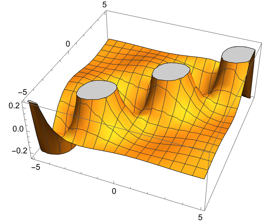
(a) $a=b=1$

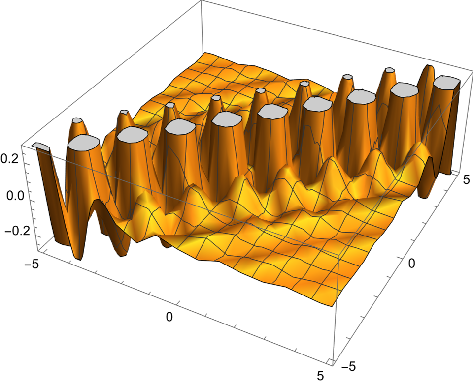
(b) $a=b=3$

Figure 1: Ground truth model for our simulation study, defined in (5).

In this section, we demonstrate through Monte Carlo simulations that our non-parametric bootstrap method outperforms the naive theoretical confidence intervals from classical regression analysis. Specifically, we show that our approach attains a more favorable Pareto frontier representing the trade-off between interval width and coverage probability.

4.1 Naive Confidence Intervals

To obtain confidence intervals for our explanations, one could naively assume that the sampling distribution of the estimated feature importance score is asymptotically a Gaussian distribution centered around the true importance score. This is true if one is estimating partial derivatives using local polynomial regression and if the following assumptions from classical regression analysis hold: (i) The model is well-specified (it locally matches the true underlying model). (ii) Any error in the fit is due to mean-zero, i.i.d. Gaussian noise. In this case, the confidence interval of the importance score at confidence level $100\times(1-\alpha)\%$ is given by the closed-form expression

$$\Big{[}\hat{\theta}-z^{*}\cdot\text{se}(\hat{\theta}),\quad\hat{\theta}+z^{*}\cdot\text{se}(\hat{\theta})\Big{]}.$$ (1)

Here, $\hat{\theta}$ is the point estimator of the partial derivative, $z^{*}$ is the z-score corresponding to confidence level $100\times(1-\alpha)\%$, and $\text{se}(\hat{\theta})$ is the standard error of the sampling distribution. For example, if a $95\%$ confidence level is desired, the resulting bounds are $\hat{\theta}\pm 1.96\times\text{se}(\hat{\theta})$.

Since the local polynomial model is linear in the regression coefficients, it follows that the partial derivative of the model with respect to any feature is also linear in the coefficients. Hence, $\text{se}(\hat{\theta})\triangleq\sqrt{\text{Var}(\hat{\theta})}$ can be determined by computing the variance of a linear combination of the regression coefficients as follows. For simplicity, we consider the one-dimensional case and note that the derivation extends straightforwardly to the case of multiple covariates. Let $g$ be the local polynomial model used in our explanation, which can be expressed as $g(x)=\sum_{\ell=0}^{k}\hat{\beta}_{\ell}\cdot x^{\ell}$. Then the estimated feature importance score is given by $\hat{\theta}=g^{\prime}(x)=\hat{\beta}^{\top}v$, where $\hat{\beta}=\begin{bmatrix}\hat{\beta}_{1}&\hat{\beta}_{2}&\cdots&\hat{\beta}_{k}\end{bmatrix}^{\top}$ and $v\in\mathbb{R}^{k}$ is a vector with $v_{\ell}=\ell\cdot x^{\ell-1},\,\ell\in\{1,2,\ldots,k\}$. It follows that

$$\text{Var}(\hat{\theta})=\text{Var}(\hat{\beta}^{\top}v)=v^{\top}\Sigma v,$$ (2)

where $\Sigma\in\mathbb{R}^{k\times k}$ is the variance-covariance matrix of regression coefficients, such that $\Sigma_{ij}=\text{Cov}(\hat{\beta}_{i},\hat{\beta}_{j})$ for $i,j\in\{1,\ldots,k\}$. In the case of the least squares estimator, we have

$$\hat{\beta}=(X^{\top}X)^{-1}X^{\top}y,\quad\Sigma=(X^{\top}X)^{-1}\sigma^{2},$$ (3)

where $\sigma^{2}$ (the noise variance) can be estimated as

$$\hat{\sigma}^{2}=\frac{1}{m-d-1}\sum_{z\in\mathcal{N}_{x^{*}}}\Big{(}f(z)-g(z)\Big{)}^{2}.$$ (4)

4.2 Simulation Results

As a ground truth model, we use the function

$$S(x_{1},x_{2},a,b)=\sin(a\cdot x_{1})\cdot\cos(b\cdot x_{2})\cdot\tan\Bigg{(}\frac{1}{1+(x_{1}-x_{2})^{2}}\Bigg{)},$$ (5)

where $x_{1},x_{2}\in[-5,5]$ are continuous features and $a,b\in\{1,2,3\}$ are categorical features. The model is depicted for two different values of $a$ and $b$ in Figure 1. This function captures several complex characteristics often found in real-world ML models: it is not defined everywhere, it approaches infinity in some regions, and it is drastically sensitive to changes in the categorical values.

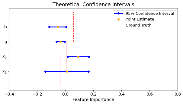
(a)

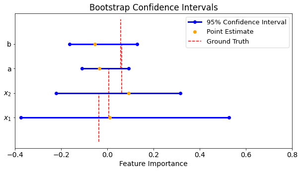
(b)

Figure 2: Simulated comparison between the theoretical and bootstrap intervals with $n=2{,}000$.

As a proof of concept, Figure 2 compares our method to the naive confidence intervals (using a significance level of 5% in both cases) at a randomly selected instance in the simulated data. The plot shows that our bootstrap interval captures the true feature importance scores for all of the features, whereas the naive confidence interval is too narrow for all but one of the features $(x_{1})$. Of course, in this particular example, one could improve the performance of the naive intervals simply by “stretching” them (e.g., using a 99% confidence level to increase their width). Thus, it does not make sense to compare interval widths without controlling for coverage rate, and vice versa.

To ensure a proper comparison between the naive and bootstrap intervals, we analyze each method’s “Pareto frontier” for variable $x_{1}$ of the ground truth model. Specifically, we vary $m$, $m^{\prime}$ and $k$, and for each parameter set, we sample $p$ points from the function (5). Using those $p$ samples, we compute the average interval width and the empirical coverage probability for both the naive confidence interval and our bootstrap uncertainty interval. This yields two sets of tuples—one set corresponding to the naive intervals, the other to the bootstrap—-of the form $(\texttt{Average Interval Width},\,\texttt{Coverage Rate})$. To visualize the Pareto frontier, we plot these points in the two-dimensional plane as shown in Figure 3(a).

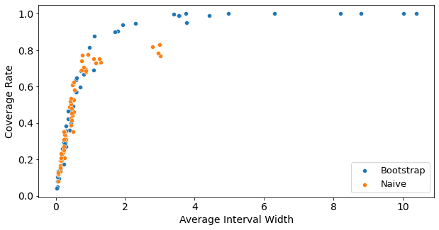
(a) Naive confidence intervals

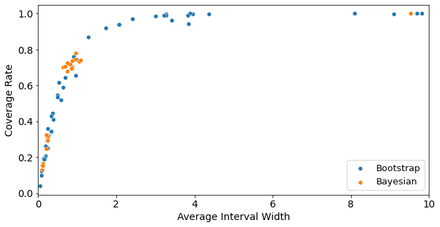
(b) BayesLIME

Figure 3: Comparison of the Pareto frontiers of the bootstrap uncertainty intervals and other methods.

Figure 3(a) shows that our bootstrap method weakly dominates the naive theoretical intervals. For low coverage rates, the naive intervals and the bootstrap intervals exhibit the same trade-off between coverage rate and average interval width. However, around a coverage rate of $0.8$, the naive intervals begin expanding with little gain in coverage rate, whereas the bootstrap method continues to increase its coverage rate as the interval widens. The intuition behind this result is two-fold. First, our bootstrap intervals are not centered around the point estimate, which allows them to have a higher coverage rate for a given interval width. Second, both methods have higher coverage rates when the local neighborhood is of moderate size but the polynomial degree is relatively high. This means that the naive approach has very few degrees of freedom, resulting in intervals that are not wide enough to cover the true parameter unless the point estimate is sufficiently close to the ground truth.

4.3 Choosing Hyperparameters

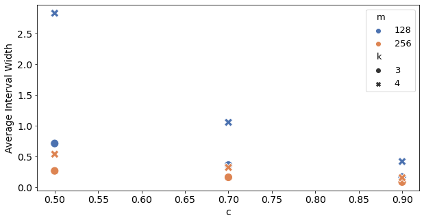
Figure 4: Average width of bootstrap uncertainty intervals as a function of $m,k,c$.

Figure 3(a) also provides important guidance on how to choose hyperparameters. Since, in general, the points lie on the Pareto frontier (aberrations are likely due to noise in the Monte Carlo procedure), a practitioner can specify a desired average interval width and set the hyperparameters to meet such a specification. While it would be impossible to know the coverage rate without a ground truth, the fact that all points lie on the Pareto frontier guarantee that no choice of hyperparameters is inefficient. That is, for a given choice of hyperparameters yielding a particular average interval width, there is not another set of hyperparameters yielding the same interval width with a higher coverage rate.

Figure 4 shows how to adjust the hyperparameters to achieve a desired interval width. Generally speaking, increasing $m^{\prime}$ decreases the interval width, as illustrated by the downward tendency of the points. Increasing $m$ also decreases the interval width, as illustrated by the higher positioning of the blue points compared to the orange points. Finally, increasing $k$ increases the interval width, as illustrated by the higher positioning of the x marks compared to the o marks. These patterns make intuitive sense: the larger the fraction of points $c$ used to compute the intervals, the larger the “overlap” between the bootstrap samples, and thus the smaller the resulting interval width. The larger the local neighborhood ($m$), the less likely it is that the polynomial model captures the true ML model over the entire region; and if the true model varies significantly more than the flexibility of the polynomial allows, the polynomial coefficients will attenuate toward $0$ and the resulting bootstrap interval width will decrease. Finally, higher-degree polynomials exhibit higher variance and have fewer degrees of freedom; thus, the bootstrap distribution is wider for larger $k$.

4.4 Comparison with BayesLIME

BayesLIME [35] is an existing method for quantifying the uncertainty of model-agnostic explanations. In this section, we compare our bootstrap-based explanations and uncertainty measures with those of BayesLIME. We emphasize, however, that the environment for which BayesLIME was developed is different from ours in that BayesLIME assumes access to the underlying machine learning model and the ability to take an arbitrarily large number of samples from it. This inhibits a perfect apples-to-apples comparison between our bootstrap method and BayesLIME. However, we take the following measures to increase the fairness of the comparison: (i) We adapt BayesLIME to only leverage samples from the same fixed dataset available to our bootstrap method. (ii) To ensure that BayesLIME is not handicapped by its assumption of linearity, we endow BayesLIME with the ability to fit higher-order polynomials. The purpose of this exercise is not to show that our bootstrap method is unambiguously better than BayesLIME, but instead to show that when the assumption of model access is loosened, the leading methods that rely on model access may no longer be appropriate.

Figure 3(b) once again plots the Pareto frontier representing the trade-off between interval width and coverage rate. As in the case of the naive uncertainty intervals (Figure 3(a)), BayesLIME does not acheive a coverage rate above $0.8$—unless the intervals are made impractically large. While there may be intermediate parameter sets in which BayesLIME achieves a coverage rate greater than $0.8$, its greater sensitivity to hyperparameter selection inhibits its practicality. On the other hand, our bootstrap method traces a relatively smooth curve through the space and enables practitioners to better fine-tune their desired interval width. This provides evidence that without model access, our bootstrap method can achieve higher coverage rates than BayesLIME with more flexibility in setting the hyperparameters.

5 Experiments with Real-World Data and Models

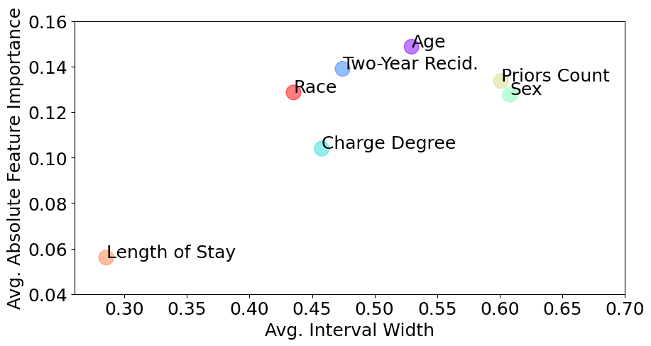
(a) COMPAS + random forest

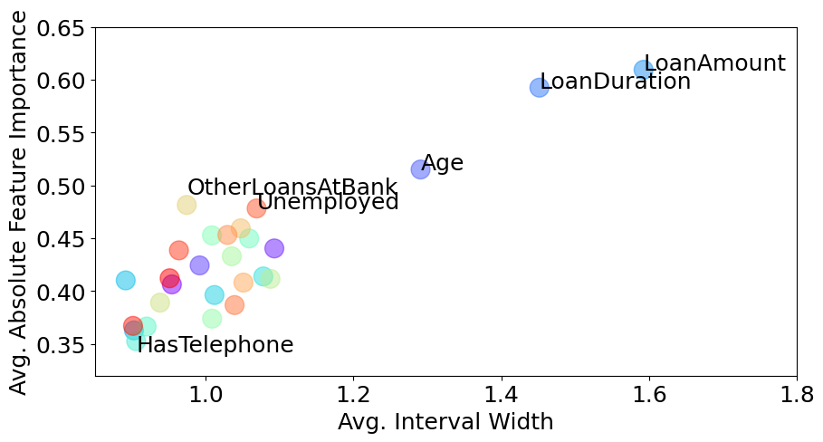
(b) German Credit + random forest

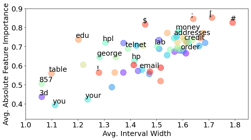
(c) Spambase + SAINT neural network

Figure 5: Visual summary of feature importance scores and corresponding uncertainty measures for models trained on three different datasets.

We further demonstrate the capabilities of our method by applying it to models trained on three well-known tabular datasets: the German Credit and Spambase datasets from the UCI machine learning repository [12], and the COMPAS recidivism dataset [6].

5.1 Random Forest Classifiers

For the German Credit and COMPAS datasets, we trained a random forest classifier with $100$ estimators on a random 80-20 train-test split. We treated the resulting classifier as a black-box model and collected its predictions on the entire dataset to form our static dataset of model inputs and outputs. Due to the step-function-like behavior of the random forest models, we estimated the function differences with our bootstrap method instead of the partial derivatives. Additionally, before performing local regression, we standardized the continuous features, one-hot encoded the categorical features, and transformed the response (i.e., the probabilities predicted by the model) to log-odds. (However, we converted log-odds back to probabilities when estimating the feature importance scores and uncertainty intervals.) The parameters we used were $k=2,\,m=40,\,c=0.9$ and $k=2,\,m=150,\,c=0.667$ for the German Credit and COMPAS datasets, respectively.

We generated an explanation of model behavior for every instance in the test set and computed the following quantities for each feature: (i) the average absolute feature importance score (i.e., the magnitude of the estimated importance assigned to each feature, averaged over all test instances); and (ii) the average width of the uncertainty intervals. Figure 5 plots the resulting $(\texttt{width},\,\texttt{importance})$ tuples for each feature. These plots provide a high-level view of the average influence of each feature on the model’s predictions, along with the corresponding uncertainty that arises from using a finite sample to estimate these quantities. For example, Figure 5(a) shows that the Priors Count and Sex features have a high average importance but are also accompanied by high uncertainty. On the other hand, Length of Stay has a lower average importance but also lower uncertainty. Finally, the Race feature has a relatively high average importance along with a moderate level of uncertainty. Similar observations can be made about Figure 5(b). We see that the OtherLoansAtBank and Unemployed features have both high average importance and low uncertainty, whereas LoanDuration and LoanAmount have higher uncertainty, and HasTelephone has both low average importance and low uncertainty. In practice, after making such observations, one might further investigate the model for issues related to bias and fairness, or attempt to improve the fidelity of the explanation by collecting more data based on the highest-uncertainty features.

5.2 Deep Neural Network

To demonstrate the utility of our method for more complex models, we used SAINT [37], which is an attention-based neural network for tabular data recently shown to outperform more traditional tabular learning algorithms on a variety of supervised and semi-supervised tasks. We trained the model with its default parameters on the Spambase dataset. Each row in the dataset is an email which is labeled as either spam or non-spam. Each email is represented by 57 features, most of which measure the frequencies of different words or characters in the message. As with the random forest classifiers, we treated the SAINT model as a black box and collected its inputs and outputs on the dataset. We also estimated the function differences of the model with respect to each feature, and we applied the same standardization and encoding procedures specified in Section 5.1 before performing polynomial regression. The parameters we used were $k=2,\,m=150,\,c=0.9$.

Figure 5(c) plots, for each feature, the absolute feature importance score and bootstrap interval width, averaged over all instances in the validation set. Somewhat unsurprisingly, keywords and characters such as $\texttt{money},\texttt{addresses},\texttt{credit},\texttt{order},\texttt{\$}$, and # had high average absolute importance scores. However, they also had relatively large interval widths. One possible explanation is that these words and characters commonly appear in both spam and non-spam emails (e.g., confirmations for online shopping orders). Therefore, it is unclear whether these features are truly as indicative of the spam label as their importance scores would suggest. Examples of high-importance, mid-interval-width features include $\texttt{edu},\texttt{hpl},$ and george, the presence of which likely increase the probability that a message is non-spam. Lastly, features such as you and your had relatively small importance scores and interval widths, matching our intuition that such commonly used words would not be particularly influential features in a spam classifier.

6 Conclusions and Open Problems

We proposed a method for generating local explanations from a fixed dataset of model queries, obviating the need for direct model access. An essential component of our method is a non-parametric bootstrapping technique for quantifying the uncertainty in the explanations, motivated by the fact that our setting does not fit neatly into the standard statistical estimation paradigm. Through simulation studies, we showed that our bootstrap confidence intervals outperform (i) a theoretical approach from frequentist statistics that makes strong distributional assumptions about the estimated feature importance scores; and (ii) a Bayesian method for quantifying the uncertainty in explanations [35]. Lastly, we applied our method to three real-world datasets and demonstrated its ability to simultaneously yield insights into the behavior of the black-box model as well as the inherent uncertainty of our explanations due to the fixed nature of the query data.

An important use-case we omitted is that of image and language models. In theory, our method can be applied as-is to both types of models: we can fit a local interpretable model, compute derivatives or finite differences, and generate bootstrap uncertainty intervals. However, without the ability to query the model directly, computing a local model is likely infeasible. For example, when applying LIME to image data, the importance of a super-pixel is estimated by “blacking out” a region in the image and comparing the model’s output on the blacked-out image with its output on the original image. To compute the explanations (and thus uncertainty intervals), our method would require a specialized dataset consisting of complete images as well as blacked-out images. An alternative approach would be to “steal” the model by training another model on the given dataset, using the stolen model as a surrogate for the true model, then fitting an interpretable model to the surrogate. However, training the (possibly large and complex) surrogate model may be too computationally intensive to be practical. Furthermore, if the dataset is not sufficiently dense around the input point of interest, the output of the surrogate model will not be aligned with the output of the true model. For these reasons, building model explanations and uncertainty intervals for language and image models from low-density datasets remains an open problem.

Appendix A Algorithms and Time Complexity

Algorithm 1 Estimating feature importance scores via local polynomial regression

1:  Input: Instance $x^{*}\in\mathbb{R}^{d}$, dataset $\mathcal{D}$, polynomial degree $k$, neighborhood size $m$, proximity function $\pi_{x^{*}}(\cdot)$

2:  Initialize: $Z\in\mathbb{R}^{d}$

3:  $\mathcal{N}_{x^{*}}\leftarrow m$ closest points to $x^{*}$ in $\mathcal{D}$ according to $\pi_{x^{*}}(\cdot)$

4:  $y\leftarrow$ labels of points in $\mathcal{N}_{x^{*}}$, taken from $\mathcal{D}$

5:  $X\leftarrow$ design matrix of points in $\mathcal{N}_{x^{*}}$, transformed to polynomial features of degree $k$ with interaction terms

6:  $\hat{\beta}\leftarrow(X^{\top}X)^{-1}X^{\top}y$

7:  $g\leftarrow$ degree-$k$ polynomial with interaction terms, parameterized by $\hat{\beta}$

8:  for $j=1$ to $d$ do

9:     if feature $j$ is continuous then

10:        $Z_{j}\leftarrow\frac{\partial g}{\partial x_{j}}(x^{*})$ or $g(x^{*}_{+})-g(x^{*}_{-})$

11:     else if feature $j$ is categorical then

12:        $Z_{j}\leftarrow g(x^{*})-g(x^{*}_{\text{base}})$

13:     end if

14:  end for

15:  return $Z$

Algorithm 2 Constructing bootstrap uncertainty intervals

1:  Input: Instance $x^{*}\in\mathbb{R}^{d}$, dataset $\mathcal{D}$, polynomial degree $k$, neighborhood size $m$, number of bootstrap samples $B$, bootstrap neighborhood proportion $c$, significance level $\alpha\in[0,1]$

2:  Initialize: $Z\in\mathbb{R}^{B\times d}$

3:  $\mathcal{N}_{x^{*}}\leftarrow m$ closest points to $x^{*}$ in $\mathcal{D}$ according to $\pi_{x^{*}}(\cdot)$

4:  for $i=1$ to $B$ do

5:     $\mathcal{N}_{x^{*}}^{\prime}\leftarrow\lfloor cm\rfloor$ points sampled uniformly from $\mathcal{N}_{x^{*}}$

6:     $y\leftarrow$ labels of points in $\mathcal{N}_{x^{*}}^{\prime}$, taken from $\mathcal{D}$

7:     $X\leftarrow$ design matrix of points in $\mathcal{N}_{x^{*}}^{\prime}$, transformed to polynomial features of degree $k$ with interaction terms

8:     $\hat{\beta}\leftarrow(X^{\top}X)^{-1}X^{\top}y$

9:     $g\leftarrow$ degree-$k$ polynomial with interaction terms, parameterized by $\hat{\beta}$

10:     for $j=1$ to $d$ do

11:        if feature $j$ is continuous then

12:           $Z_{ij}\leftarrow\frac{\partial g}{\partial x_{j}}(x^{*})$ or $g(x^{*}_{+})-g(x^{*}_{-})$

13:        else if feature $j$ is categorical then

14:           $Z_{ij}\leftarrow g(x^{*})-g(x^{*}_{\text{base}})$

15:        end if

16:     end for

17:  end for

18:  for $j=1$ to $d$ do

19:     $L_{j}\leftarrow(100\cdot\frac{\alpha}{2})^{\text{th}}$ percentile of $Z_{:,j}$

20:     $U_{j}\leftarrow(100\cdot(1-\frac{\alpha}{2}))^{\text{th}}$ percentile of $Z_{:,j}$

21:  end for

22:  return $[L_{j},\,U_{j}]$ for each $j\in[d]$

Time Complexity

The complexity of constructing the explanation itself (Algorithm 1) is $O(dn+n\log n+mq^{2}+q^{3})$ using un-weighted regression, where $q$ is the number of covariates used to fit the polynomial model $g$ (which depends on its degree $k$, whether interaction terms are included, how the categorical features are encoded, etc.). The $dn+n\log n$ term is due to the computations for $\mathcal{N}_{x^{*}}$, assuming that sorting takes $O(n\log n)$ time and that $\pi_{x^{*}}(\cdot)$ can be computed in $O(d)$ time. Fitting the local polynomial requires $O(mq^{2}+q^{3})$ time, which can be straightforwardly obtained using the well-known facts that (i) the complexity of a standard matrix product $AB$, where $A\in\mathbb{R}^{a\times b},B\in\mathbb{R}^{b\times c}$, is $O(abc)$; and (ii) the complexity of matrix inversion $A^{-1}$, where $A\in\mathbb{R}^{a\times a}$, is $O(a^{3})$. If weighted regression is used, the resulting complexity is $O(dn+n\log n+m^{2}q+mq^{2}+q^{3})$. The complexities of the non-weighted and weighted versions of our bootstrap algorithm (Algorithm 2) can be determined in a similar manner and are given by $O(dn+n\log n+B(m^{\prime}q^{2}+q^{3}))$ and $O(dn+n\log n+B(m^{\prime 2}q+m^{\prime}q^{2}+q^{3}))$, respectively.

Appendix B Additional Experimental Details

Compute Resources

The experiments were run on an Apple M1 machine with 16 GB of RAM and the macOS Monterey operating system.

Proximity Function

We used the following procedure to select a neighborhood of $m$ points around the input instance $x^{*}$. First, we sort the points in the dataset by the Euclidean distance between their continuous features and those of $x^{*}$. Within this ordering, we then select the first $m$ points that provide an equal representation of the baseline class and the query class for each categorical feature. We enforce this balanced representation to ensure that for each categorical feature, the function difference with respect to the baseline class can be estimated accurately. Further implementation details can be found in the supplemental code.

Weighted Regression

In the experiments where we perform weighted local regression, the weight assigned to the $i^{\text{th}}$ sample in the dataset is given by

$$w_{i}=\frac{1-(\phi_{i}-\min(\phi))}{\max(\phi)-\min(\phi)},$$

where $\phi\in\mathbb{R}^{n}$ is the vector of proximity values between the input instance $x^{*}$ and all other points in the dataset: $\phi_{i}=\pi_{x^{*}}(x^{(i)})$.

Experiment and Figure Parameters

Below we specify the parameters and other settings used to generate Figures 2 through 4:

• Figures 2(a) and 2(b) were generated using a synthetic dataset of size $n=2{,}000$ sampled uniformly from the domain. To construct the explanations, we standardized the continuous features and one-hot encoded the categorical features, then fit a polynomial of degree $k=4$ using weighted least squares regression with the $m=66$ closest points. For the confidence intervals, we drew $B=500$ bootstrap samples of size $m^{\prime}=59$, sampled uniformly from the neighborhood of $m=66$ points.

• Figure 3(a) was generated by sweeping over all combinations of $k\in\{1,2,3,4\}$, $m\in\{32,64,128,256\}$, and setting $m^{\prime}$ such that $m^{\prime}=\lfloor{cm}\rfloor$ with $c\in\{.3,.5,.7,.9\}$. Throughout, $n=2{,}000$ and $p=250$, but qualitatively similar results held for $n\in\{1000,2000,3000,4000,5000\}$.

• Figure 4 was generated by setting $n=2{,}000$ and $p=250$, but qualitatively similar results held for $n\in\{1000,2000,3000,4000,5000\}$.

• Figure 3(b) was generated by sweeping over all combinations of $k\in\{2,3,4\}$, $m\in\{64,128,256\}$, and setting $m^{\prime}$ such that $m^{\prime}=\lfloor{cm}\rfloor$ with $c\in\{.3,.5,.7,.9\}$. Throughout, $n=2{,}000$ and $p=250$, but qualitatively similar results held for $n\in\{1000,2000,4000,5000\}$.

References

- Adadi and Berrada, [2018] Adadi, A. and Berrada, M. (2018). Peeking inside the black-box: a survey on explainable artificial intelligence (XAI). IEEE Access, 6:52138–52160.
- [2] Agarwal, C., Johnson, N., Pawelczyk, M., Krishna, S., Saxena, E., Zitnik, M., and Lakkaraju, H. (2022a). Rethinking stability for attribution-based explanations. arXiv preprint arXiv:2203.06877.
- [3] Agarwal, C., Zitnik, M., and Lakkaraju, H. (2022b). Probing GNN explainers: A rigorous theoretical and empirical analysis of GNN explanation methods. In International Conference on Artificial Intelligence and Statistics, pages 8969–8996. PMLR.
- Alvarez-Melis and Jaakkola, [2018] Alvarez-Melis, D. and Jaakkola, T. S. (2018). On the robustness of interpretability methods. arXiv preprint arXiv:1806.08049.
- Ancona et al., [2019] Ancona, M., Ceolini, E., Öztireli, C., and Gross, M. (2019). Gradient-based attribution methods. In Explainable AI: Interpreting, Explaining and Visualizing Deep Learning, pages 169–191. Springer.
- Angwin et al., [2016] Angwin, J., Larson, J., Mattu, S., and Kirchner, L. (2016). Machine bias. In Ethics of Data and Analytics, pages 254–264. Auerbach Publications.
- Baehrens et al., [2010] Baehrens, D., Schroeter, T., Harmeling, S., Kawanabe, M., Hansen, K., and Müller, K.-R. (2010). How to explain individual classification decisions. The Journal of Machine Learning Research, 11:1803–1831.
- Bartlett and Hughes, [2020] Bartlett, J. W. and Hughes, R. A. (2020). Bootstrap inference for multiple imputation under uncongeniality and misspecification. Statistical Methods in Medical Research, 29(12):3533–3546.
- Bracke et al., [2019] Bracke, P., Datta, A., Jung, C., and Sen, S. (2019). Machine learning explainability in finance: an application to default risk analysis.
- Bykov et al., [2020] Bykov, K., Höhne, M. M.-C., Müller, K.-R., Nakajima, S., and Kloft, M. (2020). How much can I trust you?–quantifying uncertainties in explaining neural networks. arXiv preprint arXiv:2006.09000.
- Došilović et al., [2018] Došilović, F. K., Brčić, M., and Hlupić, N. (2018). Explainable artificial intelligence: A survey. In 2018 41st International Convention on Information and Communication Technology, Electronics and Microelectronics (MIPRO), pages 0210–0215. IEEE.
- Dua et al., [2017] Dua, D., Graff, C., et al. (2017). UCI machine learning repository.
- Efron, [1992] Efron, B. (1992). Bootstrap methods: Another look at the jackknife. In Breakthroughs in Statistics, pages 569–593. Springer.
- Efron and Tibshirani, [1994] Efron, B. and Tibshirani, R. J. (1994). An Introduction to the Bootstrap. CRC press.
- Gilpin et al., [2021] Gilpin, L. H., Penubarthi, V., and Kagal, L. (2021). Explaining multimodal errors in autonomous vehicles. In 2021 IEEE 8th International Conference on Data Science and Advanced Analytics (DSAA), pages 1–10.
- Goodman and Flaxman, [2017] Goodman, B. and Flaxman, S. (2017). European union regulations on algorithmic decision-making and a “right to explanation”. AI Magazine, 38(3):50–57.
- Gulum et al., [2021] Gulum, M. A., Trombley, C. M., and Kantardzic, M. (2021). A review of explainable deep learning cancer detection models in medical imaging. Applied Sciences, 11(10):4573.
- Hama et al., [2022] Hama, N., Mase, M., and Owen, A. B. (2022). Model free variable importance for high dimensional data. arXiv preprint arXiv:2211.08414.
- Hooker et al., [2019] Hooker, S., Erhan, D., Kindermans, P.-J., and Kim, B. (2019). A benchmark for interpretability methods in deep neural networks. Advances in Neural Information Processing Systems, 32.
- Iadarola et al., [2021] Iadarola, G., Martinelli, F., Mercaldo, F., and Santone, A. (2021). Towards an interpretable deep learning model for mobile malware detection and family identification. Computers & Security, 105:102198.
- Kim and Shin, [2021] Kim, D.-s. and Shin, S. (2021). The economic explainability of machine learning and standard econometric models-an application to the US mortgage default risk. International Journal of Strategic Property Management, 25(5):396–412.
- Linardatos et al., [2020] Linardatos, P., Papastefanopoulos, V., and Kotsiantis, S. (2020). Explainable AI: A review of machine learning interpretability methods. Entropy, 23(1):18.
- Litière et al., [2007] Litière, S., Alonso, A., and Molenberghs, G. (2007). Type I and type II error under random-effects misspecification in generalized linear mixed models. Biometrics, 63(4):1038–1044.
- Lundberg and Lee, [2017] Lundberg, S. M. and Lee, S.-I. (2017). A unified approach to interpreting model predictions. Advances in Neural Information Processing Systems, 30.
- Mase et al., [2021] Mase, M., Owen, A. B., and Seiler, B. B. (2021). Cohort shapley value for algorithmic fairness. arXiv preprint arXiv:2105.07168.
- Mohseni et al., [2021] Mohseni, S., Zarei, N., and Ragan, E. D. (2021). A multidisciplinary survey and framework for design and evaluation of explainable AI systems. ACM Transactions on Interactive Intelligent Systems (TiiS), 11(3-4):1–45.
- Nori et al., [2019] Nori, H., Jenkins, S., Koch, P., and Caruana, R. (2019). InterpretML: A unified framework for machine learning interpretability. arXiv preprint arXiv:1909.09223.
- Patro et al., [2019] Patro, B. N., Lunayach, M., Patel, S., and Namboodiri, V. P. (2019). U-cam: Visual explanation using uncertainty based class activation maps. In Proceedings of the IEEE/CVF International Conference on Computer Vision, pages 7444–7453.
- Ribeiro et al., [2016] Ribeiro, M. T., Singh, S., and Guestrin, C. (2016). “Why should I trust you?” Explaining the predictions of any classifier. In Proceedings of the 22nd ACM SIGKDD International Conference on Knowledge Discovery and Data Mining, pages 1135–1144.
- Riedl, [2019] Riedl, M. O. (2019). Human-centered artificial intelligence and machine learning. Human Behavior and Emerging Technologies, 1(1):33–36.
- Schulz et al., [2021] Schulz, J., Poyiadzi, R., and Santos-Rodriguez, R. (2021). Uncertainty quantification of surrogate explanations: an ordinal consensus approach. arXiv preprint arXiv:2111.09121.
- Schwab and Karlen, [2019] Schwab, P. and Karlen, W. (2019). CXPlain: Causal explanations for model interpretation under uncertainty. Advances in Neural Information Processing Systems, 32.
- Silver and Huffman, [2021] Silver, J. and Huffman, T. (2021). Baseball predictions and strategies using explainable AI. In The 15th Annual MIT Sloan Sports Analytics Conference.
- Simonyan et al., [2013] Simonyan, K., Vedaldi, A., and Zisserman, A. (2013). Deep inside convolutional networks: Visualising image classification models and saliency maps. arXiv preprint arXiv:1312.6034.
- Slack et al., [2021] Slack, D., Hilgard, A., Singh, S., and Lakkaraju, H. (2021). Reliable post hoc explanations: Modeling uncertainty in explainability. Advances in Neural Information Processing Systems, 34:9391–9404.
- Smilkov et al., [2017] Smilkov, D., Thorat, N., Kim, B., Viégas, F., and Wattenberg, M. (2017). Smoothgrad: removing noise by adding noise. arXiv preprint arXiv:1706.03825.
- Somepalli et al., [2021] Somepalli, G., Goldblum, M., Schwarzschild, A., Bruss, C. B., and Goldstein, T. (2021). SAINT: Improved neural networks for tabular data via row attention and contrastive pre-training. arXiv preprint arXiv:2106.01342.
- Springenberg et al., [2014] Springenberg, J. T., Dosovitskiy, A., Brox, T., and Riedmiller, M. (2014). Striving for simplicity: The all convolutional net. arXiv preprint arXiv:1412.6806.
- The White House Office of Science and Technology Policy, [2022] The White House Office of Science and Technology Policy (2022). Blueprint for an AI bill of rights. Accessed: 2022-10-24.
- Vansteelandt et al., [2012] Vansteelandt, S., Bekaert, M., and Claeskens, G. (2012). On model selection and model misspecification in causal inference. Statistical Methods in Medical Research, 21(1):7–30.
- Wickstrøm et al., [2020] Wickstrøm, K., Mikalsen, K. Ø., Kampffmeyer, M., Revhaug, A., and Jenssen, R. (2020). Uncertainty-aware deep ensembles for reliable and explainable predictions of clinical time series. IEEE Journal of Biomedical and Health Informatics, 25(7):2435–2444.
- Wilson et al., [2019] Wilson, B., Hoffman, J., and Morgenstern, J. (2019). Predictive inequity in object detection. arXiv preprint arXiv:1902.11097.
- Xu et al., [2019] Xu, F., Uszkoreit, H., Du, Y., Fan, W., Zhao, D., and Zhu, J. (2019). Explainable AI: A brief survey on history, research areas, approaches and challenges. In CCF International Conference on Natural Language Processing and Chinese Computing, pages 563–574. Springer.